Determination of the pole position of the lightest hybrid meson candidate

Abstract

Mapping states with explicit gluonic degrees of freedom in the light sector is a challenge, and has led to controversies in the past. In particular, the experiments have reported two different hybrid candidates with spin-exotic signature, $\pi_{1}(1400)$ and $\pi_{1}(1600)$, which couple separately to $\eta\pi$ and $\eta^{\prime}\pi$. This picture is not compatible with recent Lattice QCD estimates for hybrid states, nor with most phenomenological models. We consider the recent partial wave analysis of the $\eta^{(\prime)}\pi$ system by the COMPASS collaboration. We fit the extracted intensities and phases with a coupled-channel amplitude that enforces the unitarity and analyticity of the $S$-matrix. We provide a robust extraction of a single exotic $\pi_{1}$ resonant pole, with mass and width $1564\pm 24\pm 86{\mathrm{\,Me\kern-1.00006ptV}}$ and $492\pm 54\pm 102{\mathrm{\,Me\kern-1.00006ptV}}$, which couples to both $\eta^{(\prime)}\pi$ channels. We find no evidence for a second exotic state. We also provide the resonance parameters of the $a_{2}(1320)$ and $a^{\prime}_{2}(1700)$.

Introduction.— Explaining the structure of hadrons in terms of quarks and gluons, the fundamental building blocks of Quantum Chromodynamics (QCD), is of key importance to our understanding of strong interactions. The vast majority of observed mesons can be classified as $q\bar{q}$ bound states, although QCD should have, in principle, a much richer spectrum. Indeed, several experiments have reported resonance candidates that do not fit the valence quark model template Ketzer (2012); Meyer and Swanson (2015), mainly in the heavy sector Esposito et al. (2016); Lebed et al. (2017); Guo et al. (2018); Olsen et al. (2018); Karliner et al. (2018). These new experimental results, together with rapid advances in lattice gauge computations, open new fronts in studies of the fundamental aspects of QCD, such as quark confinement and mass generation. Since gluons are the mediators of the strong interaction, QCD dynamics cannot be fully understood without addressing the role of gluons in binding hadrons. The existence of states with explicit excitations of the gluon field, commonly referred to as hybrids, was postulated a long time ago Horn and Mandula (1978); Isgur and Paton (1985); Chanowitz and Sharpe (1983); Barnes et al. (1983); Close and Page (1995), and has recently been supported by lattice Lacock et al. (1997); Bernard et al. (1997); Dudek et al. (2013) and phenomenological QCD studies Szczepaniak and Swanson (2002); Szczepaniak and Krupinski (2006); Guo et al. (2008); Bass and Moskal (2018). In particular, a state with exotic quantum numbers $J^{PC}(I^{G})=1^{-+}(1^{-})$ in the mass range $1.7-1.9{\mathrm{\,Ge\kern-1.00006ptV}}$ is generally expected. The experimental determination of hybrid hadron properties —e.g. their masses, widths, and decay patterns— provides a unique opportunity for a systematic study of low-energy gluon dynamics. This has motivated the COMPASS spectroscopy program Baum et al. (1996); Abbon et al. (2015) and the 12${\mathrm{\,Ge\kern-1.00006ptV}}$ upgrade of Jefferson Lab, with experiments dedicated to hybrid photoproduction at CLAS12 and GlueX Rizzo (2016); Dobbs (2018).

The hunt for hybrid mesons is challenging, since the spectrum of particles produced in high energy collisions is dominated by nonexotic resonances. The extraction of exotic signatures requires sophisticated partial-wave amplitude analyses. In the past, inadequate model assumptions and limited statistics resulted in debatable results. The first reported hybrid candidate was the $\pi_{1}(1400)$ in the $\eta\pi$ final state Thompson et al. (1997); Chung et al. (1999); Adams et al. (2007); Abele et al. (1998, 1999). Another state, the $\pi_{1}(1600)$, was later claimed in the $\rho\pi$ and $\eta^{\prime}\pi$ channels, with different resonance parameters Ivanov et al. (2001); Khokhlov (2000). The COMPASS experiment confirmed a peak in $\rho\pi$ and $\eta^{\prime}\pi$ at around $1.6{\mathrm{\,Ge\kern-1.00006ptV}}$ Alekseev et al. (2010); Akhunzyanov et al. (2018) and an additional structure in $\eta\pi$, at approximately $1.4{\mathrm{\,Ge\kern-1.00006ptV}}$ Adolph et al. (2015). A theoretical approach based on a unitarized $U(1)$-extended chiral Lagrangian predicted a $\pi_{1}$ state with mass of about $1400{\mathrm{\,Me\kern-1.00006ptV}}$ decaying mostly into $\eta^{\prime}\pi$ Bass and Marco (2002). A phenomenological unitary coupled-channel analysis of the $\eta^{(\prime)}\pi$ system from E852 data was instead not conclusive Szczepaniak et al. (2003). While the $\pi_{1}(1600)$ is close to the expectation for a hybrid, the observation of two nearby $1^{-+}$ hybrids below 2${\mathrm{\,Ge\kern-1.00006ptV}}$ is surprising. This makes the microscopic interpretation of the $\pi_{1}(1400)$ problematic. Moreover, in the $SU(3)$ limit, Bose symmetry prevents the decay of a hybrid into $\eta\pi$ Close and Lipkin (1987). A tetraquark interpretation of the lighter state might be viable, and would explain why this state has eluded predictions in constituent gluon models. However, this interpretation would lead to the prediction of unobserved doubly charged and doubly strange mesons Chung et al. (2002), and is unfavored in the diquark-antidiquark model Jaffe and Wilczek (2003); Jaffe (2005). Establishing whether there exists one or two exotic states in this mass region is thus a stringent test for the available phenomenological frameworks in the nonperturbative regime.

In Jackura et al. (2017) we analyzed the spectrum of the $\eta\pi$ $D$-wave extracted from the COMPASS data. In this Letter, we extend the mass dependent study to the exotic $P$-wave, and present results of the first coupled-channel analysis of the $\eta^{(\prime)}\pi$ COMPASS data. We establish that a single exotic $\pi_{1}$ is needed and provide a detailed analysis of its properties. We also determine the resonance parameters of the nonexotic $a_{2}(1320)$ and $a_{2}^{\prime}(1700)$.

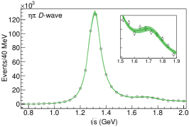
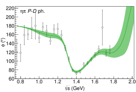
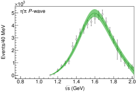
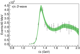
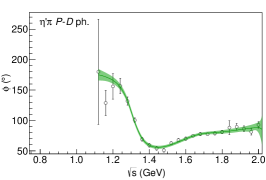
Figure 1: Fits to the $\eta\pi$ (upper line) and $\eta^{\prime}\pi$ (lower line) data from COMPASS Adolph et al. (2015). The intensities of $P$- (left), $D$-wave (center), and their relative phase (right) are shown. The inset zooms into the region of the $a_{2}^{\prime}(1700)$. The solid line and green band show the result of the fit and the $2\sigma$ confidence level provided by the bootstrap analysis, respectively. The initialization of the fit is chosen by randomly generating $O(10^{5})$ different sets of values for the parameters. The best fit has $\chi^{2}/\text{dof}=162/122=1.3$. The errors shown are statistical only.

Description of the data.— We use the mass independent analysis by COMPASS of $\pi p\to\eta^{(\prime)}\pi p$, with a $190{\mathrm{\,Ge\kern-1.00006ptV}}$ pion beam Adolph et al. (2015). We focus on the $P$- and $D$-wave intensities and their relative phase, in both channels. The published data are integrated over the range of transferred momentum squared $-t_{1}\in[0.1,1]{\mathrm{\,Ge\kern-1.00006ptV}}^{2}$. However, given the diffractive nature of the reaction, most of the events are produced in the forward direction, near the lower limit in $-t_{1}$. The $\eta^{(\prime)}\pi$ partial-wave intensities and phase differences are given in 40${\mathrm{\,Me\kern-1.00006ptV}}$ mass bins, from threshold up to 3${\mathrm{\,Ge\kern-1.00006ptV}}$. Intensities are normalized to the number of observed events corrected by the detector acceptance. The errors quoted are statistical only; systematic uncertainties or correlations in the extraction of the partial waves were found to be negligible Schlüter (2012). We thus assume that all data points are independent and normally distributed. As seen in Figs. 4(a) and 5(a) of Adolph et al. (2015), at the $\eta^{\prime}\pi$ mass of $2.04{\mathrm{\,Ge\kern-1.00006ptV}}$ there is a sharp falloff in the $P$-wave intensity, and a sudden change by $50\degree$ in the phase difference between the $P$- and $D$-wave. This behavior might be attributed to another state. The E852 experiment claimed indeed a third exotic $\pi_{1}(2015)$ in the $f_{1}(1285)\pi$ and $\omega\pi\pi$ channels Kuhn et al. (2004); Lu et al. (2005). However, this state is too broad to explain such an abrupt behavior and thus it is difficult to find a compelling explanation. Unfortunately it is not possible to crosscheck this behavior with the $\eta\pi$ relative phase due to lack of data in the $1.8-2.0{\mathrm{\,Ge\kern-1.00006ptV}}$ region. Moreover, fitting these features of the $P$-wave drives the position of the $a_{2}^{\prime}$ to unphysical values. For these reasons, we fit data up to $2{\mathrm{\,Ge\kern-1.00006ptV}}$ only.

Enforcing unitarity allows us to properly implement the interference among the various resonances and the background. In principle, one wishes to include all the kinematically allowed channels in a unitary analysis. Recently, COMPASS published the complete $3\pi$ partial-wave analysis Akhunzyanov et al. (2018), including the exotic $1^{-+}$ wave in the $\rho\pi$ final state. However, the extraction of the resonance pole in this channel is hindered by the irreducible Deck process Deck (1964), which refers to the exchange of a pion between the final state $\rho$ and $\pi$ (cf. Figure 8 in Akhunzyanov et al. (2018)). This generates a peaking background in the exotic partial wave Ascoli et al. (1974); Ryabchikov . Since the Deck mechanism is not fully accounted for in the COMPASS amplitude model, we do not include the $3\pi$ data in our analysis. As discussed in Jackura et al. (2017), neglecting additional channels does not affect the pole position, as long as the resonance poles are far away from threshold, which is the case studied here.

Reaction model.— At high energies, peripheral production of $\pi p\to\eta^{(\prime)}\pi p$ is dominated by Pomeron ($\mathbb{P}$) exchange. The notion of Pomeron exchange emerges from Regge theory Chew and Frautschi (1961); Donnachie et al. (2005), and allows us to factorize the $\pi\mathbb{P}\to\eta^{(\prime)}\pi$ process. For fixed $t_{1}$ the latter resembles an ordinary helicity partial wave amplitude $a^{J}_{i}(s)$, with $i=\eta^{(\prime)}\pi$ the final channel index, $J$ the angular momentum of the $\eta^{(\prime)}\pi$ system and $s$ its invariant mass squared. This amplitude, in principle, also depends on the effective spin and helicity of the Pomeron. However, the approximately constant hadron cross section at high energies implies that the effective spin of the Pomeron is near one, which explains dominance of the partial wave components with angular momentum projection $M=\pm 1$ as seen in data Close and Schuler (1999); Arens et al. (1997); Adolph et al. (2015). Since the two are related by parity, we drop reference to the Pomeron quantum numbers (for more details, see Jackura et al. (2017)). As discussed previously, we fix an effective value $t_{\text{eff}}=-0.1{\mathrm{\,Ge\kern-1.00006ptV}}^{2}$.

We parameterize the amplitudes following the coupled-channel $N/D$ formalism Bjorken (1960),

$$a^{J}_{i}(s)=q^{J-1}p_{i}^{J}\,\sum_{k}n^{J}_{k}(s)\left[{D^{J}(s)}^{-1}\right]_{ki}\,,$$ (1)

where $p_{i}$ is the $\eta^{(\prime)}\pi$ breakup momentum, and $q$ the $\pi$ beam momentum in the $\eta^{(\prime)}\pi$ rest frame. The $n^{J}_{k}(s)$’s incorporate exchange “forces” in the production process and are smooth functions of $s$ in the physical region. The $D^{J}(s)$ matrix represents the $\eta^{(\prime)}\pi\to\eta^{(\prime)}\pi$ final state interactions, and contains cuts on the real axis above thresholds (right hand cuts), which are constrained by unitarity.

For the numerator $n^{J}_{k}(s)$, we use an effective expansion in Chebyshev polynomials. A customary parameterization of the denominator is given by Aitchison (1972)

$$D^{J}_{ki}(s)=\left[{K^{J}(s)}^{-1}\right]_{ki}-\frac{s}{\pi}\int_{s_{k}}^{\infty}ds^{\prime}\frac{\rho N^{J}_{ki}(s^{\prime})}{s^{\prime}(s^{\prime}-s-i\epsilon)},$$ (2)

where $s_{k}$ is the threshold in channel $k$ and

$$\rho N^{J}_{ki}(s^{\prime}) =\delta_{ki}\,\frac{\lambda^{J+1/2}\left(s^{\prime},m_{\eta^{(\prime)}}^{2},m_{\pi}^{2}\right)}{\left(s^{\prime}+s_{L}\right)^{2J+1+\alpha}}$$ (3)

is an effective description of the left hand singularities in the $$\eta^{(\prime)}\pi\to\eta^{(\prime)}\pi s_{L} \simeq 1{\mathrm{\,Ge\kern-1.00006ptV}}^{2}$$ scattering, which is controlled by the parameter fixed at the hadronic scale . Finally,

$$K^{J}_{ki}(s) =\sum_{R}\frac{g^{J,R}_{k}g^{J,R}_{i}}{m_{R}^{2}-s}+c^{J}_{ki}+d^{J}_{ki}\,s,$$ (4)

with $c^{J}_{ki}=c^{J}_{ik}$ and $d^{J}_{ki}=d^{J}_{ik}$, is a standard parameterization for the $K$-matrix. In our reference model, we consider two $K$-matrix poles in the $D$-wave, and one single $K$-matrix pole in the $P$-wave; the numerator of each channel and wave is described by a third-order polynomial. We set $\alpha=2$ in Eq. (3), which has been effective in describing the single-channel case Jackura et al. (2017). The remaining 37 parameters are fitted to data, by performing a $\chi^{2}$ minimization with MINUIT James and Roos (1975). As shown in Fig. 1, the result of the best fit is in good agreement with data. In particular, a single $K$-matrix pole is able to correctly describe the $P$-wave peaks in the two channels, which are separated by $200{\mathrm{\,Me\kern-1.00006ptV}}$. The shift of the peak in the $\eta\pi$ spectrum to lower energies originates from the combination between final state interactions and the production process. The uncertainties on the parameters are estimated via the bootstrap method Press et al. (2007); Efron and Tibshirani (1994): we generate a large number of pseudo datasets and refit each one of them. The (co)variance of the parameters provides an estimate of their statistical uncertainties and correlations. The values of the fitted parameters and their covariance matrix are provided in the Supplemental Material sup . The average curve passes the Gaussian test in Navarro Pérez et al. (2015).

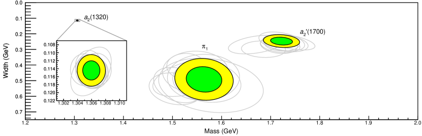
Figure 2: Positions of the poles identified as the $a_{2}(1320)$, $\pi_{1}$, and $a_{2}^{\prime}(1700)$. The inset shows the position of the $a_{2}(1320)$. The green and yellow ellipses show the $1\sigma$ and $2\sigma$ confidence levels, respectively. The gray ellipses in the background show, within $2\sigma$, variation of the pole position upon changing the functional form and the parameters of the model, as discussed in the text

Once the parameters are determined, the amplitudes can be analytically continued to complex values of $s$. The $D^{J}(s)$ matrix in Eq. (2) can be continued underneath the unitarity cut into the closest unphysical Riemann sheet. A pole $s_{P}$ in the amplitude appears when the determinant of $D^{J}(s_{P})$ vanishes. Poles close to the real axis influence the physical region and can be identified as resonances, whereas further singularities are likely to be artifacts of the specific model with no direct physical interpretation. For any practical parameterization, especially in a coupled-channel problem, it is not possible to specify a priori the number of poles. Appearance of spurious poles far from the physical region is thus unavoidable. It is however possible to isolate the physical poles by testing their stability against different parameterizations and data resampling. We select the resonance poles in the $m\in[1,2]{\mathrm{\,Ge\kern-1.00006ptV}}$ and $\Gamma\in[0,1]{\mathrm{\,Ge\kern-1.00006ptV}}$ region, where customarily $m=\operatorname{Re}\sqrt{s_{P}}$ and $\Gamma=-2\operatorname{Im}\sqrt{s_{P}}$. We find two poles in the $D$-wave, identified as the $a_{2}(1320)$ and $a_{2}^{\prime}(1700)$, and a single pole in the $P$-wave, which we call $\pi_{1}$. The pole positions are shown in Fig. 2, and the resonance parameters in Table 1. To estimate the statistical significance of the $\pi_{1}$ pole, we perform fits using a pure background model for the $P$-wave, i.e. setting $g^{P,1}_{\eta^{(\prime)}\pi}=0$ in Eq. (4). The best solution having no poles in our reference region has a $\chi^{2}$ almost 50 times larger, which rejects the possibility for the $P$-wave peaks to be generated by nonresonant production. We also considered solutions having two isolated $P$-wave poles in the reference region, which would correspond to the scenario discussed in the PDG Tanabashi et al. (2018). The $\chi^{2}$ for this case is equivalent to the single pole solution. One of the poles is compatible with the previous determination, while the second is unstable, i.e. it can appear in a large region of the $s$-plane depending on the initial values of the fit parameters. Moreover, the behavior of the $\eta\pi$ phase required by the fit is rather peculiar. A $180^{\circ}$ jump (due to a zero in the amplitude) appears above $1.8{\mathrm{\,Ge\kern-1.00006ptV}}$, where no data exist. We conclude there is no evidence for a second pole.

Systematic uncertainties.— Unlike the COMPASS mass independent fit, the pole extraction carries systematic uncertainties associated with the reaction model. To assess these, we vary the parameters and functional forms which were kept fixed in the previous fits. We can separate these in two categories: $i)$ variations of the numerator function $n^{J}_{k}(s)$ in Eq. (1), which is expected to be smooth in the region of the data, and $ii)$ variations of the function $\rho N(s^{\prime})$, which determines the imaginary part of the denominator in Eq. (2). As for the latter, we investigate whether the specific form we chose biases the determination of the poles. Upon variation of the parameters and of the functional forms, the shape of the dispersive integral in Eq. (2) is altered, but the fit quality is unaffected. The pole positions change roughly within $2\sigma$, as one can see in Fig. 2. As for the numerator $n^{J}_{k}(s)$, we varied the effective value of $t_{\text{eff}}$ and the order of the polynomial expansion. Given the flexibility of the numerator parameterization, these variations effectively absorb the model dependence related to the production mechanism. None of these cause important changes in pole locations. Our final estimate for the uncertainties is reported in Table 1, while the detailed summary is given in the Supplemental Material sup .

Table 1: Resonance parameters. The first error is statistical, the second systematic.

Poles	Mass $(\!{\mathrm{\,Me\kern-1.00006ptV}})$	Width $(\!{\mathrm{\,Me\kern-1.00006ptV}})$
$a_{2}(1320)$	$1306.0\pm 0.8\pm 1.3$	$114.4\pm 1.6\pm 0.0$
$a_{2}^{\prime}(1700)$	$1722\pm 15\pm 67$	$247\pm 17\pm 63$
$\pi_{1}$	$1564\pm 24\pm 86$	$492\pm 54\pm 102$

Conclusions.— We performed the first coupled-channel analysis of the $P$- and $D$-waves in the $\eta^{(\prime)}\pi$ system measured at COMPASS Adolph et al. (2015). We used an amplitude parameterization constrained by unitarity and analyticity. We find two poles in the $D$-wave, which we identify as the $a_{2}(1320)$ and the $a_{2}^{\prime}(1700)$, with resonance parameters consistent with the single-channel analysis Jackura et al. (2017). In the $P$-wave, we find a single exotic $\pi_{1}$ in the region constrained by data. This determination is compatible with the existence of a single isovector hybrid meson with quantum numbers $J^{PC}=1^{-+}$, as suggested by lattice QCD Lacock et al. (1997); Bernard et al. (1997); Dudek et al. (2013). Its mass and width are determined to be $1564\pm 24\pm 86{\mathrm{\,Me\kern-1.00006ptV}}$ and $492\pm 54\pm 102{\mathrm{\,Me\kern-1.00006ptV}}$, respectively. The statistical uncertainties are estimated via the bootstrap technique, while the systematics due to model dependence are assessed by varying parameters and functional forms that are not directly constrained by unitarity. We find no evidence for a second pole that could be identified with another $\pi_{1}$ resonance. Solutions with two poles are possible, but do not improve the fit quality and, when present, the position of the second pole is unstable against different starting values of the fit. It is worth noting that the two-pole solutions have a peculiar behavior of the $\eta\pi$ phase in the $\gtrsim 2{\mathrm{\,Ge\kern-1.00006ptV}}$ mass region, where no data exist. New data from GlueX and CLAS12 experiments at Jefferson Lab in this and higher mass region will be valuable to test this behavior.

I Supplemental material

Table 2: Parameters of the numerator $n^{J}_{k}(s)=\sum_{n=0}^{3}{a^{J,k}_{n}T_{n}\left[\omega(s)\right]}$, with $\omega(s)=s/(s+s_{0})$, and $s_{0}=1{\mathrm{\,Ge\kern-0.90005ptV}}^{2}$ reflects the short range nature of $\eta^{(\prime)}\pi$ production. All numbers are expressed in${\mathrm{\,Ge\kern-0.90005ptV}}$ units. The first values are obtained from the best fit, and should be used to reproduce the plots. The second values contains the mean value and standard deviation estimated with $5\times 10^{4}$ bootstrapped datasets. We remark that the coefficients are $\gtrsim 95\%$ correlated, and the single error has to be taken with care.

$\eta\pi$ channel			$\eta^{\prime}\pi$ channel
$a^{P,\eta\pi}_{0}$	$408.75$	$356\pm 334$	$a^{P,\eta^{\prime}\pi}_{0}$	$-47.05$	$-43\pm 39$
$a^{P,\eta\pi}_{1}$	$-632.57$	$-547\pm 534$	$a^{P,\eta^{\prime}\pi}_{1}$	$65.84$	$59\pm 63$
$a^{P,\eta\pi}_{2}$	$281.48$	$240\pm 255$	$a^{P,\eta^{\prime}\pi}_{2}$	$-20.96$	$-17\pm 30$
$a^{P,\eta\pi}_{3}$	$-57.98$	$-47\pm 63$	$a^{P,\eta^{\prime}\pi}_{3}$	$1.20$	$-0\pm 8$
$a^{D,\eta\pi}_{0}$	$-247.80$	$-247\pm 28$	$a^{D,\eta^{\prime}\pi}_{0}$	$230.92$	$233\pm 79$
$a^{D,\eta\pi}_{1}$	$413.91$	$415\pm 39$	$a^{D,\eta^{\prime}\pi}_{1}$	$-290.66$	$-290\pm 125$
$a^{D,\eta\pi}_{2}$	$-190.94$	$-192\pm 39$	$a^{D,\eta^{\prime}\pi}_{2}$	$176.88$	$177\pm 83$
$a^{D,\eta\pi}_{3}$	$59.25$	$61\pm 29$	$a^{D,\eta^{\prime}\pi}_{3}$	$-3.82$	$-1\pm 62$

Table 3: Parameters of $D^{J}(s)$. The errors and correlations are estimated with bootstrap.

Resonating terms			$K$-matrix background
$g^{P,1}_{\eta\pi}$	$-0.68$	$-0.55\pm 0.38$	$c^{P}_{\eta\pi,\eta\pi}$	$-15.43$	$-14.77\pm 7.22$
$g^{P,1}_{\eta^{\prime}\pi}$	$-13.12$	$-13.12\pm 0.95$	$c^{P}_{\eta\pi,\eta^{\prime}\pi}$	$-67.22$	$-65.28\pm 13.91$
$m^{2}_{P,1}$	$3.52$	$3.52\pm 0.08$	$c^{P}_{\eta^{\prime}\pi,\eta^{\prime}\pi}$	$-190.73$	$-184.19\pm 38.21$
			$d^{P}_{\eta\pi,\eta\pi}$	$1.82$	$1.93\pm 2.24$
			$d^{P}_{\eta\pi,\eta^{\prime}\pi}$	$7.64$	$7.59\pm 5.09$
			$d^{P}_{\eta^{\prime}\pi,\eta^{\prime}\pi}$	$63.85$	$60.54\pm 18.59$
$g^{D,1}_{\eta\pi}$	$5.63$	$5.64\pm 0.34$	$c^{D}_{\eta\pi,\eta\pi}$	$-2402.56$	$-2385.05\pm 273.87$
$g^{D,1}_{\eta^{\prime}\pi}$	$-3.77$	$-3.78\pm 0.10$	$c^{D}_{\eta\pi,\eta^{\prime}\pi}$	$462.60$	$469.55\pm 55.87$
$m^{2}_{D,1}$	$1.86$	$1.86\pm 0.02$	$c^{D}_{\eta^{\prime}\pi,\eta^{\prime}\pi}$	$-86.60$	$-92.25\pm 28.11$
$g^{D,2}_{\eta\pi}$	$147.79$	$147.17\pm 9.88$	$d^{D}_{\eta\pi,\eta\pi}$	$-614.58$	$-608.35\pm 49.32$
$g^{D,2}_{\eta^{\prime}\pi}$	$-33.39$	$-34.07\pm 3.41$	$d^{D}_{\eta\pi,\eta^{\prime}\pi}$	$164.72$	$166.85\pm 17.46$
$m^{2}_{D,2}$	$8.06$	$8.06\pm 0.30$	$d^{D}_{\eta^{\prime}\pi,\eta^{\prime}\pi}$	$-42.19$	$-44.45\pm 11.59$

Table 4: Summary of systematic studies of the denominator. For each systematic variation, $5\times 10^{4}$ bootstrapped pseudodatasets are produced, and the average is shown here. For each parameter varied, we consider the maximum deviation of the pole position from the one in the reference fit. If that is compatible with the statistical uncertainty, we neglect the effect. If larger, we assign a systematic uncertainty to it, and eventually add in quadrature all the systematic uncertainties. We vary the value of $s_{L}$ and $\alpha$ in the reference model in Eq. (2). As an alternative model, we use $\rho N^{J}_{ki}(s^{\prime})=\delta_{ki}\,Q_{J}(z_{s^{\prime}})\,s^{\prime-\alpha}\lambda^{-1/2}(s^{\prime},m^{2}_{\eta^{(\prime)}},m^{2}_{\pi})$, where $Q_{J}(z_{s^{\prime}})$ is the second kind Legendre function, and $z_{s^{\prime}}=1+2s^{\prime}s_{L}/\lambda(s^{\prime},m^{2}_{\eta^{(\prime)}},m^{2}_{\pi})$, with $s_{L}=1{\mathrm{\,Ge\kern-0.90005ptV}}^{2}$. Asymptotically it behaves as $s^{\prime-\alpha}$, has a left hand cut starting at $s^{\prime}=0$, a short cut between $(s^{\prime}-m_{\eta^{(\prime)}})^{2}$ and $(s^{\prime}+m_{\eta^{(\prime)}})^{2}$, and an incomplete circular cut.

Systematic	Poles	Mass $(\!{\mathrm{\,Me\kern-1.00006ptV}})$	Deviation $(\!{\mathrm{\,Me\kern-1.00006ptV}})$	Width $(\!{\mathrm{\,Me\kern-1.00006ptV}})$	Deviation $(\!{\mathrm{\,Me\kern-1.00006ptV}})$
Variation of the function $\rho N(s^{\prime})$
${s}_{{L}}=0.8{\mathrm{\,Ge\kern-1.00006ptV}}^{2}$	$a_{2}(1320)$	$1306.4$	$0.4$	$115.0$	$0.6$
	$a_{2}^{\prime}(1700)$	$1720$	$-3$	$272$	$26$
	$\pi_{1}$	$1532$	$-33$	$484$	$-8$
${s}_{{L}}=1.8{\mathrm{\,Ge\kern-1.00006ptV}}^{2}$	$a_{2}(1320)$	$1305.6$	$-0.4$	$113.2$	$-1.2$
	$a_{2}^{\prime}(1700)$	$1743$	$21$	$254$	$7$
	$\pi_{1}$	$1528$	$-36$	$410$	$-82$
Systematic assigned	$a_{2}(1320)$		$0.0$		$0.0$
	$a_{2}^{\prime}(1700)$		$21$		$26$
	$\pi_{1}$		$36$		$82$
$\alpha=1$	$a_{2}(1320)$	$1305.9$	$-0.1$	$114.7$	$0.3$
	$a_{2}^{\prime}(1700)$	$1685$	$-37$	$299$	$52$
	$\pi_{1}$	$1506$	$-58$	$552$	$60$
Systematic assigned	$a_{2}(1320)$		$0.0$		$0.0$
	$a_{2}^{\prime}(1700)$		$37$		$52$
	$\pi_{1}$		$58$		$60$
${Q}_{{J}},\alpha=1$	$a_{2}(1320)$	$1304.9$	$-1.1$	$114.2$	$-0.2$
	$a_{2}^{\prime}(1700)$	$1670$	$-52$	$269$	$22$
	$\pi_{1}$	$1511$	$-53$	$528$	$36$
${Q}_{{J}},\alpha=1.5$	$a_{2}(1320)$	$1306.0$	$0.1$	$115.0$	$0.6$
	$a_{2}^{\prime}(1700)$	$1717$	$-5$	$272$	$25$
	$\pi_{1}$	$1578$	$14$	$530$	$39$
${Q}_{{J}},\alpha=2$	$a_{2}(1320)$	$1306.2$	$0.2$	$114.7$	$0.3$
	$a_{2}^{\prime}(1700)$	$1723$	$1$	$261$	$15$
	$\pi_{1}$	$1570$	$6$	$508$	$16$
Systematic assigned	$a_{2}(1320)$		$1.1$		$0.0$
	$a_{2}^{\prime}(1700)$		$52$		$25$
	$\pi_{1}$		$53$		$0$
Variation of the numerator function $n(s)$
Polynomial expansion	$a_{2}(1320)$	$1305.9$	$-0.1$	$114.7$	$0.3$
	$a_{2}^{\prime}(1700)$	$1723$	$1$	$249$	$2$
	$\pi_{1}$	$1563$	$-1$	$479$	$-13$
Systematic assigned	$a_{2}(1320)$		$0.0$		$0.0$
	$a_{2}^{\prime}(1700)$		$0$		$0$
	$\pi_{1}$		$0$		$0$
${t}_{\text{eff}}=-0.5{\mathrm{\,Ge\kern-1.00006ptV}}^{2}$	$a_{2}(1320)$	$1306.8$	$0.8$	$114.1$	$-0.3$
	$a_{2}^{\prime}(1700)$	$1730$	$8$	$259$	$13$
	$\pi_{1}$	$1546$	$-18$	$443$	$-49$
Systematic assigned	$a_{2}(1320)$		$0.8$		$0.0$
	$a_{2}^{\prime}(1700)$		$0$		$0$
	$\pi_{1}$		$0$		$0$

Table 5: Summary of systematic studies of the numerator. For each systematic variation, $5\times 10^{4}$ bootstrapped pseudodatasets are produced, and the average is shown here. For each parameter varied, we consider the maximum deviation of the pole position from the one in the reference fit. If that is compatible with the statistical uncertainty, we neglect the effect. If larger, we assign a systematic uncertainty to it, and eventually add in quadrature all the systematic uncertainties. We vary the value of $t_{\text{eff}}$, and increase the order of the polynomial expansion by one unit.

Systematic	Poles	Mass $(\!{\mathrm{\,Me\kern-1.00006ptV}})$	Deviation $(\!{\mathrm{\,Me\kern-1.00006ptV}})$	Width $(\!{\mathrm{\,Me\kern-1.00006ptV}})$	Deviation $(\!{\mathrm{\,Me\kern-1.00006ptV}})$
Variation of the numerator function $n(s)$
Polynomial expansion	$a_{2}(1320)$	$1305.9$	$-0.1$	$114.7$	$0.3$
	$a_{2}^{\prime}(1700)$	$1723$	$1$	$249$	$2$
	$\pi_{1}$	$1563$	$-1$	$479$	$-13$
Systematic assigned	$a_{2}(1320)$		$0.0$		$0.0$
	$a_{2}^{\prime}(1700)$		$0$		$0$
	$\pi_{1}$		$0$		$0$
${t}_{\text{eff}}=-0.5{\mathrm{\,Ge\kern-1.00006ptV}}^{2}$	$a_{2}(1320)$	$1306.8$	$0.8$	$114.1$	$-0.3$
	$a_{2}^{\prime}(1700)$	$1730$	$8$	$259$	$13$
	$\pi_{1}$	$1546$	$-18$	$443$	$-49$
Systematic assigned	$a_{2}(1320)$		$0.8$		$0.0$
	$a_{2}^{\prime}(1700)$		$0$		$0$
	$\pi_{1}$		$0$		$0$