Learning One-hidden-layer Neural Networks
under General Input Distributions

Abstract

Significant advances have been made recently on training neural networks, where the main challenge is in solving an optimization problem with abundant critical points. However, existing approaches to address this issue crucially rely on a restrictive assumption: the training data is drawn from a Gaussian distribution. In this paper, we provide a novel unified framework to design loss functions with desirable landscape properties for a wide range of general input distributions. On these loss functions, remarkably, stochastic gradient descent theoretically recovers the true parameters with global initializations and empirically outperforms the existing approaches. Our loss function design bridges the notion of score functions with the topic of neural network optimization. Central to our approach is the task of estimating the score function from samples, which is of basic and independent interest to theoretical statistics. Traditional estimation methods (example: kernel based) fail right at the outset; we bring statistical methods of local likelihood to design a novel estimator of score functions, that provably adapts to the local geometry of the unknown density.

1 Introduction

Neural networks have made significant impacts over the past decade, thanks to their successful applications across multiple domains including computer vision, natural language processing, and robotics. This success partly owes to the mysterious phenomenon that (stochastic) gradient method applied to highly non-convex loss functions converges to a model parameter that achieves high test accuracy. We are in a dire need of theoretical understanding of such phenomenon, in order to guide the design of next generation neural networks and training methods. Significant recent progresses have been made, by asking a simpler question: can we efficiently learn a neural network model, when there is a ground truth neural network that generated the data?

Suppose the data $(x,y)$ is generated by sampling $x$ from an unknown distribution $f_{X}(x)$ and $y$ is generated by passing $x$ through an unknown neural network and adding some simple noise. Even if we train neural networks on this “teacher network”, it is known to be a hard problem without further assumptions (Brutzkus and Globerson,, 2017). Significant effort has been on designing new approaches to learn simple neural networks (such as one-hidden-layer neural network) on data from simple distributions (such as Gaussian) (Tian,, 2017; Ge et al.,, 2017). This is followed by analyses on increasingly more complex architectures (Brutzkus and Globerson,, 2017; Li and Yuan,, 2017). However, the analysis techniques critically depend on the Gaussian input assumption, and further the proposed algorithms are tailored specifically to Gaussian inputs. In this paper, we provide a unified approach to design loss functions that provably learn the true model for a wide range of input distributions with smooth densities.

We consider a scenario where the data is generated from a one-hidden-layer neural network

$$y\;=\;\sum_{i=1}^{k}w_{i}^{\ast}\,g(\langle{a_{i}^{\ast}},{x}\rangle)\,+\,\eta\;.$$ (1)

where the true parameters are $w_{i}^{\ast}\in\mathbb{R}$ and $a_{i}^{\ast}\in\mathbb{R}^{d}$, and $\eta$ is a zero-mean noise independent of $x$, with some non-linear activation function $g:\mathbb{R}\to\mathbb{R}$. It has been widely known that first order methods on the $\ell_{2}$-loss get stuck in bad local minima, even for this simple one-hidden-layer neural networks (Livni et al.,, 2014). If the input $x$ is coming from a Gaussian distribution, Ge et al., (2017) proposes a new loss function $G(\cdot)$ with a carefully designed landscape such that Stochastic Gradient Descent (SGD) provably converges to the true parameters. However, the proposed novel loss function is specifically designed for Gaussian inputs, and gets stuck at bad local minima when applied to general non-Gaussian distributions. We showcase this in Figure 3. Designing the optimization landscape for general input distributions is a practically important and technically challenging problem, as acknowledged in Ge et al., (2017) and many existing works in the literature (Brutzkus and Globerson,, 2017; Tian,, 2017; Li and Yuan,, 2017).

Our goal is to strictly generalize the approach of Ge et al., (2017) and construct a loss function $L(\cdot)$ with a good landscape such that SGD recovers the true parameters with global initializations. The main challenge is in estimating the score function defined as a functional of the probability density function $f(x)$ of the input data $x$:

$$\mathcal{S}_{m}(x)\;\;\triangleq\;\;\frac{\nabla^{(m)}f_{X}(x)}{f_{X}(x)}\;,$$ (2)

where $\nabla^{(m)}f_{X}(x)$ denotes the $m$-th order derivative for an $m\in{\mathbb{Z}}$, which plays a crucial role in the landscape design. We need to evaluate this score function at sample points, which is extremely challenging as it involves the higher order derivatives of a pdf that we do not know. Standard non-parametric density estimation methods such as the Kernel Density Estimators (KDE) (Fukunaga and Hostetler,, 1975) and $k$-Nearest Neighbor methods ($k$NN) all fail to provide a consistent estimator, as they are tailored for density estimation. Existing heuristics do not have even consistency guarantees, which include score matching based methods (Hyvärinen,, 2005; Swersky et al.,, 2011), and de-noising auto-encoder (DAE) based algorithms (Janzamin et al., 2015b, ).

In this paper, we first address this fundamental question of how to estimate the score functions from samples in a principled manner. We introduce a novel approach to adaptively capture the local geometry of the pdf to design a consistent estimator for score functions. To achieve this, we bring ideas from local likelihood methods  (Loader et al.,, 1996; Hjort and Jones,, 1996) from statistics to the context of score function estimation and also prove the convergence rate of our estimator (LLSFE), which is of independent mathematical interest. We further introduce a new loss function for training one-hidden-layer neural networks, that builds upon the estimated score functions. We show that this provably has the desired landscape for general input distributions.

In summary, our main contributions are:

• Score function estimation. In this paper, we provide the first consistent estimator for score functions (and hence the gradients of $L(\cdot)$), which play crucial roles in several recent model parameter learning problems (Hyvärinen,, 2005; Swersky et al.,, 2011; Janzamin et al., 2015b, ). Our provably consistent estimation of score functions, LLSFE, from samples, with local geometry adaptations, is of independent mathematical interest.

• Optimization landscape for general distributions. For a large class of input distributions, with an appropriate score transformation for the input and appropriate tensor projection, we design a loss function $L(\cdot)$ for one-hidden-layer neural network with good landscape properties. In particular, our result is a strict generalization of (Ge et al.,, 2017) which was restricted to Gaussian inputs, in both mathematical and abstract view-points.

Related work. Several recent works have provided provable algorithms for training neural networks (Liang et al.,, 2018; Choromanska et al.,, 2015; Soudry and Hoffer,, 2017; Goel and Klivans,, 2017; Freeman and Bruna,, 2016; Nguyen and Hein,, 2017; Boob and Lan,, 2017). (Arora et al.,, 2014) is an early work on provable learning guarantees on deep generative models for sparse weights. Brutzkus and Globerson, (2017); Tian, (2017) analyze one-hidden-layer neural network with Gaussian input and hidden variables with disjoint supports. (Li and Yuan,, 2017) analyzed the convergence of one-hidden layer neural network with Gaussian input when the true weights are close to identity. (Andoni et al.,, 2014), (Panigrahy et al.,, 2018), (Du and Lee,, 2018) and (Soltanolkotabi et al.,, 2017) studied the optimization landscape of neural networks for some specific activation functions.

Tensor methods have been used to build provable algorithms for training neural networks (Janzamin et al., 2015a, ; Zhong et al.,, 2017). Our work is built upon (Ge et al.,, 2017), which uses a fourth-order tensor based objective function and show good landscape properties. Most of the aforementioned works requires specific assumptions on the input distribution (example: Gaussian), while we only require generic smoothness of the underlying (unknown) density. In a recent work, Ge et al., (2018) provided a learning algorithm using the method of moments for symmetric input distributions. However their techniques are very specific to ReLU activation and do not generalize to general activation functions which we can handle. Zhang et al., (2018) show that gradient descent on empirical loss function based on least squares can recover the true parameters provided the parameters have a good initialization; in contrast, we use global initializations for our algorithm.

Notations. We use $\mathcal{T}(x_{1},\dots,x_{m})$ to denote the inner product for an $m$-th order tensor $\mathcal{T}$ and vectors $x_{1},\dots,x_{m}$. We use $x_{1}\otimes x_{2}\otimes\dots\otimes x_{m}$ to denote outer product of vectors/matrices/tensors. $x^{\otimes j}=x\otimes\dots\otimes x$ denotes the $j$-th order tensor power of $x$ and $x^{\otimes 0}=1$.

$\|\mathcal{T}\|_{{\rm sp}}=\max_{\|u_{i}\|_{2}\leq 1}\mathcal{T}(u_{1},u_{2},\dots,u_{m})$ and $\|\mathcal{T}\|_{\mathcal{F}}=\sqrt{\sum_{i_{1},\dots,i_{m}}(\mathcal{T}_{(i_{1},\dots,i_{m})})^{2}}$ denotes the spectral norm and Frobenius norm of matrix and high-order tensor. ${\rm sym}(\mathcal{T})$ denotes the symmtrify operator of a tensor $\mathcal{T}$ as ${\rm sym}(\mathcal{T})_{(i_{1},\dots,i_{m})}=\frac{1}{m!}\sum_{(j_{1},\dots,j_{m})\in\pi(i_{1},\dots,i_{m})}\mathcal{T}_{(j_{1},\dots,j_{m})}$.

2 Score Function Estimation

In this section, we introduce a new approach for estimating score functions defined in (2) from i.i.d. samples from a distribution. As the score functions involve higher order derivatives of the pdf, it is critical to capture the rate of changes in the pdf. Further, we aim to apply it to data coming from a broad range of distributions. Such sharp estimates for such broad class of distributions can only be achieved by combining the strengths of two popular approaches in density estimation: simple parametric density estimators and complex non-parametric density estimators. We bridge this gap by borrowing the techniques from Local Likelihood Density Estimators (LLDE) and bring them to a new light in order to provide the first consistent score function estimators.

2.1 Local Likelihood Density Estimator (LLDE)

How do we estimate the normalized derivatives of the density? We address this question in a principled manner utilizing the notion local likelihood density estimation (LLDE) from non-parametric methods (Loader et al.,, 1996; Hjort and Jones,, 1996). LLDE is originally designed for estimating density for distributions with complicated local geometry, and can be further applied to estimate functionals of density such as information entropy (Gao et al.,, 2016). Inspired by the fact that LLDEs capture the local geometry of the pdf, we build upon the LLDE estimators to design a new estimator of the higher order derivatives, which is the main bottleneck in score function estimation.

The local likelihood density estimator is specified by a nonnegative function $K:\mathbb{R}^{d}\to\mathbb{R}$ (also called a Kernel function), a degree $p\in\mathbb{Z}^{+}$ of the polynomial approximation, and a bandwidth $h\in\mathbb{R}^{+}$. It is the solution of a maximization of the local log-likelihood function:

$$\mathcal{L}_{x}(f) = \sum_{i=1}^{n}K\Big{(}\frac{X_{i}-x}{h}\Big{)}\log f(X_{i})-n\int K\Big{(}\frac{u-x}{h}\Big{)}f(u)du\;.$$ (3)

For each $x$, we maximize this function over a parametric family of functions $f(\cdot)$, using the following local polynomial approximation of $\log f(x)$:

$$\log f(x) = a_{0}+a_{1}^{T}(u-x)+\frac{1}{2}(u-x)^{T}A_{2}(u-x)+\dots+\frac{1}{p!}\mathcal{A}_{p}(u-x,\dots,u-x)\;,$$ (4)

parameterized by $a=(a_{0},a_{1},A_{2},\dots,\mathcal{A}_{p})\in\mathbb{R}\times\mathbb{R}^{d}\times\mathbb{R}^{d^{2}}\times\dots\times\mathbb{R}^{d^{p}}$. The local likelihood density estimate (LLDE) at point $x$ is defined as $f(x)=e^{\widehat{a}_{0}}$, where $\widehat{a}=(\widehat{a}_{0},\widehat{a}_{1},\widehat{A}_{2},\dots,\widehat{\mathcal{A}}_{p})$ is the maximizer around a point $x$: $\widehat{a}\in\arg\max_{f}{\cal L}_{x}(f)$. The optimization problem can be solved by setting the derivatives $\partial\mathcal{L}_{x}(p)/\partial\mathcal{A}_{j}=0$ for $j\in\{0,\dots,p\}$. The optimal solution $\widehat{a}$ can be obtained from solving the following equations,

$$\int_{\mathbb{R}^{d}}\exp\{a_{0}+a_{1}^{T}(u-x)+\dots+\frac{1}{p!}\mathcal{A}_{p}(u-x)^{\otimes p}\}(\frac{u-x}{h})^{\otimes j}K(\frac{u-x}{h})du\,$$ (5)

$$= \frac{1}{n}\sum_{i=1}^{n}(\frac{X_{i}-x}{h})^{\otimes j}K(\frac{X_{i}-x}{h})\;.$$

We build upon this idea to first introduce the score function estimator, and focus on the statistical aspect of this estimator. We discuss the computational aspect of finding the solution to this optimization in Section 2.4.

2.2 From LLDE to local likelihood score function estimator (LLSFE)

We build upon the techniques from LLDE to design our local likelihood score function estimator (LLSFE). Notice that the score function $\mathcal{S}_{m}(x)$ satisfies the following recursive formula from (Janzamin et al.,, 2014),

$$\mathcal{S}_{m}(x) = -\mathcal{S}_{m-1}(x)\otimes\nabla_{x}\log f(x)-\nabla_{x}\mathcal{S}_{m-1}(x),$$

and $\mathcal{S}_{1}(x)=-\nabla\log f(x)$. This recursion reveals us that the score function can be represented as a polynomial function of the gradients of log-density $(g_{1}(x),G_{2}(x),\dots,\mathcal{G}_{m}(x))=\\ (\nabla\log f(x),\nabla^{(2)}\log f(x),\dots,\nabla^{(m)}\log f(x))$. For example, the polynomial for $\mathcal{S}_{2}(x)$ and $\mathcal{S}_{4}(x)$ are given below:

$$\mathcal{S}_{2}(x) = g_{1}(x)\otimes g_{1}(x)+G_{2}(x)\,$$ (6)

$$\mathcal{S}_{4}(x) = g_{1}(x)\otimes g_{1}(x)\otimes g_{1}(x)\otimes g_{1}(x)+6\,{\rm sym}(G_{2}(x)\otimes g_{1}(x)\otimes g_{1}(x))\,$$ (7)

$$+\,3\,(G_{2}(x)\otimes G_{2}(x))+4\,{\rm sym}(\mathcal{G}_{3}(x)\otimes g_{1}(x))+\mathcal{G}_{4}(x)$$

More generally, the $m$-th order score function can be represented as:

$$\mathcal{S}_{m}(x) = \sum_{\lambda\in\Lambda_{m}}(-1)^{m}c_{m}(\lambda)\,{\rm sym}(\bigotimes_{j\in\lambda}\mathcal{G}_{j})\;,$$ (8)

where $\Lambda_{m}$ denotes the set of partitions of integer $m$ and $c_{m}(\lambda)$ is a positive constant depends on $m$ and the partition, for example, $\Lambda_{4}=\{\{1,1,1,1\},\{2,1,1\},\{2,2\},\{3,1\},\{4\}\}$. Given the polynomial representation of a score function, the LLSFE is given by

$$\widehat{\mathcal{S}^{(p)}_{m}}(x) \triangleq \sum_{\lambda\in\Lambda_{m}}(-1)^{m}c_{m}(\lambda)\,{\rm sym}(\bigotimes_{j\in\lambda}\widehat{\mathcal{A}}_{j}^{(p)})\;.$$ (9)

where $\mathcal{A}_{j}^{(p)}$ is the LLDE estimator of $\mathcal{G}_{j}$ by $p$-degree polynomial approximation.

2.3 Convergence rate of LLSFE

As LLDE captures the local geometry of the pdf, LLSFE inherits this property and is able to consistently estimate the derivatives. This is made precise in the following theorem, where we provide an upper bound of the spectral norm error of the estimated $m$-th order score function. First, we formally state our assumptions.

Assumption 1.

1. The degree of polynomial $p$ is greater than or equal to $m$.

2. The gradient of log-density $\nabla^{(j)}\log f(x)$ at $x$ exists and $\|\nabla^{(j)}\log f(x)\|_{{\rm sp}}\leq C_{j}(x)$ for all $j\in[p+1]$.

3. The non-negative kernel function $K$ satisfies $\int_{\mathbb{R}^{d}}|x_{i}|^{p}K(x)dx<+\infty$ for any $i\in[d]$.

4. Bandwidth $h$ depends on $n$ such that $h\to 0$ and $nh^{d+2m}\to\infty$ as $n\to\infty$.

The following theorem provides an upper bound on the convergence rate of the proposed score function estimator.

Theorem 1.

Under Assumption 1, the spectral norm error of the LLSFE $\widehat{\mathcal{S}^{(p)}_{m}}(x)$ defined in (9) is upper bounded by

$$\|\widehat{\mathcal{S}^{(p)}_{m}}(x)-\mathcal{S}_{m}(x)\|_{\rm sp} \leq O(d^{m/2}h^{p+1-m})+O_{p}(d^{m/2}(nh^{d+2m})^{-1/2}).$$ (10)

Proof.

(Sketch) Note that the estimator is derived by replacing the truth gradients of log-density $(g_{1}(x),G_{2}(x),\dots,\mathcal{G}_{m}(x))$ by the estimates $(\widehat{a}_{0}(x),\widehat{a}_{1}(x),\widehat{A}_{2}(x),\dots,\widehat{\mathcal{A}}_{p}(x))$. Since we assumes that $\|\mathcal{G}_{j}(x)\|_{\rm sp}\leq C_{j}$, so it suffices to upper bound the spectral norm of the error $\|\widehat{\mathcal{A}}_{j}^{(p)}(x)-\mathcal{G}_{j}(x)\|_{\rm sp}$. The following lemma provides upper bounds for each entry of $\widehat{\mathcal{A}}_{j}^{(p)}(x)-\mathcal{G}_{j}(x)$. For simplicity of notation, we fix an $x$ drop the dependency on $x$.

Lemma 2.1.

(Loader et al.,, 1996, Theorem 1) Under Assumption 1 we have

$$\left(\widehat{\mathcal{A}}_{j}^{(p)}\right)_{(i_{1},\dots,i_{j})}-\left(\mathcal{G}_{j}\right)_{(i_{1},\dots,i_{j})} = O(h^{p+1-j})+O_{p}((nh^{d+2j})^{-1/2}),$$ (11)

for any $j\in\{1,\dots,p\}$ and $i_{1},\dots,i_{j}\in[d]^{j}$.

The spectral norm of of the error $\|\widehat{\mathcal{A}}_{j}^{(p)}-\mathcal{G}_{j}\|_{\rm sp}$ is upper bounded by the Frobenius norm. Then applying Lemma 2.1, we have,

$$\|\widehat{\mathcal{A}}_{j}^{(p)}-\mathcal{G}_{j}\|_{\rm sp} \leq O(d^{j/2}h^{p+1-j})+O_{p}(d^{j/2}(nh^{d+2j})^{-1/2}).$$ (12)

Substituting this result into the polynomial representations (8) and (9), we obtain the desired rate. ∎

Remark 1.

By setting $h=n^{-1/(2p+2+d)}$, we obtain

$$\|\widehat{\mathcal{S}^{(p)}_{m}}(x)-\mathcal{S}_{m}(x)\|_{\rm sp} \leq O_{p}(d^{m/2}n^{-(p+1-m)/(2p+2+d)}).$$ (13)

Remark 2.

It was shown in (Stone,, 1980) that the optimal rate for estimating an entry of $\mathcal{G}_{j}$ is $O_{p}(n^{-(p+1-m)/(2p+2+d)})$. We conjecture that LLSFE is also minimax rate-optimal.

2.4 Second Degree LLSFE

In the previous subsection, we proved the convergence rate of the LLSFE. However, the computational cost of LLSFE can be large since numerical integration is needed to compute the integral in (5). To trade off the accuracy and computational cost, we choose Gaussian kernel $K(u)\propto\exp\{\|u\|^{2}/2\}$ and degree $p=2$. This makes the integration in the LHS of (5) tractable and we obtain closed-form expressions for $a_{0}$, $a_{1}$ and $A_{2}$. Using ideas from  (Gao et al.,, 2016, Proposition 1), our estimators for $a_{1}$ and $A_{2}$ are:

$$\widehat{a}_{1} = (\frac{M_{2}}{M_{0}}-(\frac{M_{1}}{M_{0}})(\frac{M_{1}}{M_{0}})^{T})^{-1}\frac{M_{1}}{M_{0}}\;,\,$$ (14)

$$\widehat{A}_{2} = h^{-2}I_{d\times d}-(\frac{M_{2}}{M_{0}}-(\frac{M_{1}}{M_{0}})(\frac{M_{1}}{M_{0}})^{T})^{-1}\;,$$ (15)

where $M_{j}=\sum_{i=1}^{n}(X_{i}-x)^{\otimes j}\exp\{-\frac{\|X_{i}-x\|^{2}}{2h^{2}}\}$ for $j\in\{0,1,2\}$.

The second degree LLSFE is derived by plugging $\widehat{a}_{1}$ and $\widehat{A}_{2}$ into (9). The computational complexity of second degree LLDFE is $O(n\cdot d^{2})$. In the experiments below, we use this second degree estimator and practically show that using second degree estimator as an compromise does not hurt the performance by much.

2.5 Synthetic Simulations of LLSFE

In this experiment we validate the performance of LLSFE, for both Gaussian and non-Gaussian distributions. For Gaussian distribution, we choose $x\sim\mathcal{N}(0,I_{d})$ and $d=2$. The ground truth score functions are $\mathcal{S}_{2}=xx^{T}-I_{d}$ and $\mathcal{S}_{4}=x^{\otimes 4}-6{\rm sym}(x\otimes x\otimes I_{d})+3I_{d}\otimes I_{d}$. We show the spectral error $\|\widehat{\mathcal{S}}_{2}-\mathcal{S}_{2}\|_{\rm sp}$ versus number of sample $n$ for estimation of $\mathcal{S}_{2}$, and the Frobenius error $\|\widehat{\mathcal{S}}_{4}-\mathcal{S}_{4}\|_{\mathcal{F}}$ for estimation of $\mathcal{S}_{4}$ (since computing spectral norm of high-order tensor is NP-hard Hillar and Lim, (2013)). We plot the $\{95\%,75\%,50\%,25\%,5\%\}$ percentiles of our estimation error over $10,000$ independent trials for the estimation of $\mathcal{S}_{2}$ and $50,000$ independent trails for the estimation of $\mathcal{S}_{4}$.

We can see from Figure 1 that all the percentiles of the estimation error decrease as $n$ increases. The log-log scale plot is closed to linear, and the average slope is $-0.5143$ for $\|\widehat{\mathcal{S}}_{2}-\mathcal{S}_{2}\|_{\rm sp}$ and $-0.4984$ for $\|\widehat{\mathcal{S}}_{4}-\mathcal{S}_{4}\|_{\mathcal{F}}$. This suggests that LLSFE is consistent and the error decreases at a faster rate than the theoretical upper bound in Remark 1.

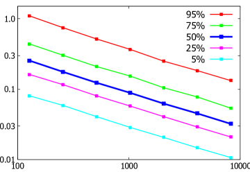
Figure 1: Error of score function estimator versus sample size for $x\sim\mathcal{N}(0,I_{d})$. Top: $\|\widehat{\mathcal{S}}_{2}-\mathcal{S}_{2}\|_{\rm sp}$. Bottom: $\|\widehat{\mathcal{S}}_{4}-\mathcal{S}_{4}\|_{\mathcal{F}}$.

For the non-Gaussian case, we choose $x\sim 0.5\mathcal{N}({\bf 1}_{d},I_{d})+0.5\mathcal{N}(-{\bf 1}_{d},I_{d})$ where ${\bf 1}_{d}$ is the all-1 vector and $d=2$. We also plot the percentiles of the estimation errors in log-log scale in Figure 2. We can see that LLSFE gives a consistent estimate for the non-Gaussian case too, and the rate is $-0.2587$ for $\|\widehat{\mathcal{S}}_{2}-\mathcal{S}_{2}\|_{\rm sp}$ and $-0.1343$ for $\|\widehat{\mathcal{S}}_{4}-\mathcal{S}_{4}\|_{\mathcal{F}}$, which are also faster than the upper bound in Remark 1.

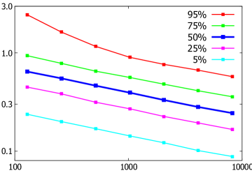
Figure 2: Error of score function estimator versus sample size for $x\sim 0.5\mathcal{N}({\bf\mu},I_{d})+0.5\mathcal{N}(-{\bf\mu},I_{d})$. Top: $\|\widehat{\mathcal{S}}_{2}-\mathcal{S}_{2}\|_{\rm sp}$. Bottom: $\|\widehat{\mathcal{S}}_{4}-\mathcal{S}_{4}\|_{\mathcal{F}}$.

3 Design of landscape

In this section, we show how the proposed density functional estimators can be applied to design a loss function with desired properties, for regression problems under a neural network model. This gives a novel loss function that does not require the data to be distributed as Gaussian, as typically done in existing literature (cf. Section 1 Related work).

Concretely, we consider the problem of training a one-hidden-layer neural network where, for each input $x\in\mathbb{R}^{d}$, the corresponding output is given by

$$\hat{y}(x)\;\;=\;\;\sum_{i=1}^{k}w_{i}\,g(\langle{a_{i}},{x}\rangle)\;,$$ (16)

with weights are $w_{i}\in\mathbb{R}$ and $a_{i}\in\mathbb{R}^{d}$, non-linear activation is $g:\mathbb{R}\to\mathbb{R}$, and the number of hidden neurons is $k\leq d$. Given labeled training data $(x,y)$ coming from some distribution, a standard approach to training such a network is to use the $\ell_{2}$ loss:

$$\ell_{2}(A)\;=\;\mathbb{E}[\|\widehat{y}(x)-y\|^{2}]\;,$$ (17)

as the training objective, where $A$ denotes the weights of the neural network model. However, traditional optimization techniques on $\ell_{2}$ can easily get stuck in local optima as empirically shown in (Livni et al.,, 2014). This phenomenon can be explained precisely under a canonical scenario where the data is generated from a “teacher neural network”:

$$y\;=\;\sum_{i=1}^{k}w_{i}^{\ast}\,g(\langle{a_{i}^{\ast}},{x}\rangle)\,+\,\eta\;.$$ (18)

where the true parameters are $w_{i}^{\ast}\in\mathbb{R}$ and $a_{i}^{\ast}\in\mathbb{R}^{d}$, and $\eta$ is a zero-mean noise independent of $x$. This assumption that the data also comes from a one-hidden-layer neural network is critical in recent mathematical understanding of neural networks, in showing the gain of a shallow ResNet by Li and Yuan, (2017), various properties of the critical points by Tian, (2017), and showing that the standard $\ell_{2}$ minimization is prone to get stuck at non-optimal critical points by Ge et al., (2017). A major limitation of this line of research is that they rely critically on the Gaussian assumption on the data $x$. The analysis techniques use specific properties of spherical Gaussian random variables such that the theoretical findings do not generalize to any other distributions. Further, the estimators designed as per those analyses fail to give consistent estimates for non-Gaussian data.

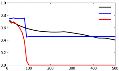
Figure 3: SGD to learn a one-layer-ReLU network in (18) on the proposed objective function $L(A)$ defined in (19) converges to a global minimum with random initialization, whereas on $\ell_{2}$-loss $\ell_{2}(A)$ and $G(A)$, it gets stuck at bad local minima. Left: First 500 iterations. Right: 500-10,000 iterations.

We showcase this limitation in Figure 3, where the data is generated from a Laplacian distribution. The details of this experiment is provided in Section 4.1. Minimizing $\ell_{2}$ loss converges slowly and gets stuck at sub-optimal critical points, consistent with previous observations (Li and Yuan,, 2017). To overcome this weakness Ge et al., (2017) proposed applying Stochastic Gradient Descent (SGD) on a novel loss function $G(A)$ designed from the analysis under the Gaussian assumption. This fails to converge to an optimal critical point for non-Gaussian distributions. To overcome this limitation, we propose a novel loss function $L(A)$ that generalizes to a broad class of distributions.

We focus on the task of recovering the weights $a_{i}^{*}$’s, and denote the set by a matrix $A^{\top}=[a_{1}|\ldots|a_{k}]\in\mathbb{R}^{d\times k}$. The scalar weights $w_{i}^{*}$’s can be separately estimated using standard least squares, once $A$ has been recovered. We propose applying SGD on a new loss function $L(A)$, defined as

$$L(A)\;=\sum_{i,j\in[k],i\neq j}\mathbb{E}[y\cdot t_{1}(x,a_{i},a_{j})]-\mu\sum_{i\in[k]}\mathbb{E}[y\cdot t_{2}(x,a_{i})]+\lambda\sum_{i\in[k]}(\left\|a_{i}\right\|-1)^{2}\;,$$ (19)

where $\mu,\lambda>0$ are regularization coefficients, and

$$t_{1}(x,u,v) = \mathcal{S}_{4}(x)(u,u,v,v),\,$$

$$t_{2}(x,u) = \mathcal{S}_{4}(x)(u,u,u,u),\;u,v\in\mathbb{R}^{d}.$$ (20)

are the applications of the score functions $\mathcal{S}_{m}(x)=\nabla^{(m)}f(x)/f(x)$ on the weight vectors $a_{i}$’s that we are optimizing over, i.e. $\mathcal{S}_{4}(x)(u,v,w,z)=(1/f(x))\sum_{i_{1},i_{2},i_{3},i_{4}}\nabla_{x_{i_{1}}x_{i_{2}}x_{i_{3}}x_{i_{4}}}f(x)u_{i_{1}}v_{i_{2}}w_{i_{3}}z_{i_{4}}$. We provide formulas for some simple distributions below.

Example 1 (Gaussian).

If $x\sim\mathcal{N}(0,I_{d})$, we have that $t_{2}^{(G)}(x,u)=(u^{\top}x)^{4}-6\left\|u\right\|^{2}(u^{\top}x)^{2}+3\left\|u\right\|^{4}$ and $t_{1}^{(G)}(x,u,v)=(u^{\top}x)^{2}(v^{\top}x)^{2}-\left\|u\right\|^{2}(v^{\top}x)^{2}-4(u^{\top}x)(v^{\top}x)(u^{\top}v)-\left\|v\right\|^{2}(u^{\top}x)^{2}+\left\|u\right\|^{2}\left\|v\right\|^{2}+2(u^{\top}v)^{2}$.

Example 2 (Mixture of Gaussians).

If $x\sim p\mathcal{N}(\mu_{1},I_{d})+(1-p)\mathcal{N}(\mu_{2},I_{d})$, we have that $t_{1}(x,u,v)=p_{1}t_{1}^{(G)}(x-\mu_{1},u,v)+(1-p_{1})t_{1}^{(G)}(x-\mu_{2},u,v)$ where the posterior $p_{1}\triangleq\frac{p\mathcal{N}(\mu,I_{d})}{p\mathcal{N}(\mu_{1},I_{d})+(1-p)\mathcal{N}(\mu_{2},I_{d})}$. Similarly for $t_{2}$.

The proposed $L(\cdot)$ is carefully designed to ensure that the loss surface has a desired landscape with no local minima. Here, we give the intuition behind the design principle, and make it precise in the main results of Theorems 2 and 3. This landscape explains the experimental superiority of $L(\cdot)$ in Figures 3 and 4. Suppose $k=d$ and $a_{i}^{*}$’s are orthogonal vectors. After some calculus, an alternative characterization for $L$ is given by

$$L(A) = \sum_{i\in[d]}w_{i}^{\ast}\mathbb{E}[g^{(4)}(\langle{a_{i}^{\ast}},{x}\rangle)]\sum_{j,k\in[d],j\neq k}\langle{a_{i}^{\ast}},{a_{j}}\rangle^{2}\langle{a_{i}^{\ast}},{a_{k}}\rangle^{2}\,$$ (21)

$$\;-\mu\sum_{i,j\in[d]}w_{i}^{\ast}\mathbb{E}[g^{(4)}(\langle{a_{i}^{\ast}},{x}\rangle)]\langle{a_{i}^{\ast}},{a_{j}}\rangle^{4}+\lambda\sum_{i\in[d]}(\left\|a_{i}\right\|-1)^{2}$$

$$= \sum_{i\in[d]}\kappa_{i}^{\ast}\sum_{j,k\in[d],j\neq k}\langle{a_{i}^{\ast}},{a_{j}}\rangle^{2}\langle{a_{i}^{\ast}},{a_{k}}\rangle^{2}-\mu\sum_{i,j\in[d]}\kappa_{i}^{\ast}\langle{a_{i}^{\ast}},{a_{j}}\rangle^{4}+\lambda\sum_{i\in[d]}(\left\|a_{i}\right\|^{2}-1)^{2}\;,$$

for scalar $\kappa_{i}^{*}=w_{i}^{\ast}\mathbb{E}[g^{(4)}(\langle{a_{i}^{\ast}},{x}\rangle)]$ that does not depend on the variables we optimize over.

Notice that when the weights are recovered up to a permutation, that is $a_{i}=\pm a^{\ast}_{\pi(i)}$ for some permutation $\pi$, the first term in (21) equals zero. We can show that these are the only possible local minima in the minimization of the first term under unit-norm constraints, whenever all $\kappa_{i}^{\ast}=1$. Thus in order to account for this weighted tensor based loss and to avoid spurious local minima, the regularization term $\mu\sum_{i,j\in[d]}\kappa_{i}^{\ast}\langle{a_{i}^{\ast}},{a_{j}}\rangle^{4}$ forces these spurious minima to lie close to a permutation of $a_{i}^{\ast}$ up to a sign flip. This is made precise in the characterization of the landscape of $L(\cdot)$ in the proof of Theorem 2. The proof strategy is inspired by the landscape analysis technique of Ge et al., (2017), where a similar analysis was done for Gaussian data $x$.

3.1 Theoretical results

We now formally state the assumptions for our theoretical results.

Assumption 2.

1. The ground-truth parameters $w_{i}^{\ast},a_{i}^{\ast}$ are such that $w_{i}^{\ast}\mathbb{E}[g^{(4)}(\langle{a_{i}^{\ast}},{x}\rangle)]$ has the same sign for all $i\in[k]$.

2. Defining $\kappa_{i}^{\ast}=w_{i}^{\ast}\mathbb{E}[g^{(4)}(\langle{a_{i}^{\ast}},{x}\rangle)]$ and $\kappa^{\ast}=\max_{i}\kappa_{i}^{\ast}/(\min_{i}\kappa_{i}^{\ast})$, we choose $\mu<c/\kappa^{\ast}$ and $\lambda\geq\kappa^{\ast}_{\max}/c$ for $c\leq 0.01$.

3. $k=d$ and $A\in\mathbb{R}^{d\times d}$ is an orthogonal matrix.

The following theorem characterizes the landscape of $L(\cdot)$.

Theorem 2.

Under Assumption 2, the objective function $L(\cdot)$ satisfies that

1. All local minima of $L$ are also global. Furthermore, all approximate local minima are also close to the global minimum. More concretely, for $\varepsilon>0$, let $A$ satisfy that

   $$\left\|\nabla L(A)\right\|\leq\varepsilon\text{ and }\lambda_{\min}\left(\nabla^{2}L(A)\right)\geq-\tau,$$

   where $\tau=c\min\left\{\mu\kappa_{\min}^{\ast}/(\kappa^{\ast}d),\lambda\right\}$. Then $A=PDA^{\ast}+EA^{\ast}$, where $P$ is a permutation matrix, $D$ is a diagonal matrix with $D_{ii}\in\{\pm 1\pm O(\mu\kappa_{\max}^{\ast}/\lambda)\}$, and $|E|_{\infty}\leq O\left(\varepsilon/(\kappa_{\min}^{\ast})\right)$.

2. Any saddle point $A$ has a strictly negative curvature, i.e. $\lambda_{\min}\left(\nabla^{2}L(A)\right)\leq-\tau$.

Remark 3.

For the case when $a_{1},\ldots,a_{k}$ are linearly independent with $k<d$, similar conclusion hold (see Appendix B.3).

3.2 Finite Sample Regime

In the finite sample regime, we replace the population expectation in (19) with empirical expectation $\hat{\mathbb{E}}$ and optimize on the corresponding loss $\hat{L}$. The following theorem establishes that $\hat{L}$ also exhibits similar landscape properties as that of $L$ (under some mild technical assumptions outlined in Assumption 3 in Appendix B).

Theorem 3.

Assume that Assumption 2 and Assumption 3 (defined in Appendix B.2) hold. Then there exists a polynomial $\mathrm{poly}(d,1/\varepsilon)$ such that whenever $n\geq\mathrm{poly}(d,1/\varepsilon)$, with high probability, $\hat{L}$ exhibits the same landscape properties as that of $L$, established in Theorem 2.

A major bottleneck in applying the proposed loss (19) directly to real data is that the knowledge of the probability density function of the data $x$ is required. As we saw in the Examples 1 and 2, the loss function $t_{1}$ and $t_{2}$ depends on the pdf of $x$. In the next section, we show how we can combine the LLSFE to compute (the gradients of) those functions to introduce a novel consistent estimator with a desirable landscape.

4 Experiments

4.1 Landscape of $L(\cdot)$

In this simulation, we show that the landscape of the loss function $L(A)$ is well-behaved, if we know the score function $\mathcal{S}_{4}(x)$. We choose $x=(x_{1},\dots,x_{d})$, where $x_{i}$ are i.i.d. symmetric exponential distributed random variables, i.e., $f(x_{i})=(1/2)\exp\{-|x_{i}|\}$. The fourth-order score function is given by $\mathcal{S}_{4}(x)={\rm sgn}(x)^{\otimes 4}$. We compare our loss function $L(A)$ with an $\ell_{2}$-loss, $\ell(\cdot)$, as well as the loss function $G(\cdot)$ proposed in (Ge et al.,, 2017), and evaluate the performance through the parameter error (which verifies if $A^{*-1}A$ is close to a permutation matrix)

$$e(A) = \min\{1-\min_{i}\max_{j}|(A^{*-1}A)_{ij}|,1-\min_{j}\max_{i}|(A^{*-1}A)_{ij}|\}.$$ (22)

For the experiment, we choose $A^{*}=I_{d}$, $w^{*}=1$, $\sigma={\rm ReLU}$, $k=d=50$ and use full-batch gradient descent with sample size 8192 and learning rate $\eta=5\times 10^{-3}$ for $\ell_{2}$ loss and $\eta=5\times 10^{-5}$ for $L(A)$ and $G(A)$. Regularization parameter is $\mu=30$ for both $L(A)$ and $G(A)$. The results are illustrated in Figure 3, which shows that $(i)$ $\ell_{2}(\cdot)$ converges slowly and to a suboptimal critical point indicating the existence of local minima; $(ii)$ $G(\cdot)$ converges to a suboptimal critical point due to the mismatched Gaussian assumption; and $(iii)$ $L(\cdot)$ converges to a global minima.

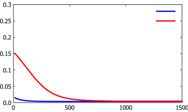
Figure 4: Learning curve of objective function $G(A)$ (blue line) and LLSFE based objective function $L(A)$ (19) (red line). Top: $x$ is Gaussian. Bottom: $x$ is Gaussian-mixture.

4.2 Combine with LLSFE

Now we use our estimator LLSFE to construct the empirical loss $\widehat{L}(A)$ to train a one-hidden-layer neural network (18). The setting of this experiment is same as that of Subsection 4.1 with $k=d=2$ for simplicity.

In the left panel of Figure. 4, we choose Gaussian input $x\sim\mathcal{N}(0,I_{d})$ so that the loss $G(A)$ coincides with $L(A)$ if the ground truth $\mathcal{S}_{4}(x)$ is known. We can see that using estimation error using $L(\cdot)$ operates close to that of the ground-truth $G(\cdot)$ In the right panel of Figure 4, we choose $x\sim 0.5\mathcal{N}({\bf 1}_{d},I_{d})+0.5\mathcal{N}(-{\bf 1}_{d},I_{d})$. In this case, $G(A)$ converges to a local minimum, thus incurring higher parameter error, whereas LLSFE-based objective function converges to the global minima very quickly. This confirms that when the data is not coming from a Gaussian distribution, it is critical to use properly matched estimator, which is provided by the proposed LLSFE approach.

5 Conclusion

Stochastic gradient descent is the dominant method for training neural networks. As SGD on the standard $\ell_{2}$ loss fails to converge to the true parameters of the “teacher” networks, from which the data is generated, there have been significant efforts to design a loss function with a good landscape. However, those new loss functions are typically tailored only for Gaussian distributions; a common assumption in theory of neural networks, but far from the real data.

To bridge this gap, we propose a new framework for designing the landscape for general smooth distributions. Using local likelihood density estimators, which can capture the local geometry of the probability density function, we introduce a novel estimator for score functions which $(i)$ involve higher-order derivatives of the input pdf and $(ii)$ are critical in the landscape design. This resolves one of the challenges in generalizing the Gaussian assumption, namely score function estimation.

There are other challenges in removing the Gaussian assumption in the analysis of more complicated networks, for example in Brutzkus and Globerson, (2017); Li and Yuan, (2017). Innovative analysis techniques are needed to complete the generalization of the Gaussian assumption, which is a promising direction for future research. Also, the time complexity of our approach is polynomial of the dimension of input, but the exact order of is unknown. Further improvement on time complexity could be a promising future research direction.

Appendix A Proof of Section 2

A.1 Proof of Theorem 1

Proof.

We rewrite the spectral norm error in terms of the polynomial representations (8) and (9) as

$$\|\widehat{\mathcal{S}_{m}}(x)-\mathcal{S}_{m}(x)\|_{\rm sp}\,$$ (23)

$$\leq \sum_{\lambda\in\Lambda_{m}}c_{m}(\lambda)\,\|{\rm sym}(\bigotimes_{j\in\lambda}\widehat{\mathcal{A}_{j}^{(p)}})-{\rm sym}(\bigotimes_{j\in\lambda}\mathcal{G}_{j})\|_{\rm sp}\,$$

$$\leq \sum_{\lambda\in\Lambda_{m}}c_{m}(\lambda)\,\|\bigotimes_{j\in\lambda}\widehat{\mathcal{A}_{j}^{(p)}}-\bigotimes_{j\in\lambda}\mathcal{G}_{j}\|_{\rm sp}\;,$$

where the last inequality comes from the fact that $\|{\rm sym}(\mathcal{T})\|_{\rm sp}\leq\|\mathcal{T}\|_{\rm sp}$. Then we study each term in (23). For simplicity of notation, denote the estimation error $\mathcal{E}_{j}^{(p)}\triangleq\widehat{\mathcal{A}_{j}^{(p)}}-\mathcal{G}_{j}$, then we have

$$\|\bigotimes_{j\in\lambda}\widehat{\mathcal{A}_{j}^{(p)}}-\bigotimes_{j\in\lambda}\mathcal{G}_{j}\|_{\rm sp}\,$$

$$= \|\bigotimes_{j\in\lambda}(\mathcal{E}_{j}^{(p)}+\mathcal{G}_{j})-\bigotimes_{j\in\lambda}\mathcal{G}_{j}\|_{\rm sp}\,$$

$$= \|\sum_{\nu\subset\lambda}\left(\left(\bigotimes_{j\in\nu}(\mathcal{E}_{j}^{(p)})\right)\otimes\left(\bigotimes_{j\in\lambda\setminus\nu}\mathcal{G}_{j}\right)\right)-\bigotimes_{j\in\lambda}\mathcal{G}_{j}\|_{\rm sp}\,$$

$$= \|\sum_{\nu\subset\lambda,\nu\neq\emptyset}\left(\left(\bigotimes_{j\in\nu}(\mathcal{E}_{j}^{(p)})\right)\otimes\left(\bigotimes_{j\in\lambda\setminus\nu}\mathcal{G}_{j}\right)\right)\|_{\rm sp}\,$$

$$\leq \sum_{\nu\subset\lambda,\nu\neq\emptyset}\|\left(\bigotimes_{j\in\nu}(\mathcal{E}_{j}^{(p)})\right)\otimes\left(\bigotimes_{j\in\lambda\setminus\nu}\mathcal{G}_{j}\right)\|_{\rm sp}\,$$

$$\leq \sum_{\nu\subset\lambda,\nu\neq\emptyset}\left(\,(\prod_{j\in\nu}\|\mathcal{E}_{j}^{(p)}\|_{\rm sp})\times(\prod_{j\in\lambda\setminus\nu}\|\mathcal{G}_{j}\|_{\rm sp})\,\right)\;.$$

Now we study the spectral norm of $\mathcal{E}_{j}^{(p)}$, which can be upper bounded by the Frobenius norm. Then by Lemma 2.1, we have,

$$\|\mathcal{E}_{j}^{(p)}\|_{\rm sp}\leq\|\mathcal{E}_{j}^{(p)}\|_{\mathcal{F}}=\sqrt{\sum_{i_{1},\dots,i_{j}}\left(\mathcal{E}_{j}^{(p)}\right)_{(i_{1},\dots,i_{j})}^{2}}\,$$ (25)

$$= O(d^{j/2}h^{p+1-j})+O_{p}(d^{j/2}(nh^{d+2j})^{-1/2}).$$

Since for any $j\leq m$, we have $h^{p+1-j}\to 0$ and $nh^{d+2j}\to\infty$ as $n\to\infty$. So for sufficiently large $n$, we have $\sum_{j\in\lambda}\|\mathcal{E}_{j}^{(p)}\|_{\rm sp}\leq 1$ with high probability. Then, plug it into (LABEL:eq:eq_2), we get

$$\|\bigotimes_{j\in\lambda}\widehat{\mathcal{A}_{j}^{(p)}}-\bigotimes_{j\in\lambda}\mathcal{G}_{j}\|_{\rm sp}\,$$ (26)

$$\leq \sum_{\nu\subset\lambda,\nu\neq\emptyset}\left(\,(\prod_{j\in\nu}\|\mathcal{E}_{j}^{(p)}\|_{\rm sp})\times\prod_{j\in\lambda\setminus\nu}C_{j}\,\right)\,$$

$$\leq C\sum_{\nu\subset\lambda,\nu\neq\emptyset}\prod_{j\in\nu}\|\mathcal{E}_{j}^{(p)}\|_{\rm sp}\,$$

$$= C\left(\prod_{j\in\lambda}(1+\|\mathcal{E}_{j}^{(p)}\|_{\rm sp})-1\right)\,$$

$$\leq C\left(\exp\{\sum_{j\in\lambda}\|\mathcal{E}_{j}^{(p)}\|_{\rm sp}\}-1\right)\,$$

$$\leq 2C\sum_{j\in\lambda}\|\mathcal{E}_{j}^{(p)}\|_{\rm sp}\,$$

$$= O(d^{j_{\rm max}/2}h^{p+1-j_{\rm max}})+O_{p}(d^{j_{\rm max}/2}(nh^{d+2j_{\rm max}})^{-1/2})$$

here constant $C=\max_{\nu}\prod_{j\in\lambda\setminus\nu}C_{j}$ and $j_{\rm max}=\max\{j:j\in\lambda\}$. The last inequality comes from the fact that $e^{y}-1\leq 2y$ for any $y\leq 1$. Since $\lambda$ is a partition of integer $m$, we have $j_{\rm max}\leq m$, and the equation holds if and only if $\lambda=\{m\}$. Therefore the only term in (23) that achieves $O(d^{m/2}h^{p+1-m})+O_{p}(d^{m/2}(nh^{d+2m})^{-1/2})$ is $\|\widehat{\mathcal{A}}_{m}^{(p)}-\mathcal{G}_{m}\|_{\rm sp}$, with $c_{m}(\lambda)=1$. Therefore, we complete the proof. ∎

Appendix B Proofs of Section 3

The key technical lemma behind our results is the Stein’s lemma and its generalizations which we present below.

Lemma B.1 (Stein et al., (1972)).

Let $x\sim\mathcal{N}(0,I_{d})$ and $g:\mathbb{R}^{d}\to\mathbb{R}$ be such that both $\mathbb{E}[\nabla g(x)]$ and $\mathbb{E}[g(x)x]$ exist and are finite. Then

$$\mathbb{E}[g(x)x]=\mathbb{E}[\nabla_{x}g(x)].$$ (27)

The following lemma generalizes Stein’s lemma to more general distributions and higher-order derivatives.

Lemma B.2 (Sedghi and Anandkumar, (2014)).

Let $m\geq 1$ and $\mathcal{S}_{m}(x)$ be defined as in (2). Then for any $g:\mathbb{R}^{d}\to\mathbb{R}$ satisfying some regularity conditions, we have

$$\mathbb{E}[g(x)\cdot\mathcal{S}_{m}(x)]=\mathbb{E}[\nabla_{x}^{(m)}g(x)].$$ (28)

The following theorem gives an alternate characterization of the loss function $L$ and is the key step in the proof of Theorem 2.

Theorem 4.

The loss function $L(\cdot)$ defined in (19) satisfies that

$$L(A) = \sum_{i\in[d]}w_{i}^{\ast}\mathbb{E}[g^{(4)}(\langle{a_{i}^{\ast}},{x}\rangle)]\sum_{j,k\in[d],j\neq k}\langle{a_{i}^{\ast}},{a_{j}}\rangle^{2}\langle{a_{i}^{\ast}},{a_{k}}\rangle^{2}\,$$ (29)

$$\;-\mu\sum_{i,j\in[d]}w_{i}^{\ast}\mathbb{E}[g^{(4)}(\langle{a_{i}^{\ast}},{x}\rangle)]\langle{a_{i}^{\ast}},{a_{j}}\rangle^{4}+\lambda\sum_{i\in[d]}(\left\|a_{i}\right\|-1)^{2}\;.$$

Proof.

Since $\eta$ is zero-mean and independent of $x$, we have that

$$\mathbb{E}[y\cdot\mathcal{S}_{m}(x)]=\sum_{i\in[k]}w_{i}^{\ast}\mathbb{E}[g(\langle{a_{i}^{\ast}},{x}\rangle\cdot\mathcal{S}_{m}(x))]\;,$$ (30)

∎

Putting $m=4$ in Lemma B.2, in view of (30), we obtain that

$$\mathbb{E}[y\cdot\mathcal{S}_{4}(x)]=\sum_{i\in[k]}w_{i}^{\ast}\mathbb{E}[g^{(4)}(\langle{a_{i}^{\ast}},{x}\rangle)](a_{i}^{\ast})^{\otimes 4}.$$ (31)

Thus for any fixed $a_{j},a_{k}$, we have

$$\mathbb{E}[y\cdot\mathcal{S}_{4}(x)(a_{j},a_{j},a_{k},a_{k})]=\mathbb{E}[y\cdot t_{1}(x)]\,$$

$$= \sum_{i\in[k]}w_{i}^{\ast}\mathbb{E}[g^{(4)}(\langle{a_{i}^{\ast}},{x}\rangle)]\langle{a_{i}^{\ast}},{a_{j}}\rangle^{2}\langle{a_{i}^{\ast}},{a_{k}}\rangle^{2},$$

$$\mathbb{E}[y\cdot\mathcal{S}_{4}(x)(a_{j},a_{j},a_{j},a_{j})]=\mathbb{E}[y\cdot t_{2}(x)]\,$$

$$= \sum_{i\in[k]}w_{i}^{\ast}\mathbb{E}[g^{(4)}(\langle{a_{i}^{\ast}},{x}\rangle)]\langle{a_{i}^{\ast}},{a_{j}}\rangle^{4}.$$ (33)

Now summing over $j,k$ finishes the proof.

B.1 Proof of Theorem 2

Proof.

The proof directly follows from Theorem 2.3 of Ge et al., (2017) and Theorem 4. ∎

B.2 Proof of Theorem 3

We formally state our assumptions for the finite sample landscape analysis below.

Assumption 3.

1. $\left\|x\right\|$ has exponentially decaying tails, i.e.

   $$\mathbb{P}\left[\left\|x\right\|^{2}\geq t\right]\leq K_{1}e^{-K_{2}t^{2}},\quad\forall t\geq 0,$$ (34)

   for some constants $K_{1},K_{2}>0$.

2. Let $l(x,y,A)$ be such that $L(A)=\mathbb{E}[l(x,y,A)]+\lambda\sum_{i\in[k]}(\left\|a_{i}\right\|^{2}-1)^{2}$. Then there exists a constant $K>0$ which is at most a polynomial in $d$ and a constant $p\in\mathbb{N}$ such that

   $$\left\|\nabla_{A}l(x,y,A)\right\| \leq K\left\|x\right\|^{p},$$

   $$\left\|\nabla^{2}_{A}l(x,y,A)\right\| \leq K\left\|x\right\|^{p},$$ (35)

   for all $A$ such that $\left\|A_{i}\right\|\leq 2$.

In order to establish that the gradient and the Hessian of $L$ are close to their finite sample counterparts, we first consider its truncated version $L_{T}$ defined as

$$L_{T}\triangleq\mathbb{E}[l(x,y,A)\mathbbm{1}_{E}],\quad E\triangleq\{\left\|x\right\|\leq R\},$$ (36)

where $R=Cd\log(1/\varepsilon)$ for some $\varepsilon<0$. It follows that $L_{T}$ is well behaved and exhibits uniform convergence of empirical gradients/Hessians to its population version Ge et al., (2017) for $A$ with bounded norm. Then Theorem 3 follows from showing that the gradient and the Hessian of $L_{T}$ are close to that of $L$ as well in this setting, which we prove in Lemma B.3. Next we combine this result with Lemma E.5 of Ge et al., (2017) which shows that $A$ with large row norms must also have large gradients and hence cannot be local minima. First we define $L_{T}$

Lemma B.3.

Let $L_{T}$ be defined as in (36) and Assumption 3 hold. Then for a sufficiently large constant $C$ and a sufficiently small $\varepsilon>0$, we have that

$$\left\|\nabla L(A)-\nabla L_{T}(A)\right\|_{2}\leq\varepsilon,$$ (37)

$$\left\|\nabla^{2}L(A)-\nabla^{2}L_{T}(A)\right\|_{2}\leq\varepsilon.$$ (38)

for all $A$ with row norm $\|A_{i}\|\leq 2$.

Proof.

We have that

$$\left\|\nabla L(A)-\nabla L_{T}(A)\right\|_{2}\,$$ (39)

$$= \left\|\mathbb{E}[\nabla l(x,y,A)(1-\mathbbm{1}_{E})]\right\|\,$$

$$\stackrel{{\scriptstyle(a)}}{{\leq}} \mathbb{E}[\left\|\nabla l(x,y,A)\right\|\mathbbm{1}\{\left\|x\right\|\geq R\}]\,$$

$$= \sum_{i\geq 0}\mathbb{E}[\left\|\nabla l(x,y,A)\right\|\mathbbm{1}\{\left\|x\right\|\in[2^{i}R,2^{i+1}R]\}]\,$$

$$\stackrel{{\scriptstyle(b)}}{{\leq}} \sum_{i\geq 0}K(2^{i+1}R)^{p}\mathbb{P}\left[\left\|x\right\|\geq 2^{i}R\right]\,$$

$$\leq \sum_{i\geq 0}K(2^{i+1}R)^{p}e^{-2^{i}R}\,$$

$$\stackrel{{\scriptstyle(c)}}{{\leq}} \sum_{i\geq 0}e^{-2^{i-1}R}\,$$

$$= \sum_{i\geq 0}\varepsilon^{Cd2^{i-1}}\,$$

$$\stackrel{{\scriptstyle(d)}}{{\leq}} \sum_{i\geq 0}\varepsilon/2^{i+1}=\varepsilon,$$

where $(a)$ follows from the Jensen’s inequality, $(b)$ follows from Assumption 3, $(c)$ follows from the fact that $K(2x)^{p}e^{-x}\leq e^{-x/2}$ for $x$ sufficiently large, and $(d)$ follows from choosing $C$ sufficiently large. Similarly for $\left\|\nabla^{2}L(A)-\nabla^{2}L_{T}(A)\right\|_{2}$. ∎

We are now ready to prove Theorem 3.

Proof.

Let $A$ be such that norms of all the rows are less than $2$. Then we have from Lemma B.3 that

$$\left\|\nabla L(A)-\nabla L_{T}(A)\right\|_{2}\leq\varepsilon/4,$$ (40)

$$\left\|\nabla^{2}L(A)-\nabla^{2}L_{T}(A)\right\|_{2}\leq\tau_{0}/4.$$ (41)

Notice that the gradient and Hessian of $l(x,y,A)\mathbbm{1}_{E}$ are bounded $\tau=\mathrm{poly}(d,1/\varepsilon)$ for some fixed polynomial $\mathrm{poly}$. Hence using the uniform convergence of the sample gradients/Hessians to their population counterparts (Ge et al.,, 2017, Theorem E.3), we have that

$$\left\|\nabla L_{T}(A)-\nabla\hat{L}_{T}(A)\right\|_{2}\leq\varepsilon/6,$$ (42)

$$\left\|\nabla^{2}L_{T}(A)-\nabla^{2}\hat{L}_{T}(A)\right\|_{2}\leq\tau_{0}/6,$$ (43)

whenever $N\geq\mathrm{poly}(d,1/\varepsilon)$, with high probability. Moreover, from standard concentration inequalities (such as multivariate Chebyshev) it follows that

$$\left\|\nabla\hat{L}(A)-\nabla\hat{L}_{T}(A)-(\nabla L(A)-\nabla L_{T}(A))\right\|_{2}\,$$

$$\leq \varepsilon/6,$$

$$\left\|\nabla^{2}\hat{L}(A)-\nabla^{2}\hat{L}_{T}(A)-(\nabla^{2}L(A)-\nabla^{2}L_{T}(A))\right\|_{2}\,$$

$$\leq \tau_{0}/6,$$ (45)

with high probability, whenever $N\geq\mathrm{poly}(d,1/\varepsilon)$. Hence, we obtain that

$$\left\|\nabla L(A)-\nabla\hat{L}(A)\right\|_{2}\leq\varepsilon/2,$$ (46)

$$\left\|\nabla^{2}L(A)-\nabla^{2}\hat{L}(A)\right\|_{2}\leq\tau_{0}/2.$$ (47)

If $A$ is such that there exists a row $A_{i}$ with $\left\|A_{i}\right\|\geq 2$, we have from (Ge et al.,, 2017, Lemma E.5) that $\langle{\nabla\hat{L}(A),A_{i}},{\geq}\rangle c\lambda\left\|A_{i}\right\|^{4}$ for a small constant $c$ and thus $A$ cannot be a local minimum for $\hat{L}$. Hence all local minima of $\hat{L}$ must have $\left\|A_{i}\right\|\leq 2$ and thus in view of (47) it follows that it also a $\varepsilon$-approximate local minima of $L$, or more concretely,

$$\left\|\nabla L(A)\right\|\leq\varepsilon,\quad\nabla^{2}L(A)\succcurlyeq-\tau_{0}I_{d}.$$ (48)

∎

B.3 Landscape design for $k<d$

In the setting where $k=d$ and the regressors $a_{1}^{\ast},\ldots,a_{d}^{\ast}$ are linearly independent, our loss functions $L_{4}(\cdot)$ can modified in a straightforward manner to arrive at the loss function $F(\cdot)$ defined in Appendix C.2 of Ge et al., (2017). Hence we have the same landscape properties as that of Theorem B.1 of Ge et al., (2017). The proof is exactly similar to that of our Theorem 2.

In a more geneal scenario where $k<d$ and the regressors $a_{1}^{\ast},\ldots,a_{d}^{\ast}$ are linearly independent, it turns out that our loss function $L_{4}(\cdot)$ can also be transformed to obtain the loss $\mathcal{F}(\cdot)$ in Appendix C.3 of Ge et al., (2017) to arrive at Theorem C.1 of Ge et al., (2017) in our setting. The proof is again similar.

References

- Andoni et al., (2014) Andoni, A., Panigrahy, R., Valiant, G., and Zhang, L. (2014). Learning polynomials with neural networks. In International Conference on Machine Learning, pages 1908–1916.
- Arora et al., (2014) Arora, S., Bhaskara, A., Ge, R., and Ma, T. (2014). Provable bounds for learning some deep representations. In International Conference on Machine Learning, pages 584–592.
- Boob and Lan, (2017) Boob, D. and Lan, G. (2017). Theoretical properties of the global optimizer of two layer neural network. arXiv preprint arXiv:1710.11241.
- Brutzkus and Globerson, (2017) Brutzkus, A. and Globerson, A. (2017). Globally optimal gradient descent for a convnet with gaussian inputs. arXiv preprint arXiv:1702.07966.
- Choromanska et al., (2015) Choromanska, A., Henaff, M., Mathieu, M., Arous, G. B., and LeCun, Y. (2015). The loss surfaces of multilayer networks. In Artificial Intelligence and Statistics, pages 192–204.
- Du and Lee, (2018) Du, S. S. and Lee, J. D. (2018). On the power of over-parametrization in neural networks with quadratic activation. arXiv preprint arXiv:1803.01206.
- Freeman and Bruna, (2016) Freeman, C. D. and Bruna, J. (2016). Topology and geometry of half-rectified network optimization. arXiv preprint arXiv:1611.01540.
- Fukunaga and Hostetler, (1975) Fukunaga, K. and Hostetler, L. (1975). The estimation of the gradient of a density function, with applications in pattern recognition. IEEE Transactions on information theory, 21(1):32–40.
- Gao et al., (2016) Gao, W., Oh, S., and Viswanath, P. (2016). Breaking the bandwidth barrier: Geometrical adaptive entropy estimation. In Advances in Neural Information Processing Systems, pages 2460–2468.
- Ge et al., (2018) Ge, R., Kuditipudi, R., Li, Z., and Wang, X. (2018). Learning two-layer neural networks with symmetric inputs. arXiv preprint arXiv:1810.06793.
- Ge et al., (2017) Ge, R., Lee, J. D., and Ma, T. (2017). Learning one-hidden-layer neural networks with landscape design. arXiv preprint arXiv:1711.00501.
- Goel and Klivans, (2017) Goel, S. and Klivans, A. (2017). Learning depth-three neural networks in polynomial time. arXiv preprint arXiv:1709.06010.
- Hillar and Lim, (2013) Hillar, C. J. and Lim, L.-H. (2013). Most tensor problems are np-hard. Journal of the ACM (JACM), 60(6):45.
- Hjort and Jones, (1996) Hjort, N. L. and Jones, M. (1996). Locally parametric nonparametric density estimation. The Annals of Statistics, pages 1619–1647.
- Hyvärinen, (2005) Hyvärinen, A. (2005). Estimation of non-normalized statistical models by score matching. Journal of Machine Learning Research, 6(Apr):695–709.
- Janzamin et al., (2014) Janzamin, M., Sedghi, H., and Anandkumar, A. (2014). Score function features for discriminative learning: Matrix and tensor framework. arXiv preprint arXiv:1412.2863.
- (17) Janzamin, M., Sedghi, H., and Anandkumar, A. (2015a). Beating the perils of non-convexity: Guaranteed training of neural networks using tensor methods. arXiv preprint arXiv:1506.08473.
- (18) Janzamin, M., Sedghi, H., Niranjan, U., and Anandkumar, A. (2015b). Feast at play: Feature extraction using score function tensors. In Feature Extraction: Modern Questions and Challenges, pages 130–144.
- Li and Yuan, (2017) Li, Y. and Yuan, Y. (2017). Convergence analysis of two-layer neural networks with relu activation. In Advances in Neural Information Processing Systems, pages 597–607.
- Liang et al., (2018) Liang, S., Sun, R., Li, Y., and Srikant, R. (2018). Understanding the loss surface of neural networks for binary classification. arXiv preprint arXiv:1803.00909.
- Livni et al., (2014) Livni, R., Shalev-Shwartz, S., and Shamir, O. (2014). On the computational efficiency of training neural networks. In Advances in Neural Information Processing Systems, pages 855–863.
- Loader et al., (1996) Loader, C. R. et al. (1996). Local likelihood density estimation. The Annals of Statistics, 24(4):1602–1618.
- Nguyen and Hein, (2017) Nguyen, Q. and Hein, M. (2017). The loss surface and expressivity of deep convolutional neural networks. arXiv preprint arXiv:1710.10928.
- Panigrahy et al., (2018) Panigrahy, R., Rahimi, A., Sachdeva, S., and Zhang, Q. (2018). Convergence results for neural networks via electrodynamics. In LIPIcs-Leibniz International Proceedings in Informatics, volume 94. Schloss Dagstuhl-Leibniz-Zentrum fuer Informatik.
- Sedghi and Anandkumar, (2014) Sedghi, H. and Anandkumar, A. (2014). Provable tensor methods for learning mixtures of classifiers. arXiv preprint.
- Soltanolkotabi et al., (2017) Soltanolkotabi, M., Javanmard, A., and Lee, J. D. (2017). Theoretical insights into the optimization landscape of over-parameterized shallow neural networks. arXiv preprint arXiv:1707.04926.
- Soudry and Hoffer, (2017) Soudry, D. and Hoffer, E. (2017). Exponentially vanishing sub-optimal local minima in multilayer neural networks. arXiv preprint arXiv:1702.05777.
- Stein et al., (1972) Stein, C. et al. (1972). A bound for the error in the normal approximation to the distribution of a sum of dependent random variables. In Proceedings of the Sixth Berkeley Symposium on Mathematical Statistics and Probability, Volume 2: Probability Theory. The Regents of the University of California.
- Stone, (1980) Stone, C. J. (1980). Optimal rates of convergence for nonparametric estimators. The annals of Statistics, pages 1348–1360.
- Swersky et al., (2011) Swersky, K., Buchman, D., Freitas, N. D., Marlin, B. M., et al. (2011). On autoencoders and score matching for energy based models. In Proceedings of the 28th international conference on machine learning (ICML-11), pages 1201–1208.
- Tian, (2017) Tian, Y. (2017). An analytical formula of population gradient for two-layered relu network and its applications in convergence and critical point analysis. arXiv preprint arXiv:1703.00560.
- Zhang et al., (2018) Zhang, X., Yu, Y., Wang, L., and Gu, Q. (2018). Learning one-hidden-layer relu networks via gradient descent. arXiv preprint arXiv:1806.07808.
- Zhong et al., (2017) Zhong, K., Song, Z., Jain, P., Bartlett, P. L., and Dhillon, I. S. (2017). Recovery guarantees for one-hidden-layer neural networks. arXiv preprint arXiv:1706.03175.