Simulation of Multiscale Hydrophobic Lipid Dynamics via Efficient Integral Equation Methods

Abstract

In this paper a mathematical model for long-range, hydrophobic attraction between amphiphilic particles is developed to quantify the macroscopic assembly and mechanics of a lipid bilayer membrane in solvents. The non-local interactions between amphiphilic particles are obtained from the first domain variation of a hydrophobicity functional, giving rise to forces and torques (between particles) that dictate the motion of both particles and the surrounding solvent. The functional minimizer (that accounts for hydrophobicity at molecular-aqueous interfaces) is a solution to a boundary value problem of the screened Laplace equation. We reformulate the boundary value problem as a second-kind integral equation (SKIE), discretize the SKIE using a Nyström discretization and ‘Quadrature by Expansion’ (QBX) and solve the resulting linear system iteratively using GMRES. We evaluate the required layer potentials using the ‘GIGAQBX’ fast algorithm, a variant of the Fast Multipole Method (FMM), yielding the required particle interactions with asymptotically optimal cost. Solving a mobility problem in Stokes flow is incorporated to obtain corresponding rigid body motion. The simulated fluid-particle systems exhibit a variety of multiscale behaviors over both time and length: Over short time scales, the numerical results show self-assembly for model lipid particles. For large system simulations, the particles form realistic configurations like micelles and bilayers. Over long time scales, the bilayer shapes emerging from the simulation appear to minimize a form of bending energy.

31A10, 35A15, 92C05

1 Introduction

In recent years, researchers have developed various macroscopic continuum formulations and a number of numerical methods for calculating energy minimizing and time-dependent shapes of lipid bilayer membranes, vesicles and red blood cells. While the Helfrich free energy of a lipid bilayer membrane assumes an infinitely thin membrane thickness [74, 33], many other continuum models incorporate more lipid physics [2, 6, 61] and membrane structures [12, 13, 21, 28, 43]. These refined continuum formulations are in principle capable of capturing topological changes of a lipid bilayer membrane, such as membrane fusion and fission. However, no simulations of membrane fusion or fission based on these refined formulations are available in the literature (to our knowledge), possibly due to the numerical challenges to efficiently and accurately resolve structures on the scale of membrane thickness.

Changes in topology of bilayer membranes, as occur in bilayer membrane fusion, pore formation and protein insertion, for example, involve the introduction of a hydrophobic fissure in the normally intact monolayer surface. Due to the relatively large tension of a hydrocarbon-water interface, the energy of a hydrophobic fissure can dominate the membrane’s elastic energy, making it necessary to also take into account local interactions at the molecular level [22, 14]. Moreover, in many subcellular structures, membrane energies are dominant in high curvature regions only a few lipids wide [34, 82].

Based on these observations, we focus on topological changes with mesoscopic interactions in a semi-continuum framework where the lipids are coarse-grained into amphiphilic Janus-type particles while their interactions with each other and the solvents are described at a continuum level. This hybrid approach provides a bridge from microscopic molecular formulation to macroscopic continuum description of a lipid bilayer membrane. Furthermore, the continuum limit of our hybrid mesoscopic model may facilitate efficient numerical algorithms for simulating fusion/fission of lipid bilayer membranes of physically relevant membrane size and dynamic duration.

Modern molecular dynamics (MD) simulators (such as MARTINI [52] andLAMMPS [66]) have the advantage in that they resolve all relevant molecular details, and have been widely employed to simulate fully atomistic or coarse-grained lipid bilayer membrane based on pairwise interactions [11, 23, 37, 38, 52, 81]. Traditionally, MD numerical methods use explicit fluid particles such as coarse-grained water molecules and pairwise Lennard-Jones interactions. There is the disadvantage, though, that an enormous number of water molecules and long computation time are needed in MD simulations, and it remains a great challenge to compute the hydrodynamic interactions of the lipid membrane at micron size for durations long enough to make physical predictions. One way to mitigate long computation time is to compute hydrodynamic interactions using an implicit solvent and Stokesian dynamics [4].

In the present work, we propose a novel approach to lipid-lipid interactions called the hydrophobic attraction domain functional (HADF). Let $\displaystyle\Omega$ be an open, exterior domain in $\displaystyle\mathbb{R}^{n}$ representing water surrounding a collection of amphiphilic particles, e.g. lipids. For dispersed particles, the energy associated with hydrophobic interfaces behaves as a surface energy. When nearby, particles decrease their energy by aggregating and sequestering their hydrophobic interfaces from water. These interactions are well-described by the Ginzburg-Landau-type domain functional

(1) $$\Phi(\Omega,f)=\gamma\min_{u\in\mathcal{A}}I[u],$$

where

(2) $$I[u]=\int_{\Omega}\rho|\nabla u|^{2}+\rho^{-1}u^{2}\,dx.$$

Here $\displaystyle\mathcal{A}=\{u\in W^{1,2}(\Omega):u=f\text{ on }\Sigma\}$ is the admissible class and $\displaystyle f$ with range $\displaystyle[0,1]$ is the hydrophobicity label for the water-particle interface $\displaystyle\Sigma=\partial\Omega.$ The parameter $\displaystyle\gamma>0$ is interfacial tension. Its value in bilayers has been widely investigated in both numerical and theoretical studies [18, 24, 56, 65]. For a Lipschitz domain $\displaystyle\Omega$ and for $\displaystyle f$ the trace of a function in $\displaystyle W^{1,2}(\Omega)$ [19], the existence of a unique minimizer to Eq. 1 is a straightforward consequence of the closest point theorem [46].

The scalar function $\displaystyle u$ of Eq. 1 models disruption in the hydrogen bonding network [17, 53]. For a point $\displaystyle x\in\Sigma$ representing a hydrophobic interface, water mobility is restricted and there $\displaystyle u(x)=f(x)=1.$ Conversely, $\displaystyle u(x)=f(x)=0$ at a point $\displaystyle x\in\Sigma$ representing a hydrophilic interface where water mobility is unrestricted. In the water region, $\displaystyle u$ in Eq. 1 is a solution to the boundary value problem (BVP) of the screened Laplace equation:

(3) $$\begin{cases}-\rho^{2}\Delta u+u=0&\text{ in }\Omega,\\ u(x)=f(x)&\text{ on }\Sigma,\\ u(x)\to 0,&\text{ as }x\to\infty.\end{cases}$$

Solutions $\displaystyle u$ of Eq. 3 have a boundary layer of thickness $\displaystyle\rho>0.$ Thus disruption in hydrogen bonding modeled by Eq. 3 extends into the bulk with characteristic distance $\displaystyle\rho$ [15, 54].

The hydrophobic force is the first variation of the functional $\displaystyle\Phi$ with respect to the shape of the domain $\displaystyle\Omega.$ The challenge in the present work is to compute the hydrophobic force between several bodies of arbitrary shape and configuration. Section 2 carries out the variation for rigid body motions, and this reduces to a set of boundary integrals for the hydrophobic forces and torques. For simulations, we utilize a boundary condition $\displaystyle f$ representing surface portions of lipid tail and lipid head, and we adopt an excluded volume repulsion to avoid particle collisions in the many-body simulations. As an illustration, Fig. 1 shows the self-assembly process for three Janus-type particles in a viscous fluid.

An important feature of the model is that the potential $\displaystyle\Phi$ and its intermolecular forces and torques, in contrast to that of coarse-grained theories, do not arise from any pairwise potentials (see Appendix A). To leading order, the attraction between particle pairs predicted by Eq. 1 is in accord with experimental force-distance curves [17, 48, 54]. The functional Eq. 1, however, requires modification for account for sub-nanometer force oscillations observed in experiment, e.g. through the inclusion of higher order terms. Nevertheless, the HADF captures the essential features of amphiphile self-assembly, and the variational calculations and numerical methods generalize to more complicated domain functionals.

An essential principle for molecular or particle based approaches is to ensure that the total free energy accounting for lipid-lipid and lipid-water interactions gives rise to an equivalent elastic characterization of membranes as determined by experimental measurements [77, 78]. Section 3 examines the elasticity of bilayer particle configurations. We obtain physical quantities such as bending modulus, tilt modulus and stretching modulus by setting up corresponding equilibrium simulations from continuum theory [41, 58, 76].

Section 4 formulates the mobility problem to calculate hydrodynamics from the hydrophobic stress. The dynamics for many-particle simulations yield physically reasonable time scales and configurations. For example, we can track the particle dynamics over the nanosecond range needed for rapid particle self assembly, up to the microseconds range where bilayer and micelle shapes evolve over a slower time scale [69, 70].

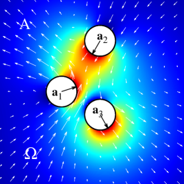
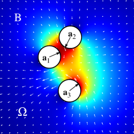
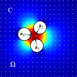
Figure 1: The figure illustrates hydrophobic attraction of amphiphiles in a zero-Reynolds number fluid. The black arrows are the directors $\displaystyle\mathbf{d}_{i}$ of the particles centered at $\displaystyle\mathbf{a}_{i}$, $\displaystyle i=1,2,3$. The white arrows are the fluid velocity. The color map has dark blue is for $\displaystyle u=0$ (lipid heads) and dark red is for the hydrophobic interface $\displaystyle u=1$ (lipid tails). Activity, shown as pseudo-color shading in the figure, extends from the hydrophobic interface into the bulk. Going from panels A to B, particles $\displaystyle\mathbf{a}_{1}$ and $\displaystyle\mathbf{a}_{2}$ come together and $\displaystyle\mathbf{a}_{3}$ rotates counterclockwise. In panel C, the particles sequester activity to a single hydrophobic core.

Calculating the particle dynamics requires rapid, on-the-fly solution of Eq. 3. In Section 5, we present a new SKIE formulation for the boundary value problem Eq. 3, derived from a representation of the solution in which the unknowns are only on the boundary $\displaystyle\Sigma$. In Section 6, we describe an approach to applying a recently developed QBX-FMM scheme for discretizing the SKIE accurately and adaptively, solving the resulting linear system and evaluating the desired physical quantities afterwards accurately and rapidly. The resulting scheme has linear complexity with an optimal number of unknowns for the simulation of particle dynamics at each time step. To compare the computational cost against MD simulations, even solvent free coarse-grained models have at least $\displaystyle O(N^{2})$ complexity in the number of particle $\displaystyle N$ [11, 60].

2 Intermolecular Forces and Torques

We calculate the first variation of $\displaystyle\Phi$ with respect to rigid body deformations [1, 73]. Consider $\displaystyle N$-many, rigid particles represented by disjoint, bounded, closed regions $\displaystyle P_{1},P_{2},\dots,P_{N}$ in $\displaystyle\mathbb{R}^{n},$ $\displaystyle n=2,3$. The water region (the exterior domain) and particle-water interface are

(4) $$\Omega=\mathbb{R}^{n}\setminus\bigcup_{i=1}^{N}P_{i},\quad\Sigma=\bigcup_{i=1}^{N}\partial P_{i},$$

respectively. Throughout, $\displaystyle\nu$ denotes the unit outward normal to $\displaystyle\Omega$, and $\displaystyle\nu_{i}$ denotes the unit outward normal to $\displaystyle P_{i}$. Note that $\displaystyle\nu$ and $\displaystyle\nu_{i}$ have opposite orientation, as illustrated in Figure 2. Suppose that $\displaystyle u$ is the solution to the screened Laplace BVP Eq. 3 with the material label $\displaystyle f$. Then the force $\displaystyle\mathbf{F}_{i}$ and torque $\displaystyle\tau_{i}^{0}$ acting on particle $\displaystyle P_{i}$ are

(5) $$\mathbf{F}_{i}=\int_{\partial P_{i}}\mathbf{T}\cdot\nu_{i}\,dS,\quad\tau_{i}^{0}=\int_{\partial P_{i}}\mathbf{r}_{0}\times(\mathbf{T}\cdot\nu_{i})\,dS,$$

where

(6) $$\mathbf{T}=\gamma\rho^{-1}u^{2}\mathbf{I}+2\rho\gamma(\tfrac{1}{2}|\nabla u|^{2}\mathbf{I}-\nabla u\otimes\nabla u),$$

is the hydrophobic stress and $\displaystyle\mathbf{r}_{0}$ is the position vector relative to the origin $\displaystyle\mathbf{0}$. To ensure that Eq. 5 is well-defined and to guarantee differentiability of the domain functional, we that $\displaystyle\Omega$ is a $\displaystyle C^{2,\alpha}$ domain and that $\displaystyle f=\tilde{f}$ on $\displaystyle\Sigma$ for some $\displaystyle\tilde{f}\in C^{2,\alpha}(\overline{\Omega})$.

To compare $\displaystyle\Phi(\Omega,f)$ against that of competing domains, consider a one-parameter family of rigid transformations

(7) $$\mathbf{x}_{i}(\mathbf{X},\epsilon)=\mathbf{c}_{i}(\epsilon)+\mathbf{Q}_{i}(\epsilon)\mathbf{X},$$

parametrized by $\displaystyle\epsilon\in\mathbb{R}$. The vector $\displaystyle\mathbf{c}_{i}(\epsilon)$ and tensor $\displaystyle\mathbf{Q}_{i}(\epsilon)$ give the displacement and rotation of the particle $\displaystyle P_{i}$, $\displaystyle i=1,\dots,N$, relative to the origin. They satisfy $\displaystyle\mathbf{c}_{i}(0)=\mathbf{0}$ and $\displaystyle\mathbf{Q}_{i}(0)=I$ so that $\displaystyle\mathbf{x}_{i}(\mathbf{X},0)$ is the identity transformation; $\displaystyle\mathbf{Q}_{i}(\epsilon)\mathbf{Q}_{i}^{T}(\epsilon)=I$ for all $\displaystyle\epsilon$. The distance between $\displaystyle P_{i}$ and $\displaystyle P_{j}$ is positive whenever $\displaystyle i\neq j$. Therefore, for $\displaystyle\epsilon$ in an open interval about $\displaystyle 0$, let

(8) $$\Omega_{\epsilon}=\mathbb{R}^{n}\setminus\bigcup_{i=1}^{N}\mathbf{x}_{i}(P_{i},\epsilon),\quad\Sigma_{\epsilon}=\partial\Omega_{\epsilon},\quad f_{\epsilon}(\mathbf{x}_{i}(\mathbf{X},\epsilon))=f(\mathbf{X}),\quad\mathbf{X}\in\partial P_{i}.$$

Finally, let $\displaystyle u_{\epsilon}(x)$ be the one-parameter family of solutions to the perturbed boundary value problem of screened Laplace equation

(9) $$-\rho^{2}\Delta u_{\epsilon}+u_{\epsilon}=0\text{ in }\Omega_{\epsilon},\quad u_{\epsilon}=f_{\epsilon}\text{ in }\Sigma_{\epsilon},\quad u_{\epsilon}\to 0\text{ as }x\to\infty.$$

The domain $\displaystyle\Omega_{\epsilon}$ and boundary $\displaystyle\Sigma_{\epsilon}$ are the water region and water-molecule interface after transforming each particle according to its rigid motion Eq. 7 (see Fig. 2). For $\displaystyle x\in\Omega$, let

$$\dot{u}(x)=\frac{d}{d\epsilon}u_{\epsilon}(x)\Big{|}_{\epsilon=0},$$

and extend $\displaystyle\dot{u}$ continuously to $\displaystyle\overline{\Omega}$. Due to Eq. 8, we have the transport identity

(10) $$\dot{u}+\nabla u\cdot\dot{\mathbf{x}}=0\mbox{ on }\Sigma,$$

where $\displaystyle\dot{\mathbf{x}}(\mathbf{X})=\frac{d\mathbf{x}_{i}}{d\epsilon}(\mathbf{X},0)$ whenever $\displaystyle\mathbf{X}\in P_{i}$. (Note, however, that the values of $\displaystyle\dot{u}$ in $\displaystyle\Omega$ are determined by the BVP Eq. 9, and therefore do not generally satisfy this transport relation.)

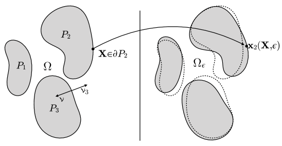
Figure 2: On the left are three particles $\displaystyle P_{1},$ $\displaystyle P_{2}$ and $\displaystyle P_{3}$ forming the exterior domain $\displaystyle\Omega$. Rigid transformation of each particle (right panel) leads to the perturbed exterior domain $\displaystyle\Omega_{\epsilon}$ and changes in the relative positions of the material label $\displaystyle f_{\epsilon}$, resulting in variations in the hydrophobic potential $\displaystyle\Phi$.

Applying the Reynolds transport theorem [47], we obtain

(11) $$\frac{d}{d\epsilon}\Phi(\Omega_{\epsilon},f_{\epsilon})\Big{|}_{\epsilon=0}=\gamma\frac{d}{d\epsilon}\left(\int_{\Omega_{\epsilon}}\rho|\nabla u_{\epsilon}|^{2}+\rho^{-1}u_{\epsilon}^{2}\,dx\right)\Big{|}_{\epsilon=0}$$

$$=\gamma\int_{\Omega}2\rho\nabla u\cdot\nabla\dot{u}+2\rho^{-1}u\dot{u}\,dx+\gamma\int_{\Sigma}\left(\rho|\nabla u|^{2}+\rho^{-1}u^{2}\right)\dot{\mathbf{x}}\cdot\nu\,dS.$$

Integration by parts then gives

(12) $$\displaystyle\frac{d}{d\epsilon}\Phi(\Omega_{\epsilon},f_{\epsilon})\Big{|}_{{\epsilon}=0}=\gamma\int_{\Sigma}\left(\rho|\nabla u|^{2}+\rho^{-1}u^{2}\right)\dot{\mathbf{x}}\cdot\nu-2\rho\nabla u\cdot\nu\dot{u}\,dS.$$

Due to the minimality condition $\displaystyle-\rho^{2}\Delta u+u=0$, the interior values of $\displaystyle\dot{u}$ do not enter Eq. 12. Based on Eq. 10 and the fact that $\displaystyle\nu$ and $\displaystyle\nu_{i}$ have opposite orientation,

$$\displaystyle\frac{d}{d\epsilon}\Phi(\Omega_{\epsilon},f_{\epsilon})\Big{|}_{{\epsilon}=0} \displaystyle=\gamma\sum_{i=1}^{N}\int_{\partial P_{i}}-\left(\rho|\nabla u|^{2}+\rho^{-1}u^{2}\right)\nu_{i}\cdot\dot{\mathbf{x}}_{i}(0)+2\rho\nabla u\cdot\nu_{i}\nabla u\cdot\dot{\mathbf{x}}_{i}(0)\,dS$$

$$\displaystyle=\gamma\sum_{i=1}^{N}\int_{\partial P_{i}}\dot{\mathbf{x}}_{i}(0)\cdot\left[-\rho^{-1}u^{2}\mathbf{I}+2\rho(\nabla u\otimes\nabla u-\tfrac{1}{2}|\nabla u|^{2}\mathbf{I})\right]\cdot\nu_{i}\,dS$$

$$\displaystyle=-\sum_{i=1}^{N}\int_{\partial P_{i}}(\dot{\mathbf{c}}_{i}(0)+\dot{\mathbf{Q}}_{i}(0)\mathbf{r}_{0})\cdot\mathbf{T}\cdot\nu_{i}\,dS$$

(13) $$\displaystyle=-\sum_{i=1}^{N}\left(\dot{\mathbf{c}}_{i}(0)\cdot\mathbf{F}_{i}+\mathbf{w}_{i}\cdot\tau_{i}^{0}\right),$$

where $\displaystyle\mathbf{w}_{i}=\langle w_{1}^{i},w_{2}^{i},w_{3}^{i}\rangle$ is the axial vector for the skew symmetric tensor $\displaystyle\dot{\mathbf{Q}}_{i}(0)$. In the second to last equation, the minus sign makes the force act in the negative direction of the potential gradient. This establishes Eq. 5 and Eq. 6.

In the formulation Eq. 7, the rigid motions are independent. Consider the case when the rigid motions are uniform, that is, $\displaystyle\mathbf{c}_{i}(\epsilon)=\mathbf{c}(\epsilon)$and $\displaystyle\mathbf{Q}_{i}(\epsilon)=\mathbf{Q}(\epsilon)$ for all $\displaystyle i=1,\dots,N$. Then the solution to the perturbed BVP (8, 9) satisfies

(14) $$u_{\epsilon}(\mathbf{c}(\epsilon)+\mathbf{Q}(\epsilon)\mathbf{X})=u(\mathbf{X}).$$

It follows that $\displaystyle\Phi(\Omega_{\epsilon},f_{\epsilon})=\Phi(\Omega,f)$ for all $\displaystyle\epsilon$ and, by Eq. 13, that

(15) $$\sum_{i=1}^{N}\dot{\mathbf{c}}(0)\cdot\mathbf{F}_{i}+\mathbf{w}\cdot\tau_{i}^{0}=-\frac{d}{d\epsilon}\Phi(\Omega_{\epsilon},f_{\epsilon})\Big{|}_{\epsilon=0}=-\frac{d}{d\epsilon}\Phi(\Omega,f)\Big{|}_{\epsilon=0}=0.$$

Here, $\displaystyle\mathbf{w}=\langle w_{1},w_{2},w_{3}\rangle$ is the axial vector for $\displaystyle\dot{\mathbf{Q}}(0)$. Since $\displaystyle\dot{\mathbf{c}}(0)$ and $\displaystyle\mathbf{w}$ are arbitrary, we have

(16) $$\sum_{i=1}^{N}\mathbf{F}_{i}=\mathbf{0},\quad\sum_{i=1}^{N}\tau_{i}^{0}=\mathbf{0}.$$

In other words, the net hydrophobic interaction is force and torque free.

2.1 Simulations

For the simulations in this paper, the $\displaystyle P_{1},\dots,P_{N}$ are two-dimensional Janus-type particles. The direction vector $\displaystyle\mathbf{d}_{i}=\langle\cos\theta_{i},\sin\theta_{i}\rangle$ specifies orientation and $\displaystyle\mathbf{a}_{i}$ is the particle position (e.g. the center of mass, Fig. 1). The particle shapes are ellipses with semi-major and semi-minor axes $\displaystyle a_{i}$ and $\displaystyle b_{i},$ respectively. In the case of lipids, $\displaystyle 2a_{i}$ represent lipid length and major axis is parallel to the director and hydrocarbon tail.

The material label for the Janus-type particle takes the form

(17) $$f(\mathbf{x})=1-\sin^{p}(\theta),\quad\mathbf{x}\in\partial P_{i},$$

where $\displaystyle\theta$ is the angle formed by $\displaystyle\mathbf{x}-\mathbf{a}_{i}$ and $\displaystyle\mathbf{d}_{i}.$ Accordingly, there is a smooth transition in hydrophobicity across the particle [51], with the boundary portion in the direction $\displaystyle\mathbf{d}_{i}$ modeling a hydrophobic tail and the opposite boundary portion modeling a hydrophilic head. The size of the hydrophobic region grows with the even integer parameter $\displaystyle p.$ Finally,

(18) $$\tau_{i}=\tau_{i}^{0}-\mathbf{a}_{i}\times\mathbf{F}_{i}$$

is the two-dimensional (scalar) torque about the position $\displaystyle\mathbf{a}_{i}$.

For small but fixed separations between particles, our numerical scheme accurately resolve the field $\displaystyle u$ without an undue cost increase due to refinement; we postpone a detailed discussion of the method and involved cost to Section 6. Dynamically, the forces Eq. 5 bring the coarse-grained lipid particles into contact. An excluded volume repulsion prevents near-contact between particles [64]. For two circular particles, the interaction is

(19) $$\mathbf{F}^{\mathrm{rep}}_{ij}=c_{0}\frac{q}{(|\mathbf{a}_{i}-\mathbf{a}_{j}|-(b_{i}+b_{j}))^{q+1}}\frac{\mathbf{a}_{i}-\mathbf{a}_{j}}{|\mathbf{a}_{i}-\mathbf{a}_{j}|},\quad i\neq j.$$

We fix the order $\displaystyle q=3$ ($\displaystyle q=4$ in three-dimensions) and use the parameter $\displaystyle c_{0}$ to control the strength of repulsion. For ellipses of eccentricity close to zero, we approximate the excluded volume repulsion using three circular particles placed along the major axes, as described in Supplementary Material, Section S1. In the sequel,

(20) $$\mathbf{F}^{\mathrm{rep}}_{i},\quad\tau_{i}^{\mathrm{rep}},\quad\Phi_{\mathrm{rep}},$$

denote the excluded volume force, torque and repulsion potential, respectively. The total potential that includes hydrophobic attraction and steric repulsion is

(21) $$\Phi_{\mathrm{Total}}=\Phi+\Phi_{\mathrm{rep}}.$$

For the simulations, we assume translation invariance in the $\displaystyle z$-direction. Figures 5 and 8 give values in $\displaystyle\mathrm{k_{B}T}$ per length since the two-dimensional simulations are for the cross-section of a three-dimensional bilayer. All other physical parameters correspond to their usual three-dimensional value.

We use $\displaystyle 2a_{i}=2.5$ nm as a representative phospholipid length [3], the screening length $\displaystyle\rho=2.5$ nm [17, 48, 63, 35, 76], and $\displaystyle c_{0}=0.5$ pN nm⁴ for the inter-particle repulsion. Bilayers containing different single pure components give various interfacial tension $\displaystyle\gamma$ values which are within the range of $\displaystyle 0.7$ – $\displaystyle 5.3$ pN nm^-1 [45, 65]. We find that the mechanical moduli calculated from our simulation data are in good agreement with results in the experimental literature when the interfacial tension $\displaystyle\gamma=4.1$ pN nm${}^{-1}.$ Coincidentally, this value corresponds to a specific lipid composition DPoPC:SM:Chol in bilayer membrane [24, Table 1].

Our experiences show that the computational cost to maintain the same numerical accuracy in solving the boundary value problem (3) grows only moderately when going from circular to elliptical model particles. For instance, ellipses with $\displaystyle a_{i}/b_{i}=3$ require 60 % more grid points than for $\displaystyle a_{i}/b_{i}=1.$ At the same time, ellipses afford flexibility in terms of dimensions that determine physical properties of bilayer. However, we remark that rather than representing a physical lipid or collection of lipids, the model particle discretizes the mean lipid position and orientation but without the mesh associated with finite element methods, for example [2, 72]. Similarly, the gap region between neighboring particles indicates a hydrophobic zone and not an intervening water.

3 Bilayer Elasticity

We compare our two-dimensional equilibrium configurations to those found in membrane continuum mechanics. In large particle number HADF simulations, particles bring opposing hydrophobic regions into contact, forming two abutting monolayers of a bilayer. Continuum theory describes monolayers using a director field $\displaystyle\mathbf{d}$ to track lipid orientations, along with a field $\displaystyle\mathbf{n}$ given by the monolayer surface normal (Figure 3A), and quantifies monolayer energy using a Helfrich Hamiltonian

(22) $$\int_{\mathcal{C}}\tfrac{1}{2}k_{\mathrm{B}}\left[\left(\operatorname{Div}\mathbf{d}+k_{0}\right)^{2}-k_{0}^{2}\right]+\tfrac{1}{2}k_{\theta}|\mathbf{d}\times\mathbf{n}|^{2}\,ds.$$

The curve $\displaystyle\mathcal{C}$ tracks the cross-section of the monolayer neutral surface. The integrand in Eq. 22 contains the splay distortion $\displaystyle\operatorname{Div}\mathbf{d}$ with bending modulus $\displaystyle k_{\mathrm{B}}$, and the tilt deformation $\displaystyle\mathbf{d}\times\mathbf{n}$ with tilt modulus $\displaystyle k_{\theta}$ [57]. The parameter $\displaystyle k_{0}$ is spontaneous curvature [71, 42, 75]. Since we are assuming translational invariance in the $\displaystyle z$-direction, the twist $\displaystyle\operatorname{Curl}\mathbf{d}$ and saddle-splay $\displaystyle\det\mathsf{D}$ distortions are absent from [33, 76], and Eq. 22 behaves as an energy density per length.

Consider a planar bilayer subject to a uniform vertical load. The bilayer is clamped and horizontal at one end and the restoring force of bending in the free part of the bilayer opposes the load. Taking $\displaystyle\mathbf{d}$ parallel to $\displaystyle\mathbf{n}$ and assuming a small deformation gives the appropriate functional

(23) $$\int_{0}^{L}k_{\mathrm{B}}(y^{\prime\prime})^{2}-ky\,dx,\quad y(0)=y^{\prime}(0),$$

where $\displaystyle y(x)$ is the height function for the bilayer midplane (Figure 3A, dashed curve), $\displaystyle\operatorname{Div}\mathbf{d}=\pm y^{\prime\prime}$ and $\displaystyle k$ is the load strength. The summation of the monolayer energies Eq. 22 with opposite normals leads to the cancelation of the spontaneous curvature terms in Eq. 23.

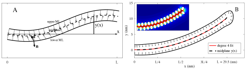
Figure 3: Panel A depicts a bilayer, with its upper and lower monolayers (solid curves) and midplane (dashed curve). The director field $\displaystyle\mathbf{d}$ points in the direction of the lipid tails and the normal $\displaystyle\mathbf{n}$ points outward from bilayer core. When deformations and tilt are small ($\displaystyle|y^{\prime}|\ll 1$, $\displaystyle|\mathbf{d}\times\mathbf{n}|\ll 1$) energy is quantified in terms of the midplane has the height function $\displaystyle y(x).$ Panel B has the equilibrium configuration Janus-type amphiphilic particles with uniform loading and a clamped boundary condition. Fitting Eq. 25 to the midplane (dashed curve) yields the bending modulus $\displaystyle k_{\mathrm{B}}=8.51$ $\displaystyle\mathrm{k_{B}T}.$ In Panel B (inset), enumerating counterclockwise from the bottom left, particles satisfy $\displaystyle x_{1}=0,$ $\displaystyle x_{16}=1.5$, $\displaystyle\theta_{1}=\pi/2,$ $\displaystyle\theta_{16}=-\pi/2$ and $\displaystyle y_{1}=0.$ The parameters are $\displaystyle\gamma=4.1$ pN nm^-1, $\displaystyle\rho=2.5$ nm, $\displaystyle c_{0}=0.5$ pN nm^-4 and $\displaystyle k=0.0116$ pN nm${}^{-2}.$ The ellipses have $\displaystyle a_{i}=1.25$ nm and $\displaystyle b_{i}=0.8$ nm.

Minimizers of Eq. 23 satisfy the boundary value problem

(24) $$2k_{\mathrm{B}}y^{(4)}=k,\quad y(0)=y^{\prime}(0)=y^{\prime\prime}(L)=y^{(3)}(L)=0.$$

We find the solution

(25) $$y(x)=\frac{kL^{4}}{2k_{\mathrm{B}}}\left[\frac{1}{24}\left(\frac{x}{L}\right)^{4}-\frac{1}{12}\left(\frac{x}{L}\right)^{3}+\frac{1}{4}\left(\frac{x}{L}\right)^{2}\right].$$

Thus, we can determine $\displaystyle k_{\mathrm{B}}$ from curves of the form Eq. 25 whenever $\displaystyle L$ and $\displaystyle k$ are given.

The inset in Figure 3B shows a HADF equilibrium configuration used to determine $\displaystyle k_{\mathrm{B}}.$ The $\displaystyle N=30$ particles minimize the modified functional

(26) $$\Phi_{\mathrm{Total}}-\sum_{i=1}^{N}\tilde{k}y_{i},$$

where the $\displaystyle\tilde{k}=Lk/N$ is the discrete load strength coming from quadrature of the integral Eq. 23 with $\displaystyle N$ many particles. To achieve minimality, the particles start in the shape of a flat bilayer, and then migrate upward following steepest gradient for Eq. 26.

The main figure in Figure 3B depicts the monolayer neutral surface (solid curve), midplane (dashed curve) and the lipid directors interpolated from the discrete particle positions and orientations (of the inset). The directors are everywhere normal to the neutral surface and the deformations are small. This justifies applying the zero-tilt, small-deformation solution Eq. 25. Fitting a 4th degree polynomial to the midplane curve (Figure 3B, red curve) supplies the coefficient $\displaystyle(kL^{4}/2k_{\mathrm{B}})$ of Eq. 25. Combining the coefficient with simulation values for $\displaystyle L$ and $\displaystyle k$ (Figure 3B, caption) yields $\displaystyle k_{\mathrm{B}}=8.51$ $\displaystyle\mathrm{k_{B}T}.$ This value for the bending modulus is for ellipses using $\displaystyle p=6$ in the hydrophobicity boundary condition Eq. 17. To assess how bilayer rigidity depends on the material label, we considered the energy minimization with $\displaystyle p=2,$ which gave $\displaystyle k_{\mathrm{B}}=13.54$ $\displaystyle\mathrm{k_{B}T}.$ We conclude that under HADF, particle configurations behave like an elastic material. The associated bending modulus grows with symmetry in the hydrophobic surface label, e.g. $\displaystyle k_{\mathrm{B}}$ was largest for $\displaystyle p=2$ where the label is symmetric across $\displaystyle\theta=\pi/2.$

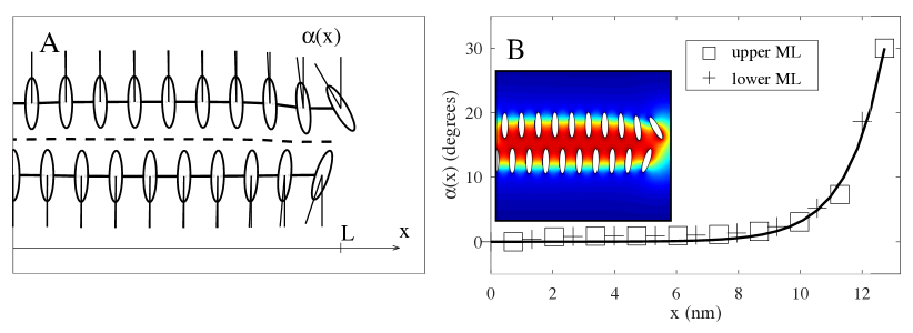
Figure 4: The monolayers in panel A are flat and tilt is nonzero. The horizontal coordinate $\displaystyle x$ runs between 0 and the length of bilayer, $\displaystyle L,$ and the function $\displaystyle\alpha(x)$ measure the angle between $\displaystyle-\mathbf{d}$ and the unit normal. The boundary conditions for Eq. 27 are $\displaystyle\alpha_{0}=0^{\circ}$ and $\displaystyle\alpha_{1}=30^{\circ}.$ In panel B, the $\displaystyle+$ and $\displaystyle\square$ symbols are the angles at the particle centers. The parameters are $\displaystyle\gamma=4.1$ pN nm^-1, $\displaystyle\rho=2.5$ nm, $\displaystyle c_{0}=0.5$ pN nm^-4, and $\displaystyle k=0.0116$ pN nm${}^{-2}.$ The ellipses have $\displaystyle a_{i}=1.25$ nm and $\displaystyle b_{i}=0.3125$ nm.

Now we consider a flat monolayer with nonzero tilt (Figure 4A). The splay distortion comes from changes in the angle $\displaystyle\alpha(x)$ between the director $\displaystyle\mathbf{d}$ and the vertical. For small angles, the monolayer energy Eq. 22 becomes

(27) $$\int_{0}^{L}\tfrac{1}{2}k_{\mathrm{B}}(\alpha^{\prime})^{2}+\tfrac{1}{2}k_{\theta}\alpha^{2}\,dx,\quad\alpha(0)=\alpha_{0},\quad\alpha(L)=\alpha_{1}.$$

Note that we have left off the null-Lagrangian term $\displaystyle k_{\mathrm{B}}k_{0}\alpha^{\prime}$ from this expression since $\displaystyle k_{\mathrm{B}},$ $\displaystyle k_{0}$ and the boundary data $\displaystyle\alpha_{0}$ and $\displaystyle\alpha_{1}$ are constants. Assuming $\displaystyle\alpha(0)=0,$ minimizers of Eq. 27 take the form

(28) $$\alpha(x)=\alpha_{1}\frac{\sinh(x/\kappa)}{\sinh(L/\kappa)},$$

where $\displaystyle\lambda=\sqrt{k_{\mathrm{B}}/k_{\theta}}$ is the tilt decay length [45]. Figure 4B shows the data (plusses and squares) for the HADF equilibrium configuration with fixed endpoint angles. The solid curve fits Eq. 28 to the angle data for the value $\displaystyle\lambda=1.2$ nm. This value is consistent with experimental and theoretical measurements of the bending and tilt moduli [57, 41].

In HADF, tilt dissipation is a consequence of repulsion between rod-like particles. The ellipses in Figure 4 are elongated and have $\displaystyle a_{i}/b_{i}=4.$ When the particles are more circular ($\displaystyle a_{i}/b_{i}\sim 1$), the bulk particles ignore endpoint orientations and the angle function $\displaystyle\alpha(x)$ is non-monotonic in $\displaystyle x.$

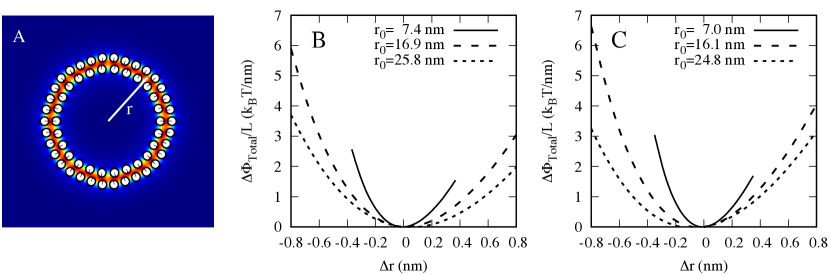
Figure 5: Panel A shows the activity field for the cross-section of a cylindrical bilayer. The radius measures from the center to the midplane. Panels B and C plot the change in energy $\displaystyle\Delta\Phi_{\mathrm{Total}}=\Phi_{\mathrm{Total}}(r)-\Phi_{\mathrm{Total}}(r_{0})$ per length of the cylinder under stretching and compression: $\displaystyle\Delta r=r-r_{0}.$ Equilibrium radius $\displaystyle r_{0}$ decreases with $\displaystyle c_{0};$ the curves are for $\displaystyle c_{0}=0.5$ pN nm⁴ in panel B, and $\displaystyle c_{0}=0.25$ pN nm⁴ in panel C ($\displaystyle\gamma=4.1$ pN nm^-1, in both panels). The solid, dashed and dotted curves use $\displaystyle N=26,$ $\displaystyle N=60$ and $\displaystyle N=92$ particles, and collapse onto a single curve when multiplied by $\displaystyle r_{0}.$

Finally, we discuss simulation data for stretching. Consider the stretching energy of a cylindrical bilayer:

(29) $$k_{\mathrm{A}}\frac{(A-A_{0})^{2}}{A_{0}},$$

where $\displaystyle A=2\pi rL,$ $\displaystyle r$ is the midplane radius, $\displaystyle L$ is the cylinder length (in the $\displaystyle z$-direction) and $\displaystyle A_{0}$ is the area at rest. The stretching modulus $\displaystyle k_{\mathrm{A}}$ is for a single monolayer and Eq. 29 accounts for the energy of the inner and outer monolayer leaflets of the cylinder. Manipulation experiments give $\displaystyle k_{\mathrm{A}}$ in the range $\displaystyle 30$ – $\displaystyle 40$ $\displaystyle\mathrm{k_{B}T}$ nm^-2 [56, 57].

To measure a stretching modulus, we form the circular cross section of cylinder of radius $\displaystyle r$ (Figure 5A). The equilibrium shape is nearly circular (so long as there is a consistent number of particles in each leaflet) and the shape obtains an equilibrium radius $\displaystyle r_{0}$ once compression and attraction are in balance. We use a harmonic bond to move $\displaystyle r$ away from equilibrium and record the change in energy (Figure 5BC).

The three curves in Figure 5B collapse onto a single curve when multplied by $\displaystyle r_{0}.$ Fitting to $\displaystyle cr_{0}(r-r_{0})^{2}$ and comparing with Eq. 29 yields $\displaystyle k_{\mathrm{A}}=33.4$ $\displaystyle\mathrm{k_{B}T}$ nm^-2, $\displaystyle 35.3$ $\displaystyle\mathrm{k_{B}T}$ nm^-2 and $\displaystyle 35.9$ $\displaystyle\mathrm{k_{B}T}$ nm^-2 for the three radii respectively. The proximity of these three values suggests that HADF possesses a stretching modulus independent of particle number. Moreover, the attraction $\displaystyle\gamma=4.1$ pN nm^-1 and repulsion parameters $\displaystyle c_{0}=0.5$ pN nm⁴ yield a consistent and physically realistic stretching modulus, around $\displaystyle k_{\mathrm{A}}=35$ $\displaystyle\mathrm{k_{B}T}$ nm${}^{-2}.$ As an illustration, the curves in Figure 5C are for the same tension parameter and half the repulsion strength. There is an overall reduction in the equilibrium radii with the decreased repulsion, and an increase in the stretching moduli $\displaystyle k_{\mathrm{A}}$ to $\displaystyle 40.310$ $\displaystyle\mathrm{k_{B}T}$ nm^-2, $\displaystyle 40.083$ $\displaystyle\mathrm{k_{B}T}$ nm^-2 and $\displaystyle 39.393$ $\displaystyle\mathrm{k_{B}T}$ nm^-2 for the three curves respectively.

HADF yields physically realistic continuum-like bilayer morphologies and these particle configurations possess elastic properties of lipid bilayer. The HADF can also handle topological changes and mixtures in a straightforward manner. Figure 6 illustrates the gradient descent dynamics of a lipid mixture between small, circular and large, elliptical particles. Under hydrophobic attraction and excluded volume repulsion, the particle mixture segregates into two bilayers of more uniform composition. Diffusive interface and level-set approaches have dealt with the problem of mixtures by defining transport equations for each lipid species density [49, 55, 25].

Hemifusion is one of the key intermediates of membrane fusion involving a Y-shaped junction between three bilayers [9](see Fig. 8, Panel C). Pioneering work by Promilsow, K. and coworkers [12, 13] has lead to functionalized Cahn-Hilliard, diffusive interface energies that exhibit freestanding elastic phases, including the Y-shaped junction [43, 21]. It is still unclear whether the HADF formulation of the present work is more or less efficient than a functionalized Cahn-Hilliard approach for capturing the granular energetic details of fusion [72].

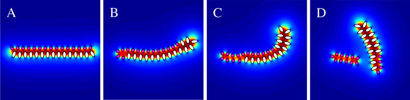
Figure 6: Panels A–D show the spontaneous sorting and eventual fission of a planar bilayer mixture of small circular particles (magenta) and elliptical particles (white). The monolayer consisting of smaller, circular particles spontaneously migrates from the bilayer edge, and eventually breaks off forming forming its own bilayer. The bending in panels B and C suggests that the smaller, circular particles have a spontaneous curvature more negative than for the larger, elliptical particles. The parameters are $\displaystyle\gamma=4.1$ pN nm^-1, $\displaystyle\rho=2.5$ nm and $\displaystyle c_{0}=0.5$ pN nm^-4 The ellipses have $\displaystyle p=6,$ $\displaystyle a_{i}=1.25$ nm and $\displaystyle b_{i}=0.6225$ nm while the circles have $\displaystyle p=2,$ $\displaystyle a_{i}=b_{i}=0.6225$ nm.

4 Hydrodynamics of amphiphilic particles in a viscous solvent

To define particle velocities, we assume that the amphiphilic particles are immersed in an incompressible viscous fluid in the Stokes flow regime. Then all the particles interact with each other through both hydrophobic forces and Stokesian hydrodynamic interactions. The two-dimensional particles $\displaystyle P_{i}$ have the translational and angular velocities

(30) $$\frac{d\mathbf{a}_{i}}{dt}=\mathbf{v}_{i},\quad\frac{d\theta_{i}}{dt}=\omega_{i},$$

$\displaystyle i=1,\dots,N.$ For the amphiphilic particles in a solvent, the forces $\displaystyle{\bf F}_{i},$ $\displaystyle{\bf F}_{i}^{\mathrm{rep}}$ and torques $\displaystyle\tau_{i},$ $\displaystyle\tau_{i}^{\mathrm{rep}}$ are calculated from Eq. 5 and Eq. 18, respectively, The velocities $\displaystyle\mathbf{v}_{i}$ and $\displaystyle\omega_{i}$ are coupled together through the fluid velocity $\displaystyle\mathbf{u}$ and pressure $\displaystyle p$ satisfying

(31) $$-\mu\Delta{\bf u}+\nabla p =0,\quad$$

$$\nabla\cdot{\bf u} =0,\quad\text{in}\ \Omega,$$

$${\bf u} \to 0\quad\text{as}\ |{\bf x}|\to\infty,$$

$$\mathbf{u}(\mathbf{x}) =\mathbf{v}_{i}+\omega_{i}(\mathbf{x}-\mathbf{a}_{i})^{\perp},\quad\mathbf{x}\in\partial P_{i},$$

with fluid viscosity $\displaystyle\mu$ and subject to the stress balance conditions

(32) $$\int_{\partial P_{i}}\mathbf{S}\cdot\mathbf{n}\,dS={\bf F}_{i}+{\bf F}_{i}^{\mathrm{rep}},\;\;\;\int_{\partial P_{i}}(\mathbf{x}-\mathbf{a}_{i})\times\mathbf{S}\cdot\mathbf{n}\,dS=\tau_{i}+\tau_{i}^{\mathrm{rep}}.$$

From Eq. 16 these particle forces and torques also satisfy the force-free and torque-free conditions, guaranteeing the existence of an integral solution for the many-body mobility problem. The evolution equations (30–32) satisfy the dissipation relation [47]

(33) $$\frac{d}{dt}\Phi_{\mathrm{Total}}+\int_{\mathbb{R}^{n}}\tfrac{1}{2}\mu|\nabla\mathbf{u}+\nabla\mathbf{u}^{T}|^{2}\,dx=0.$$

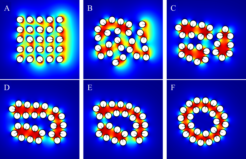
Figure 7: For large system simulations, particles self assemble into bilayer-like shapes and then eventually a cylindrical bilayer. Panels A–F are for $\displaystyle 0,$ $\displaystyle 3.8,$ $\displaystyle 19,$ $\displaystyle 76$, $\displaystyle 114$ and $\displaystyle 228$ ns, respectively; step size $\displaystyle\Delta T=1.0[T]\approx 0.38$ ns. The configuration in panel F evolves very slowly to one that is slightly more circular.

In two dimensions, the kernels of single and double layer potentials for solving the Stokes equation are the stokeslet and stresslet

(34) $$G_{i,j}^{\mathrm{Stokeslet}}({\bf x},{\bf y}) =\frac{1}{4\pi\mu}\bigg{[}\log|{\bf x}-{\bf y}|\delta_{ij}+\frac{(x_{i}-y_{i})(x_{j}-y_{j})}{|{\bf x}-{\bf y}|^{2}}\bigg{]},$$

$${\bf T}^{\mathrm{Stresslet}}_{i,j,k}({\bf x},{\bf y}) =-\frac{1}{\pi\mu}\frac{(x_{i}-y_{i})(x_{j}-y_{j})(x_{k}-y_{k})}{|{\bf x}-{\bf y}|^{4}},$$

respectively, with $\displaystyle i,j,k=1,2.$ For a velocity surface density $\displaystyle\boldsymbol{\mu},$ the stresslet satisfies the jump across the boundary

(35) $$\lim_{\mathbf{z}\rightarrow\mathbf{x}^{\pm}}\mathbf{f}_{i,\pm}(\mathbf{z})=\mp\frac{1}{2}\boldsymbol{\mu}_{i}(\mathbf{x})+\mbox{p.v.}\int_{\partial P_{i}}{\bf T}^{\mathrm{Stresslet}}_{i,j,k}({\bf x},{\bf y})\boldsymbol{\mu}_{j}(\mathbf{y})ds_{\mathbf{y}},$$

where $\displaystyle\mathbf{f}_{i}$ denotes the surface traction of on particle $\displaystyle P_{i}$. Following [67], one views the external force and torque due to hydrophobic attraction as an incident field with stress (6). The scattered field is then the net force and torque due to fluid mobility. If we split densities into $\displaystyle\boldsymbol{\sigma}^{\mathrm{inc}}({\bf x})=\{\boldsymbol{\sigma}^{\mathrm{inc}}_{1},\dots,\boldsymbol{\sigma}^{\mathrm{inc}}_{N}\}$ and $\displaystyle\boldsymbol{\mu}({\bf x})=\{\boldsymbol{\mu}_{1},\dots,\boldsymbol{\mu}_{N}\}$, then the particle dynamics  Eq. 36 can be obtained by evaluating a single layer potential for corresponding densities $\displaystyle\boldsymbol{\sigma}$ and $\displaystyle\boldsymbol{\mu}$.

(36) $${\bf u}({\bf x}) =\sum_{j=1}^{N}\int_{\partial P_{j}}G_{i,j}^{\mathrm{Stokeslet}}({\bf x},{\bf y})[\boldsymbol{\sigma}_{j}^{\mathrm{inc}}+\boldsymbol{\mu}_{j}]({\bf y})ds_{\mathbf{y}}$$

$$={\bf v}_{i}+\omega_{i}({\bf x}-{\bf a}_{i})^{\perp}\quad\forall{\bf x}\in\partial P_{i},$$

where

(37) $$\begin{split}{\bf v}_{i}&=\frac{d{\bf a}_{i}}{dt}=\frac{1}{|\partial P_{i}|}\int_{\partial P_{i}}{\bf u}({\bf y})ds_{\mathbf{y}},\quad|\partial P_{i}|=\int_{\partial P_{i}}ds_{\mathbf{y}},\\ \omega_{i}=&\tau^{-1}\int_{\partial P_{i}}({\bf y}-{\bf a}_{i})\times{\bf u}({\bf y})ds_{\mathbf{y}},\quad\tau=\int_{\partial P_{i}}|{\bf y}-{\bf a}_{i}|^{2}ds_{\mathbf{y}}.\end{split}$$

For the time-marching scheme, we solve the mobility problem for the particle translation and rotation velocities. We then update the particle centers and orientations using a forward Euler scheme. Algorithm 1 provides the time-marching details.

Non-dimensionalizing Eq. 1 with characteristic length 1.25 nm, fluid viscosity $\displaystyle\mu=1$ cP and interfacial tension $\displaystyle\gamma=4.1$ pN nm^-1 gives the characteristic time $\displaystyle[T]=\mu a/\gamma\approx 3.82\times 10^{-10}s.$ As an illustration, the evolution in Fig. 1 is for 100 time steps with time step size $\displaystyle\Delta T=1.0[T].$ The time for self assembly of a few particles from an initially random configuration is thus on the order of a nanosecond. This is consistent with times scales for lipid rearrangements in MD simulation [10]. Supplementary Materials Movie 1 shows the self-assembly process for three particles.

Bilayer configurations form when we increase the number particles in the simulation. Fig. 7A has 25 Janus-type particles placed on a square grid. The initial orientations $\displaystyle\theta_{i}$ are normally distributed about $\displaystyle\theta=0$. Within ten time steps (Fig. 7B), the particles rapidly rotate to pair their hydrophobic interfaces with that of neighboring particles. Pairings continue to merge forming groups of eight or nine particles (Fig. 7C). These groups stack together to form an arched bilayer shape resembling the cross-section of a stomatocyte (Fig. 7E). Fig. 7F clearly shows an inner and outer monolayer configuration a cylindrical bilayer.

Supplementary Materials Movie 2 illustrates the self-assembly process for Fig. 7A–F. As part of computational complexity test, we have calculated particle dynamics for larger systems and Supplementary Materials Movie 3 shows the results for 100 particles.

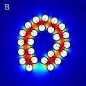
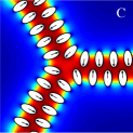
Figure 8: Panel A plots the change in energy $\displaystyle\Phi$ per length (solid curve) for the evolution Fig. 7A–F. The initial rapid decrease over 0 ns $\displaystyle<t<$ 10 ns corresponds to Fig. 7A–B. The moderate decrease over 10 ns $\displaystyle<t<$ 150 ns is for Fig. 7C–E. Energy decreases very slowly over 150 ns $\displaystyle<t<$ 600 ns, where the bilayer evolves from a somewhat elliptical cross-section (Fig. 7F) to one that is almost perfectly circular. The dashed curve gives corresponding values for a constant drag coefficient evolution: its end-state is in panel B. In panel C, the free ends of three bilayers have merged into an equilibrium, Y-shaped junction.

Is it possible to replace the detailed hydrodynamic interaction with one that uses a constant coefficient drag coefficient law? The latter also exhibits particle self-assembly and avoids the computational cost of solving an additional mobility problem. Moreover, the constant coefficient case drag laws can closely replicate the hydrodynamic interaction case when particles are dispersed (see Supplementary Material, Section S2.3). Nevertheless, numerical experiments show that the choice of dissipative mechanism is consequential to the time course. For example, Fig. 7F and Fig. 8B compare the two different end-states resulting from a identical initial configurations for a viscous fluid and for a constant drag law, respectively. The difference lies in the number of particles contained in the inner leaflet and this has determined whether or not the bilayer closes.

5 Boundary Integral Equation Formulation

In this section, we present a second kind integral equation formulation for the exterior Dirichlet problem Eq. 3. The domain $\displaystyle\Omega$ is the exterior domain, meaning that its complement $\displaystyle\Omega^{c}$ (the collection of particles) is compact.

There are a number of numerical methods for solving the exterior problem Eq. 3. These include finite difference methods, finite element methods, and boundary integral equation (BIE) methods. The BIE methods are perhaps the most suitable since they represent the solution via layer potentials with an unknown density only on the boundary. This reduces the dimension of the problem by one and leads to a much smaller linear system. Another advantage is that the integral representation automatically satisfies the governing partial differential equation and the boundary condition at infinity. Thus, there is no need to truncate the computational domain and impose artificial boundary conditions, as would be the needed with the finite element and finite difference approaches. Finally, when combined with high-order quadratures and fast algorithms such as the fast multipole methods [31, 32], the BIE formulation leads to a high-order numerical algorithm with optimal computational complexity.

Before describing the method, we first consider whether the far-field condition in Eq. 3 is sufficient to determine a unique solution. As mentioned in Section 1, the functional $\displaystyle I[\cdot]$ has a unique minimizer in $\displaystyle\mathcal{A}$. The minimizer $\displaystyle u$ satisfies $\displaystyle 0\leq u(x)\leq 1$ for all $\displaystyle x\in\Omega$. To see why these bounds holds, consider a truncated version $\displaystyle\tilde{u}=\max\{0,\min\{1,u\}\}$ of $\displaystyle u$. Because $\displaystyle 0\leq f\leq 1$ on $\displaystyle\Sigma$, $\displaystyle\tilde{u}\in\mathcal{A}$. Lastly, $\displaystyle I[\tilde{u}]\leq I[u]$ by inspection, and $\displaystyle I[u]\leq I[\tilde{u}]$ by minimality of $\displaystyle u$. This implies that $\displaystyle I[\tilde{u}]=I[u],$ and since $\displaystyle u$ is the unique minimizer, we have $\displaystyle u=\tilde{u}$.

To obtain a far-field decay condition, select a sufficiently large distance $\displaystyle D>0$ from $\displaystyle\Omega^{c}$. Let $\displaystyle x$ be such that $\displaystyle d(x,\Omega^{c})>D$. By a change of coordinates, we may assume that $\displaystyle x$ is the origin $\displaystyle(0,\dots,0)$ and that $\displaystyle\Omega^{c}$ lies in the set $\displaystyle\{(x_{1},\dots,x_{n}):x_{n}\leq-D\}$. In this coordinate system, consider the function

$$v_{\epsilon}(x_{1},\dots,x_{n})=\frac{\cosh(x_{n}/\rho)}{\cosh(D/\rho)}+\epsilon\sum_{i=1}^{n-1}\cosh(x_{i}/\rho),\quad\epsilon>0.$$

Then $\displaystyle-\rho^{2}\Delta v_{\epsilon}+v_{\epsilon}=0$ and $\displaystyle v_{\epsilon}\geq 1$ on $\displaystyle\Sigma$ (since $\displaystyle x_{n}$ is less than $\displaystyle-D$ there), and $\displaystyle v_{\epsilon}\to\infty$ as $\displaystyle|(x_{1},\dots,x_{n})|\to\infty$. Next, consider the function $\displaystyle g=v_{\epsilon}-u$. We have $\displaystyle g\geq 0$ on $\displaystyle\Sigma$ and $\displaystyle g\geq 0$ for all sufficiently large $\displaystyle(x_{1},\dots,x_{n})$ (since $\displaystyle v_{\epsilon}\to\infty$ and $\displaystyle u$ is bounded everywhere between $\displaystyle 0$ and $\displaystyle 1$).

From the weak maximum principle [26, Cor. 3.2, assuming $\displaystyle f\in C(\Sigma)$], we have $\displaystyle g\geq 0$ in $\displaystyle\Omega$. It follows that $\displaystyle v_{\epsilon}\geq u$ in $\displaystyle\Omega$. Finally, letting $\displaystyle\epsilon\to 0$, we conclude that

(38) $$0\leq u(x)\leq v_{\epsilon}(x)<2\exp(-D/\rho)$$

as soon as $\displaystyle\epsilon>0$ is sufficiently small.

The problem Eq. 3 thus has at least one solution (vanishing at infinity), namely the variational one. But since the domain $\displaystyle\Omega$ is non-compact, it is in principle possible that Eq. 3 has multiple solutions vanishing at infinity with different rates. The following Liouville-type result shows that this is not the case. In fact, we get uniqueness even if we replace the zero far-field condition with the power growth condition $\displaystyle u=O(|x|^{p})$ as $\displaystyle x\to\infty$.

Lemma 5.1.

The exterior problem Eq. 3 has at most one solution.

Proof 5.2.

Suppose that Eq. 3 has two solutions $\displaystyle u_{1}$ and $\displaystyle u_{2}$. Let $\displaystyle w=u_{1}-u_{2}$ and define

$$E(r)=\int_{\Omega\cap\mathbf{B}_{r}}\tfrac{1}{2}w^{2}\,dx,\qquad E:[0,\infty)\to[0,\infty),$$

where $\displaystyle B_{r}$ is the ball of radius $\displaystyle r$ centered at the origin. Select $\displaystyle r_{0}$ positive and sufficiently large so that $\displaystyle\Omega^{c}\subset B_{r_{0}}$.

The function $\displaystyle E(r)$ is infinitely differentiable on $\displaystyle(r_{0},\infty)$ since any solution of Eq. 3 is smooth in $\displaystyle\Omega.$ Using $\displaystyle w=0$ on $\displaystyle\Sigma$ and Eq. 3, it follows that

(39) $$E^{\prime\prime}(r)=\frac{n-1}{r}E^{\prime}(r)+\frac{1}{\rho^{2}}E(r)+\int_{\Omega\cap B_{r}}|\nabla w|^{2}\,dx,\quad r_{0}<r<\infty.$$

Since $\displaystyle E$ is nondecreasing, by definition, we get

$$E^{\prime\prime}(r)\geq\rho^{-2}E(r),\quad r_{0}<r<\infty.$$

Let $\displaystyle F(r)=\tfrac{1}{2}E(r_{0})\exp((r-r_{0})/\rho).$ We claim that

(40) $$F(r)\leq E(r),\quad r_{0}\leq r<\infty.$$

To form the comparison argument, suppose to the contrary that $\displaystyle E(r)$ is not everywhere greater than or equal to $\displaystyle F(r)$. Then $\displaystyle E(r_{0})>0$ and there is $\displaystyle r_{*}>r_{0}$ with $\displaystyle E^{\prime}(r_{*})\leq F^{\prime}(r_{*})$ and $\displaystyle F(r)<E(r)$ for $\displaystyle r_{0}\leq r<r_{*}$. But then,

$$E^{\prime}(r_{*})\leq F^{\prime}(r_{*})=\int_{r_{0}}^{r_{*}}\rho^{-2}F(r)\,dr<\int_{r_{0}}^{r_{*}}\rho^{-2}E(r)\,dr\leq E^{\prime}(r_{*})-E^{\prime}(r_{0}).$$

These inequalities are in contradiction since $\displaystyle E^{\prime}(r_{0})$ is nonnegative.

Thus, if $\displaystyle u_{1}$ and $\displaystyle u_{2}$ are two solutions of Eq. 3, then according to Eq. 40 there are one of two possibilities: either $\displaystyle E(r_{0})=0$ or one of the solutions has exponential growth. The vanishing condition $\displaystyle u\to 0$ as $\displaystyle x\to\infty$ rules out the latter case and so $\displaystyle E(r_{0})$ must be zero. Since $\displaystyle r_{0}$ was arbitrary, $\displaystyle u_{1}$ and $\displaystyle u_{2}$ are identical.

In two dimensions, the equation $\displaystyle-\rho^{2}\Delta u+u=0$ has the free-space Green’s function (also called fundamental solution)

(41) $$G(x,y)=\frac{1}{2\pi}K_{0}(|x-y|/\rho),\quad x,y\in\mathbb{R}^{2},$$

where $\displaystyle K_{0}$ is the zeroth order modified Bessel function of the first kind [62]. For a Lipschitz domain $\displaystyle\Omega$ in $\displaystyle\mathbb{R}^{2}$ with boundary $\displaystyle\Sigma$, the space $\displaystyle L^{2}(\Sigma)$ denotes all square integrable functions on $\displaystyle\Sigma$. Given a function $\displaystyle\sigma\in L^{2}(\Sigma)$, we define the single layer potential by the formula

(42) $$\mathcal{S}[\sigma](x)=\int_{\Sigma}G(x,y)\sigma(y)ds_{y},$$

and the double layer potential by the formula

(43) $$\mathcal{D}[\sigma](x)=\int_{\Sigma}\frac{\partial G(x,y)}{\partial\nu(y)}\sigma(y)ds_{y},$$

where $\displaystyle\nu(y)$ is the unit outward normal vector with respect to $\displaystyle\Omega^{c}$. It is well-known from classical potential theory [44] that the single layer potential is continuous and the double layer potential exhibits a jump across the boundary. To be more precise, when $\displaystyle z$ approaches a point $\displaystyle x\in\Sigma$ nontangentially, the limits of $\displaystyle\mathcal{S}[\sigma]$ and $\displaystyle\mathcal{D}[\sigma]$ exist and are given by the following formulas:

(44) $$\lim_{z\rightarrow x^{\pm}}\mathcal{S}[\sigma](z)=S[\sigma](x)=\int_{\Sigma}G(x,y)\sigma(y)ds_{y},$$

and

(45) $$\lim_{z\rightarrow x^{\pm}}\mathcal{D}[\sigma](z)=(\pm\frac{1}{2}I+D)[\sigma](x)=\pm\frac{1}{2}\sigma(x)+\mbox{p.v.}\int_{\Sigma}\frac{\partial G(x,y)}{\partial\nu(y)}\sigma(y)ds_{y},$$

for almost every point $\displaystyle x\in\Sigma$. Here $\displaystyle z\rightarrow x^{\pm}$ implies that $\displaystyle z$ approaches $\displaystyle x$ from the exterior$\displaystyle(+)$ or the interior$\displaystyle(-)$ of $\displaystyle\Omega^{c}$, respectively. It is also well-known that both the single layer operator $\displaystyle S:L^{2}(\Sigma)\rightarrow L^{2}(\Sigma)$ and the double layer operator $\displaystyle D:L^{2}(\Sigma)\rightarrow L^{2}(\Sigma)$ are compact when the boundary $\displaystyle\Sigma$ is $\displaystyle C^{1}$.

We will represent the solution to Eq. 3 with the double layer potential representation:

(46) $$u(x)=\mathcal{D}[\sigma](x).$$

The jump relation of the double layer potential Eq. 45 leads to the following boundary integral equation on the unknown density $\displaystyle\sigma$:

(47) $$\frac{1}{2}\sigma(x)+D[\sigma](x)=f(x),\quad x\in\Sigma.$$

Algorithm 1 Particle Updates by Exterior Screened Laplace BVP

1:  Set the particle centers $\displaystyle\mathbf{a}_{i}\in\mathbb{R}^{2}$ and orientations $\displaystyle\theta_{i}\in\mathbb{R}$, boundary condition $\displaystyle f(x)$ and time step size $\displaystyle\Delta t$

2:  Determine the discretization on the boundary $\displaystyle\Sigma$ and construct the double layer potential $\displaystyle\mathcal{D}[\sigma](x)$.

3:  for $\displaystyle t=t_{0}:t_{end}$ do

4:     Use GMRES iterative method to solve the unknown density $\displaystyle\sigma$ in Eq. 47.

5:     Use the solved $\displaystyle\sigma$ to obtain the screend Laplace equation solution $\displaystyle u$ and calculate $\displaystyle\nabla u$.

6:     Calculate inter-molecular forcesr Eq. 5 and Eq. 19.

7:     Use GMRES iterative method to solve the unknown density $\displaystyle\boldsymbol{\mu}$ in Eq. 35.

8:     Solve mobility problemand update particle velocities $\displaystyle{\bf v}_{i}$ and $\displaystyle\omega_{i}$ in Eq. 36.

9:     Update particle center positions $\displaystyle{\bf a}_{i}$ and orientations $\displaystyle\theta_{i}$.

10:     Update the marching time $\displaystyle t=t_{0}+\Delta t$.

11:  end for

12:  return  $\displaystyle T$

Theorem 5.3.

Suppose that $\displaystyle\rho$ is any positive real number. Then for any $\displaystyle f\in L^{2}(\Sigma)$, the second kind integral equation Eq. 47 is uniquely solvable.

Proof 5.4.

By the Fredholm alternative [44], we only need to show that the only solution to the homogeneous equation

(48) $$\frac{1}{2}\sigma(x)+D[\sigma](x)=0.$$

is $\displaystyle\sigma\equiv 0$.

Consider the function $\displaystyle u(x)$ defined by the formula Eq. 46. It is clear that $\displaystyle u$ satisfies the equation $\displaystyle-\rho^{2}\Delta u+u=0$ in both the exterior domain $\displaystyle\Omega$ and the interior domain $\displaystyle\Omega^{c},$ and vanishes at infinity. By the uniqueness of the exterior Dirichlet problem (Lemma 5.1), we have $\displaystyle u\equiv 0$ in $\displaystyle\Omega$. Hence,

(49) $$\lim_{z\rightarrow x^{+}}\frac{\partial u(z)}{\partial\nu}=0,\quad x\in\Sigma.$$

Since the normal derivative of the double layer potential is continuous across the boundary [44, gen. of Thm. 6.18], we have

(50) $$\lim_{z\rightarrow x^{-}}\frac{\partial u(z)}{\partial\nu}=0,\quad x\in\Sigma.$$

Hence, $\displaystyle u$ in the interior domain $\displaystyle\Omega^{c}$ is the solution to the interior Neumann problem

(51) $$-\rho^{2}\Delta u+u=0,\quad u\in\Omega^{c},\quad\frac{\partial u}{\partial\nu}=0,\quad x\in\Sigma.$$

Applying Green’s first identity, we obtain

(52) $$\int_{\Omega^{c}}\rho^{2}|\nabla u|^{2}+u^{2}dx=0.$$

Thus we have $\displaystyle u\equiv 0$ in $\displaystyle\Omega^{c}$ as well. The jump relation of the double layer potential Eq. 45 leads to

(53) $$\sigma(x)=\lim_{z\rightarrow x^{+}}u(z)-\lim_{z\rightarrow x^{-}}u(z)=0,\quad x\in\Sigma,$$

which completes the proof.

Remark 5.5.

As pointed out earlier, the screened Laplace equation can be viewed as the Helmholtz equation $\displaystyle\Delta u+k^{2}u=0$ with pure imaginary $\displaystyle k$. When $\displaystyle k$ is an arbitrary complex number, the so-called Brakhage-Werner representation [5] (also called the Burton-Miller representation [7] in acoustics) represents the solution to the Helmholtz equation via a linear combination of single and double layer potentials

(54) $$u(x)=i\mathcal{S}[\sigma](x)+\mathcal{D}[\sigma](x).$$

It has been shown that the representation Eq. 54 leads to a uniquely solvable second kind integral equation for any value of $\displaystyle k\in\mathbb{C}$ [59]. Due to the exponential decay of the solution to our exterior problem Eq. 3, we are able to use the double layer potential alone to represent its solution and still achieve existence and uniqueness of the associated boundary integral equation Eq. 47.

We would like to point out that when $\displaystyle\rho$ is very large, the formulation Eq. 54 may lead to a better conditioned linear system than Eq. 46. There are other second kind integral equation formulations for this problem. For example, one may replace the single layer potential by a collection of point sources inside each particle, where the strength of the point source may be unknown or equal to the average value of the unknown density function on the boundary of each particle. We refer the readers to [29, 30, 36] for details.

6 High-order quadrature and fast algorithms

Figure 9: Geometric situation of a single QBX expansion with sources along the collection of curves $\displaystyle\Sigma$, as used in Eq. 55 and Eq. 56. Note that the target point $\displaystyle x$ will reside on $\displaystyle\Sigma$ for the computation of the on-surface value of the layer potential.

For the accurate and rapid evaluation of the layer potentials occurring in the previous section, we make use of ‘Quadrature by Expansion’, or QBX for short [39]. Here we briefly review the QBX scheme for the general Helmholtz kernel and note that the Yukawa kernel Eq. 41 is simply a special case of the Helmholtz kernel with pure imaginary wave number $\displaystyle k$. To do so, we cover a neighborhood of the source curve $\displaystyle\Sigma$ with locally valid (‘local’) expansions of the potential emanating from the entire source curve $\displaystyle\Sigma$. For a collection of on-surface target points $\displaystyle(x_{i})$, expansion centers are chosen as $\displaystyle c_{i}=x_{i}+\nu\eta_{x_{i}}$, where $\displaystyle\eta_{x}$ is a scaling factor connected to the local quadrature resolution. See [79] for details of the determination of $\displaystyle\eta_{x}$. Then, for target points $\displaystyle x\in B(c_{i},\eta_{x_{i}})$, the layer potential may be evaluated as

(55) $$\phi(x)=\sum_{l=-\infty}^{\infty}\alpha_{l}J_{l}(k\rho)e^{-il\theta}$$

where $\displaystyle(\rho,\theta)$ denote the polar coordinates of the target point $\displaystyle x$ with respect to the expansion center $\displaystyle c$, and $\displaystyle J_{l}$ is the Bessel function of order $\displaystyle l$ (see Fig. 9). For the single layer potential $\displaystyle S\sigma$, the coefficients $\displaystyle\alpha_{l}$ in the expansion (55) can be computed analytically:

(56) $$\alpha_{l}=\frac{i}{4}\,\int_{\Sigma}H^{(1)}_{l}(k|x^{*}-c|)e^{il\theta^{*}}\sigma(x^{*})dx^{*},\qquad(l=-p,-p+1,\ldots,p)$$

where $\displaystyle(|x^{*}-c|,\theta^{*})$ denote the polar coordinates of the point $\displaystyle x^{*}$ with respect to $\displaystyle c$. These (now non-singular) integrals for the coefficients $\displaystyle\alpha_{l}$ are then computed by conventional high-order numerical quadrature. These formulas follow immediately from Graf’s addition theorem [62, (10.23.7)],

(57) $$H^{(1)}_{0}(k|x-x^{*}|)=\sum_{l=-\infty}^{\infty}H^{(1)}_{l}(k|x^{*}-c|)e^{il\theta^{*}}J_{l}(k|x-c|)e^{-il\theta},$$

This identity applies directly to the Yukawa potentials under consideration here, based on the fact that $\displaystyle K_{0}(z)=(i\pi/2)H_{0}^{(1)}(iz)$, cf. [62, (10.27.8)]. Separation-of-variables results similar to Graf’s addition theorem hold for Laplace potentials, allowing us to proceed analogously in that case [31]. The QBX procedure described above employs two means of approximation: the truncation of the series expansion, and the computation of the coefficients by numerical quadrature. We give an error result for QBX that accounts for both aspects. For the following result, we consider the case of the double layer and assume $\displaystyle c=0$ without loss of generality.

Theorem 6.1 (QBX truncation and quadrature errors, [16, Thm. 2.5 and (4.6)]).

Suppose that $\displaystyle\Gamma$ is a smooth, bounded curve embedded in $\displaystyle\mathbb{R}^{2}$, such that $\displaystyle B_{\eta_{x}}(0)\cap\Gamma=\emptyset$, but $\displaystyle\rho e^{i\theta}\in\overline{B}_{\eta_{x}}(0)\cap\Gamma$. Assume the geometry $\displaystyle\Gamma$ is discretized using $\displaystyle q$ point composite Gauss-Legendre panels of uniform length $\displaystyle h$, with a total of $\displaystyle n$ points.

For $\displaystyle k\in[0,\infty)$, $\displaystyle N$ a positive integer, and $\displaystyle\beta>0$, there are constants $\displaystyle C^{\prime}_{N,\beta,\Gamma}(k)$ and $\displaystyle C^{\prime\prime}_{q,\Gamma}(k)$, so that if $\displaystyle\sigma\in C^{N,\beta}(\Gamma)$, then

(58) $$\left|\lim_{r\to\rho^{-}}\int_{\Gamma}\frac{\partial G(re^{i\theta},y)}{\partial\nu(y)}\sigma(y)ds(y)-\sum_{l=1-N}^{N-1}Q_{q}(\alpha_{l})J_{l}(k\rho)e^{-il\theta}\right|\\ \leq C^{\prime}_{N,\beta,\Gamma}(k)\rho^{N}\|\sigma\|_{C^{N,\beta}(\Gamma)}+C^{\prime\prime}_{q,\Gamma}(k)\frac{h^{2q}}{{(4r)}^{2q+1}}\|\sigma\|_{C^{2q}}.$$

Here the coefficients $\displaystyle\{\alpha_{l}\}$ are given by Eq. 56, and $\displaystyle Q_{q}(\alpha_{l})$ denotes the approximation of the coefficient integral of Eq. 56 by Gaussian quadrature with $\displaystyle q$ points.

The theorem makes several assumptions that may not be true of the geometry discretization in its original form, notably the assumption that the placed disks do not intersect with other geometry, or the requirement that source panels supply sufficient quadrature resolution not just for themselves, but also for adjacent panels (which masquerades in Theorem 6.1 as the assumption of equal panel sizes). All these issues can be remedied by adequate refinement of the source geometry. An efficient, tree-based algorithm is available [79] to accomplish this.

To avoid quadratic scaling of the computational cost with the number of degrees of freedom, boundary integral equation methods require some form of acceleration, often through a variant of the Fast Multipole method (FMM [8]). In the context of QBX, it is convenient to exploit that the expansions produced as the output of the far-field stage of the FMM are the same ones employed by the quadrature method. However, without some care, loss of accuracy may occur [68]. We make use of the ‘GIGAQBX’ fast algorithm of [80] to obtain guaranteed accuracy at linearly scaling cost. This algorithm modifies the conventional FMM by forcing direct computation of interactions that may endanger the accuracy of the computed QBX expansion, in addition to a number of modifications to retain efficiency and linear scaling in that setting.

Another feature in GIGAQBX is the adaptive refinement activated when two or more source geometries get close to each other, causing near-singular evaluations of the boundary integral. The adaptive refinement is designed to continue until the expansion disks get out of the region of the source geometry [80]. Under the HADF, one might expect that many levels of refinement are needed when two particles are brought to near contact. However, the steric potential Eq. 19 also acts to prevent particles from getting too close to each other.

With the use of the short range repulsive potential, we found that the count of continuous refinements to be at most 3 to 5 levels at each time step for simulations presented in this work. Moreover, if the target point is geometrically on the wrong side (e.g. the interior region for the exterior problem), the GIGAQBX approximates analytic continuation of the potential across the boundary $\displaystyle\Gamma$, leading to benign behavior even in degenerate cases.

Our simulation codes make use of the software package ‘Pytential’ [40], which is in turn built upon FMMlib [27] for some of its expansion and translation operator infrastructure.

7 Conclusions

Topological transitions of a lipid bilayer membrane, such as membrane fusion and fission, involve rearrangement of lipid molecules in the bilayer. Consequently the well-known Helfrich free energy requires modification to account for lipid granularity to resolve the detailed lipid re-modeling during membrane fusion or fission [61, 13, 72]. By using a modified Helfrich free energy with van der Waals repulsion and a hydrophobic potential for lipid tail-solvent interaction, Ryham et al. [72] calculated a least energy pathway of membrane fusion. Building on these results, the main motivation for the work presented here is to construct a hybrid continuum lipid model at the mesoscopic scales to capture both the lipid granularity and the long-range interaction during the self-assembly of lipid molecules and fusion/fission dynamics of a lipid bilayer membrane.

Our continuum coarse-grained model for lipids focuses on the hydrophobic interactions between lipid tails, and an SKIE formulation of the hydrophobic stress is derived and used for obtaining particle dynamics. We also show that the long-range hydrophobic attraction potential is non-pairwise, and thus requires special treatment within the coarse-grained model framework. The GIGAQBX scheme—an improved version of the QBX-FMM scheme with guaranteed accuracy—is used in the discretization, solver, and evaluation phases of the SKIE to achieve high accuracy and asymptotically optimal complexity. Simulation results of our model show that during the self-assembly process, coarse-grained lipid particles form structures (such as micelles and bilayers) that may further fuse together to form a single bilayer membrane. These results show that our approach can naturally capture the mesoscopic dynamics of membrane fusion/fission. Furthermore, we show that the hydrophobic interactions give rise to membrane curvature minimization, which is an indication of the origin of bending rigidity in a bilayer membrane.

It is straightforward to apply the numerical scheme developed in this paper to study particles of arbitrary shape. With slight algorithmic modification, the scheme can also accurately capture the collision dynamics that many researchers may regard as rather difficult to deal with.

We also illustrate that the lipid hydrodynamics under HADF gives rise to macroscopic mechanical properties of a lipid bilayer membrane that are consistent with other results in the literature. The flexibility of our hybrid approach allows us to consider a mixture of two lipid species and how spontaneous sorting (phase separation) of two lipid species leads to membrane fission, consistent with results from phase-field simulations [49]. Our future goal is to extend the current framework to three-dimensional lipid system. We will incorporate fluctuating hydrodynamics into the boundary integral formulation to extract physical properties of the lipid bilayer membrane such as membrane diffusivity, bending rigidity and the surface tension. By modification of the interfacial labels, HADF can account for charged lipids and study their impact on elastic properties of bilayer [20]. Since we have immersed the particles in a zero-Reynolds flow, it is possible to study the rheological properties of micelle networks in large particle simulations [50]. Finally, we also aim to investigate the continuum limit of our hybrid model and make comparison with functionalized Canham-Helfrich models.

Appendix A Pairwise potentials

We show that pairwise potentials do not closely approximate the HADF. Consider the case of $\displaystyle N$ many particles in general position and orientation. Their associated pairwise potential is

(59) $$\sum_{i=1}^{N}\sum_{j>i}\phi_{ij},$$

where $\displaystyle\phi_{ij}$ is the functional (1) evaluated on $\displaystyle\Omega=\mathbb{R}^{2}\setminus(P_{i}\cup P_{j}).$ Differentiating Eq. 59 with respect to position $\displaystyle\mathbf{a}_{i}$ yields the force

(60) $$\mathbf{f}_{i}=\sum_{j\neq i}\mathbf{f}_{ij},\quad\mathbf{f}_{ij}=-\nabla_{\mathbf{a}_{i}}\phi_{ij}.$$

That is, we calculate $\displaystyle\mathbf{f}_{ij}$ using Eq. 5 for a fluid domain containing only two particles, $\displaystyle P_{i}$ and $\displaystyle P_{j},$ and then sum the results for $\displaystyle j=1,\dots,N,$ $\displaystyle j\neq i.$ Finally, let $\displaystyle\Phi$ be the HADF for all $\displaystyle N$ particles, and calculate the hydrophobic force $\displaystyle\mathbf{F}_{i}=-\nabla_{\mathbf{a}_{i}}\Phi$ using Eq. 5 over the fluid domain that contains all particles.

The table in Figure 10 compares the non-pairwise $\displaystyle\mathbf{F}_{i}$ and pairwise $\displaystyle\mathbf{f}_{i}$ forces for a sample particle configuration (Figure 10, pseudo-color map). The forces show significant differences for all six particles (Figure 10, rightmost column), suggesting that it is insufficient to use a pairwise potential to calculate HADF as formulated in the present work. We note, however, that owing to the form of the free-space Green’s function Eq. 41, the correlations between particles decays like $\displaystyle\exp(-D/\rho)$ in their distance $\displaystyle D.$ This makes it possible localize interaction to tens of particles by setting a cut-off radius in the layer potential evaluations.

Supplementary Material: Amphiphilic InteractionS.-P. P. Fu, R. J. Ryham, A. Klöckner, M. Wala, S. Jiang, and Y.-N. Young

Supplementary Material

Simulation of Multiscale Hydrophobic Lipid Dynamics via Efficient Integral Equation Methods

Szu-Pei P. Fu${}^{1,*},$ Rolf J. Ryham${}^{1},$ Andreas Klöckner${}^{2},$ Matt Wala${}^{2},$ Shidong Jiang${}^{3},$, Y.-N. Young${}^{3},$

¹Fordham University, Department of Mathematics, Bronx, NY, USA

²Department of Computer Science, University of Illinois at Urbana-Champaign, Urbana, IL 61801 USA

³Department of Mathematical Sciences, New Jersey Institute of Technology, Newark, NJ 07102 USA

^∗Corresponding author. Address: Fordham University, Department of Mathematics, 441 E. Fordham Rd, Bronx, NY 10458. email: sfu17@fordham.edu

Appendix S1 Elliptical Excluded Volume Repulsion

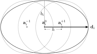
Figure S1: Schematic of elliptical repulsion.

For any elliptical particle with semi-major axis $\displaystyle a_{i}$ and semi-minor axis $\displaystyle b_{i}$, the rigid body repulsion is designed as follows. Consider three circle centers $\displaystyle\mathbf{a}_{i}^{k}=\mathbf{a}_{i}+kh\mathbf{d}_{i},$ $\displaystyle h=(a_{i}-b_{i}),k\in\{-1,0,+1\}$ with radii $\displaystyle b_{i}$ (Figure S1) and use Eq. 19 with $\displaystyle c_{0}$ divided by 3 to calculate the forces $\displaystyle\mathbf{f}^{k}_{i},k\in\{-1,0,+1\}$ and torque $\displaystyle\tau_{i}^{-1}$ and $\displaystyle\tau_{i}^{+1}$. For two elliptical particles, the total interactions are given by

(S1) $$\begin{gathered}\mathbf{f}^{kl}_{ij}=\frac{c_{0}}{3}\frac{q}{(|\mathbf{a}_{i}^{k}-\mathbf{a}_{j}^{l}|-(b_{i}+b_{j}))^{q+1}}\frac{\mathbf{a}_{i}^{k}-\mathbf{a}_{j}^{l}}{|\mathbf{a}_{i}^{k}-\mathbf{a}_{j}^{l}|},\quad i\neq j,\quad k,l\in\{-1,0,+1\},\\ \mathbf{F}^{\mathrm{rep}}_{i}=\sum_{\begin{subarray}{c}j=1\\ j\neq i\end{subarray}}^{N}\sum_{k,l}\mathbf{f}^{kl}_{ij},\quad k,l\in\{-1,0,+1\},\\ \tau_{i}^{\mathrm{rep}}=\sum_{\begin{subarray}{c}j=1\\ j\neq i\end{subarray}}^{N}\sum_{k}h(\mathbf{f}^{-1k}_{ij}-\mathbf{f}^{+1k}_{ij})\times\mathbf{d}_{i},\quad k\in\{-1,0,+1\}.\end{gathered}$$

The total repulsive potential is

(S2) $$\Phi_{i}^{\mathrm{rep}}=\frac{1}{2}\sum_{\begin{subarray}{c}j=1\\ j\neq i\end{subarray}}^{N}\sum_{k}\frac{c_{0}}{3}\frac{1}{(|\mathbf{a}_{i}^{k}-\mathbf{a}_{j}^{l}|-(b_{i}+b_{j}))^{q}},\quad k\in\{-1,0,+1\}.$$

The total repulsive force is identical to Eq. 19 whenever particles are circular.

Appendix S2 Numerical Validations

S2.1 Force and Torque Relations

We validate formulas (5, 6) by centered difference approximation. Following Eq. 13,

(S3) $$\mathbf{v}\cdot\mathbf{F}_{i} =-\frac{d}{d\epsilon}\Phi(\mathbf{a}_{i}+\epsilon\mathbf{v},\theta_{i})|_{\epsilon=0}\approx-\frac{\Phi(\mathbf{a}_{i}+\epsilon\mathbf{v},\theta_{i})-\Phi(\mathbf{a}_{i}-\epsilon\mathbf{v},\theta_{i})}{2\epsilon},$$

$$\omega\tau_{i} =-\frac{d}{d\epsilon}\Phi(\mathbf{a}_{i},\theta_{i}+\omega\epsilon)|_{\epsilon=0}\approx-\frac{\Phi(\mathbf{a}_{i},\theta_{i}+\omega\epsilon)-\Phi(\mathbf{a}_{i},\theta_{i}-\omega\epsilon)}{2\epsilon},$$

where $\displaystyle i=1,\dots,N$. We write $\displaystyle\Phi(\mathbf{a}_{i},\theta_{i})$ in place of $\displaystyle\Phi(\Omega,f)$ to emphasize that for the moment variations are taken with respect to the $\displaystyle i$th particle, while keeping the others particles fixed. For the three-particle setup from Fig. 1A and step size $\displaystyle\epsilon=0.05,$ we get the following values:

Centered Difference	Variations (5-6)
$\displaystyle\mathbf{F}_{i}$ $\displaystyle\tau_{i}$ $\displaystyle\langle-0.94496,+1.37954\rangle$ $\displaystyle+0.90685$ $\displaystyle\langle-0.28603,-0.46196\rangle$ $\displaystyle+0.02815$ $\displaystyle\langle+1.17189,-0.90103\rangle$ $\displaystyle-0.23972$	$\displaystyle\mathbf{F}_{i}$ $\displaystyle\tau_{i}$ $\displaystyle\langle-0.83884,+1.35038\rangle$ $\displaystyle+0.92534$ $\displaystyle\langle-0.26879,-0.43257\rangle$ $\displaystyle+0.02923$ $\displaystyle\langle+1.20538,-0.91928\rangle$ $\displaystyle-0.23962$

The agreement between the centered difference approximation and the variational derivatives supports (5-6).

S2.2 Single Particle Validation

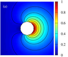
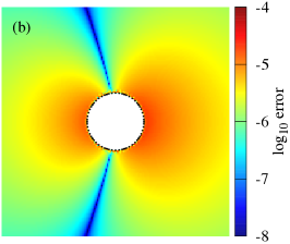
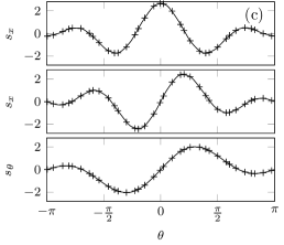
Figure S2: Single Janus particle simulation ($\displaystyle\rho=4a$): (a) Surface-contour plot of the action field solution $\displaystyle u.$ The points along the boundary (circle) show the distribution of panels and Gauss-Legendre points. (b) Error plot (in logarithmic scale) for the BIE-QBX-FMM solution and analytical solution S4. (c) From top to bottom: normal and tangential stresses calculated by BIE-QBX-FMM (+ symbols) and their corresponding analytical values (solid curves).

One can analytically solve the exterior problem Eq. 3 for a single two-dimensional disk with boundary condition Eq. 17 using the free-space Green’s function Eq. 41;

(S4) $$u(r,\theta)=\frac{1}{2}\left(\frac{K_{0}\left(\frac{r}{\rho}\right)}{K_{0}\left(\frac{a}{\rho}\right)}+\frac{K_{1}\left(\frac{r}{\rho}\right)}{K_{1}\left(\frac{a}{\rho}\right)}\cos\left(\theta\right)\right).$$

Here $\displaystyle(r,\theta)$ are polar coordinates relative to the particle center (the origin), $\displaystyle\mathbf{d}_{1}=\langle 1,0\rangle$ is the particle orientation, and $\displaystyle a$ and $\displaystyle\rho=4a$ are the disk radius and decay length, respectively.

Figure S2(a) shows of the action field contours for Eq. S4. Consistent with the boundary condition Eq. 17, the hydrophobic attraction is strongest in the neighborhood of the right semicircle. The smooth boundary data results in the hydrophobic attraction extending weakly to the left of the particle. The size of the contours are proportional to the decay length $\displaystyle\rho$, e.g. the farthest contour $\displaystyle u(r,\theta)=0.1$ in Figure S2(a) would grow for larger $\displaystyle\rho$.

Figure S2(b) shows the corresponding relative errors of the BIE-QBX-FMM with $\displaystyle N_{\rm bdy}=70$ boundary points and QBX order $\displaystyle p=6$. The reflectional symmetry of the error distribution is due to the symmetric particle shape and boundary condition. The numerically computed interfacial stresses (e.g. gradients in the action field) are also in excellent agreement with their analytical values. In Figure S2(c), the + markers are for the numerically calculated pointwise normal and tangential stress densities,

(S5) $$\langle s_{x}(\theta),s_{y}(\theta)\rangle=\mathbf{T}(a,\theta)\cdot\mathbf{i}_{r},\quad s_{\theta}(\theta)=\mathbf{i}_{r}\times(\mathbf{T}(a,\theta)\cdot\mathbf{i}_{r}),$$

respectively, along the particle boundary. The smooth curves Figure S2(c) are the analytical values, obtained by plugging Eq. S4 into the integrands of the equations Eq. 12. Thus the BIE-QBX-FMM yields a numerical solution that is highly accurate both in terms of the action field and its gradients along the domain boundary. From a physical perspective, an isolated particle has zero net force and torque (see Eq. 16). Indeed, the integrals of force and torque curves in Figure S2(c) are all zero to about eight digit accuracy.

Table 1: Convergence tests as the QBX order $\displaystyle p$ and number panels per particle $\displaystyle N_{\rm pan}$ vary. The number of Gauss-Legendre points $\displaystyle N_{\rm GL}=6$ per panel (yielding $\displaystyle N_{\rm bdy}=N_{\rm GL}N_{\rm pan}$ points per particle), FMM order $\displaystyle p_{FMM}=10,$ GMRES tolerance $\displaystyle tol_{\rm GMRES}=10^{-13}$ and $\displaystyle 5\times 5$ computational domain are fixed. $\displaystyle N_{\rm iter}$ is the number of iterations in GMRES.

$\displaystyle N_{\rm pan}$ 10 20 40 80

$\displaystyle N_{\rm bdy}$ 70 140 280 560

QBX order $\displaystyle p=4$ $\displaystyle N_{\rm iter}$ $\displaystyle l_{\infty}$ error $\displaystyle 8$ $\displaystyle 3.20\times 10^{-4}$ $\displaystyle 8$ $\displaystyle 2.00\times 10^{-5}$ $\displaystyle 7$ $\displaystyle 9.12\times 10^{-7}$ $\displaystyle 8$ $\displaystyle 5.96\times 10^{-8}$

QBX order $\displaystyle p=6$ $\displaystyle N_{\rm iter}$ $\displaystyle l_{\infty}$ error $\displaystyle 8$ $\displaystyle 2.01\times 10^{-5}$ $\displaystyle 7$ $\displaystyle 3.93\times 10^{-7}$ $\displaystyle 8$ $\displaystyle 2.21\times 10^{-7}$ $\displaystyle 9$ $\displaystyle 4.77\times 10^{-8}$

QBX order $\displaystyle p=8$ $\displaystyle N_{\rm iter}$ $\displaystyle l_{\infty}$ error $\displaystyle 8$ $\displaystyle 1.23\times 10^{-6}$ $\displaystyle 7$ $\displaystyle 1.23\times 10^{-8}$ $\displaystyle 8$ $\displaystyle 2.84\times 10^{-7}$ $\displaystyle 8$ $\displaystyle 5.01\times 10^{-8}$

Continuing with the single particle test, Table 1 provides three sets of convergence tests where we tune the QBX parameters. The purpose of these tests is to acquire a suitable parameter set for efficient simulations. We fix the GMRES iterative scheme tolerance $\displaystyle tol_{\rm GMRES}=10^{-13}$ and use the FMM to expedite the matrix-vector multiplications in GMRES iterations. We divide each particle boundary into $\displaystyle N_{\rm pan}$ panels and fill in $\displaystyle N_{\rm GL}$ Gauss-Legendre points in each panel. This yields a total number of boundary points $\displaystyle N_{\rm bdy}=N_{\rm GL}N_{\rm pan}$. In the $\displaystyle l_{\infty}$ error columns, we compute the errors with respect to the analytical solution Eq. S4 over a 5 $\displaystyle\times$ 5 computational domain sampling at 200 $\displaystyle\times$ 200 cartesian grid points (the error excludes the values inside the particle). Through our setting of the underlying fast multipole order $\displaystyle p_{FMM}=10$, the approximation of the layer potential has about eight digit accuracy, leading to the observed errors ‘bottoming out’ around that accuracy. As a result, the results for order $\displaystyle p=10$ are only marginally better than for the $\displaystyle p=8$ column, but require significantly more computational time.

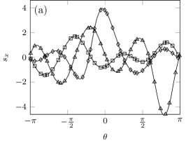
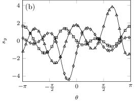
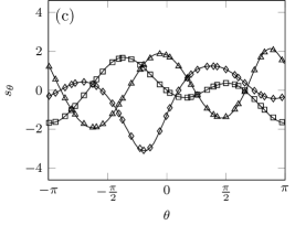
Figure S3: Panels (a) and (b) show the normal stresses $\displaystyle s_{x}$ and $\displaystyle s_{y},$ and panel (c) is for the tangential stress $\displaystyle s_{\theta}$ S5. The symbols are: $\displaystyle\diamond$-diamond for particle 1, $\displaystyle\square$-square for particle 2 and $\displaystyle\triangle$-triangle for particle 3. Net force and torque is zero 16 and so the integrals of the curves in panel (a) sum to zero. The same holds for panel (b) and for panel (c).

S2.3 Dissipative System with Constant Drag Coefficients

As an alternative numerical scheme, the metastable final states of self-assembly particles are achievable by using constant drag coefficients to update particle dynamics. The updated particle dynamics of centers $\displaystyle\mathbf{a}_{i}\in\mathbb{R}^{2}$ and orientations $\displaystyle\theta_{i}\in\mathbb{R}$ at $\displaystyle t=n\Delta t$ are given by

(S6) $${\bf a}_{i}^{n+1}={\bf a}_{i}^{n}+\frac{1}{\xi_{x}}\bigg{(}\mathbf{F}_{i}+\sum_{j\neq i}\mathbf{F}_{ij}^{\mathrm{rep}}\bigg{)}\Delta t,\quad\theta_{i}^{n+1}=\theta_{i}^{n}+\frac{1}{\xi_{\theta}}\tau_{i}\Delta t.$$

To discretize Eq. S6, we adopt the forward Euler scheme for configuration updates. We observe numerically, and use the values $\displaystyle\xi_{\bf x}=4\pi\mu a$ and $\displaystyle\xi_{\theta}=4\pi\mu a^{3}$ for an isolated circular particle of radius $\displaystyle a$ and $\displaystyle\mu=1\$cP for water viscosity. The numerical scheme for simulating dissipative system using proposed constant drag law is included in Algorithm 1.

This numerical test is to investigate a rough approximation of constant drag coefficients $\displaystyle\xi_{\bf x}$ and $\displaystyle\xi_{\theta}$. We first place two circular particles on the same horizontal axis, with centers $\displaystyle\mathbf{a}_{1}=\langle-2.5,0\rangle$ and $\displaystyle\mathbf{a}_{2}=\langle 2.5,0\rangle$, and orientations $\displaystyle\theta_{1}=45^{\circ}$ and $\displaystyle\theta_{2}=135^{\circ}$ (The schematic is in Figure S4A). From the theory of HADF, the particle pair will move toward each other and rotate until the system energy reaches a minimum. Due to the effect of excluded volume repulsion, with the choice of $\displaystyle c_{0}=0.0166$ pN nm⁴, an equilibrium distance $\displaystyle r_{12}$ between two particles can be measured. Three sets of simulations are performed: (1) Obtaining particle dynamics by solving a mobility problem; (2) Calculating dissipative dynamics using three dimensional translational and rotational drag coefficients $\displaystyle\xi_{\bf x}=6\pi\eta a$ and $\displaystyle\xi_{\bf x}=8\pi\eta a^{3}$ and (3) Calculating dissipative dynamics using translational and rotational drag coefficients $\displaystyle\xi_{\bf x}=4\pi\eta a$ and $\displaystyle\xi_{\bf x}=4\pi\eta a^{3}$. Both Figure S4B and Figure S4C show that the dynamics obtained from case (2) have much lower initiative translational and rotational velocity. Case (3) gives a very good agreement in dynamics for the first few nanoseconds. To explain this finding, from Stokesian dynamics, the resistance tensor is a function of particle pair-distances and the particle resistance will be a factor of $\displaystyle\log(r_{ij})$ in two dimensions. This observation shows that with a specific choice of constant drag coefficients the dynamics of many-body system may have very similar starting transition in self-assembly.

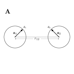
Figure S4: Panel A: Schematic of two-particle simulations; Panel B: Plot of particle 2 orientations over time in three cases; Panel C: Plot of distance $\displaystyle r_{12}$ over time in three cases.

S2.4 Multiple Particle Cases

For three-particle dynamics, there is no closed-form solution to compare with, and so we use a piecewise linear FEM to perform the numerical validations. The three particle configuration is the same as in 1(a), with centers $\displaystyle\mathbf{a}_{1}=\langle-1,0\rangle,$ $\displaystyle\mathbf{a}_{2}=\langle 1.5,3.3\rangle$ and $\displaystyle\mathbf{a}_{3}=\langle 1.5,-1.5\rangle,$ and orientations $\displaystyle\theta_{1}=18^{\circ},$ $\displaystyle\theta_{2}=240^{\circ}$ and $\displaystyle\theta_{3}=-60^{\circ}.$ In the FEM solution of (17, 3), we truncate the unbounded exterior domain $\displaystyle\Omega$ to the box $\displaystyle(-20,20)\times(-20,20)\subset\mathbb{R}^{2}$ and apply a homogeneous Dirichlet condition on the box boundary Eq. 38. To achieve an accuracy comparable to that of the BIE-QBX-FMM (Table 1), the FEM uses $\displaystyle N_{\rm bdy}=250$ equally spaced points per particle boundary and a triangular mesh with roughly $\displaystyle 15,000$ points to discretize a truncated domain in $\displaystyle\Omega$.

Figure S3(a)–(c) compares interfacial stresses Eq. S5 derived by BIE-QBX-FMM (empty symbols) and the FEM (solid curves). The excellent agreement between the results suggests that the integral equation method and the finite element method with appropriate truncation do an equally good job of calculating the interfacial stresses, and in practice would yield indistinguishable dynamics. The BIE-QBX-FMM, however, has the advantages that it uses far fewer mesh points than the FEM to achieve the same accuracy, and that it is straightforward to discretize boundaries of moving particles using high-order quadratures. In contrast, in the FEM each change in particle configuration involves the generation of a new triangular mesh as well as the artificial truncation of the domain, leading to much higher computational cost to achieve the same accuracy.

S2.5 Large Collection Simulations

Table 2: Timing results for $\displaystyle N=\{250,500,1000,2000\}$ particles with $\displaystyle N_{\rm bdy}=70$ boundary points per particle and $\displaystyle tol_{\rm GMRES}=10^{-5}$.

$\displaystyle N_{\rm particle}$	$\displaystyle N_{\rm bdy}$	$\displaystyle L_{x}$	$\displaystyle L_{y}$	Iter.	$\displaystyle T_{\rm GMRES}/T_{\rm total}$	$\displaystyle T_{\rm total}/T_{\rm ref}$
$\displaystyle 250$	$\displaystyle 17500$	$\displaystyle 100$	$\displaystyle 100$	$\displaystyle 32$	$\displaystyle 0.67938$	$\displaystyle 9.7$
$\displaystyle 500$	$\displaystyle 35000$	$\displaystyle 200$	$\displaystyle 200$	$\displaystyle 28$	$\displaystyle 0.66299$	$\displaystyle 14.4$
$\displaystyle 1000$	$\displaystyle 70000$	$\displaystyle 200$	$\displaystyle 200$	$\displaystyle 32$	$\displaystyle 0.70062$	$\displaystyle 32.4$
$\displaystyle 2000$	$\displaystyle 140000$	$\displaystyle 400$	$\displaystyle 400$	$\displaystyle 31$	$\displaystyle 0.64738$	$\displaystyle 55.3$

The simulation in Figure 7 used $\displaystyle N=25$ particles and this number was sufficient for particles to self-assemble into a vesicle shape. In realistic applications though, such as membrane fusion or vesicle deformations, the problem is three-dimensional and the number of Janus-type particles involved would be much larger, on the order of thousands to tens of thousands. Thus we present timing results illustrating how the the evaluation of one time iteration Algorithm 1 scales with the particle number $\displaystyle N$.

Table 2 shows the timing results for $\displaystyle N=\{250,500,1000,2000\}$ particles. The particles lie in a $\displaystyle L_{x}\times L_{y}$ computational domain and we use $\displaystyle N_{\rm bdy}=70$ boundary points per particle. Their shape, disks with radius $\displaystyle a=1$ and decay length $\displaystyle\rho=4a$, remains the same as previously and their centers and orientations are randomly generated in a way that avoids overlapping boundaries.

The columns include the percentage running time of GMRES (the computationally most intensive step) and total running time that includes the QBX initialization steps. In the tests of Table 2, which starts from random initial data, about two thirds of the simulation time goes into solving for the surface potential $\displaystyle\sigma$. (We found that a tolerance $\displaystyle tol_{\rm GMRES}=10^{-5}$ gave sufficiently good numerical accuracy for the purposes of examining the particle dynamics.) In Algorithm 1, however, we can use the surface potential $\displaystyle\sigma$ calculated in the previous time-step as an initial guess for GMRES iterations. This typically reduces the GMRES iterations by a factor of four.

The rightmost column shows the total running time relative to the reference time $\displaystyle T_{\rm ref}=10$ sec. for the 25 particle simulation. The results, which use an 8 core Intel(R) Xeon(R) CPU E5-2650 v4 @ 2.20GHz for hardware, scale linearly with $\displaystyle N.$ On a modern computing cluster, most of the calculations, such as GMRES iterations, source evaluations, symbolic representations, FMM evaluations and numerical integrations, can run in parallel. We therefore expect to have optimal computational cost when running large scale simulations in future studies.

Appendix S3 Movie Captions

Movie S1. Three Particles There are three circular particles with radius 1 centered at $\displaystyle{\bf a}_{1}=\langle 0,0\rangle$, $\displaystyle{\bf a}_{2}=\langle 2.5,3.3\rangle$ and $\displaystyle{\bf a}_{3}=\langle 2.5,-1.5\rangle$ and the corresponding orientations $\displaystyle\theta_{1}$, $\displaystyle\theta_{2}$ and $\displaystyle\theta_{3}$ are $\displaystyle 0.1\pi,\frac{4}{3}\pi$ and $\displaystyle-\frac{1}{3}\pi.$ In this movie, each arrow represents the director of coarse-grained lipid particles where it points from lipid head toward lipid tail. All white dots in the domain represent the tracers in fluid that move with respect to calculated fluid motion. The colored field from dark blue to dark red shows the magnitude of hydrophobic attraction activity and the range is from 0 to 1. Particle 1 and 2 pair quickly aggregate and squeeze the fluid out resulted that the generated fluid flow pushes particle 3 further away from the particle pair. After few frames, due to a non-zero hydrophobic attraction activity between particles, particle 3 rotates and move toward the particle pair to reach the energy minimum. It is clear to see that the fluid is been excluded completely at the last state of the movie. This movies includes a total 100 time steps where the time step is $\displaystyle\Delta=1.0$.

Movie S2. Twenty-Five Particles There are 25 circular particles with radius 1 initially located on a 5-by-5 matrix grid and the initial orientations $\displaystyle\theta_{i}$ are normally distributed about $\displaystyle\theta=0$. In this movie, each arrow represents the director of coarse-grained lipid particles where it points from lipid head toward lipid tail. All white dots in the domain represent the tracers in fluid that move with respect to calculated fluid motion. The colored field from dark blue to dark red shows the magnitude of hydrophobic attraction activity and the range is from 0 to 1. All 25 particles begin from forming a number of micelle like groups and then assemble to three short bilayers. Here the minimal energy is not completely reached and all endpoints of 3 bilayers move toward non-zero activity field. At final equilibrium state, a vesicle is formed and a energy minimum is achieved. As suggested by HADF, the fluid is separated into two parts, outside and inside of the vesicle. This movies includes a total 800 time steps where the time step is $\displaystyle\Delta t=1.0$.

Movie S3. One Hundred Particles This movie adopts the constant drag law to perform dissipative dynamics. We show the simulation results for 100 particle placed on a 10-by-10 grid with random orientations. In this movie, each arrow represents the director of coarse-grained lipid particles where it points from lipid head toward lipid tail. The colored field from dark blue to dark red shows the magnitude of hydrophobic attraction activity and its range is from 0 to 1. The parameter set is as follows, $\displaystyle\xi_{\bf x}=1.5$, $\displaystyle\xi_{\theta}=2.0$ and $\displaystyle\Delta t=0.5.$ All particles start from forming particle pairs or small groups then these components form micelles and bilayers. In order to reach energy minimum, some groups form long bilayers. Notice that the bilayer on the top-right corner, the transition from an arc to straight shape gives a perfect example for the process of energy minimization. Also, all micelles in the last frame have symmetric shapes. This movies includes a total 1200 time steps.

References

- [1] C. Bandle and A. Wagner, Second domain variation for problems with robin boundary conditions, Journal of Optimization Theory and Applications, 167 (2015), pp. 430–463, https://doi.org/10.1007/s10957-015-0801-1.
- [2] Bartels, Sören, Dolzmann, Georg, and Nochetto, Ricardo H., A finite element scheme for the evolution of orientational order in fluid membranes, ESAIM: M2AN, 44 (2010), pp. 1–31, https://doi.org/10.1051/m2an/2009040.
- [3] D. Boal, Mechanics of the Cell Second Edition, Cambridge University Press, Cambridge, United Kingdom, 2012.
- [4] J. F. Brady and G. Bossis, Stokesian dynamics, Annual Review of Fluid Mechanics, 20 (1988), pp. 111–157, https://doi.org/10.1146/annurev.fl.20.010188.000551.
- [5] H. Brakhage and P. Werner, Über das Dirichletsche Außenraumproblem für die Helmholtzsche Schwingungsgleichung, Archiv der Mathematik, 16 (1965), pp. 325–329, https://doi.org/10.1007/BF01220037.
- [6] S. Burger, T. Fraunholz, C. Leirer, R. H. W. Hoppe, A. Wixforth, M. A. Peter, and T. Franke, Comparative study of the dynamics of lipid membrane phase decomposition in experiment and simulation, Langmuir, 29 (2013), pp. 7565–7570, https://doi.org/10.1021/la401145t.
- [7] A. J. Burton and G. F. Miller, The application of integral equation methods to the numerical solution of some exterior boundary–value problems. a discussion on numerical analysis of partial differential equations, Proceedings of the Royal Society Londo A, 323 (1971), pp. 201–210.
- [8] J. Carrier, L. Greengard, and V. Rokhlin, A fast adaptive multipole algorithm for particle simulations, SIAM J. Sci. Statist. Comput., 9 (1988), pp. 669–686, https://doi.org/10.1137/0909044.
- [9] P. Chlanda, E. Mekhedov, H. Waters, C. L. Schwartz, E. R. Fischer, R. J. Ryham, F. S. Cohen, P. S. Blank, and J. Zimmerberg, The hemifusion structure induced by influenza virus haemagglutinin is determined by physical properties of the target membranes, Nature Microbiology, 1 (2016), p. 16050.
- [10] F.-X. Contreras, L. Sánchez-Magraner, A. Alonso, and F. M. Goñi, Transbilayer (flip-flop) lipid motion and lipid scrambling in membranes, FEBS Letters, 584 (2010), pp. 1779 – 1786, https://doi.org/10.1016/j.febslet.2009.12.049. Frontiers in Membrane Biochemistry.
- [11] I. R. Cooke and M. Deserno, Solvent-free model for self-assembling fluid bilayer membranes: Stabilization of the fluid phase based on broad attractive tail potentials, The Journal of Chemical Physics, 123 (2005), p. 224710, https://doi.org/10.1063/1.2135785.
- [12] S. Dai and K. Promislow, Geometric evolution of bilayers under the functionalized Cahn–Hilliard equation, Proc. Roy. Soc. A, 469 (2013), p. 20120505.
- [13] S. Dai and K. Promislow, Competitive geometric evoluton of amphiphilic interfaces, SIAM. J. Math. Anal., 47 (2015), pp. 347–380.
- [14] D. E. Discher and A. Eisenberg, Polymer vesicles, Science, 297 (2002), pp. 967–973.
- [15] W. A. Ducker and D. Mastropietro, Forces between extended hydrophobic solids: Is there a long-range hydrophobic force?, Current Opinion in Colloid & Interface Science, 22 (2016), pp. 51 – 58, https://doi.org/10.1016/j.cocis.2016.02.006.
- [16] C. L. Epstein, L. Greengard, and A. Klöckner, On the convergence of local expansions of layer potentials, SIAM J. Numer. Anal., 51 (2013), pp. 2660–2679, https://doi.org/10.1137/120902859.
- [17] J. C. Eriksson, S. Ljunggren, and P. M. Claesson, A phenomenological theory of long-range hydrophobic attraction forces based on a square-gradient variational approach, J. Chem. Soc., Faraday Trans. 2, 85 (1989), pp. 163–176, https://doi.org/10.1039/F29898500163.
- [18] E. Evans, V. Heinrich, F. Ludwig, and W. Rawicz, Dynamic tension spectroscopy and strength of biomembranes, Biophysical Journal, 85 (2003), pp. 2342 – 2350, https://doi.org/10.1016/S0006-3495(03)74658-X.
- [19] L. C. Evans, Partial Differential Equations, vol. 19 of Graduate Studies in Mathematics, AMS, Providence, RI, 2001.
- [20] H. A. Faizi, S. L. Frey, J. Steinküler, R. Dimova, and P. M. Vlahovska, Bending rigidity of charged lipid bilayer membranes, Soft Matter, (2019), p. Advance Article.
- [21] W. Feng, Z. Guan, J. Lowengrub, C. Wang, S. Wise, and Y. Chen, A uniquely solvable, energy stable numerical scheme for the functionalized Cahn–Hilliard equation and its convergence analysis, J. Sci. Comput., 76 (2018), pp. 1938–1967.
- [22] C. François-Martin, J. E. Rothman, and F. Pincet, Low energy cost for optimal speed and control of membrane fusion, Proceedings of the National Academy of Sciences, (2017), https://doi.org/10.1073/pnas.1621309114.
- [23] S.-P. Fu, Z. Peng, H. Yuan, R. Kfoury, and Y.-N. Young, Lennard-jones type pair-potential method for coarse-grained lipid bilayer membrane simulations in lammps, Computer Physics Communications, 210 (2017), pp. 193–203, https://doi.org/10.1016/j.cpc.2016.09.018.
- [24] A. J. García-Sáez, S. Chiantia, and P. Schwille, Effect of line tension on the lateral organization of lipid membranes, Journal of Biological Chemistry, 282 (2007), pp. 33537–33544, https://doi.org/10.1074/jbc.M706162200.
- [25] P. Gera and D. Salac, Cahn–Hilliard on surfaces: A numerical study, Applied Mathematics Letters, 73 (2017), pp. 56 – 61, https://doi.org/https://doi.org/10.1016/j.aml.2017.02.021.
- [26] D. Gilbarg and N. S. Trudinger, Elliptic Partial Differential Equations of Second Order, Springer, Mar. 2015.
- [27] Z. Gimbutas and L. Greengard, Fmmlib2d, https://github.com/zgimbutas/fmmlib2d. Accessed June 2018.
- [28] G. Gompper and M. Schick, Correlation between structural and interfacial properties of amphiphilic systems, Phys. Rev. Lett., 65 (1990), pp. 1116–1119.
- [29] A. Greenbaum, L. Greengard, and G. B. McFadden, Laplace’s equation and the Dirichlet-Neumann map in multiply connected domains, J. Comput. Phys., 105 (1993), pp. 267–278.
- [30] L. Greengard, M. C. Kropinski, and A. Mayo, Integral equation methods for Stokes flow and isotropic elasticity in the plane, J. Comput. Phys., 125 (1996), pp. 403–414.
- [31] L. Greengard and V. Rokhlin, A fast algorithm for particle simulations, J. Comput. Phys., 73 (1987), pp. 325–348.
- [32] L. F. Greengard and J. Huang, A new version of the fast multipole method for screened coulomb interactions in three dimensions, J. Comput. Phys., 180 (2002), pp. 642–658.
- [33] W. Helfrich, Elastic properties of lipid bilayers: theory and possible experiments, Z. Naturforsch. C, 28 (1973), pp. 693–703.
- [34] J. Hu, Y. Shibata, C. Voss, T. Shemesh, Z. Li, M. Coughlin, M. M. Kozlov, T. A. Rapoport, and W. A. Prinz, Membrane proteins of the endoplasmic reticulum induce high-curvature tubules, Science, 319 (2008), pp. 1247–1250, https://doi.org/10.1126/science.1153634.
- [35] J. N. Israelachvili, S. Marčelja, and R. G. Horn, Physical principles of membrane organization, Quarterly Reviews of Biophysics, 13 (1980), p. 121–200, https://doi.org/10.1017/S0033583500001645.
- [36] S. Jiang, M. Rachh, and Y. Xiang, An efficient high order method for dislocation climb in two dimensions, SIAM J. Multiscle Model. Simul., 15 (2017), pp. 235–253.
- [37] M. Jurásek and R. Vácha, Self-assembled clusters of patchy rod-like molecules, Soft Matter, 13 (2017), pp. 7492–7497, https://doi.org/10.1039/C7SM01384A.
- [38] I. Kabelka and R. Vácha, Optimal hydrophobicity and reorientation of amphiphilic peptides translocating through membrane, Biophysical Journal, 115 (2018), pp. 1045 – 1054, https://doi.org/https://doi.org/10.1016/j.bpj.2018.08.012.
- [39] A. Klöckner, A. Barnett, L. Greengard, and M. O’Neil, Quadrature by expansion: A new method for the evaluation of layer potentials, J. Comput. Phys., 252 (2013), pp. 332–349.
- [40] A. Klöckner and M. Wala, Pytential: a software package for the evaluation of layer potentials, https://github.com/inducer/pytential. Accessed June 2018.
- [41] D. I. Kopelevich and J. F. Nagle, Correlation between length and tilt of lipid tails, The Journal of Chemical Physics, 143 (2015), p. 154702, https://doi.org/10.1063/1.4932971.
- [42] M. M. Kozlov, Determination of Lipid Spontaneous Curvature From X-Ray Examinations of Inverted Hexagonal Phases, Humana Press, Totowa, NJ, 2007, pp. 355–366.
- [43] N. Kraitzman and K. Promislow, Pearling bifucations in the strong functionalized Cahn-Hilliard free energy, SIAM J. Math. Anal., 50 (2018), pp. 3395–3426.
- [44] R. Kress, Linear Integral Equations, Applied Mathematical Sciences, Springer New York, 2014.
- [45] P. I. Kuzmin, S. A. Akimov, Y. A. Chizmadzhev, J. Zimmerberg, and F. S. Cohen, Line tension and interaction energies of membrane rafts calculated from lipid splay and tilt, Biophysical Journal, 88 (2005), pp. 1120 – 1133, https://doi.org/10.1529/biophysj.104.048223.
- [46] P. Lax, Functional analysis, Pure and applied mathematics, Wiley, 2002.
- [47] L. G. Leal, Advanced Transport Phenomena: Fluid Mechanics and Convective Transport Processes, Cambridge Series in Chemical Engineering, Cambridge University Press, 2007, https://doi.org/10.1017/CBO9780511800245.
- [48] Q. Lin, E. E. Meyer, M. Tadmor, J. N. Israelachvili, and T. L. Kuhl, Measurement of the long- and short-range hydrophobic attraction between surfactant-coated surfaces, Langmuir, 21 (2005), pp. 251–255, https://doi.org/10.1021/la048317q. PMID: 15620310.
- [49] J. S. Lowengrub, A. Ratz, and A. Voigt, Phase-field modeling of the dynamics of multicomponent vesicles: Spinodal decomposition, coarsening, budding, and fission, Phys. Rev. E, 79 (2009), p. 031926.
- [50] V. Lutz-Bueno, R. Pasquino, M. Liebi, J. Kohlbrecher, and P. Fischer, “viscoelasticity enhancement of surfactant solutions depends on molecular conformation: influence of surfactant headgroup structure and its counterion, Langmuir, 32 (2016), pp. 4239–4250.
- [51] J. L. MacCallum and D. P. Tieleman, Hydrophobicity scales: a thermodynamic looking glass into lipid-protein interactions, Trends Biochem. Sci., 36 (2011), pp. 653–662.
- [52] S. J. Marrink, H. J. Risselada, S. Yefimov, D. P. Tieleman, and A. H. de Vries, The martini force field: Coarse grained model for biomolecular simulatons, The Journal of Physical Chemistry B, 111 (2007), pp. 7812–7824.
- [53] L. I. Menshikov, P. L. Menshikov, and P. O. Fedichev, Phenomenological model of hydrophobic and hydrophilic interactions, Journal of Experimental and Theoretical Physics, 125 (2017), pp. 1173–1188, https://doi.org/10.1134/S1063776117120056.
- [54] E. E. Meyer, K. J. Rosenberg, and J. Israelachvili, Recent progress in understanding hydrophobic interactions, Proceedings of the National Academy of Sciences, 103 (2006), pp. 15739–15746, https://doi.org/10.1073/pnas.0606422103.
- [55] M. Mikucki and Y. Zhou, Curvature-driven molecular flow on membrane surface, SIAM Journal on Applied Mathematics, 77 (2017), pp. 1587–1605, https://doi.org/10.1137/16M1076551.
- [56] J. F. Nagle, Experimentally determined tilt and bending moduli of single-component lipid bilayers, Chemistry and Physics of Lipids, 205 (2017), pp. 18 – 24.
- [57] J. F. Nagle, Mechanical properties of lipid bilayers, European Pharmaceutical Journal, 64 (2017), pp. 22 – 23.
- [58] J. F. Nagle, M. S. Jablin, S. Tristram-Nagle, and K. Akabori, What are the true values of the bending modulus of simple lipid bilayers?, Chemistry and Physics of Lipids, 185 (2015), pp. 3 – 10, https://doi.org/10.1016/j.chemphyslip.2014.04.003. Membrane mechanochemistry: From the molecular to the cellular scale.
- [59] J. C. Nédélec, Acoustic and Electromagnetic Equations: Integral Representations for Harmonic Problems, vol. 144 of Applied Mathematical Sciences, Springer, New York, 2001.
- [60] H. Noguchi, Solvent-free coarse-grained lipid model for large-scale simulations, The Journal of Chemical Physics, 134 (2011), p. 055101, https://doi.org/10.1063/1.3541246.
- [61] T. Ohta and K. Kawasaki, Equilibrium morphology of block copolymer melts, Macromolecules, 19 (1986), pp. 2621–2632, https://doi.org/10.1021/ma00164a028.
- [62] F. W. J. Olver, N. I. o. S. (U.S.), and Technology, NIST Handbook of Mathematical Functions, Cambridge University Press, May 2010, http://dlmf.nist.gov.
- [63] V. Parsegian and R. Rand, Chapter 13 - interaction in membrane assemblies, in Structure and Dynamics of Membranes, R. Lipowsky and E. Sackmann, eds., vol. 1 of Handbook of Biological Physics, North-Holland, 1995, pp. 643 – 690, https://doi.org/10.1016/S1383-8121(06)80006-0.
- [64] V. A. Parsegian and B. W. Ninham, Temperature-dependent van der waals forces, Biophys. J., 10 (1970), pp. 664–674.
- [65] A. D. Petelska, Interfacial tension of bilayer lipid membranes, Central European Journal of Chemistry, 10 (2012), pp. 16–26, https://doi.org/10.2478/s11532-011-0130-7.
- [66] S. Plimpton, P. Crozier, and A. Thompson, Lammps-large-scale atomic/molecular massively parallel simulator, Sandia National Laboratories, 18 (2007), p. 43.
- [67] M. Rachh, Integral equation methods for problems in electrostatics, elastostatics and viscous flow, PhD thesis, New York University, 5 2015.
- [68] M. Rachh, A. Klöckner, and M. O’Neil, Fast algorithms for Quadrature by Expansion I: Globally valid expansions, Journal of Computational Physics, 345 (2017), pp. 706–731, https://doi.org/10.1016/j.jcp.2017.04.062.
- [69] B. Ren, A. Ruditskiy, J. H. K. Song, and I. Kretzschmar, Assembly behavior of iron oxide-capped janus particles in a magnetic field, Langmuir, 28 (2012), pp. 1149–1156, https://doi.org/10.1021/la203969f. PMID: 22149478.
- [70] E. Rideau, R. Dimova, P. Schwille, F. R. Wurm, and K. Landfester, Liposomes and polymersomes: a comparative review towards cell mimicking, Chem. Soc. Rev., (2018), pp. –, https://doi.org/10.1039/C8CS00162F.
- [71] B. Rozycki and R. Lipowsky, Spontaneous curvature of bilayer membranes from molecular simulations: Asymmetric lipid densities and asymmetric adsorption, The Journal of Chemical Physics, 142 (2015), p. 054101, https://doi.org/10.1063/1.4906149.
- [72] R. J. Ryham, T. S. Klotz, L. Yao, and F. S. Cohen, Calculating transition energy barriers and characterizing activation states for steps of fusion, Biophys. J., 110 (2016), pp. 1110–1124.
- [73] M. Schiffer, Variation of domain functionals, Bull. Amer. Math. Soc., 60 (1954), pp. 303–328.
- [74] B. Seguin and E. Fried, Calculating the bending moduli of the Canham–Helfrich free-energy density, Journal of Mathematical Biology, 68 (2014), pp. 345–361.
- [75] B. Seguin and E. Fried, Microphysical derivation of the Canham–Helfrich free-energy density, vol. 137, Springer Proceedings in Mathematics & Statistics, 2015, pp. 647––665.
- [76] M. M. Terzi and M. Deserno, Novel tilt-curvature coupling in lipid membranes, The Journal of Chemical Physics, 147 (2017), p. 084702, https://doi.org/10.1063/1.4990404.
- [77] M. M. Terzi and M. Deserno, Lipid Membranes: From Self-assembly to Elasticity, Springer International Publishing, Cham, 2018, pp. 105–166, https://doi.org/10.1007/978-3-319-56348-0_3.
- [78] R. M. Venable, F. L. Brown, and R. W. Pastor, Mechanical properties of lipid bilayers from molecular dynamics simulation, Chemistry and Physics of Lipids, 192 (2015), pp. 60 – 74, https://doi.org/10.1016/j.chemphyslip.2015.07.014. ORNL workshop on Biomembranes.
- [79] M. Wala and A. Klöckner, A Fast Algorithm for Quadrature by Expansion in Three Dimensions, ArXiv e-prints, (2018), https://arxiv.org/abs/1805.06106.
- [80] M. Wala and A. Klöckner, A fast algorithm with error bounds for quadrature by expansion, Journal of Computational Physics, 374 (2018), pp. 135 – 162, https://doi.org/10.1016/j.jcp.2018.05.006.
- [81] Y. Wang, J. K. Sigurdsson, E. Brandt, and P. Atzberger, Dynamic implicit-solvent coarse-grained models of lipid bilayer membranes: Fluctuating hydrodynamics thermostat, Phys. Rev. E, 88 (2013), p. 023301.
- [82] J. Yoo, M. B. Jackson, and Q. Cui, A comparison of coarse-grained and continuum models for membrane bending in lipid bilayer fusion pores, Biophysical Journal, 104 (2013), pp. 841 – 852.