Scrambling dynamics and many-body chaos in a random dipolar spin model

Abstract

Is there a quantum many-body system that scrambles information as fast as a black hole? The Sachev-Ye-Kitaev model can saturate the conjectured bound for chaos, but it requires random all-to-all couplings of Majorana fermions that are hard to realize in experiments. Here we examine a quantum spin model of randomly oriented dipoles where the spin exchange is governed by dipole-dipole interactions. The model is inspired by recent experiments on dipolar spin systems of magnetic atoms, dipolar molecules, and nitrogen-vacancy centers. We map out the phase diagram of this model by computing the energy level statistics, spectral form factor, and out-of-time-order correlation (OTOC) functions. We find a broad regime of many-body chaos where the energy levels obey Wigner-Dyson statistics and the OTOC shows distinctive behaviors at different times: Its early-time dynamics is characterized by an exponential growth, while the approach to its saturated value at late times obeys a power law. The temperature scaling of the Lyapunov exponent $\lambda_{L}$ shows that while it is well below the conjectured bound $2\pi T$ at high temperatures, $\lambda_{L}$ approaches the bound at low temperatures and for large number of spins.

I Introduction

Spin models with long-range interactions and disorder have traditionally been a central playground in the study of spin glass Edwards and Anderson (1975); Sherrington and Kirkpatrick (1975); Binder and Young (1986). Recently, such models have gained renewed interest thanks to the discovery of a few remarkable properties of the Sachdev-Ye-Kitaev (SYK) model Sachdev and Ye (1993); Kitaev (2015). The Hamiltonian of the SYK model

$${H}_{SYK}=\sum_{i>j>k>l}^{N}J_{ijkl}\chi_{i}\chi_{j}\chi_{k}\chi_{l}$$ (1)

describes $N$ Majorona fermions $\{\chi_{i}\}$ with random all-to-all couplings $J_{ijkl}$ obeying normal distribution with zero mean and standard deviation $\sim J/N^{3/2}$. This model can be solved exactly in the large-$N$ limit, where it develops conformal invariance in the infrared limit and is dual to a black hole in an emergent 1+1-dimensional spacetime Kitaev (2015); Maldacena and Stanford (2016). The SYK model not only provides a concrete example for holographic duality in field theory, but also sheds new light on many-body chaos and thermalization in interacting quantum systems. For example, the model saturates the maximum bound for the onset of chaos, conjectured to be $2\pi k_{B}T/\hbar$ Maldacena et al. (2016). Put in another way, the model scrambles information as fast as a black hole, possibly the fastest scrambler in nature Sekino and Susskind (2008).

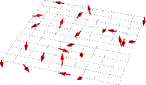
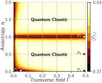
Figure 1: A random dipolar spin model on square lattice. Left: Dipoles localized in randomly selected lattice sites (schematic). Each dipole carries spin 1/2 and has a random orientation (red arrows) parametrized by uniformly distributed random angles $\theta$ and $\phi$. Right: Phase diagram of model in Eqs. (2)-(3) obtained from the energy level statistics of $N=10$ spins on $4\times 4$ lattice averaged over 500 disorder realization. False color shows the disorder averaged adjacent gap ratio $\langle\tilde{r}\rangle_{\text{\tiny$J$}}$ defined in the main text. In the quantum chaotic (bright) region $\langle\tilde{r}\rangle_{\text{\tiny$J$}}=0.53$ whereas $\langle\tilde{r}\rangle_{\text{\tiny$J$}}=0.37$ in the (dark) non-chaotic region. Four points, $\mathcal{P}_{1}$ to $\mathcal{P}_{4}$, are selected for detailed analysis which is presented below.

It remains unclear which experimental system can exhibit these intriguing properties. Several proposals have been put forward to realize the SYK model or its variants experimentally based on interacting fermions Chew et al. (2017); Pikulin and Franz (2017); Danshita et al. (2017); Chen et al. (2018); Marino and Rey (2018). The challenge is to engineer Majorana fermions or infinite-range coupling between complex fermions. In this paper, we follow an alternative route and seek to find a quantum spin model that shows fast scrambling and many-body quantum chaos similar to the SYK model. Previous numerical study of the transverse-field Sherrington-Kirkpatrick-Ising (SKI) model found exponential growth in the so-called out-of-time correlations (OTOC), but the growth exponent $\lambda_{L}$, called the Lyapunov exponent in the literature, is orders of magnitude smaller than the maximum bound Yao et al. (2016). Here, we propose to relax the assumption of infinite-range coupling as in SKI and SYK, and replace it with power-law interactions whose sign and magnitude depend on an on-site degree of freedom that can have quenched disorder. This leads us to a quantum spin model inspired by recent experiments on dipolar spin systems, e.g. quantum gases of polar molecules Yan et al. (2013) and magnetic atoms de Paz et al. (2013) confined in optical lattices and nitrogen-vacancy centers in diamond Choi et al. (2017). The dipole-dipole interaction naturally realizes long-ranged random (since it depends on the random orientation of the dipoles) exchange between spins.

We examine the spectral statistics and OTOC of the random dipolar spin model using exact diagonalization. In general, OTOC exhibits complicated time and temperature dependence including multiple regimes even for idealized models such as SYK Bagrets et al. (2017) or SKI Yao et al. (2016). There is no single formula that can fit all time scales or models. For example, power-law behavior of OTOC was noted in Ref. Chen et al. (2017) for several spin models. $\lambda_{L}$ for the complex fermion SYK model was found to be very small Fu and Sachdev (2016). Ref. Shen et al. (2017) reported that $\lambda_{L}$ reaches its maximum bound near the quantum critical points. Key to our analysis of $\lambda_{L}$ is a careful separation of the exponential growth from the power law saturation. While our model thermalizes slower than a black hole, we find it to be a surprisingly fast scrambler: in the limit of low temperature and large number of spins, $\lambda_{L}$ seems to approach the maximum bound.

II A dipolar spin model with random couplings

Consider a generic model Hamiltonian for spin 1/2 on square lattice

$$H_{\mathrm{d}}=\sum_{i>j}J_{ij}\biggr{[}\eta(\sigma_{i}^{x}\sigma_{j}^{x}+\sigma_{i}^{y}\sigma_{j}^{y})+\sigma_{i}^{z}\sigma_{j}^{z}\biggr{]}+\Gamma\sum_{i}\sigma^{x}_{i}.$$ (2)

Here $\sigma^{x,y,z}_{i}$ are the Pauli spin operators on site $i$, the sum is over all occupied sites $i$ and $j$, $\eta$ is the exchange anisotropy, and $\Gamma$ is an external field along the $x$-direction. In previous work, the exchange couplings $\{J_{ij}\}$ are assumed to be random with normal distribution and all-to-all, i.e., independent of $\mathbf{r}_{ij}=\mathbf{r}_{i}-\mathbf{r}_{j}$, the distance between two spins at site $i$ and $j$. We refer to model Eq. (2) with such $\{J_{ij}\}$ as the Sherrington-Kirkpatrick XXZ model. For $\Gamma=0$ and $\eta=1$, it reduces the SU(2) spin model considered in Bray and Moore (1980) and generalized to SU(N) by Sachdev and Ye Sachdev and Ye (1993). For $\eta=0$, it reduces to the SKI model studied in Ref. Yao et al. (2016).

We propose to study model Eq. (2) for the more realistic case where $\{J_{ij}\}$ are still random but decays as $|\mathbf{r}_{ij}|^{-3}$. To motivate such a scenario, imagine sprinkling $N$ dipoles, each carrying pseudospin 1/2, onto the square lattice. We allow empty sites but no double occupancy. Both the location and orientation of the sprinkled dipoles are assumed to be random as schematically shown in Fig. 1. These dipoles are localized with their orientations fixed. The coupling between spins are mediated by the dipolar interaction and takes the form

$$J_{ij}=\frac{J_{0}}{|\mathbf{r}_{ij}|^{3}}\biggr{[}\hat{d}_{i}\cdot\hat{d}_{j}-3(\hat{d}_{i}\cdot\hat{r}_{ij})(\hat{d}_{j}\cdot\hat{r}_{ij})\biggr{]}.$$ (3)

Here $\hat{r}_{ij}=\mathbf{r}_{ij}/|\mathbf{r}_{ij}|$, and the unit vector $\hat{d}_{i}$ specifies the orientation of the dipole at site $i$, $\hat{d}_{i}=(\sin\theta_{i}\cos\phi_{i},\sin\theta_{i}\sin\phi_{i},\cos\theta_{i})$ where angle $\theta_{i}$ ($\phi_{i}$) is random and uniformly distributed in $[0,\pi]$ ($[0,2\pi]$). The statistics of $J_{ij}$ given by Eq. (3) is sharply peaked at small exchanges and deviates significantly from normal distribution as shown in Fig. 4 of Appendix A. Roughly speaking, this is because there is more chance to find two spins of larger distance away (and hence small $J_{ij}$ values due to the power law decay). The model Eqs. (2)-(3) is an example of strongly disordered quantum many-body systems with long-range interaction, and our hypothesis is that it exhibits interesting scrambling dynamics. To test this hypothesis using numerics, we consider an $L\times L$ lattice with $N<L^{2}$ spins, and set the energy and inverse time units to be $J_{0}$ and $\hbar=k_{B}=1$.

In many experiments on dipolar spin systems, a magnetic or electric field is applied to orient all the dipole moments in the same direction $\hat{d}$ or to set a common quantization axis for the pseudospins. This leads to quantum spin models Keles and Zhao (2018a, b); Zou et al. (2017) where $J_{ij}$ is simplified to $J_{0}[1-(\hat{d}\cdot\hat{r}_{ij})^{2}]/|\mathbf{r}_{ij}|^{3}$. For randomly located dipoles $\mathbf{r}_{ij}$ with vacancies present, the resultant distributions of $J_{ij}$ is not symmetric (e.g., skewed towards negative couplings) and depends on the filling fraction of the lattice, making the system less ideal for studying scrambling dynamics. For this reason, we consider randomly oriented dipoles with stronger disorder described by Eq. (3). This requires random local fields to lock the dipole moments $\hat{d}_{i}$. Accordingly, the value of $\eta$ and $\Gamma$ may vary from site to site. For simplicity, we assume a constant value of $\eta$ and $\Gamma$ throughout the system.

III Spectral statistics

We first examine the energy level statistics of this model by exactly diagonalizing $H_{\mathrm{d}}$ for many random realizations of $\hat{d}_{i}$ for given anisotropy $\eta$ and transverse field $\Gamma$. Then, by varying $\eta$ and $\Gamma$, we can identify different regimes (“phases”) of this model by comparing its spectra with well known behaviors of disordered quantum many-body systems. We adopt the spectral measures proposed in Ref. Oganesyan and Huse (2007) which are widely used in the study of many-body localization in quantum systems Atas et al. (2013). Let $\{E_{n}\}$ be the sorted energy eigenvalues $E_{1}<E_{2}<E_{3}<\dots$ and $\Delta E_{n}=E_{n+1}-E_{n}$ the level spacing. Define the ratio of adjacent level spacing $r_{n}=\Delta E_{n}/\Delta E_{n-1}$ and $\tilde{r}_{n}=\mathrm{min}\left(r_{n},r_{n}^{-1}\right)$. For certain non-ergodic phases that do not thermalize, the energy levels are uncorrelated such that the probability distribution of $r_{n}$ follows Poisson distribution $\mathrm{P}(r)=1/(1+r)^{2}$. In comparison, for chaotic systems the energy levels repel each other giving rise to a probability distribution following Wigner-Dyson statistics $\mathrm{P}(r)=Z^{-1}(r+r^{2})^{b}/(1+r+r^{2})^{1+3b/2}$ where $Z$ and $b$ are constants depending on the ensemble symmetries. For example, $b=1$ and $Z=8/27$ for the Gaussian Orthogonal Ensemble (GOE). Note that the level statistics of the SYK model falls into the Wigner-Dyson category and has been studied in depth You et al. (2017). The left panel of Fig. 2 shows two examples of the computed $\mathrm{P}(r)$ for our model at the same $\eta$ but different $\Gamma$. They obey Poisson and GOE statistics respectively. Thus, this model has two distinctive phases.

The ensemble average of $\tilde{r}_{n}$, denoted by $\langle\tilde{r}_{n}\rangle_{\text{\tiny$J$}}$, serves as a convenient quantity to chart out the phase diagram, since $\langle\tilde{r}_{n}\rangle_{\text{\tiny$J$}}=0.37$ for Poisson statistics whereas $\langle\tilde{r}_{n}\rangle_{\text{\tiny$J$}}=0.53$ for GOE. As shown in the right panel of Fig. 2, the evolution of $\langle\tilde{r}_{n}\rangle_{\text{\tiny$J$}}$ indicates a transition from Poisson to GOE statistics for increasing $\Gamma$ in the Ising limit $\eta=0$. Even though only a smooth crossover can be seen in numerics with finite $N$, the variation of $\langle\tilde{r}_{n}\rangle_{\text{\tiny$J$}}$ becomes sharper as $N$ is increased. The crossing point of the $N=10$, $12$ and $14$ curves, $\Gamma_{c}\sim 0.1$, can be taken as a rough estimate of the phase boundary for $\eta=0$ in the thermodynamic limit $N\rightarrow\infty$. The estimated $\Gamma_{c}$ value is comparable to that of the Sherrington-Kirkpatrick model Suzuki et al. (2013); Yao et al. (2016). Similar result is shown on a modified SYK model recently García-García et al. (2018). We carry out scans on the $\eta-\Gamma$ plane for $N=10$ spins averaged over 500 random realizations. The computed $\langle\tilde{r}_{n}\rangle_{\text{\tiny$J$}}$ is illustrated in Fig. 1 (right panel) using false color where the bright regions feature quantum many-body chaos. We will use independent evidences below to further corroborate this claim. The non-chaotic regions cluster around the lines $\eta=1$ (Heisenberg limit) and $\eta=0$ (Ising limit) where the spin model enjoys higher symmetry. In what follows, we shall concentrate on the wide chaotic regime.

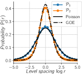
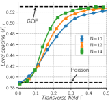
Figure 2: Energy level statistics of the random dipolar spin model in the Ising limit $\eta=0$. Left: Statistics of level spacing $r$ for points $\mathcal{P}_{1}$ and $\mathcal{P}_{2}$, calculated for 500 random realizations, $N=10$ and $L=4$. Also shown are the Poisson (solid line) and GOE (dashed line) distribution fuctions defined in the main text. For clarity, $\log r$ is used as the $x$-axis. Right: adjacent gap ratio $\langle\tilde{r}\rangle_{\text{\tiny$J$}}$ as a function of transverse field $\Gamma$ showing a transition to quantum chaos at critical point $\Gamma_{c}\sim 0.1$.

We have also computed the spectral form factor for $H_{d}$ which is shown in Appendix B. This quantity is defined as the disorder average $\langle|Z(t)|^{2}\rangle_{\text{\tiny$J$}}$, where $Z(t)={Z^{-1}_{0}}\sum_{n}e^{-itE_{n}}$ with $Z_{0}$ a normalization constant. It probes spectral correlations beyond nearest level spacing, and its time evolution shows a characteristic dip-ramp-plateau pattern for quantum chaotic systems. For example, the SYK model shows this behavior as discussed recently in Ref. Cotler et al. (2017a, b). Our results confirmed the presence of the dip-ramp-plateau feature in the spectral form factor within the bright regions in Fig. 1. This lends additional support for identifying them as regions of many-body chaos.

IV Out-of-time-order correlations

A direct diagnosis of many-body chaos is provided by the out-of-time-order correlations (OTOC). For two Hermitian operators $A$ and $B$, define Larkin and Ovchinnikov (1969)

$$C_{AB}(t)=-\langle[A(t),B(0)]^{2}\rangle,$$ (4)

where in the Heisenberg picture $A(t)=U^{\dagger}AU$ with $U=e^{-itH}$ the time evolution operator, and the angle bracket denotes thermal average $\langle\cdot\rangle\equiv\mathrm{Tr}(e^{-\beta H}\cdot)/\mathrm{Tr}e^{-\beta H}$ . In general, $C_{AB}(t)$ exhibits complex dynamics at intermediate times due to the fact that $A(t)$ and $B$ fail to commute Roberts and Swingle (2016). For example, the OTOC of the SYK model shows several distinct time scales Kitaev (2015); Maldacena et al. (2016); Bagrets et al. (2017). At early (pre-chaos) times up to a dissipation/collision time scale $t_{d}$, the dynamics can be captured by two-point correlators and the growth of OTOC is negligible. This is followed by an exponential growth $C_{AB}(t)\sim e^{\lambda_{L}t}$, where $\lambda_{L}$ is called the quantum Lyapunov exponent for convenience. Such growth is a signature of chaos. Interestingly, the saddle point solution of SYK in the large-N limit indicates that $\lambda_{L}$ saturates the conjectured bound $2\pi T$, pointing to a possible gravity dual of this model in the form of a black hole Maldacena et al. (2016). Recently, it was shown that at even later times, the OTOC of SYK crosses over to a universal power-law behavior containing $t^{-6}$ and its exact dynamics depends on temperature Bagrets et al. (2017).

To characterize many-body chaos in our model, we choose $A$ and $B$ as the local spin operators $\sigma_{i}^{z}$ and $\sigma_{j}^{z}$ and define

$$C(t)=\frac{1}{N(N-1)}\sum_{i\neq j}C_{\sigma^{z}_{i}\sigma^{z}_{j}}(t),$$ (5)

where the sum can be viewed as average over all sites. We compute the disorder average $\langle C(t)\rangle_{\text{\tiny$J$}}$ where $\langle\cdot\rangle_{J}$ denotes average over many random realizations. Fig. 3 shows the computed OTOC for a few selected points from the phase diagram (see Fig. 1 for the location of points $\mathcal{P}_{1}$ to $\mathcal{P}_{4}$) at two different temperatures. For point $\mathcal{P}_{1}$ which has Poisson level statistics, $\langle C(t)\rangle_{\text{\tiny$J$}}$ is very small and its growth is strongly suppressed for both temperatures. Our result is consistent with previous observations that the OTOC at infinite temperature grows at late times for many-body localized phases Huang et al. (2016); Chen et al. (2017); Fan et al. (2017). For point $\mathcal{P}_{3}$, which is deep inside the GOE (quantum chaotic) region, $\langle C(t)\rangle_{\text{\tiny$J$}}$ grows rapidly and saturates to the value of 2 in the long time limit. We will focus on this example and analyze its time and temperature dependence in details below. Note that the OTOC for point $\mathcal{P}_{2}$ resembles that of $\mathcal{P}_{3}$, but the increase of $\langle C(t)\rangle_{\text{\tiny$J$}}$ begins at a later time, and it takes longer to reach the saturation value of 2 especially at lower temperatures. Similar results were reported for the transverse-field SKI model Yao et al. (2016). While both rapid rise and saturation are observed for point $\mathcal{P}_{4}$, it falls short of reaching the saturation value 2.

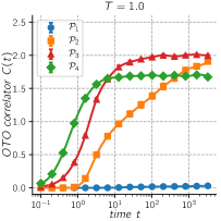
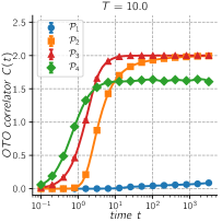
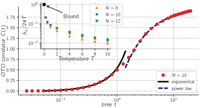
Figure 3: Out-of-time-order correlation $C(t)$ for the random dipolar spin model at high (top left) and low (top right) temperatures. The ensemble average $\langle C(t)\rangle_{\text{\tiny$J$}}$ (filled circles) are obtained for $N=10$ spins and averages are calculated over 500 disorder realizations. Lower panel: the time dependence of $\langle C(t)\rangle_{\text{\tiny$J$}}$ for point $\mathcal{P}_{3}$ and $T=1$ shows two distinct regimes. At early times, it shows exponential growth, fit to Eq. (6) (black solid line) yields the Lyapunov exponent $\lambda_{L}/(2\pi T)=0.13\pm 0.02$. The later time dynamics obeys a power-law Eq. (7), with $\mu=0.96\pm 0.01$ (dark blue dashed line). The inset shows the scaling of Lyapunov exponent with temperature for $N=8$, $N=10$ and $12$ spins. The black dot represents the conjectured bound for chaos, $\lambda_{L}/(2\pi T)=1$. The error bars are typically smaller than the marker sizes given in the figures.

We now extract the Lyapunov exponent from the numerics and study its temperature scaling, using point $\mathcal{P}_{3}$ deep inside the chaotic phase as an example. This will give a quantitative description of the scrambling dynamics, making it possible to assess how close our model is to the ideal limit set by SYK. We find that for early times, $t<t_{L}\sim 1$, the OTOC is well described by exponential growth,

$$C(t<t_{L})=C_{0}+\alpha_{L}e^{\lambda_{L}t},$$ (6)

where the fitting parameters $C_{0}$, $\alpha_{L}$ and $\lambda_{L}$ are obtained from non-linear least squares fit of the data. For the $T=1$ data shown in the lower panel Fig. 3, we find $\lambda_{L}\approx 0.13(2\pi T)$, below the bound $2\pi T$ as expected. Performing the same procedure for different temperatures, we obtain the corresponding values of $\lambda_{L}/2\pi T$. The result is summarized in the inset of Fig. 3. Interestingly, the extracted Lyapunov exponent of our system approaches the conjectured bound $\lambda_{L}/2\pi T=1$ in the low temperature limit .

The time dependence of OTOC after $t_{L}$ can no longer be described by exponential. Instead, we find that after a second time scale $t>t_{P}\sim 2$, the approach of OTOC to its saturation value is well described by a power law,

$$C(t>t_{P})=2-\alpha_{P}/t^{\mu},$$ (7)

where the parameters $\alpha_{P}$ and $\mu$ can be obtained from non-linear regression. We find $\mu\approx 0.96$ for the low temperature $T=1$ data shown in Fig. 3, whereas $\mu\approx 1.9$ for higher temperature $T=10$ (fit not shown). We note these values are quite far from the power-law exponent $\mu=6$ predicted for the SYK model in Ref. Bagrets et al. (2017). Because the power law is attributed to soft mode fluctuations, the value of $\mu$ can be model dependent.

To benchmark our numerics, we also computed the OTOC for the infinite-range Sherrington-Kirkpatrick XXZ model and compared it with the random dipolar spin model discussed above. The results are summarized in Fig. 7 of Appendix C. The extracted $\lambda_{L}$ from both cases shows a similar temperature dependence approaching the conjectured bound $2\pi T$ at low temperatures. This offers a hint that random power-law interactions may be sufficient for accessing fast scrambling and the possible existence of a universal, holographic dual theory at low energies similar to the SYK model Sachdev (2015). An interesting open problem is to compare the growth of entanglement entropy and information scrambling for models with different randomness, power laws, or spatial dimensions which is beyond the scope of our work. Such a systematic investigations using larger system sizes may reveal phenomena beyond the SYK model.

V Conclusion

In summary, the random dipolar spin model with power-law interactions proposed and studied here provides a concrete starting point to engineer spin systems that exhibit rich quantum many-body dynamics. The phase diagram obtained from corroborating the energy level statistics, spectral form factor, and out-of-time-order correlations points to a robust quantum chaotic phase in this model. And the OTOC is found to show rapid scrambling, i.e., exponential growth at early times, as well as power-law at late times. Dipolar quantum spin systems have been realized using polar molecules such as KRb confined in optical lattices where the pseudospin describes two rotational states of the molecules Yan et al. (2013); Hazzard et al. (2014); Gorshkov et al. (2011), or atoms with large magnetic moments where the spin refers to the hyperfine states de Paz et al. (2013). Dipolar spin models have also been achieved using nitrogen-vacancy centers in diamond Choi et al. (2017), nuclear spins Álvarez et al. (2015), trapped ions Bohnet et al. (2016) with tunable interactions Wilson et al. (2014), or Rydberg atoms Ravets et al. (2014). Steady progress has been made to control the exchange coupling Bermudez et al. (2017) and in-situ detection Covey et al. (2018). To realize the model proposed here, there remain two challenges. The first is better control of orientation randomness, possibly with a spatially quasi-periodic field. The second is to measure OTOC experimentally, which has been demonstrated recently for two types of quantum spin simulators Gärttner et al. (2017); Li et al. (2017). We hope our results can further stimulate experimental progress on dipolar spin quantum simulators.

Appendix A Statistics of exchange couplings

In the SYK model, the statistics of four fermion couplings $\{J_{ijkl}\}$ obeys normal distribution, they have zero mean and a constant standard deviation. Thanks to this, one can apply the replica trick and perform integration over couplings which yields an exact solution. The exchange couplings in infinite-range (e.g. Sherrington-Kirkpatrick) spin models studied so far also obey normal distribution. Application of the replica trick suggested a possible spin glass ground state Bray and Moore (1980). Ref. Sachdev and Ye, 1993 further generalize the SU(2) spin model to SU(N) spins and found a saddle point with disordered (spin liquid) state for large $N$.

We show the statistics of couplings $J_{ij}$ in Fig. 4 for the spin-1/2 model $H_{d}$ introduced in the main text based on randomly oriented dipolar spins. The histogram significantly deviates from Gaussian distributions (the orange curve is a Gaussian constructed using the mean and standard deviation from the data). It follows more closely the Cauchy-Lorentz distribution. This suggests that the replica trick may not be applied straightforwardly to $H_{d}$. To enhance quantum fluctuations and prevent a possible spin glass ground state, we include a transverse field and keep $\Gamma$ as a tuning parameter in our model.

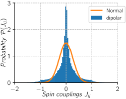
Figure 4: Statistics of dipolar spin exchange $J_{ij}$ generated from a few thousand random samples. For each sample, we consider $N=12$ dipolar spins localized in $4\times 4$ square lattice with random positions as well as random dipolar orientations. It deviates greatly from the normal distribution.

Appendix B Spectral Form Factor

Spectral form factor is defined as the thermal expectation value of time evolution operator $U=e^{-itH}$,

$$Z_{\beta}(t)=\mathrm{Tr}\left(e^{-\beta H-itH}\right)/\mathrm{Tr}(e^{-\beta H}),$$ (8)

where $H$ is the Hamiltonian under consideration, $t$ is time, and $\beta$ is the inverse temperature. Here we are interested in the infinite temperature limit, so we define $Z=Z_{\beta\rightarrow 0}$. In the energy eigen-basis, one can expand the trace to get

$$Z(t)=\frac{1}{Z_{0}}\sum_{n}e^{-itE_{n}}$$ (9)

where $Z_{0}$ is the normalization constant, and $E_{n}$ are the energy eigenvalues. At early times, $Z(t)$ approaches unity whereas at late times the phase factor inside the sum rapidly fluctuates. When ensemble average is taken, $Z(t)$ vanishes for large $t$. Therefore, it is more useful to study the modulus square of $Z(t)$,

$$|Z(t)|^{2}=\frac{1}{Z_{0}^{2}}\sum_{n,m}e^{-it(E_{n}-E_{m})}.$$ (10)

Notice that this quantity contains information about the level spacing $E_{n}-E_{m}$ which may obey non-trivial statistics such as Wigner-Dyson distribution. In addition, it also probes level correlations beyond the nearest neighbors in the energy level spectrum. This offers certain advantages over the level spacing measures $P(r)$ and $\tilde{r}_{n}$ discussed in the main text.

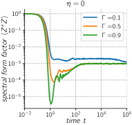
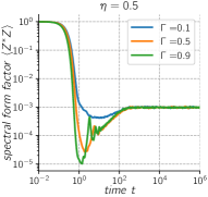
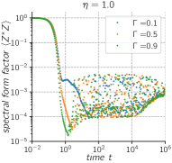
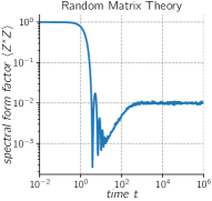
Figure 5: Spectral form factor of random dipolar spin model for 10 spins average over 1000 samples. We presented several constant $\eta$ cuts along the phase diagram which is indicated in the title. For reference, the result from GOE random matrix theory is presented on the fourth panel.

Spectral form factor has proven to be a useful tool for diagnosing many-body chaos in quantum systems. For example, several works have established that $|Z(t)|^{2}$ shows a robust dip-ramp-plateau behavior for the SYK model Cotler et al. (2017b, a). Such behavior is illustrated in the fourth panel of Fig. 5 for the Gaussian Orthogonal Ensemble in random matrix theory (with $100\times 100$ matrices and thousands of random samples) del Campo et al. (2017); Chenu et al. (2019). The ensemble average $\langle|Z(t)|^{2}\rangle$ decays rapidly at early time to reach a dip, followed by a ramp and then finally a plateau. The result is believed to be quite generic for quantum chaotic systems.

Fig. 5 shows the form factor of our spin model $H_{d}$ computed for a few representative cuts in the phase diagram. In the Ising limit $\eta=0$, shown on the first panel, $\langle{|Z|^{2}}\rangle$ decays directly to a constant value for $\Gamma=0.1$ with no dip feature (this point belongs to the non-chaotic phase in the phase diagram). For larger transverse field, e.g. $\Gamma=0.9$, the dip and ramp are fully developed indicating many-body chaos. At larger anisotropy $\eta=0.5$, similar result is obtained, and chaos is already manifest at $\Gamma=0.5$. Along the $\eta=1$ line (again within the non-chaotic phase), the form factor shows oscillations but no dip-ramp-plateau structure. These results are consistent with the level spacing analysis and unambiguously identify the two regions with and without many-body chaos in the phase diagram.

Note that the ramp connects the plateau region smoothly in the dipolar spin model without a kink or a cusp. This is consistent with GOE statistics as previously noted in Ref. Cotler et al. (2017b). In Fig. 7, we study the scaling of spectral form factor with total number of spins $N$. Different from the SYK model, smooth connection of ramp to plateau does not change with number of spins. This means our model is in GOE class independent of number of spins. Moreover, the early time oscillations of form factor around the dip seems to be fading away for larger $N$ which indicates stronger quantum chaos in $N\rightarrow\infty$ limit. The early time oscillations before the dip seen in the RMT form factor is the result of hard edges in the density of states (i.e. Wigner circle theorem). Similar oscillations also takes place in SYK model since it also has hard edges in the spectrum. Our model does not show this because of the long tails in the density of states. Finally we observe that the dip time grows slowly with large $N$, whereas plateau time seems to grow much faster. This is also similar to the result reported in Cotler et al. (2017b).

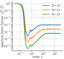
Figure 6: Scaling of the spectral form factor with the total number of spins in the random dipolar spin model at the quantum chaotic phase ($\mathcal{P}_{3}$ point in the phase diagram). Ensemble averages are calculated for 1000 random samples.

Appendix C Comparison with Sherrington-Kirkpatrick XXZ model

In the main text, we refer to $H_{d}$ in Eq. (1) with normally distributed $J_{ij}$, with zero mean and unit variance, as the Sherrington-Kirkpatrick XXZ model. Clearly, this model is more convenient for theoretical investigations. In this section, we discuss our results on the comparison of random dipolar spins with such a model with Gaussian distributed $J_{ij}$ as summarized in Fig. 4. Comparison of the OTOC between the Gaussian and dipolar spin models for low and high temperatures are shown in Fig. 7 where the last column shows the extracted Lyapunov exponents. Here we take $N=8$ and $L=4$ and calculate averages over $10^{3}$ samples and set $\Gamma=\eta=0.5$ which is the point $\mathcal{P}_{3}$ in Fig. 1. The figure shows that dipolar spin models exhibits a scrambling dynamics quite similar to Gaussian model for both low and high temperatures. Extraction of Lyapunov exponent via the same procedure explained in the main text also shows similar fast scrambling behavior in the infrared limit. Naturally, $\lambda_{L}$ of the Gaussian model seems to be slightly larger than the dipolar spin model.

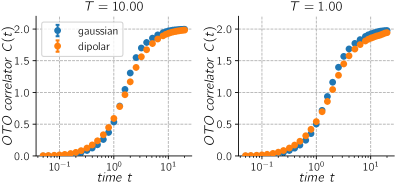
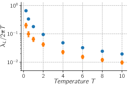
Figure 7: Comparison of OTOC of the random dipolar spins and the normally distributed random spins. Top left is high temperature OTOC whereas top right is the low temperature. Bottom panel shows the comparison of the scaling of Lyapunov exponent with the temperature. For both cases, OTOC is calculated for 8 spins averaged over 1000 random samples and $t\in[0.1,1]$ interval is used for fitting.

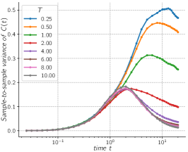
Figure 8: Sample-to-sample fluctuations of the OTOC function as a function of time at from low temperature $T=0.25$ to $T=10$ (Temperature increases from upper line to bottom line ).

Appendix D Sample-to-sample Fluctuations of OTOC

In this section we present our data regarding the sample-to-sample variance of out-of-time order correlation functions $\delta C^{2}(t)\equiv\langle C^{2}(t)\rangle_{\text{\tiny$J$}}-\langle C(t)\rangle_{\text{\tiny$J$}}^{2}$ where $\langle\cdot\rangle_{\text{\tiny$J$}}$ represent disorder averaging. Our results, in Fig. 8, show an interesting interplay between the time scales during the scrambling and the temperature. It turns out that the sample-to-sample variations increases at low temperature and is not a monotonic function of time. For example, at high temperatures there is an intermediate time scale where the variance reaches its maximum.

References

- Edwards and Anderson (1975) S. F. Edwards and P. W. Anderson, Journal of Physics F: Metal Physics 5, 965 (1975).
- Sherrington and Kirkpatrick (1975) D. Sherrington and S. Kirkpatrick, Phys. Rev. Lett. 35, 1792 (1975).
- Binder and Young (1986) K. Binder and A. P. Young, Rev. Mod. Phys. 58, 801 (1986).
- Sachdev and Ye (1993) S. Sachdev and J. Ye, Phys. Rev. Lett. 70, 3339 (1993).
- Kitaev (2015) A. Kitaev, “Hidden correlations in the Hawking radiation and thermal noise,” (2015).
- Maldacena and Stanford (2016) J. Maldacena and D. Stanford, Phys. Rev. D 94, 106002 (2016).
- Maldacena et al. (2016) J. Maldacena, S. H. Shenker, and D. Stanford, J. High Energy Phys. 2016, 106 (2016).
- Sekino and Susskind (2008) Y. Sekino and L. Susskind, Journal of High Energy Physics 2008, 065 (2008).
- Chew et al. (2017) A. Chew, A. Essin, and J. Alicea, Phys. Rev. B 96, 121119(R) (2017).
- Pikulin and Franz (2017) D. I. Pikulin and M. Franz, Phys. Rev. X 7, 031006 (2017).
- Danshita et al. (2017) I. Danshita, M. Hanada, and M. Tezuka, Progress of Theoretical and Experimental Physics 2017, 1093 (2017).
- Chen et al. (2018) A. Chen, R. Ilan, F. de Juan, D. I. Pikulin, and M. Franz, Phys. Rev. Lett. 121, 036403 (2018).
- Marino and Rey (2018) J. Marino and A. Rey, arXiv:1810.00866 (2018).
- Yao et al. (2016) N. Y. Yao, F. Grusdt, B. Swingle, M. D. Lukin, D. M. Stamper-Kurn, J. E. Moore, and E. A. Demler, (2016), arXiv:1607.01801 .
- Yan et al. (2013) B. Yan, S. A. Moses, B. Gadway, J. P. Covey, K. R. Hazzard, A. M. Rey, D. S. Jin, and J. Ye, Nature 501, 521 (2013).
- de Paz et al. (2013) A. de Paz, A. Sharma, A. Chotia, E. Maréchal, J. H. Huckans, P. Pedri, L. Santos, O. Gorceix, L. Vernac, and B. Laburthe-Tolra, Phys. Rev. Lett. 111, 185305 (2013).
- Choi et al. (2017) S. Choi, J. Choi, R. Landig, G. Kucsko, H. Zhou, J. Isoya, F. Jelezko, S. Onoda, H. Sumiya, V. Khemani, C. von Keyserlingk, N. Y. Yao, E. Demler, and M. D. Lukin, Nature 543, 221 (2017).
- Bagrets et al. (2017) D. Bagrets, A. Altland, and A. Kamenev, Nucl. Phys. B 921, 727 (2017).
- Chen et al. (2017) X. Chen, T. Zhou, D. A. Huse, and E. Fradkin, Ann. Phys. 529, 1600332 (2017).
- Fu and Sachdev (2016) W. Fu and S. Sachdev, Phys. Rev. B 94, 035135 (2016).
- Shen et al. (2017) H. Shen, P. Zhang, R. Fan, and H. Zhai, Phys. Rev. B 96, 054503 (2017).
- Bray and Moore (1980) A. J. Bray and M. A. Moore, J. Phys. C Solid State Phys. 13, L655 (1980).
- Keles and Zhao (2018a) A. Keles and E. Zhao, Phys. Rev. B 97, 245105 (2018a).
- Keles and Zhao (2018b) A. Keles and E. Zhao, Phys. Rev. Lett. 120, 187202 (2018b).
- Zou et al. (2017) H. Zou, E. Zhao, and W. V. Liu, Phys. Rev. Lett. 119, 050401 (2017).
- Oganesyan and Huse (2007) V. Oganesyan and D. A. Huse, Phys. Rev. B 75, 155111 (2007).
- Atas et al. (2013) Y. Y. Atas, E. Bogomolny, O. Giraud, and G. Roux, Phys. Rev. Lett. 110, 084101 (2013).
- You et al. (2017) Y.-Z. You, A. W. W. Ludwig, and C. Xu, Phys. Rev. B 95, 115150 (2017).
- Suzuki et al. (2013) S. Suzuki, J.-i. Inoue, and B. K. Chakrabarti, Quantum Ising Phases and Transitions in Transverse Ising Models, Lecture Notes in Physics, Vol. 862 (Springer, Berlin, Heidelberg, 2013).
- García-García et al. (2018) A. M. García-García, B. Loureiro, A. Romero-Bermúdez, and M. Tezuka, Phys. Rev. Lett. 120, 241603 (2018).
- Cotler et al. (2017a) J. Cotler, N. Hunter-Jones, J. Liu, and B. Yoshida, Journal of High Energy Physics 2017, 48 (2017a).
- Cotler et al. (2017b) J. S. Cotler, G. Gur-Ari, M. Hanada, J. Polchinski, P. Saad, S. H. Shenker, D. Stanford, A. Streicher, and M. Tezuka, Journal of High Energy Physics 2017, 118 (2017b).
- Larkin and Ovchinnikov (1969) A. Larkin and Y. N. Ovchinnikov, Sov Phys JETP 28, 1200 (1969).
- Note (1) The definition of here is the unregularized OTOC, which is well behaved for lattice models. For continuum models, it is better to use the regularized OTOC, see Ref. Maldacena et al. (2016).
- Roberts and Swingle (2016) D. A. Roberts and B. Swingle, Phys. Rev. Lett. 117, 091602 (2016).
- Huang et al. (2016) Y. Huang, Y.-L. Zhang, and X. Chen, Annalen der Physik 529, 1600318 (2016).
- Fan et al. (2017) R. Fan, P. Zhang, H. Shen, and H. Zhai, Science Bulletin 62, 707 (2017).
- Note (2) Care must be taken when extrapolating toward the limit of , below a critical temperature the system may enter a regime where chaos is absent with possible order, as demonstrated for the SYK model in Ref. [17].
- Sachdev (2015) S. Sachdev, Phys. Rev. X 5, 041025 (2015).
- Hazzard et al. (2014) K. R. A. Hazzard, B. Gadway, M. Foss-Feig, B. Yan, S. A. Moses, J. P. Covey, N. Y. Yao, M. D. Lukin, J. Ye, D. S. Jin, and A. M. Rey, Phys. Rev. Lett. 113, 195302 (2014).
- Gorshkov et al. (2011) A. V. Gorshkov, S. R. Manmana, G. Chen, E. Demler, M. D. Lukin, and A. M. Rey, Phys. Rev. A 84, 033619 (2011).
- Álvarez et al. (2015) G. A. Álvarez, D. Suter, and R. Kaiser, Science 349, 846 (2015).
- Bohnet et al. (2016) J. G. Bohnet, B. C. Sawyer, J. W. Britton, M. L. Wall, A. M. Rey, M. Foss-Feig, and J. J. Bollinger, Science 352, 1297 (2016).
- Wilson et al. (2014) A. C. Wilson, Y. Colombe, K. R. Brown, E. Knill, D. Leibfried, and D. J. Wineland, Nature 512, 57 (2014).
- Ravets et al. (2014) S. Ravets, H. Labuhn, D. Barredo, L. Béguin, T. Lahaye, and A. Browaeys, Nature Physics 10, 914 (2014).
- Bermudez et al. (2017) A. Bermudez, L. Tagliacozzo, G. Sierra, and P. Richerme, Phys. Rev. B 95, 024431 (2017).
- Covey et al. (2018) J. P. Covey, L. D. Marco, Ó. L. Acevedo, A. M. Rey, and J. Ye, New Journal of Physics 20, 043031 (2018).
- Gärttner et al. (2017) M. Gärttner, J. G. Bohnet, A. Safavi-Naini, M. L. Wall, J. J. Bollinger, and A. M. Rey, Nature Physics 13, 781 (2017).
- Li et al. (2017) J. Li, R. Fan, H. Wang, B. Ye, B. Zeng, H. Zhai, X. Peng, and J. Du, Phys. Rev. X 7, 031011 (2017).
- del Campo et al. (2017) A. del Campo, J. Molina-Vilaplana, and J. Sonner, Phys. Rev. D 95, 126008 (2017).
- Chenu et al. (2019) A. Chenu, J. Molina-Vilaplana, and A. del Campo, Quantum 3, 127 (2019).