SNAP: A semismooth Newton algorithm for pathwise optimization with optimal local convergence rate and oracle properties
Abstract
We propose a semismooth Newton algorithm for pathwise optimization (SNAP) for the LASSO and Enet in sparse, high-dimensional linear regression. SNAP is derived from a suitable formulation of the KKT conditions based on Newton derivatives. It solves the semismooth KKT equations efficiently by actively and continuously seeking the support of the regression coefficients along the solution path with warm start. At each knot in the path, SNAP converges locally superlinearly for the Enet criterion and achieves an optimal local convergence rate for the LASSO criterion, i.e., SNAP converges in one step at the cost of two matrix-vector multiplication per iteration. Under certain regularity conditions on the design matrix and the minimum magnitude of the nonzero elements of the target regression coefficients, we show that SNAP hits a solution with the same signs as the regression coefficients and achieves a sharp estimation error bound in finite steps with high probability. The computational complexity of SNAP is shown to be the same as that of LARS and coordinate descent algorithms per iteration. Simulation studies and real data analysis support our theoretical results and demonstrate that SNAP is faster and accurate than LARS and coordinate descent algorithms.
Keywords: KKT conditions, LASSO, Newton derivative, semismooth functions, sign consistency, superlinear convergence
2010 MR Subject Classification 62F12, 62J05, 62J07
1 Introduction
In this paper, we propose a semismooth Newton algorithm for pathwise optimization (SNAP) for regularized high-dimensional regression problems. We consider the linear regression model
| (1.1) |
where is a response vector, is a design matrix, is a vector of underlying regression coefficients, and is a vector of random errors. We assume without loss of generality that is centered and the columns of are centered and -normalized. For this model, the LASSO (Tibshirani, , 1996; Chen et al., 1998a, ) solves
| (1.2) |
where is a penalty parameter. Closely related to the LASSO is the elastic net (Enet) (Zou and Hastie, , 2005), which solves
| (1.3) |
This can be viewed as a regularized form of (1.2). Since is strongly convex for , the Enet solution is unique. This enables us to characterize the unique minimum 2-norm LASSO solution (1.2) as the limit of as (Proposition 3.2). In high-dimensional settings, it is nontrivial to efficiently solve (1.2) and (1.3) numerically since they are large scale nondifferentiable optimization problems.
The key ingredient of SNAP is a semismooth Newton algorithm (SNA), which is derived based on a suitable formulation of the KKT conditions. At each step in the iteration, the SNA works by first estimating the support of the solution based on a combination of the primal and dual information, and then finding the values of the nonzero coefficients on the support. Interestingly, our analysis shows that the SNA can be formally derived as a Newton algorithm based on the notion of Newton derivatives for nondifferentiable functions (Kummer, , 1988; Qi and Sun, , 1993; Ito and Kunisch, , 2008).
SNAP proceeds by running SNA along a grid of values: with the continuation strategy and warm start, where , and the integer are user given parameters. It is easy to implement and computationally stable. Moreover, our simulation studies indicate that SNAP is nearly problem independent, in the sense that the computational cost of using SNAP to approximate the solution path is , independent of the following aspects of the model, including the ambient dimension, sparsity level, correlation structure of the predictors, range of the magnitude of the nonzero regression coefficients and the noise level .
1.1 Contributions
The most popular algorithms for solving -regularized problems in the literature are mainly first order methods. It is natural to ask whether we can develop a second order method, i.e, Newton type method, which is a workhorse in low dimensional estimation, for such nonsmooth optimization problems which converges faster than first order methods. We give a definitive answer to this question via proposing the SNAP algorithm and developed a MATLAB package snap, which is available at http://faculty.zuel.edu.cn/tjyjxxy/jyl/list.htm.
We show that, for the LASSO, the SNA converges locally in just one step, which is obviously the best possible local convergence rate for any algorithms (Theorem 3.3). For the Enet, it converges locally superlinearly (Theorem 3.2). To the best of our knowledge, these are the best convergence rates for LASSO and Enet regularized regression problems with in the literature. Our computational complexity analysis shows that the cost of each iteration in SNA is , which is the same as most existing LASSO solvers, including LARS and coordinate descent algorithms. Hence, the overall cost of using SNA to find the unique minimizer of is still due to its superlinear convergence if it is warm started.
Another contribution of this paper is that we establish the statistical properties of SNAP in the Gaussian noise case. Specifically, we show that under certain regularity conditions on the design matrix , the solution sequence generated by SNAP enjoys the sign consistency property in finite steps if the minimum magnitude of the nonzero elements of is of the order , which is the optimal magnitude of detectable signal. We also establish a sharp upper bound in supreme norm for the estimation error of the solution sequence.
1.2 Related work
Osborne et al., (2000) showed that the LASSO solution path is continuous and piecewise linear as a function of . They proposed a Homotopy algorithm that defines an active set of nonzero variables at the current vertex then moves to a new vertex by adding a new variable to or removing an existing one from the active set. Efron et al., (2004) proposed the LARS algorithm to trace the whole solution path of (1.2) by omitting the removing steps in the Homotopy algorithm. Donoho and Tsaig, (2008) showed that, in the noiseless case with and under certain conditions on and , LARS (Homotopy) algorithm has the “-step” convergence property with the cost of . However, the convergence property of LARS is unknown when the noise vector is nonzero in the settings. Further connections of SNA with LARS, sure independence screening (Fan and Lv, , 2008), and active set tricks for accelerating coordinate descent (Tibshirani et al., , 2012) are discussed in Section 5.
Several authors have adopted a Gauss-Seidel type coordinate descent algorithm (CD-GS) (Fu, , 1998; Friedman et al., , 2007; Wu and Lange, , 2008; Li and Osher, , 2009), as well as Jacobi type coordinate descent (CD-J), or iterative thresholding (Daubechies et al., , 2004; She, , 2009) to solve (1.2). For the CD-GS proposed in Friedman et al., (2007), the results of Tseng, (2001), Saha and Tewari, (2013) and Yun, (2014) only ensure the convergence and sublinear convergence rate of the sequence of the objective functions , but not the sequence of the solutions . Since in high-dimensional settings with , the global minimizers are generally not unique, hence, it is not clear which minimizer the sequence generated from CD-GS iterations converges to. The CD-GS proposed in Li and Osher, (2009) and Tseng and Yun, (2009) with refined sweep rules is guaranteed to converge. Other widely used algorithms include proximal gradient descent (Nesterov, , 2005, 2013; Agarwal et al., , 2012; Xiao and Zhang, , 2013), alternative direction method of multiplier (ADMM) (Boyd et al., , 2011; Chen et al., , 2017; Han et al., , 2017), among others. For more comprehensive reviews of the literature on the related topics, see the review papers by Tropp and Wright, (2010), and Parikh and Boyd, (2014).
Agarwal et al., (2012) considered the statistical properties of the proximal gradient descent path. But their analysis required knowing , which is unknown or hard to estimate in practice. Although this can be remedied by using the techniques developed by Xiao and Zhang, (2013), it does not achieve the sharp error bound as SNAP does.
1.3 Notation
Some notation used throughout this paper are defined below. With we denote the usual norm of a vector . denotes the number of nonzero elements of . denotes the transpose of the covariate matrix and denotes the operator norm of induced by vector with 2-norm. 1 or 0 denote a vector or a matrix with elements all 1 or 0. Define . For any with length , we denote (or as the subvector (or submatrix) whose entries (or columns) are listed in . denotes submatrix of whose rows and columns are listed in and , respectively. We use , to denote the support and sign of a vector , respectively. We use , and to denote the identity matrix, the regularized Gram matrix and , respectively.
1.4 Organization
In Section 2 we provide a heuristic and intuitive derivation of SNA for solving (1.3) (including (1.2) as a special case by setting ) and describe SNA for pathwise optimization (SNAP). In Section 3 we establish the locally superlinear convergence rate of SNA for (1.3) and local one-step convergence for (1.2), and analyze the computational complexity of SNA. In Section 4 we provide the conditions for the finite-step sign consistency of SNAP and the upper bounds for the estimation error. In Section 5 we discuss the relations of SNA with LARS, SIS, and active set tricks for accelerating coordinate descent. The implementation detail and numerical comparison with LARS and coordinate descent methods are given in Section 6. We conclude in Section 7 with some comments and future work. The proofs of the main results and some background on Newton derivatives used for deriving SNA are included in the appendices.
2 A general description of SNAP
In this section we first give an intuitive description of the SNA for computing the LASSO and Enet solutions at a given and . We then describe the SNAP, which uses SNA for computing the solution paths with warm start and a continuation strategy.
2.1 Motivating SNA based on the KKT conditions
The key idea in the proposed algorithm is to iteratively identify the active set in the optimization using both the primal and dual information, then solve the problem on the active set. Here the primal is simply and its dual is . Recall and . For the LASSO, the expression of simplifies to , i.e., the correlation vector between the predictors and the residual. For any given , the KKT conditions (Proposition 3.3) assert that is the unique Enet solution if and only if the pair satisfies
| (2.3) |
where is the soft-threshold operator (Donoho and Johnstone, , 1995) acting on component wise, that is, with
| (2.4) |
The KKT conditions in (2.3) are stated in equalities using the soft-threshold operator, rather than in the usual inequality form or in terms of set-valued subdifferentials. This is the basis for our derivation of the SNA, which seeks to solve these nonsmooth equations.
To simplify the notation we drop the subscripts of and write them as , when it does not cause any confusion. By the second equation of (2.3) and the definition of the soft-threshold operator, we have
| (2.5) |
| (2.6) |
where
| (2.7) |
Substituting (2.5) into the first equation of (2.3) and observing is invertible, we can solve the resulting linear system to get
| (2.8) | |||||
| (2.9) |
Therefore, can be obtained from (2.5)-(2.6) and (2.8)-(2.9) if is known.
This naturally leads to the follow iterative algorithm for computing . Let be the primal and dual approximation of at the th iteration. Based on (2.7), we approximate the active and inactive sets by
| (2.10) |
Based on (2.5)-(2.6) and (2.8)-(2.9) we obtain the updated approximation ,
| (2.11) | ||||
| (2.12) | ||||
| (2.13) | ||||
| (2.14) |
In (2.12) we introduce a (small) shifting parameter with and use a slightly more general version of (2.6), replacing with in (2.6). For , we solve a less shrunk version of the Enet. For the solution sequence with a suitable , we show that it achieves finite-step sign consistency and sharp estimation error bound (Theorem 4.1).
Summing up the above discussion, we get the SNA for minimizing (1.3) in Algorithm 1 below, where we write for a fixed .
Remark 2.1.
In the algorithm, we use a safeguard maximum number of iterations that can be defined by the user. We usually set due to the locally superlinear/one-step convergence of SNA.
Each line in Algorithm 1 consists of simple vector and matrix multiplications, except (2.13) in line 6, where we need to invert a matrix. Note that is usually a small subset of if Algorithm 1 is warm started. Intuitively, at the th step in the iteration, this algorithm tries to identify , an approximation of the underlying support by using the estimated coefficients with a proper adjustment determined by the KKT, and solves a low-dimensional adjusted least squares problem on . Therefore, with a good starting estimation of , which is guaranteed by using a continuation strategy with warm start described below, Algorithm 1 can find a good solution in a few steps. In Section 3, we derive Algorithm 1 formally from the semismooth Newton method and show that its convergence rate is locally superlinear for the Enet and locally one step for the LASSO.
2.2 Solution path approximation
We are often interested in the whole solution path of (1.3) for and some given . Here we approximate the solution path by computing on a given finite set for some integer , where . Obviously, satisfies (2.3) and (2.3) if . Hence we set , , and , where .
We adopt a simple continuation technique with warm start in computing the solution path. This strategy has been successfully used for computing the LASSO and Enet paths (Friedman et al., , 2007; Jiao et al., , 2017). We use the solution at as the initial value for computing the solution at . The shift parameter can be vary at different path knots , so here we use to demonstrate this. We summarize this in the following SNAP algorithm
3 Derivation of SNA and convergence analysis
3.1 KKT conditions
In this subsection, we first discuss the relationship between the minimizers of (1.2) and (1.3). We then characterize the unique minimizer (1.3) by its KKT system.
Proposition 3.1.
Let be the set of the LASSO solutions given in (1.2). Then is nonempty, convex and compact.
In general, the uniqueness of the LASSO solution (the minimizer of (1.2)) cannot be guaranteed in the settings. But the one in with the minimum Euclidean norm denoted by is unique. We have the following relation between and the Enet solutions .
Proposition 3.2.
For , the Enet (1.3) admits a unique minimizer denoted by . Furthermore, as .
By Proposition 3.2, a good numerical solution of (1.3) is a good approximation of the minimum 2-norm minimizer of (1.2) for a sufficiently small .
Proposition 3.3.
Here the KKT conditions are formulated in terms of equalities (2.3), which are different from but equivalent to the usual inequality form
where, and The reason we adopt the equation form (2.3) is that we can transform the minimization problem (1.3) into a root finding problem, which help us derive SNA formally under the framework of semismooth Newton method.
3.2 SNA as a Newton algorithm
We now formally derive the SNA based on the KKT conditions by using the semismooth Newton method (Kummer, , 1988; Qi and Sun, , 1993; Ito and Kunisch, , 2008) for finding a root of a nonsmooth equation. This enables us to prove its locally superlinear convergence stated in Theorem 3.2 below. The definition and related property on Newton derivative are given in Appendix A.
Let
where
By Proposition 3.3, to find the minimizer of (1.3), it suffices to find a root of . Although the classical Newton algorithm cannot be applied directly since is not Fréchet differentiable, we can resort to semismooth Newton algorithm since is Newton differentiable.
Let
We reorder such that . We also reorder and accordingly,
We have the following result concerning the Newton derivative of .
Theorem 3.1.
is Newton differentiable at any point . And
| (3.1) |
Furthermore, is invertible and is uniformly bounded with
At the iteration, the semismooth Newton method for finding the root of consists of two steps.
-
(1)
Solve for , where is an element of .
-
(2)
Update , set and go to step (1).
This has the same form as the classical Newton method, except that here we use an element of in step (1). Indeed, the key to the success of this method is to find a suitable and invertible . We state this method in Algorithm 3.
| (3.2) |
| (3.3) |
Remark 3.1.
When holds for some , Algorithm 1 converges. Hence it is natural to stop Algorithm 1 accordingly. A common condition that can be used as a stop rule of Algorithm 3 is when is sufficiently small, since this algorithm is a root finding process. Therefor we can use both stopping rules in Algorithm 1 due to the equivalence of Algorithm 1 and Algorithm 3. We also stop Algorithm 1 when the iteration number exceeds a prespecified integer .
It can be verified that Algorithm 1 with is just Algorithm 3 written in a form for easy computational implementation. The details are given in Appendix C. Thus it is indeed a semismooth Newton method. The more compact form of Algorithm 3 is better suited for its convergence analysis.
Theorem 3.2.
Theorem 3.2 shows the local supperlinear convergence rate of SNA, which is a superior property of Newton type algorithms to first order methods.
Theorem 3.3.
3.3 Computational complexity analysis
We now consider the computational complexity of SNA (Algorithm 1). We look at the number of floating point operations per iteration. Clearly it takes flops to finish step 4-7 in Algorithm 1. For step 8, we solve the linear equation iteratively by conjugate gradient (CG) method initialized with the projection of the previous solution onto the current active set (Golub and Van Loan, , 1996). The main operation of iteration of CG is two matrix-vector multiplication cost flops Therefore we can control the number of CG iterations smaller than to make that flops will be enough for step 8. For step 9, calculation of the matrix-vector product costs flops. So the the overall cost per iteration of Algorithm 1 is which is also the cost for state-of-the-art first order LASSO solvers. The local superlinear/one step convergence of SNA guaranteed that a good solution can be found in only a few iteration if it is warm started. Therefore, at each knot of the path, the whole cost of SNA can be still if we use the continuation strategy. So Algorithm 2 (SNAP) can get the solution path accurately and efficiently at the cost of with be the number of knot on the path, see the numerical results in Section 6.
4 Error bounds and finite-step sign consistency
As shown in Theorems 3.2 and 3.3, SNA converges locally superlinearly for Enet and converges in one step for LASSO. In this section we prove that the simple warm start technique makes the SNAP converge globally under certain mutual coherence conditions on and a condition on the minimum magnitude of the nonzero components of . Specifically, we show that SNAP hits a solution with the same sign as and attains a sharp statistical error bound in finitely many steps with high probability if we properly design the path and run SNA along it with warm start.
We only consider the LASSO, so we set and . The mutual coherence defined as (Donoho and Huo, , 2001; Donoho et al., , 2006) characterizes the minimum angle between different columns of . Let and . Define Denote the universal threshold value by . Let , , and , .
We make the following assumptions on the design matrix , the target coefficient , and the noise vector .
-
(A1)
The mutual coherence satisfies .
-
(A2)
The smallest nonzero regression coefficient satisfies .
-
(A3)
satisfies .
Lemma 4.1.
Suppose that (A1) to (A3) hold. There exists an integer such that and hold with probability at least .
Theorem 4.1.
Suppose that (A1) to (A3) hold. Then with probability at least , with , determined in Lemma 4.1, , and at the knot, has a finite step sign consistence property and achieves a sharp estimation error, i.e.,
| (4.1) |
and
| (4.2) |
Remark 4.1.
The properties of LASSO have been studied by many authors. For example, Zhao and Yu, (2006) and Meinshausen and Bühlmann, (2006) showed that LASSO is sign consistent under a strong irrepresentable condition, which is a little weaker than (A1). They also required be bounded below by with , which is stronger than (A2). Zhang and Huang, (2008) required satisfy a sparse Rieze condition, which may be weaker than (A1); and larger than , which is stronger than (A2). Wainwright, (2009) assumed a condition stronger than the strong irrepresentable condition to guarantee the uniqueness of LASSO and its sign consistency with a condition on similar to (A1). Lounici, (2008) and Candès and Plan, (2009) assumed the mutual coherence conditions with and for a constant , respectively; and their requirements for are similar to (A1) with different constants. In deriving the and error bounds of the LASSO, Donoho et al., (2006) and Zhang, (2009) assumed and , respectively. The latter is exactly (A1). However, these existing results do not imply the finite-step sign consistency property established in Theorem 4.1.
All the results mentioned above concern the minimizer of the LASSO problem, but they did not directly address the statistical properties of the sequence generated by a specific solver. So there is a gap between those theoretical results and the computational solutions. There has been efforts to close this gap. For example, Agarwal et al., (2012) considered the statistical properties of the proximal gradient descent path. But their analysis required knowing , which is hard to estimate in practice. Xiao and Zhang, (2013) remedied this, but their result does not achieve the sharp error bound like SNAP does. Also, the technique used for deriving the statistical properties of SNAP (a Newton type method), is quite different from the proximal gradient method (a gradient type method).
5 Connections LARS, SIS and active set tricks for accelerating coordinate descent
The key idea in SNAP is using the Newton type method SNA to iteratively identify the active set using both the primal and dual information, then solve the problem on the active set. In this section we discuss the connections between SNAP with other three dual active set mehtods, i.e., LARS, SIS (Fan and Lv, , 2008), and sequential strong rule SSR (active set tricks for accelerating coordinate descent) (Tibshirani et al., , 2012).
LARS (Efron et al., , 2004) also does not solve (1.2) exactly since it omits the removing procedure of Homotopy (Osborne et al., , 2000). As discussed in Donoho and Tsaig, (2008), the LARS algorithm can be formulated as
where is the set of the indices of the variables with highest correlation with the current residual, , , , and is the step size to the next breakpoint on the path (Efron et al., , 2004; Donoho and Tsaig, , 2008). Comparing Algorithm 2 (SNAP) (by setting ) with the above reformulation of the LARS algorithm, we see that both SNAP and LARS can be understood as approaches for estimating the support of the underlying solution, which is the essential aspect in fitting sparse, high-dimensional models. So, SNAP and LARS share some similarity both in formulation and in spirit although they were derived from different perspectives. However, the definitions of the active set in SNAP is based on the sum of primal approximation (current approximation ) and the dual approximation (current correlation ) while LARS is based on dual only. The following low-dimensional small noise interpretation may clarify the difference between the two active set definitions. If identity and we get
and
In addition, LARS selects variables one by one while SNAP can selects more than one variable at each iteration. Also, the adjusted least squares fits on the active sets in SNAP and LARS are different. Under certain conditions on both of them recover exactly in the noise free case (Donoho and Tsaig, , 2008) even when . But the convergence or consistency of LARS is unknown when the noise vector .
Given a starting point , SNA is initialized with . Therefore,
Thus the first active set generated by SNAP contains the features that coorelated with y larger than , which are the same as those from the sure independence screening (Fan and Lv, , 2008) with parameter and include the one selected by the first step of LARS. We then use (2.11) - (2.14) to obtain , and update the active set to using (2.10). Clearly, for , are determined not just by the correlation , but by the primal () and dual () together.
Tibshirani et al., (2012) proposed a sequential strong rule (SSR) for discarting predictors in LASSO-type problems. At point on the solution path, this rule discards the th predictor if
where for the LASSO penalty. They define active set
and set for and solve the LASSO problem on . By combining with a simple check of the KKT condition, it speeds up the computation considerably. So SNA shares some similarity in spirit with SSR in that both methods seek to identify an active set and solve a smaller optimization problem, although they are derived from quite different perspectives. However, there are some important differences. First, the active sets are determined differently. Specifically, SSR determines the active set only based on the dual approximation; while SNA uses both primal and dual approximation. Second, SNA does not need the unit slope assumption, and additional check of the KKT conditions is not needed (The cost of check KKT is ). Third, as far as we know, the statistical properties of the solution sequence generated from SSR are unknown, while error bounds and sign consistency are established under suitable conditions for the solution sequence generated from the SNAP.
6 Numerical examples
In this section, we present numerical examples to evaluate the performance of the proposed SNAP algorithm 2 for solving LASSO. All experiments are performed in MATLAB R2010b on a quad-core laptop with an Intel Core i5 CPU (2.60 GHz) and 8 GB RAM running Windows 8.1 (64 bit).
6.1 Comparison with existing popular algorithms
Both the LARS (Efron et al., , 2004; Donoho and Tsaig, , 2008) and the CD (Friedman et al., , 2007, 2010) are popular algorithms capable of efficiently computing the LASSO solution, hence we compare the proposed SNAP with these two algorithms. In implementation, we consider two solvers: (1) SolveLasso, the Matlab code for LARS with the LASSO modification, available online at http://sparselab.stanford.edu/SparseLab_files/Download_files/SparseLab21-Core.zip; (2) glmnet, the Fortran based Matlab package using CD, available online at https://github.com/distrep/DMLT/tree/master/external/glmnet. The parameters in the solvers are the default values as their online versions. In addition to the default stopping parameters in the solvers, we stop LARS (SolveLasso), CD (glmnet) and SNAP if the number of nonzero elements at some iteration is larger than a given fixed quantity such as or even larger , since the upper bound of the estimated sparsity level of LASSO is when (Candès et al., , 2006; Candès and Tao, , 2006).
6.2 Tuning parameter selection
To choose a proper value of in (1.2) is a crucial issue for LASSO problems, since it balances the tradeoff between the data fidelity and the sparsity level of the solution. In practice, the Bayesian information criterion (BIC) is a widely used selector for the tuning parameter selection, due to its model selection consistency under some regularity conditions. We refer the readers to Wang et al., (2007); Chen and Chen, (2008); Wang et al., (2009); Chen and Chen, (2012); Kim et al., (2012); Wang et al., (2013) and references therein for more details. In this paper, we use a modified BIC (MBIC) from Kim et al., (2012) to choose , which is given as
| (6.1) |
where is the candidate set for , and is the model identified by . Besides, the high-dimensional BIC (HBIC) in Wang et al., (2013) defined by
| (6.2) |
is also a good candidate for the selection of . Unless otherwise specified, the MBIC (6.1) is the default one to select .
6.3 Simulation
6.3.1 Implementation setting
The design matrix is generated as follows.
-
(i)
Classical Gaussian matrix with correlation parameter . The rows of are drawn independently from with , .
-
(ii)
Random Gaussian matrix with auto-correlation parameter . First we generate a random Gaussian matrix with its entries following i.i.d. . Then we define a matrix by setting ,
and .
The elements of the error vector are generated independently with , . Let be the support of , and let be the range of magnitude of nonzero elements of . The underling regression coefficient vector is generated in a way that is a randomly chosen subset of with . As in Becker et al., (2011), Shi et al., 2018b and Shi et al., 2018a , each nonzero entry of is generated as follows:
| (6.3) |
where , with probability and is uniformly distributed in . Then the observation vector . For convenience, we use and to denote the data generated as above, respectively.
6.3.2 The behavior of the SNAP algorithm
6.3.2.1 The algorithm parameters of SNAP
We study the influence of the free parameters and in the SNAP algorithm on the exact support recovery probability (Probability for short), that is, the percentage of the estimated model agrees with the true model . To this end, we independently generate datasets from for each combination of . Here means the sparsity level starts from to with an increment of . The numerical results are summarized in Figure 1, which consider the following two settings: (a) , and varying ; (b) , and varying .
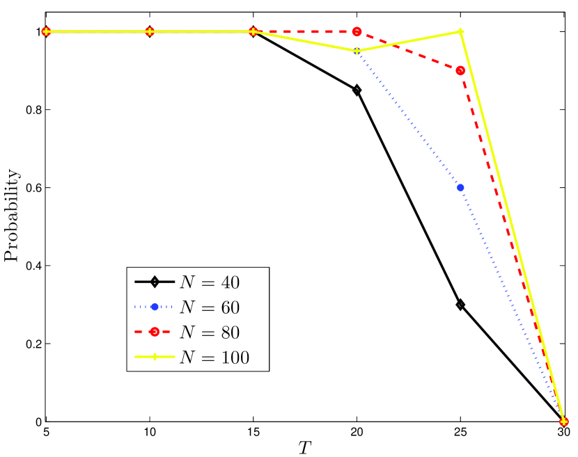
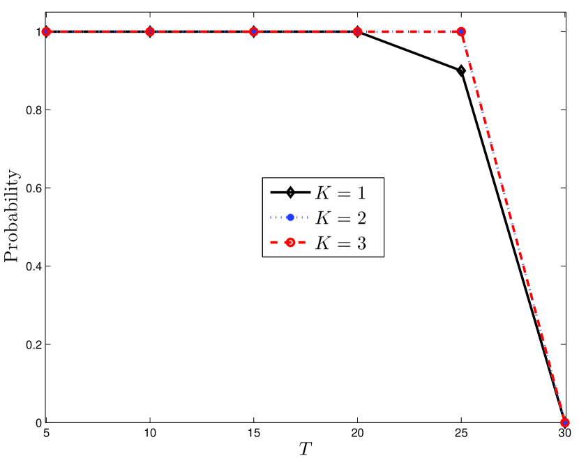
It is observed from Figure 1 that the influence of is very mild on the exact support recovery probability and generally works well in practice, due to the locally superlinear convergence of SNA and the continuation technique with warm start on the solution path, which is consistent with the conclusions in Section 2. It is also found in Figure 1 that Larger values make the algorithm have better exact support recovery probability, but the enhancement decreases as increases. Thus, unless otherwise specified, we set for the SNAP solver.
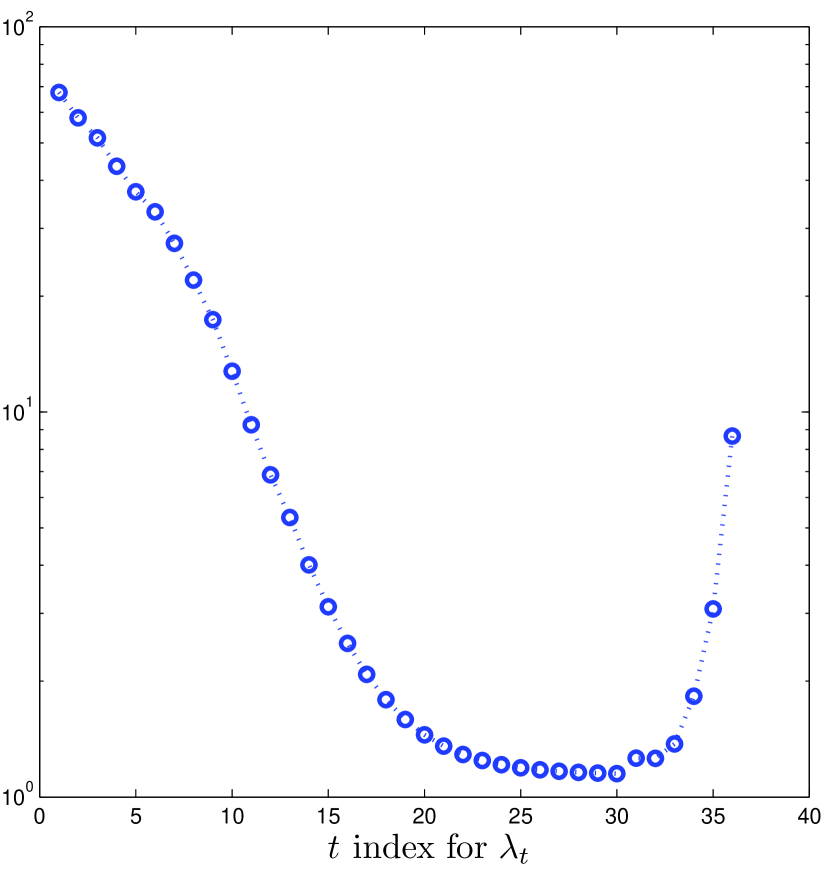
6.3.2.2 The MBIC selector for SNAP
We illustrate the performance of the MBIC selector (6.1) for SNAP with simulated data . The results are summarized in Figure 2. It can be observed from Figure 2 that the MBIC selector performs very well for the SNAP algorithm on the continuation solution path introduced in Section 2.2.
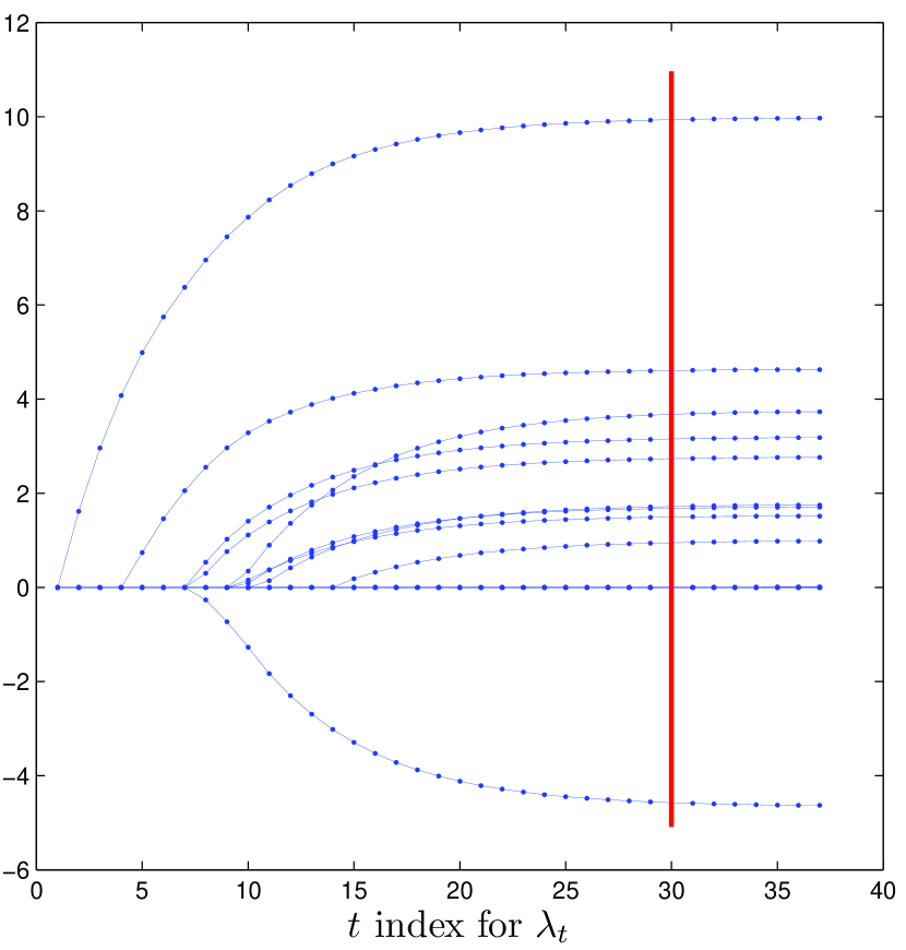
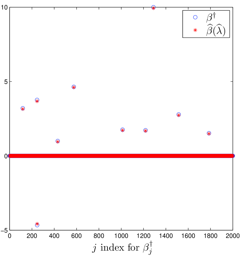
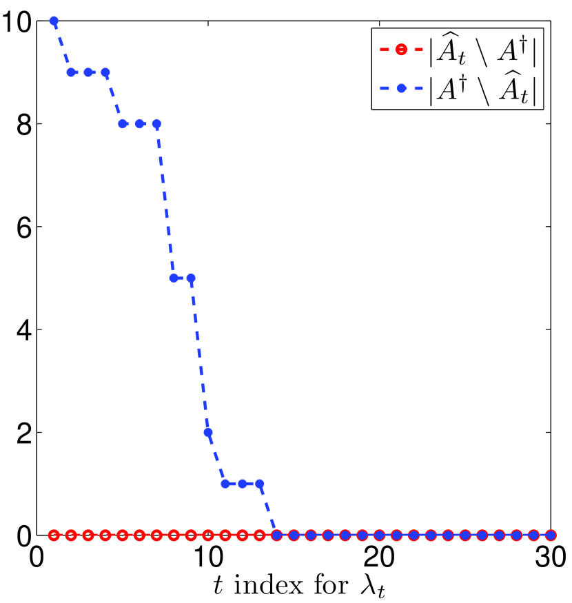
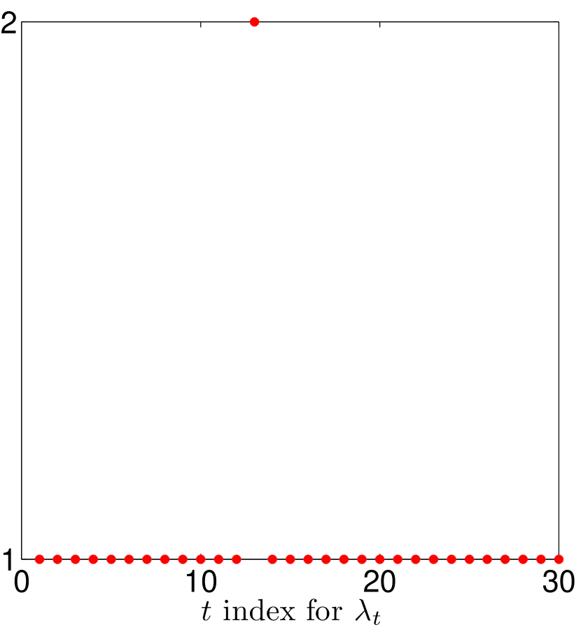
6.3.2.3 The local superlinear convergence of SNAP
To gain further insight into the SNAP algorithm, we illustrate the convergence behavior of the algorithm using the simulated data as that of Figure 2. Let , where is the solution to the -problem. Set . The convergence history is shown in Figure 3, which presents the change of the active sets and the number of iterations for each fixed along the path . It is observed in Figure 3 that , and the size increases monotonically as the path proceeds and eventually equals the true model size . In particular, for each problem with as the initial guess, SNAP generally reaches convergence within two iterations (typically one, noting that the maximum number of iterations here). This is attributed to the local superlinear/one step convergence of the algorithm for LASSO, which is consistent with the results in Theorem 3.3. Hence, the overall procedure is very efficient.
6.3.3 Efficiency and accuracy
To evaluate the efficiency and accuracy of the proposed SNAP algorithm, we independently generate datasets from two settings: (i) the classical Gaussian matrix with ; (ii) the random Gaussian matrix with . Based on independent runs, we compare SNAP with CD and LARS in terms of the average CPU time (Time, in seconds), the estimated average model size (MS) , the proportion of correct models (CM, in percentage terms) , the average absolute error (AE) , and the average relative error (RE) . The measure Time reflects the efficiency of the solvers, while measures MS, CM, AE and RE evaluate the accuracy (quality) of the solutions. Simulation results are summarized in Table 6.1 and Table 6.2, respectively.
| Method | Time | MS | CM | AE | RE | ||
|---|---|---|---|---|---|---|---|
| 0.3 | 0.2 | CD | 0.2287(0.0060) | 41.35(1.1135) | 23%(0.4230) | 0.1270(0.0286) | 0.0172(0.0042) |
| LARS | 0.2066(0.0336) | 41.25(1.1315) | 29%(0.4560) | 0.1208(0.0273) | 0.0163(0.0039) | ||
| SNAP | 0.1784(0.0111) | 40.07(0.2932) | 94%(0.2387) | 0.0808(0.0192) | 0.0105(0.0030) | ||
| 0.4 | CD | 0.2233(0.0023) | 42.71(1.5973) | 8%(0.2727) | 0.2041(0.0349) | 0.0275(0.0047) | |
| LARS | 0.2121(0.0316) | 42.14(3.0978) | 13%(0.3380) | 0.2672(0.6802) | 0.0344(0.0767) | ||
| SNAP | 0.1569(0.0041) | 40.23(0.4894) | 80%(0.4020) | 0.1528(0.0309) | 0.0200(0.0046) | ||
| 0.5 | 0.2 | CD | 0.2272(0.0025) | 42.74(1.8836) | 11%(0.3145) | 0.1484(0.0454) | 0.0193(0.0057) |
| LARS | 0.2086(0.0318) | 42.53(2.0863) | 15%(0.3589) | 0.1808(0.2411) | 0.0223(0.0317) | ||
| SNAP | 0.1746(0.0036) | 40.19(0.4861) | 84%(0.3685) | 0.0925(0.0319) | 0.0117(0.0039) | ||
| 0.4 | CD | 0.2236(0.0027) | 44.48(2.1057) | 0%(0.0000) | 0.2333(0.0616) | 0.0299(0.0066) | |
| LARS | 0.2162(0.0364) | 43.58(5.0835) | 1%(0.1000) | 0.3518(0.9235) | 0.0427(0.1029) | ||
| SNAP | 0.1548(0.0039) | 40.62(0.8138) | 55%(0.5000) | 0.1693(0.0439) | 0.0213(0.0045) | ||
| 0.7 | 0.2 | CD | 0.2280(0.0023) | 47.96(3.2315) | 0%(0.0000) | 0.2062(0.0956) | 0.0223(0.0061) |
| LARS | 0.2325(0.0317) | 47.85(3.4855) | 0%(0.0000) | 0.3177(0.6256) | 0.0255(0.0219) | ||
| SNAP | 0.1737(0.0047) | 41.25(1.2340) | 34%(0.4761) | 0.1274(0.0596) | 0.0136(0.0040) | ||
| 0.4 | CD | 0.2249(0.0023) | 50.59(3.6517) | 0%(0.0000) | 0.3323(0.1500) | 0.0349(0.0081) | |
| LARS | 0.2437(0.0310) | 50.61(5.4028) | 0%(0.0000) | 0.5283(0.7663) | 0.0463(0.0679) | ||
| SNAP | 0.1561(0.0040) | 41.92(1.4885) | 16%(0.3685) | 0.2337(0.0914) | 0.0245(0.0054) |
For each combination, it can be observed from Table 6.1 that SNAP has better speed performance than CD and LARS. With fixed, the CPU time of CD and SNAP slightly decreases as increases, while higher increases the timing of LARS in general. Given , the CPU time of CD and SNAP is relatively robust with respect to , while that of LARS generally increases as increases. According to MS, all solvers tend to overestimate the true model and SNAP usually selects a smaller model, while SNAP can select the correct model far more frequently than CD and LARS in terms of CM. The errors of all solvers AE and RE are small, which means they all can produce estimates that are very close to the true values of , while the AE and RE of SNAP are smaller than that of the other two, indicating that SNAP is generally more accurate than CD and LARS. Unsurprisingly, larger or will degrade the accuracy of all solvers. In addition, it is shown from Table 6.1 that SNAP generally has smaller ((or comparable) standard errors, especially in accuracy metrics MS, AE and RE, which means the results of SNAP are stable and robust. Similar phenomena also hold for the random Gaussian matrix setting in Table 6.2. In particular, since the value of is large in Table 6.2, the timing advantage of SNAP is more obvious, which implies that SNAP is capable of handling much larger data sets. In summary, SNAP behaves very well in simulation studies and generally outperforms the state-of-the-art solvers such as LARS and CD in terms of both efficiency and accuracy.
| Method | Time | MS | CM | AE | RE | ||
|---|---|---|---|---|---|---|---|
| 0.3 | 0.2 | CD | 1.6607(0.0185) | 51.59(1.5511) | 26%(0.4408) | 0.0902(0.0229) | 0.0121(0.0027) |
| LARS | 1.0458(0.1729) | 51.48(1.5007) | 29%(0.4560) | 0.0859(0.0215) | 0.0116(0.0027) | ||
| SNAP | 0.8685(0.0289) | 50.08(0.3075) | 93%(0.2564) | 0.0553(0.0133) | 0.0072(0.0017) | ||
| 0.4 | CD | 1.6416(0.0074) | 52.76(1.8916) | 9%(0.2876) | 0.1403(0.0314) | 0.0184(0.0031) | |
| LARS | 1.1354(0.2245) | 52.40(2.0792) | 12%(0.3266) | 0.1560(0.2001) | 0.0204(0.0272) | ||
| SNAP | 0.7764(0.0149) | 50.28(0.5519) | 76%(0.4292) | 0.1007(0.0217) | 0.0128(0.0022) | ||
| 0.5 | 0.2 | CD | 1.6719(0.0058) | 55.71(2.6678) | 0%(0.0000) | 0.0959(0.0583) | 0.0111(0.0028) |
| LARS | 1.1819(0.2301) | 55.59(3.3937) | 0%(0.0000) | 0.2002(0.4392) | 0.0164(0.0377) | ||
| SNAP | 0.8980(0.0108) | 50.82(1.0767) | 49%(0.5024) | 0.0559(0.0320) | 0.0064(0.0019) | ||
| 0.4 | CD | 1.6504(0.0064) | 57.86(3.0847) | 0%(0.0000) | 0.1583(0.1068) | 0.0164(0.0044) | |
| LARS | 1.3180(0.2388) | 56.85(4.2530) | 0%(0.0000) | 0.1954(0.4346) | 0.0220(0.0584) | ||
| SNAP | 0.8098(0.0172) | 51.20(1.1192) | 31%(0.4648) | 0.1091(0.0674) | 0.0112(0.0028) | ||
| 0.7 | 0.2 | CD | 1.6962(0.0100) | 65.22(4.6113) | 0%(0.0000) | 0.1411(0.1521) | 0.0114(0.0060) |
| LARS | 1.4585(0.2683) | 64.90(7.2202) | 0%(0.0000) | 0.5015(1.0090) | 0.0249(0.0411) | ||
| SNAP | 0.9439(0.0506) | 53.09(1.7529) | 6%(0.2387) | 0.0858(0.1374) | 0.0068(0.0100) | ||
| 0.4 | CD | 1.6715(0.0090) | 67.12(4.8996) | 0%(0.0000) | 0.1880(0.2146) | 0.0156(0.0082) | |
| LARS | 1.5399(0.2448) | 67.07(6.4499) | 0%(0.0000) | 0.5493(0.9422) | 0.0271(0.0299) | ||
| SNAP | 0.8441(0.0889) | 52.84(3.3536) | 6%(0.2387) | 0.1907(0.5365) | 0.0187(0.0611) |
6.4 Application
We analyze the breast cancer data which comes from breast cancer tissue samples deposited to The Cancer Genome Atlas (TCGA) project and compiles results obtained using Agilent mRNA expression microarrays to illustrate the application of the SNAP algorithm in high-dimensional settings. This data, which is named bcTCGA, is available at http://myweb.uiowa.edu/pbreheny/data/bcTCGA.RData. In this bcTCGA dataset, we have expression measurements of 17814 genes from 536 patients (all expression measurements are recorded on the log scale). There are genes with missing data, which we have excluded. We restrict our attention to the genes without missing values. The response variable measures one of the genes, a numeric vector of length giving expression level of gene BRCA1, which is the first gene identified that increases the risk of early onset breast cancer, and the design matrix is a matrix, which represents the remaining expression measurements of 17322 genes. Because BRCA1 is likely to interact with many other genes, it is of interest to find genes with expression levels related to that of BRCA1. This has been studied by using different methods in the recent literature; see, for example, Tan and Huang, (2016); Yi and Huang, (2017); Lv et al., (2018); Breheny, (2018); Shi et al., 2018a . In this subsection, we apply methods CD (glmnet), LARS (SolveLasso) and SNAP, coupled with the HBIC selector, to analyze this dataset.
First, we analyze the complete dataset of 536 patients. The genes selected by each method along with their corresponding nonzero coefficient estimates, the CPU time (Time, in seconds), the model size (MS) and the prediction error (PE) calculated by are provided in Table 6.3. It can be seen from Table 6.3 that SNAP runs faster than LARS and CD, while the PE by SNAP is smaller than that by LARS and CD, which demonstrates that SNAP performs better than the other two solvers in terms of both efficiency and accuracy. Further, CD, LARS and SNAP identify 7, 9 and 4 genes respectively, with 3 identified probes in common, namely, C17orf53, NBR2 and TIMELESS. Although the magnitudes of estimates for the common genes are not equal, they have the same signs, which suggests similar biological conclusions.
| No. | Term | Gene | CD | LARS | SNAP |
| Intercept | -1.0865 | -1.0217 | -0.4985 | ||
| 1 | C17orf53 | 0.1008 | 0.0983 | 0.4140 | |
| 2 | CCDC56 | 0 | 0.0108 | 0 | |
| 3 | CDC25C | 0 | 0.0136 | 0 | |
| 4 | DTL | 0.0764 | 0.0844 | 0 | |
| 5 | MFGE8 | 0 | 0 | -0.1168 | |
| 6 | NBR2 | 0.1519 | 0.1885 | 0.4673 | |
| 7 | PSME3 | 0.0480 | 0.0615 | 0 | |
| 8 | TIMELESS | 0.0157 | 0.0279 | 0.2854 | |
| 9 | TOP2A | 0.0259 | 0.0331 | 0 | |
| 10 | VPS25 | 0.1006 | 0.1083 | 0 | |
| Time | 3.5436 | 2.1070 | 0.7884 | ||
| MS | 7 | 9 | 4 | ||
| PE | 0.3298 | 0.3023 | 0.2345 |
To further evaluate the performance of the three methods, we implement the cross validation (CV) procedure similar to Huang et al., (2008, 2010); Tan and Huang, (2016); Yi and Huang, (2017); Lv et al., (2018); Shi et al., 2018a . We conduct random partitions of the data. For each partition, we randomly choose observations and observations as the training and test data, respectively. We compute the CPU time (Time, in seconds) and the model size (MS, i.e., the number of selected genes) using the training data, and calculate the prediction error (PE) based on the test data. Table 6.4 presents the average values over random partitions, along with corresponding standard deviations in the parentheses.
| Method | Time | MS | PE |
|---|---|---|---|
| CD | 2.0598(0.0393) | 8.72(3.3667) | 0.3503(0.0764) |
| LARS | 0.5861(0.3625) | 7.90(3.5689) | 0.3514(0.0831) |
| SNAP | 0.6554(0.0906) | 6.10(3.0830) | 0.2742(0.0593) |
Due to the CV procedure, the working sample size decreases to . Hence, the CPU time of three solvers in Table 6.4 decrease accordingly compared with the counterpart in Table 6.3. Obviously, it is shown in Table 6.4 that SNAP is still running faster than CD, and is quite comparable to LARS in speed. Compared to LARS, the CPU time of SNAP is less sensitive to the sample size, which means SNAP has more potential than LARS to be applied to a larger volume of noisy data. Also, as clearly shown in the Table 6.4, SNAP selects fewer genes and has a smaller PE, which implies that SNAP could provide a more targeted list of the gene sets. Based on random partitions, we report the selected genes and their corresponding frequency (Freq) in Table 6.5, where the genes are ordered such that the frequency is decreasing. To save space, we only list genes with frequency greater than or equal to 5 counts. It is observed from Table 6.5 that some genes such as NBR2, C17orf53, DTL and VPS25 have quite high frequencies (Freq ) with all three solvers, which largely implies these genes are related to BRCA1. Combining the findings in Table 6.5 and taking into account the small MS and PE of SNAP in Table 6.4, we have a strong belief that genes NBR2 and C17orf53 selected by SNAP are particularly associated with BRCA1.
| CD | LARS | SNAP | |||||
|---|---|---|---|---|---|---|---|
| Gene | Freq | Gene | Freq | Gene | Freq | ||
| C17orf53 | 98 | C17orf53 | 93 | NBR2 | 95 | ||
| DTL | 91 | NBR2 | 89 | C17orf53 | 91 | ||
| NBR2 | 91 | VPS25 | 87 | DTL | 32 | ||
| VPS25 | 90 | DTL | 86 | MFGE8 | 29 | ||
| PSME3 | 77 | PSME3 | 73 | CCDC56 | 25 | ||
| TOP2A | 73 | TOP2A | 67 | CDC25C | 23 | ||
| TIMELESS | 49 | TIMELESS | 41 | TUBG1 | 23 | ||
| CCDC56 | 41 | CCDC56 | 33 | LMNB1 | 18 | ||
| CDC25C | 35 | CDC25C | 30 | GNL1 | 18 | ||
| CENPK | 26 | CENPK | 24 | TIMELESS | 16 | ||
| SPRY2 | 20 | RDM1 | 20 | VPS25 | 16 | ||
| SPAG5 | 18 | CDC6 | 17 | TOP2A | 15 | ||
| RDM1 | 18 | TUBG1 | 15 | ZYX | 14 | ||
| TUBG1 | 17 | SPRY2 | 15 | KIAA0101 | 14 | ||
| CDC6 | 17 | C16orf59 | 12 | KHDRBS1 | 12 | ||
| UHRF1 | 16 | CCDC43 | 11 | PSME3 | 11 | ||
| C16orf59 | 13 | UHRF1 | 10 | SPAG5 | 10 | ||
| CCDC43 | 13 | SPAG5 | 10 | TUBA1B | 8 | ||
| ZWINT | 9 | NSF | 9 | FGFRL1 | 8 | ||
| KIAA0101 | 9 | KIAA0101 | 8 | CMTM5 | 7 | ||
| NSF | 8 | ZWINT | 5 | SYNGR4 | 5 | ||
| MLX | 6 | ||||||
| TRAIP | 5 | ||||||
7 Concluding Remarks
Starting from the KKT conditions we developed SNA for computing the LASSO and Enet solutions in high-dimensional linear regression models. We approximate the whole solution paths using SNAP by utilizing the continuation technique with warm start. SNAP is easy to implement, stable, fast and accurate. We established the locally superlinear of SNA for the Enet and local one-step convergence for the LASSO. We provided sufficient conditions under which SANP enjoys the sign consistency property in finite steps. Moreover, SNAP has the same computational complexity as LARS and CD. Our simulation studies demonstrate that SNAP is competitive with these state-of-the-art solvers in accuracy and outperforms them in efficiency. These theoretical and numerical results suggest that SNAP is a promising new method for dealing with large-scale -regularized linear regression problems.
We have only considered the linear regression model with convex penalties. It would be interesting to generalize SNAP to other models such as the generalized linear and Cox models. It would also be interesting to extend the idea of SNAP to problems with nonconvex penalties such as SCAD (Fan and Li, , 2001) and MCP (Zhang, , 2010). Coordinate descent algorithms for these penalties have been considered by Breheny and Huang, (2011) and Mazumder et al., (2011). In our paper we adopt simple continuation strategy to globalize SNA, globalization via smoothing Newton methods (Chen et al., 1998b, ; Qi and Sun, , 1999; Qi et al., , 2000) is also an interesting future work.
We have implemented SNAP in a Matlab package snap, which is available at http://faculty.zuel.edu.cn/tjyjxxy/jyl/list.htm.
Acknowledgment
The authors sincerely thank Prof. Defeng Sun and Prof. Bangti Jin for their helpful personal communications and suggestions.
Yuling Jiao is supported by the National Natural Science Foundation of China (Grant Nos. 11501579 and 11871474), Xiliang Lu is supported by the National Natural Science Foundation of China (Grant No. 11471253), Yueyong Shi is supported by the National Natural Science Foundation of China (Grant Nos. 11501578, 11701571, 11801531 and 41572315), and Qinglong Yang is supported by the National Natural Science Foundation of China (Grant No. 11671311).
Appendices
A Background on convex analysis and Newton derivative
In order to derive the KKT system (2.3) and prove the locally superlinear convergence of Algorithm 1, we recall some background in convex analysis (Rockafellar, , 1970) and describe the concept and some properties of Newton derivative (Kummer, , 1988; Qi and Sun, , 1993; Ito and Kunisch, , 2008).
The standard Euclidean inner product for two vector is defined by . The class of all proper lower semicontinuous convex functions on is denoted by . The subdifferential of denoted by is a set-value mapping defined as
If is convex and differentiable it holds that
| (A.1) |
Furthermore, if then
| (A.2) |
Recall the classical Fermat’s rule (Rockafellar, , 1970),
| (A.3) |
Moreover, a more general case is (Combettes and Wajs, , 2005)
| (A.4) |
where is the proximal operator for ) defined as
Here we should mention that the proximal operator of is given in a closed form by the componentwise soft-threshold operator, i.e.,
| (A.5) |
where is defined in (2.4).
Let be a nonlinear map. Chen et al., (2000) generalized classical Newton’s algorithm for finding a root of when is not Fréchet differentiable but only Newton differentiable (Ito and Kunisch, , 2008).
Definition 7.1.
is called Newton differentiable at if there exists an open neighborhood and a family of mappings such that
The set of maps denoted by is called the Newton derivative of at .
It can be easily seen that coincides with the Fréchet derivative at if is continuously Fréchet differentiable. An example that is Newton differentiable but not Fréchet differentiable is the absolute function defined on . In fact, let and with be any constant in . Then
| (A.6) |
follows from the definition of Newton derivative.
Suppose is Newton differentiable at with Newton derivative , . Then is also Newton differentiable at with Newton derivative
| (A.7) |
Furthermore, if and are Newton differentiable at , then the linear combination of them are also Newton differentiable at , i.e., for any ,
| (A.8) |
Let be Newton differentiable with Newton derivative . Let and define . It can be verified that the chain rule holds, i.e., is Newton differentiable at with Newton derivative
| (A.9) |
With the above preparation we can calculate the Newton derivative of the componentwise soft threshold operator .
Lemma 7.1.
is Newton differentiable at any point . And , where is a diagonal matrix with
and is the indicator function of set .
This lemma is used in the derivation of the SNA given in Subsection 3.2.
Proof of Lemma 7.1. As shown in (A.6), . Then, it follows from (A.8)-(A.9) that the scalar function is Newton differentiable by with
| (A.10) |
Let
where the column vector is the orthonormal basis in . Then, it follow from (A.9) and (A.10) that
| (A.11) |
By using (A.7) and (A.11) we have is Newton differentiable and . This completes the proof of Lemma 7.1.
B Proofs
Proof of Proposition 3.1.
Proof.
This is a standard result in convex optimization, we include a proof here for completeness. Obviously is bounded below by , thus, has infimum denoted by . Let be a sequence such that . Then is bounded due to
| (A.12) |
Hence has a subsequence still denoted by that converge to some . Then the continuity of implies , i.e., is nonempty. The boundedness of follows from (A.12) and the closeness follows from the continuity of , i.e., is compact. The convexity of follows from the convexity of . This completes the proof of Proposition 3.1. ∎
Proof of Proposition 3.2
Proof.
By the same argument in the proof of Proposition 3.1, there exists a minimizer of . We denote this minimizer by . It follow from the strict convexity of that is unique. Let be the one in with the minimum Euclidean. We have
| (A.13) |
where the first inequality use the the property that is a minimizer of , and the second inequality use the the property that is a minimizer of . Then it follows from (B) that
| (A.14) |
This implies is bounded and thus there exist a subsequence of denoted by that converge to some as . Let in (B) and (A.14) we get
and
The above two inequality imply is a minimizer of with minimum 2-norm. Thus, due to the uniqueness of such a minimizer. Hence converges to . The same argument shows that any subsequence of has a further subsequence converging to . This implies that the whole sequence converges to . This completes the proof of Proposition 3.2. ∎
Proof of Proposition 3.3.
Proof.
We first assume is a minimizer of (1.3). Then it follows from (A.1)-(A.3) that
Therefore, there exists such that
i.e. the first equation of (2.3) holds by noticing and . Furthermore, it follow from (A.4) that
is equivalent to
By using (A.5), we have
which is the second equation of (2.3).
Proof of Theorem 3.1.
Proof.
It follows from Lemma 7.1 and (A.8)-(A.9) that is Newton differentiable. Furthermore, by using Lemma 7.1 and the definition of and , we have
| (A.15) |
Proof of Theorem 3.2.
Proof.
Let be a root of . Let be sufficiently close to . By using the definition of Newton derivative and , we have
| (A.20) |
where as . Then,
where the first equality uses (3.2) - (3.3), the second equality uses , the first inequality is some algebra, and the last inequality uses (A.20) and the uniform boundedness of proved in Theorem 3.1. Then we get the sequence generated by Algorithm 3 converge to locally superlinearly. The definition of implies its root satisfies the KKT conditions (2.3). Thus, it follows from Proposition 3.3 that is the unique minimizer of (1.3). Therefore, Theorem 3.2 holds by the equivalence between Algorithm 1 and Algorithm 3. This completes the proof of Theorem 3.2. ∎
Proof of Theorem 3.3.
Proof.
First, we have
where the last inequality uses the definition that . This implies that (similarly, we can show ), i.e., . Meanwhile, by the same argument we can show that , i.e., . Then by the second equation of (2.3) and the definition of soft threshold operator we get which implies . This together with the first equation of (2.3) and (2.13) implies
Then we get , therefore, follows from the above equation and the assumption that . Let , by (2.11) and the fact we deduce that . Hence, . This completes the proof of Theorem 3.3. ∎
In order to prove Lemma 4.1, we need the following two lemmas. Lemma 7.2 collects some property on mutual coherence and Lemma 7.3 states that the effect of the noise can be controlled with high probability.
Lemma 7.2.
Let , be disjoint subsets of , with , . Let be the mutual coherence of . Then we have
| (A.21) | ||||
| (A.22) |
Furthermore, if , then ,
| (A.23) | ||||
| (A.24) | ||||
| (A.25) |
Proof.
Lemma 7.3.
Suppose (A3) holds. We have
| (A.26) |
Proof.
This inequality follows from standard probabilities calculations. ∎
Recall that , , , and , .
Proof of Lemma 4.1.
Proof.
We first show that under the assumption of Lemma 4.1,
| (A.27) |
holds with probability at least . In fact,
where the first inequality is the triangle inequality, the second inequality uses Lemma (A.23)-(A.26), and the third one follows uses assumption (A1)-(A2). Here in the third line, “W. H. P.” stands for with high probability, that is, with probability at least Then it follow from (A.27) and the definition of that there exist an integer such that
| (A.28) |
holds with high probability. It follows from assumption (A2) and (A.28) that , which implies that with high probability holds. This complete the proof of Lemma 4.1. ∎
The main idea behind the proof of Theorem 4.1 is that under assumption (A1)-(A3) the active generated by SNAP is contained in the underlying target support and increase in some sense with high probability. To show this we need the following two Lemmas. Lemma 7.4 gives one step error estimations of SNA (Algorithm 1) and Lemma 7.4 shows that some monotone property of the active set.
Lemma 7.4.
Suppose assumption (A1) holds. Let are generated by with . Denote and . If , then with probability at least we have
| (A.29) | ||||
| (A.30) | ||||
| (A.31) | ||||
| (A.32) |
Proof.
Since are generated by SNA with , , and we have
| (A.33) |
and
where the first inequality uses (A.33) and the triangle inequality, the second inequality uses (A.21), (A.24) and (A.24), the third inequality uses (A.26), the last inequality uses assumption (A1). Thus, (A.29) holds. Then, (A.30) follows from (A.29) and the triangle inequality.
where the first equality uses (A.33), the first inequality is the triangle inequality, the second inequality is due to (A.21) and (A.26), and the third inequality uses (A.29), i.e., (A.31) holds. Observing and (A.33) we get
where the first inequality is the triangle inequality, the second inequality is due to Lemma (A.21) and (A.26), and the third one uses A.29, i.e., (A.32) holds. This complete the proof of Lemma 7.4. ∎
For a given , we define .
Lemma 7.5.
Suppose assumption (A1) hold. Let and or . Denote and . If then Meanwhile, if and then
Proof.
Assume . Since and , we get which implies . By using (A.30) we have
which implies , i.e., holds. . By using (A.31) we get
| (A.34) |
i.e., which implies . Next we turn to the second assertion. Assume , It suffice to show all the elements of that larger than move into . It follows from the definition of , and that , i.e., By using (A.32) we have
which implies Let satisfy . Then it follows from (A.30) that
which implies This complete the proof of Lemma 7.5. ∎
With the above preparation, we now give the prove of Theorem 4.1.
Proof of Theorem 4.1.
Proof.
Let . By using Lemma 4.1 and the definition of and we get At the knot of , suppose it takes Algorithm iterations to get the solution , where and by the definition of SNAP. We denote the approximate primal dual solution pair and active set generated in by and , respectively, By the construction of SNAP we have , i.e, the solution at the stage is the initial value for the stage which implies
| (A.35) |
We claim that
| (A.36) |
| (A.37) |
We prove the above two claims by mathematical induction. First we show that . Let .
| (A.38) |
where the first inequality is the triangle equation and the second inequality uses (A.23) and (A.26), the third inequality uses assumption (A1), and the last inequality is derive from assumption (A2). This implies By the construction of we get . Therefore, (A.36) holds when . Now we suppose (A.36) holds for some Then by the first assertion of Lemma 7.5 we get
| (A.39) |
By the stopping rule of it holds either or when it stops. In both cases, by using (A.39) and the second assertion of Lemma 7.5 we get
i.e., (A.37) holds for this given . Observing the relation and (A.34)-(A.35) we get i.e., (A.36) holds for Therefore, (A.36) - (A.37) are verified by mathematical induction on . That is all the active set generated in SNAP is contained in . Therefore, by Lemma 4.1 we get
i.e.,
| (A.40) |
Then,
where the first inequality uses (A.24), the second inequality uses (A.26), and last inequality uses Lemma 4.1, i.e., (4.2) holds. The sign consistency (4.1) follows directly from (A.40), (4.2) and assumption (A2). This complete the proof of Theorem 4.1. ∎
C Details in Algorithm 3
We now describe in detail the quantities in the iteration in Algorithm 3. This paves the way for showing that Algorithm 1 is a specialization of Algorithm 3. At , we define and by (2.10). By a similar reordering of , and as concerning the Newton derivative of in Theorem 3.1, and using the definition of , we get
| (A.41) |
Then, by using Theorem 3.1 and noting that we have , where
| (A.42) |
Algorithm 3 is well defined if we choose in the form of (A.42), since is invertible as shown in Theorem 3.1.
In Section 2.1 we derived Algorithm 1 in an intuitive way. We now verify that Algorithm 1 is indeed Algorithm 3 in a form that can be easily and efficiently implemented computationally. Let
and substitute (A.41) and (A.42) into (3.2) we get
| (A.43) | ||||
| (A.44) | ||||
| (A.45) | ||||
| (A.46) |
Observing the relationship (by (3.3)),
and substituting (A.43) - (A.44) into (A.45)-(A.46), we obtain (2.11) - (2.14), which are the computational steps in Algorithm 1.
References
- Agarwal et al., (2012) Agarwal, A., Negahban, S., and Wainwright, M. J. (2012). Fast global convergence of gradient methods for high-dimensional statistical recovery. The Annals of Statistics, 40(5):2452–2482.
- Beck and Teboulle, (2009) Beck, A. and Teboulle, M. (2009). A fast iterative shrinkage-thresholding algorithm for linear inverse problems. SIAM Journal on Imaging Sciences, 2(1):183–202.
- Becker et al., (2011) Becker, S., Bobin, J., and Candès, E. J. (2011). Nesta: A fast and accurate first-order method for sparse recovery. SIAM Journal on Imaging Sciences, 4(1):1–39.
- Boyd et al., (2011) Boyd, S., Parikh, N., Chu, E., Peleato, B., and Eckstein, J. (2011). Distributed optimization and statistical learning via the alternating direction method of multipliers. Foundations and Trends® in Machine learning, 3(1):1–122.
- Breheny, (2018) Breheny, P. (2018). Marginal false discovery rates for penalized regression models. Biostatistics, https://doi.org/10.1093/biostatistics/kxy004.
- Breheny and Huang, (2011) Breheny, P. and Huang, J. (2011). Coordinate descent algorithms for nonconvex penalized regression, with applications to biological feature selection. The Annals of Applied Statistics, 5(1):232–253.
- Candès and Plan, (2009) Candès, E. J. and Plan, Y. (2009). Near-ideal model selection by minimization. The Annals of Statistics, 37(5A):2145–2177.
- Candès et al., (2006) Candès, E. J., Romberg, J., and Tao, T. (2006). Robust uncertainty principles: Exact signal reconstruction from highly incomplete frequency information. IEEE Transactions on Information Theory, 52(2):489–509.
- Candès and Tao, (2006) Candès, E. J. and Tao, T. (2006). Near-optimal signal recovery from random projections: Universal encoding strategies? IEEE Transactions on Information Theory, 52(12):5406–5425.
- Carpentier, (2015) Carpentier, A. (2015). Implementable confidence sets in high dimensional regression. In Proceedings of the Eighteenth International Conference on Artificial Intelligence and Statistics, volume 38 of Proceedings of Machine Learning Research, pages 120–128, San Diego, California, USA. PMLR.
- Chen and Chen, (2008) Chen, J. and Chen, Z. (2008). Extended bayesian information criteria for model selection with large model spaces. Biometrika, 95(3):759–771.
- Chen and Chen, (2012) Chen, J. and Chen, Z. (2012). Extended BIC for small--large- sparse GLM. Statistica Sinica, 22:555–574.
- Chen et al., (2017) Chen, L., Sun, D., and Toh, K.-C. (2017). An efficient inexact symmetric Gauss–Seidel based majorized ADMM for high-dimensional convex composite conic programming. Mathematical Programming, 161(1-2):237–270.
- (14) Chen, S. S., Donoho, D. L., and Saunders, M. A. (1998a). Atomic decomposition by basis pursuit. SIAM Journal on Scientific Computing, 20(1):33–61.
- Chen et al., (2000) Chen, X., Nashed, Z., and Qi, L. (2000). Smoothing methods and semismooth methods for nondifferentiable operator equations. SIAM Journal on Numerical Analysis, 38(4):1200–1216.
- (16) Chen, X., Qi, L., and Sun, D. (1998b). Global and superlinear convergence of the smoothing Newton method and its application to general box constrained variational inequalities. Mathematics of Computation of the American Mathematical Society, 67(222):519–540.
- Combettes and Wajs, (2005) Combettes, P. L. and Wajs, V. R. (2005). Signal recovery by proximal forward-backward splitting. Multiscale Modeling and Simulation, 4(4):1168–1200.
- Daubechies et al., (2004) Daubechies, I., Defrise, M., and De Mol, C. (2004). An iterative thresholding algorithm for linear inverse problems with a sparsity constraint. Communications on Pure and Applied Mathematics, 57(11):1413–1457.
- Donoho et al., (2006) Donoho, D. L., Elad, M., and Temlyakov, V. N. (2006). Stable recovery of sparse overcomplete representations in the presence of noise. IEEE Transactions on Information Theory, 52(1):6–18.
- Donoho and Huo, (2001) Donoho, D. L. and Huo, X. (2001). Uncertainty principles and ideal atomic decomposition. IEEE Transactions on Information Theory, 47(7):2845–2862.
- Donoho and Johnstone, (1995) Donoho, D. L. and Johnstone, I. M. (1995). Adapting to unknown smoothness via wavelet shrinkage. Journal of the American Statistical Association, 90(432):1200–1224.
- Donoho and Tsaig, (2008) Donoho, D. L. and Tsaig, Y. (2008). Fast solution of -norm minimization problems when the solution may be sparse. IEEE Transactions on Information Theory, 54(11):4789–4812.
- Efron et al., (2004) Efron, B., Hastie, T., Johnstone, I., and Tibshirani, R. (2004). Least angle regression. The Annals of Statistics, 32(2):407–499.
- Fan and Li, (2001) Fan, J. and Li, R. (2001). Variable selection via nonconcave penalized likelihood and its oracle properties. Journal of the American Statistical Association, 96(456):1348–1360.
- Fan and Lv, (2008) Fan, J. and Lv, J. (2008). Sure independence screening for ultrahigh dimensional feature space. Journal of the Royal Statistical Society: Series B (Statistical Methodology), 70(5):849–911.
- Friedman et al., (2007) Friedman, J., Hastie, T., Höfling, H., and Tibshirani, R. (2007). Pathwise coordinate optimization. The Annals of Applied Statistics, 1(2):302–332.
- Friedman et al., (2010) Friedman, J., Hastie, T., and Tibshirani, R. (2010). Regularization paths for generalized linear models via coordinate descent. Journal of Statistical Software, 33(1):1–22.
- Fu, (1998) Fu, W. J. (1998). Penalized regressions: the bridge versus the lasso. Journal of Computational and Graphical Statistics, 7(3):397–416.
- Golub and Van Loan, (1996) Golub, G. H. and Van Loan, C. F. (1996). Matrix computations. Johns Hopkins University Press, Baltimore, 3 edition.
- Han et al., (2017) Han, D., Sun, D., and Zhang, L. (2017). Linear rate convergence of the alternating direction method of multipliers for convex composite programming. Mathematics of Operations Research, 43(2):622–637.
- Huang et al., (2010) Huang, J., Horowitz, J. L., and Wei, F. (2010). Variable selection in nonparametric additive models. The Annals of Statistics, 38(4):2282–2313.
- Huang et al., (2008) Huang, J., Ma, S., and Zhang, C.-H. (2008). Adaptive lasso for sparse high-dimensional regression models. Statistica Sinica, 18:1603–1618.
- Ito and Kunisch, (2008) Ito, K. and Kunisch, K. (2008). Lagrange multiplier approach to variational problems and applications. SIAM, Philadelphia.
- Jiao et al., (2017) Jiao, Y., Jin, B., and Lu, X. (2017). Iterative soft/hard thresholding with homotopy continuation for sparse recovery. IEEE Signal Processing Letters, 24(6):784–788.
- Kim et al., (2012) Kim, Y., Kwon, S., and Choi, H. (2012). Consistent model selection criteria on high dimensions. Journal of Machine Learning Research, 13:1037–1057.
- Kummer, (1988) Kummer, B. (1988). Newton’s method for non-differentiable functions. Advances in Mathematical Optimization, 45:114–125.
- Li and Osher, (2009) Li, Y. and Osher, S. (2009). Coordinate descent optimization for minimization with application to compressed sensing; a greedy algorithm. Inverse Problems and Imaging, 3(3):487–503.
- Lounici, (2008) Lounici, K. (2008). Sup-norm convergence rate and sign concentration property of Lasso and Dantzig estimators. Electronic Journal of Statistics, 2:90–102.
- Lv et al., (2018) Lv, S., Lin, H., Lian, H., and Huang, J. (2018). Oracle inequalities for sparse additive quantile regression in reproducing kernel hilbert space. The Annals of Statistics, 46(2):781–813.
- Mazumder et al., (2011) Mazumder, R., Friedman, J. H., and Hastie, T. (2011). SparseNet: Coordinate descent with nonconvex penalties. Journal of the American Statistical Association, 106(495):1125–1138.
- Meinshausen and Bühlmann, (2006) Meinshausen, N. and Bühlmann, P. (2006). High-dimensional graphs and variable selection with the lasso. The Annals of Statistics, 34(3):1436–1462.
- Nesterov, (2005) Nesterov, Y. (2005). Smooth minimization of non-smooth functions. Mathematical Programming, 103(1):127–152.
- Nesterov, (2013) Nesterov, Y. (2013). Gradient methods for minimizing composite functions. Mathematical Programming, 140(1):125–161.
- Osborne et al., (2000) Osborne, M. R., Presnell, B., and Turlach, B. A. (2000). A new approach to variable selection in least squares problems. IMA Journal of Numerical Analysis, 20(3):389–403.
- Parikh and Boyd, (2014) Parikh, N. and Boyd, S. (2014). Proximal algorithms. Foundations and Trends® in Optimization, 1(3):127–239.
- Qi and Sun, (1999) Qi, L. and Sun, D. (1999). A survey of some nonsmooth equations and smoothing Newton methods. In Progress in optimization, pages 121–146. Springer.
- Qi et al., (2000) Qi, L., Sun, D., and Zhou, G. (2000). A new look at smoothing Newton methods for nonlinear complementarity problems and box constrained variational inequalities. Mathematical Programming, 87(1):1–35.
- Qi and Sun, (1993) Qi, L. and Sun, J. (1993). A nonsmooth version of newton’s method. Mathematical programming, 58(1-3):353–367.
- Rockafellar, (1970) Rockafellar, R. T. (1970). Convex analysis. Princeton University Press, Princeton.
- Saha and Tewari, (2013) Saha, A. and Tewari, A. (2013). On the nonasymptotic convergence of cyclic coordinate descent methods. SIAM Journal on Optimization, 23(1):576–601.
- She, (2009) She, Y. (2009). Thresholding-based iterative selection procedures for model selection and shrinkage. Electronic Journal of Statistics, 3:384–415.
- (52) Shi, Y., Huang, J., Jiao, Y., and Yang, Q. (2018a). Semi-smooth Newton algorithm for non-convex penalized linear regression. arXiv preprint arXiv:1802.08895v2.
- (53) Shi, Y., Wu, Y., Xu, D., and Jiao, Y. (2018b). An ADMM with continuation algorithm for non-convex SICA-penalized regression in high dimensions. Journal of Statistical Computation and Simulation, 88(9):1826–1846.
- Tan and Huang, (2016) Tan, A. and Huang, J. (2016). Bayesian inference for high-dimensional linear regression under mnet priors. Canadian Journal of Statistics, 44(2):180–197.
- Tibshirani, (1996) Tibshirani, R. (1996). Regression shrinkage and selection via the lasso. Journal of the Royal Statistical Society. Series B (Methodological), pages 267–288.
- Tibshirani et al., (2012) Tibshirani, R., Bien, J., Friedman, J., Hastie, T., Simon, N., Taylor, J., and Tibshirani, R. J. (2012). Strong rules for discarding predictors in lasso-type problems. Journal of the Royal Statistical Society: Series B (Statistical Methodology), 74(2):245–266.
- Tropp and Wright, (2010) Tropp, J. A. and Wright, S. J. (2010). Computational methods for sparse solution of linear inverse problems. Proceedings of the IEEE, 98(6):948–958.
- Tseng, (2001) Tseng, P. (2001). Convergence of a block coordinate descent method for nondifferentiable minimization. Journal of Optimization Theory and Applications, 109(3):475–494.
- Tseng and Yun, (2009) Tseng, P. and Yun, S. (2009). A coordinate gradient descent method for nonsmooth separable minimization. Mathematical Programming, 117:387–423.
- Wainwright, (2009) Wainwright, M. J. (2009). Sharp thresholds for high-dimensional and noisy sparsity recovery using -constrained quadratic programming (lasso). IEEE Transactions on Information Theory, 55(5):2183–2202.
- Wang et al., (2009) Wang, H., Li, B., and Leng, C. (2009). Shrinkage tuning parameter selection with a diverging number of parameters. Journal of the Royal Statistical Society: Series B (Statistical Methodology), 71(3):671–683.
- Wang et al., (2007) Wang, H., Li, R., and Tsai, C.-L. (2007). Tuning parameter selectors for the smoothly clipped absolute deviation method. Biometrika, 94(3):553–568.
- Wang et al., (2013) Wang, L., Kim, Y., and Li, R. (2013). Calibrating nonconvex penalized regression in ultra-high dimension. The Annals of Statistics, 41(5):2505–2536.
- Wu and Lange, (2008) Wu, T. T. and Lange, K. (2008). Coordinate descent algorithms for lasso penalized regression. The Annals of Applied Statistics, 2(1):224–244.
- Xiao and Zhang, (2013) Xiao, L. and Zhang, T. (2013). A proximal-gradient homotopy method for the sparse least-squares problem. SIAM Journal on Optimization, 23(2):1062–1091.
- Yang et al., (2010) Yang, A. Y., Sastry, S. S., Ganesh, A., and Ma, Y. (2010). Fast -minimization algorithms and an application in robust face recognition: A review. In 17th IEEE International Conference on Image Processing (ICIP), pages 1849–1852. IEEE.
- Yi and Huang, (2017) Yi, C. and Huang, J. (2017). Semismooth newton coordinate descent algorithm for elastic-net penalized huber loss regression and quantile regression. Journal of Computational and Graphical Statistics, 26(3):547–557.
- Yun, (2014) Yun, S. (2014). On the iteration complexity of cyclic coordinate gradient descent methods. SIAM Journal on Optimization, 24(3):1567–1580.
- Zhang, (2010) Zhang, C.-H. (2010). Nearly unbiased variable selection under minimax concave penalty. The Annals of Statistics, 38(2):894–942.
- Zhang and Huang, (2008) Zhang, C.-H. and Huang, J. (2008). The sparsity and bias of the lasso selection in high-dimensional linear regression. The Annals of Statistics, 36(4):1567–1594.
- Zhang, (2009) Zhang, T. (2009). Some sharp performance bounds for least squares regression with regularization. The Annals of Statistics, 37(5A):2109–2144.
- Zhao and Yu, (2006) Zhao, P. and Yu, B. (2006). On model selection consistency of lasso. Journal of Machine Learning Research, 7:2541–2563.
- Zou and Hastie, (2005) Zou, H. and Hastie, T. (2005). Regularization and variable selection via the elastic net. Journal of the Royal Statistical Society: Series B (Statistical Methodology), 67(2):301–320.