Trace Quotient with Sparsity Priors for Learning Low Dimensional Image Representations

Abstract

This work studies the problem of learning appropriate low dimensional image representations. We propose a generic algorithmic framework, which leverages two classic representation learning paradigms, i.e., sparse representation and the trace quotient criterion, to disentangle underlying factors of variation in high dimensional images. Specifically, we aim to learn simple representations of low dimensional, discriminant factors by applying the trace quotient criterion to well-engineered sparse representations. We construct a unified cost function, coined as the SPARse LOW dimensional representation (SparLow) function, for jointly learning both a sparsifying dictionary and a dimensionality reduction transformation. The SparLow function is widely applicable for developing various algorithms in three classic machine learning scenarios, namely, unsupervised, supervised, and semi-supervised learning. In order to develop efficient joint learning algorithms for maximizing the SparLow function, we deploy a framework of sparse coding with appropriate convex priors to ensure the sparse representations to be locally differentiable. Moreover, we develop an efficient geometric conjugate gradient algorithm to maximize the SparLow function on its underlying Riemannian manifold. Performance of the proposed SparLow algorithmic framework is investigated on several image processing tasks, such as 3D data visualization, face/digit recognition, and object/scene categorization.

1 Introduction

Finding appropriate low dimensional representations of data is a long-standing challenging problem in data processing and machine learning. Particularly, suitable low dimensional image representations have demonstrated prominent capabilities and conveniences in various image processing applications, such as image visualization [1, 2], segmentation [3], clustering [3, 4], and classification [5, 6]. Recent development in representation learning confirms that proper data representations are the key to success of modern machine learning algorithms. One of its major challenges is how to automatically extract suitable representations of data by employing certain general-purpose learning mechanisms to promote solutions to machine learning problems [7, 8]. In this work, we aim to develop an effective two-layer representation learning paradigm for constructing low dimensional image representations, which is capable of revealing task-specific information in image processing.

1.1 Related Work

Sparse representation is a well-known powerful tool to explore structure of images for specific learning tasks [2]. Images of interest are assumed to admit sparse representations with respect to a collection of atoms, known as a dictionary. Namely, each image can be constructed as a linear combination of only a few atoms. With such a model, atoms are explanatory factors that are capable of describing intrinsic structures of the images [7]. Prominent applications in image processing include image reconstruction, super-resolution, denoising, and inpainting, e.g., [10, 11, 12]. The corresponding methods are often referred to as data-driven sparse representation. Moreover, for a given dictionary, sparse representations of images can be interpreted as extracted features of the images, which capture sufficient information to reconstruct the original images. By feeding the sparse representations directly to classifiers or other state of the art methods, improving performance has been observed in various image processing applications, such as face recognition [13], motion segmentation [3] and object categorization [14, 15, 16]. These observations suggest that appropriate sparse representations of images are capable of facilitating specific learning tasks. We refer to these approaches as task-driven sparse representation.

Performance of task-driven sparse representation methods is known to depend significantly on the construction of dictionaries. For example, for solving the problem of image classification, class-specific dictionaries can be constructed by directly selecting images from each class, either randomly [13] or according to certain structured priors [16, 15], to achieve better results than state of the arts. Dictionaries can also be learned with respect to specific criteria, such as locality of images [17, 14], class-specific discrimination [18], optimal Fisher discrimination criterion [19], and maximal mutual information [20], to further improve performance in image classification. Alternatively, sparse representations can also be combined with the classical expected risk minimization formulation, such as least squares loss [21, 22, 23], logistic loss [24], and square hinge loss [25]. In the literature, these methods are referred to as the task-driven dictionary learning (TDDL) [24]. Note, that these methods are mainly devoted to supervised learning.

All aforementioned approaches often solve a problem of learning both a dictionary and a task-specific parameter, either sequentially or simultaneously. Sparse representations of images are treated as inputs to task-specific learning algorithms, such as classifiers or predictors. Early work in [26] applies a linear projection to extract low dimensional features that preserve inner products of pair-wise sparse coefficients for facilitating image classification. A similar approach in [27] shows that low dimensional features of sparse representations of images, obtained by applying Principal Component Analysis (PCA) to sparse representations, are capable of enhancing performance in image visualization and clustering. More recently, applying the spectral clustering framework to sparse representations of images yields the so-called Sparse Subspace Clustering method [3], leading to promising results in motion segmentation and face clustering. All these observations indicate that low dimensional features of sparse representations can be more task-specific in achieving higher performance. Such a phenomenon can be studied in a more general framework of representation learning, which aims to disentangle underlying factors of variation in data [7, 8, 28]. Specifically, sparse representations of images can be regarded as a tool for modelling such factors in a first instance. In a second instance, a task-dependent combination of the sparse coefficients then has the potential to further improve the images’ representations. So far, such representation learning paradigms are often constructed as a separated two-stage unsupervised encoding scheme, i.e., the further disentangling instrument is independent from the layer of sparse representation. Although sparse coding can also been utilized to construct a deep learning architecture for extracting more abstract representations [7], such an approach often requires special computing hardware and a very large amount of training images, resulting in prohibitive training efforts compared to two-layer learning approaches.

1.2 Motivation and Main Contributions

The motivation of this work is to develop a generic two-layer representation joint learning framework that allows to extract low dimensional, discriminant image representations by linearly projecting high-dimensional sparse factors of variation onto a low dimensional subspace. Among various low dimensional learning instruments for discriminant factors of variation, the Trace Quotient (TQ) criterion is a simple but powerful, linear framework. For a two-class problem, perfect separation can be achieved via a TQ minimization, when the classes are linearly separable [31]. This generic criterion is shared by various classic dimensionality reduction (DR) methods, including PCA, Linear Discriminant Analysis (LDA) [5], Linear Local Embedding (LLE) [2], Marginal Fisher Analysis (MFA) [6], Orthogonal Neighborhood Preserving Projection (ONPP) [31], Locality Preserving Projections (LPP) [4], Orthogonal LPP (OLPP) [32], Spectral Clustering (SC) [3], semi-supervised LDA (SDA) [33], etc.

Recently, the authors of this paper proposed to employ the TQ criterion to further disentangle sparse representations of image data to facilitate unsupervised learning tasks [34], and developed a joint disentangling framework, coined as SPARse LOW dimensional representation learning (SparLow). It has been further tested on supervised learning tasks [35]. Although numerical evidences of the proposed framework have been provided in these two works, a complete investigation of the SparLow learning framework has not been systematically conducted. Hence, the goal of this work is to fully investigate the potential of the SparLow framework as a fundamental representation learning instrument in a broad spectrum of machine learning, i.e., supervised, unsupervised, and semi-supervised learning, and to further explore its capacity in image processing applications. The main contributions are as follows:

1. The difficulty of constructing an efficient algorithm to optimize the SparLow cost function lies in the differentiability of sparse representations with respect to a given dictionary. To address this issue, we consider the sparse coding problem by minimizing a quadratic reconstruction error with appropriate convex sparsity priors. We show that when sparse representations of all data samples are unique, then the sparse representations can be interpreted as a locally differentiable function with respect to the dictionary, and the first derivative of such sparse representation has a closed-form expression.

2. The joint disentanglement problem results in solving an optimization problem that is defined on an underlying Riemannian manifold. Although optimization on Riemannian manifolds is nowadays well established, derivation of a Riemannian Conjugate Gradient (CG) SparLow algorithm remains a sophisticated task. In this work, we present a generic framework of Riemannian CG SparLow algorithms with necessary technical details, so that both theorists and practitioners can benefit from it.

3. Finally, sensitivity of the SparLow framework with respect to its parameters is investigated by numerical experiments.

Compared to state of the art TDDL methods, the proposed SparLow framework shares the following three merits: i) It introduces a generic formulation for learning both a dictionary and an orthogonal DR transformation in unsupervised, supervised and semi-supervised learning settings, in contrast to the existing supervised TDDL approaches [25, 21, 24, 22] and two-layer unsupervised learning framework [27, 3]; ii) Compared to the popular class-wise sparse coding approaches, which often learn one dictionary for each class [18], and employ a set of binary classifiers in either “one-versus-all” or “one-versus-one” scheme for multiclass classification [24, 25], SparLow only learns a compact dictionary and an orthogonal projection for all classes. It significantly reduces the computational complexity and memory burden for classifications problems with many classes; iii) Different to the TDDL methods that compute the sparse representation by using the sparsity prior of Lasso or Elastic Net [36], SparLow allows for more general convex sparsity priors.

The paper is organized as follows. Section 2 provides a brief review on both sparse representations and the trace quotient optimization. In Section 3, we construct a generic cost function for learning both a sparsifying dictionary and an orthogonal DR transformation, and then discuss its several exemplifications in Section 4. A geometric CG algorithm is developed in Section 5, together with their experimental evaluations presented in Section 6. Finally, conclusions and outlook are given in Section 7.

2 Sparse Coding and Trace Quotient

In this section, we first briefly review some state of the art results of sparse representations with convex priors, which formulate the first layer of the SparLow. Then, the TQ optimization based dimensionality reduction is presented, which is used to construct the second layer of the SparLow. The presented hypothesis, restrictions and reformulations of both sparse representations and dimensionality reduction enable us to develop the joint learning paradigm of the SparLow, which is fully investigated in Sections 3, 4 and 5.

We start with an introduction to notations and definitions used in the paper. In this paper, we denote sets and manifolds with fraktur letters, such as $\mathfrak{P}$, $\mathfrak{S}$, and $\mathfrak{Gr}$, and $|\mathfrak{P}|$ the cardinality of the set $\mathfrak{P}$. Matrices are written as boldface capital letters like $\mathbf{X}$, $\boldsymbol{\Phi}$, column vectors are denoted by boldfaced small letters, e.g., $\mathbf{x}$, $\mathbf{d}$, whereas scalars are either capital or small letters, such as $n$ and $N$. We denote by $\mathbf{I}_{n}$ the $n\times n$-identity matrix, $(\cdot)^{\top}$ the matrix transpose, $\operatorname{tr}(\cdot)$ the trace of a square matrix. Furthermore, $\|\cdot\|_{1}$ and $\|\cdot\|_{2}$ denote the $\ell_{1}$-, $\ell_{2}$-norm of a vector, and $\|\cdot\|_{F}$ the Frobenius norm of a matrix.

2.1 Sparse Coding with Convex Priors

Let $\mathbf{X}:=[\mathbf{x}_{1},\ldots,\mathbf{x}_{n}]\in\mathbb{R}^{m\times n}$ be a collection of $n$ data points in $\mathbb{R}^{m}$. Sparse coding aims to find a collection of atoms $\mathbf{d}_{i}\in\mathbb{R}^{m}$ for $i=1,\ldots,r$, such that each data point can be approximated by a linear combination of a small subset of atoms. Specifically, by denoting $\mathbf{D}:=[\mathbf{d}_{1},\ldots,\mathbf{d}_{r}]\in\mathbb{R}^{m\times r}$, referred to as a dictionary, all data samples $\mathbf{x}_{i}$ for all $i=1,\ldots,n$ are assumed to be modeled as

$$\mathbf{x}_{i}=\mathbf{D}{\boldsymbol{\phi}}_{i}+\boldsymbol{\epsilon}_{i},$$ (1)

where ${\boldsymbol{\phi}}_{i}\in\mathbb{R}^{r}$ is the corresponding sparse representation of $\mathbf{x}_{i}$, and $\boldsymbol{\epsilon}_{i}\in\mathbb{R}^{m}$ is a small additive residual, such as noise.

One popular solution of the sparse coding problem above is given by solving the following minimization problem

$$\operatorname*{min}_{\mathbf{D}\in\mathbb{R}^{m\times r},\boldsymbol{\Phi}\in\mathbb{R}^{r\times n}}\sum_{i=1}^{n}\tfrac{1}{2}\|\mathbf{x}_{i}-\mathbf{D}\boldsymbol{\phi}_{i}\|_{2}^{2}+g(\boldsymbol{\phi}_{i}),$$ (2)

with $\boldsymbol{\Phi}:=[\boldsymbol{\phi}_{1},\ldots,\boldsymbol{\phi}_{n}]\in\mathbb{R}^{r\times n}$. Here, the first term penalizes the reconstruction error of sparse representations, and the second term is a sparsity promoting regularizer. Often, the function $g$ is chosen to be separable, i.e., its evaluation is computed as the sum of functions of the individual components of its argument.

Definition 1 (Separable sparsity regularizer).

Let $\boldsymbol{\phi}:=[\varphi_{1},\ldots,\varphi_{r}]^{\top}\in\mathbb{R}^{r}$. A funciton $g\colon\mathbb{R}^{r}\to[0,+\infty)$ is a separable sparsity regularizer if

$$g(\boldsymbol{\phi}):=\sum\limits_{i=1}^{r}g_{i}(\varphi_{i}),$$ (3)

with $g_{i}(\varphi_{i})\geq 0$ and $g_{i}(0)=0$.

There are many choices for $g$ in the literature, such as the $\ell_{0}$-(quasi-)norm and its variations. It is important to notice that an optimization procedure to solve the problem as in Eq. (2) will force the norm of columns of $\mathbf{D}$ to infinity, and consequently drive the value $g(\boldsymbol{\phi}_{i})$ to zero. To avoid such trivial solutions, it is common to restrict all atoms $\mathbf{d}_{i}\in\mathbb{R}^{m}$ to have unit norm, i.e., the set of dictionaries is a product manifold of $r$ times the $(m-1)$-dimensional unit sphere, i.e.,

$$\mathfrak{S}(m,r):=\left\{\mathbf{D}\in\mathbb{R}^{m\times r}\big{|}\|\mathbf{d}_{i}\|_{2}=1\right\}.$$ (4)

If the dictionary $\mathbf{D}$ is fixed, Problem (2) degenerates into a collection of decoupled sample-wise sparse regression problems. Specifically, for each sample $\mathbf{x}$, we have

$$\min_{\boldsymbol{\phi}\in\mathbb{R}^{r}}f_{\mathbf{x}}(\boldsymbol{\phi}):=\tfrac{1}{2}\|\mathbf{x}-\mathbf{D}\boldsymbol{\phi}\|_{2}^{2}+g(\boldsymbol{\phi}).$$ (5)

If the sparsity regularizer $g$ is strictly convex, then the sparse regression problem (5) has a unique solution. Thus, the solution of the sample-wise sparse regression problem can be treated as a function in $\mathbf{x}$, i.e.,

$$\boldsymbol{\phi}_{\mathbf{D}}(\mathbf{x}):=\operatorname*{argmin}_{\boldsymbol{\phi}\in\mathbb{R}^{r}}f_{\mathbf{x}}(\boldsymbol{\phi}).$$ (6)

With sparse representations of all samples being calculated, specific learning algorithms can be directly applied to these sparse coefficients to extract further representations.

By choosing the function $g$ to be the elastic net regularizer [36], i.e.,

$$g_{e}(\boldsymbol{\phi}):=\lambda_{1}\|\boldsymbol{\phi}\|_{1}+\lambda_{2}\|\boldsymbol{\phi}\|_{2}^{2},$$ (7)

where parameters $\lambda_{1},\lambda_{2}>0$ are chosen to ensure stability and uniqueness of the sparse solution, for a given dictionary $\mathbf{D}$, the solution $\boldsymbol{\phi}_{\mathbf{D}}(\mathbf{x}_{i})$ as in Eq. (6) can be considered as a function in $\mathbf{D}$, i.e., $\boldsymbol{\phi}_{\mathbf{D}}\colon\mathbb{R}^{m}\to\mathbb{R}^{r}$, with a closed-form expression [24]. Moreover, the sparse representation $\boldsymbol{\phi}_{\mathbf{D}}$ is locally differentiable with respect to the dictionary $\mathbf{D}$. Such a convenient result has lead to a joint learning approach to optimize the cost function associated with the TDDL methods, e.g., [25, 24].

Unfortunately, for a general choice of $g$, there is no guarantee to have a closed-form expression of the sparse representation. Recent work in [37] proposes the choice of $g$ to be a full unnormalized Kullback-Leibler (KL) divergence. Although the corresponding sparse representation has no closed-form expression, its first derivative does have an explicit formula, which enables the development of gradient-based optimization algorithms. It is worth noticing that both the elastic net regularizer and the full unnormalized KL divergence regularizer belong to the category of convex sparsity regularizer. Hence, we hypothesize that the choice of an appropriate convex sparsity prior can facilitate the development of efficient joint learning algorithms for discovering abstract representations of sparse coefficients of images. Such a hypothesis is proven to be true in Section 5.1.

2.2 Optimization of the Trace Quotient Criterion

Classic DR methods aim to find a lower-dimensional representation $\mathbf{y}_{i}\in\mathbb{R}^{l}$ of given data samples $\mathbf{x}_{i}\in\mathbb{R}^{m}$ with $l<m$, via a mapping $\mu\colon\mathbb{R}^{m}\to\mathbb{R}^{l}$, which captures certain application dependent properties of the data. Many classic DR methods restrict the mapping $\mu$ to be an orthogonal projection. Let us denote the set of $m\times l$ orthonormal matrices by

$$\mathfrak{St}(l,m):=\big{\{}\mathbf{U}\in\mathbb{R}^{m\times l}|\mathbf{U}^{\top}\mathbf{U}=\mathbf{I}_{l}\big{\}}.$$ (8)

Specifically, in this work, we confine ourselves to the form of orthogonal projections as $\mu(\mathbf{x}):=\mathbf{U}^{\top}\mathbf{x}$. This model covers a wide range of classic supervised and unsupervised learning methods, such as LDA, MFA, PCA, OLPP, and ONPP. Further details are given in Section 4.

One generic algorithmic framework to find optimal $\mathbf{U}\in\mathfrak{St}(l,m)$ is formulated as a maximization problem of the so-called trace quotient or trace ratio, i.e.,

$$\operatorname*{argmax}_{\mathbf{U}\in\mathfrak{St}(l,m)}\;\frac{\operatorname{tr}(\mathbf{U}^{\top}\mathbf{A}\mathbf{U})}{\operatorname{tr}(\mathbf{U}^{\top}\mathbf{B}\mathbf{U})+\sigma},$$ (9)

where matrices $\mathbf{A},\mathbf{B}\in\mathbb{R}^{m\times m}$ are often symmetric positive semidefinite, and constant $\sigma>0$ is chosen to prevent the denominator from being zero. Both matrices $\mathbf{A}$ and $\mathbf{B}$ are constructed to measure the “similarity” between data points according to the specific problems, e.g., [38, 31]. Specifically, in following sections, they are represented as smooth functions to measure the discrepancy between sparse coefficient pairs $(\boldsymbol{\phi}_{\mathbf{D}}(\mathbf{x}_{i}),\boldsymbol{\phi}_{\mathbf{D}}(\mathbf{x}_{j})),\forall i,j$. The methodological details and examples will be given and discussed in Sections 3 and 4.

It is obvious that solutions of the problem in Eq. (9) are rotation invariant, i.e., let $\mathbf{U}^{*}\in\mathfrak{St}(l,m)$ be a solution of the problem, then so is $\mathbf{U}^{*}\boldsymbol{\Theta}$ for any $\boldsymbol{\Theta}\in\mathbb{R}^{l\times l}$ being orthogonal. In other words, the solution set of the problem in Eq. (9) is the set of all $l$-dimensional linear subspaces in $\mathbb{R}^{m}$. In order to cope with this structure, we employ the Graßmann manifold, which can be alternatively identified as the set of all $m$-dimensional rank-$l$ orthogonal projectors, i.e.,

$$\mathfrak{Gr}(l,m):=\left\{\mathbf{U}\mathbf{U}^{\top}|\mathbf{U}\in\mathfrak{St}(l,m)\right\}.$$ (10)

Thus, the trace quotient problem can be formulated as

$$\operatorname*{argmax}_{\mathbf{P}\in\mathfrak{Gr}(l,m)}\;\frac{\operatorname{tr}(\mathbf{P}\mathbf{A})}{\operatorname{tr}(\mathbf{P}\mathbf{B})+\sigma}.$$ (11)

Although various efficient optimization algorithms have been developed to solve the trace quotient problem, see [39, 31, 38], the construction described in the next section requires further nontrivial, constructive development.

3 A Joint Disentangling Framework

In this section, we construct the SparLow cost function, which adopts the construction of sparse coding with convex priors in the framework of TQ maximization to extract low dimensional representations of sparse codings of images.

The SparLow function allows to jointly learn both a sparsifying dictionary and an orthogonal projection in the framework of TQ maximization. Let us denote by $\boldsymbol{\Phi}(\mathbf{D},\mathbf{X}):=[\boldsymbol{\phi}_{\mathbf{D}}(\mathbf{x}_{1}),\ldots,\boldsymbol{\phi}_{\mathbf{D}}(\mathbf{x}_{n})]\in\mathbb{R}^{r\times n}$ the sparse representation of the data $\mathbf{X}=[\mathbf{x}_{1},\ldots,\mathbf{x}_{n}]$ for a given dictionary $\mathbf{D}$ computed by solving the sparse regression problems as in Eq. (6). Let $\mathcal{A}\colon\mathbb{R}^{r\times n}\to\mathbb{R}^{r\times r}$ and $\mathcal{B}\colon\mathbb{R}^{r\times n}\to\mathbb{R}^{r\times r}$ be two smooth functions that serve as generating functions for the matrices $\mathbf{A}$ and $\mathbf{B}$ in the trace quotient in Eq. (11). Constructions of the two structure matrix-valued function $\mathcal{A}$ and $\mathcal{B}$ are according to the specific learning tasks and exemplified in Section 4. We can define a generic trace quotient function on sparse representations as

$$\begin{split}f\colon\mathfrak{S}(m,r)\times\mathfrak{Gr}(l,r)&\to\mathbb{R}\\ f(\mathbf{D},\mathbf{P})&:=\frac{\operatorname{tr}\left(\mathbf{P}\mathcal{A}(\boldsymbol{\Phi}(\mathbf{D},\mathbf{X}))\right)}{\operatorname{tr}\left(\mathbf{P}\,\mathcal{B}(\boldsymbol{\Phi}(\mathbf{D},\mathbf{X}))\right)+\sigma}.\end{split}$$ (12)

From the perspective of learning representations, the projection $\mathbf{P}$ aims to capture low-dimensional discriminant features in sparse representations of images. It is important to notice that the function $f$ is not necessarily differentiable, unless the structure functions $\mathcal{A}$ and $\mathcal{B}$ are differentiable in the dictionary $\mathbf{D}$, i.e., the sparse representations $\boldsymbol{\Phi}(\mathbf{D},\mathbf{X})$ are differentiable in $\mathbf{D}$. This issue is further discussed in Section 5.1.

In order to prevent solution dictionaries from being highly coherent, which is necessary for guaranteeing the local smoothness of sparse solutions [12], we employ a log-barrier function on the scalar product of all dictionary columns to control the mutual coherence of the learned dictionary $\mathbf{D}$, i.e., for dictionary $\mathbf{D}=[\mathbf{d}_{1},\ldots,\mathbf{d}_{r}]\in\mathbb{R}^{m\times r}$, we define

$$g_{c}(\mathbf{D}):=-\operatorname*{\sum}_{1\leq i<j\leq r}\tfrac{1}{2}\operatorname*{log}\big{(}1-(\mathbf{d}_{i}^{\top}\mathbf{d}_{j})^{2}\big{)}.$$ (13)

It is worth noticing that the interplay between the exactness of sparse representations of images $\boldsymbol{\Phi}(\mathbf{D},\mathbf{X})$ and the measure of discrimination of TQ is indirect. As observed in preliminary experiments of this work, it is very difficult to ensure maximization of the function $f$ regularized by $g_{c}$ to extract good low-dimensional representations of images for the learning tasks. Namely, sparse representations $\boldsymbol{\Phi}(\mathbf{D},\mathbf{X})$ are data-driven disentangling factors of variation in the first layer, which carry data information independently from the (potentially) task-specific second layer. Such an observation might also be interpreted as overfitting of sparse representations to the second layer’s target. In order to deal with this problem, we propose to adopt the warm start strategy from an optimal data-driven dictionary, and restrict the new dictionary to lie in a neighborhood of the warm start to explicitly balance both data-driven and task-driven information. Specifically, we propose the following regularizer on the dictionary as

$$g_{d}(\mathbf{D}):=\tfrac{1}{2}\|\mathbf{D}-\mathbf{D}^{*}\|_{F}^{2},$$ (14)

where $\mathbf{D}^{*}$ is the optimal data-driven dictionary learned from the data $\mathbf{X}$. In the rest of the paper, we refer to it as the data regularizer. It measures the distance between an estimated dictionary $\mathbf{D}$ and the dictionary $\mathbf{D}^{*}$ in terms of the Frobenius norm. Practically, we set $\mathbf{D}^{*}$ to be a dictionary produced by state of the art methods, such as K-SVD [10]. Our experiments have verified that $g_{d}$ guarantees stable performance of SparLow algorithms, see Section 6.2.1.

To summarize, we construct the following cost function to jointly learn both a sparsifying dictionary and an orthogonal transformation, i.e.,

$$\begin{split}J\colon\mathfrak{S}(m,r)\times&\mathfrak{Gr}(l,r)\to\mathbb{R}\\[1.42262pt] J(\mathbf{D},\mathbf{P}):=&f(\mathbf{D},\mathbf{P})-\mu_{1}g_{c}(\mathbf{D})-\mu_{2}g_{d}(\mathbf{D}),\end{split}$$ (15)

where the two weighting factors $\mu_{1}>0$ and $\mu_{2}>0$ control the influence of the two regularizers on the final solution. In this work, we refer to it as the SparLow function.

4 Exemplifications of the SparLow Model

In the previous section, we construct the SparLow function for extracting low dimensional representations of sparse codings of images. In what follows, we exemplify counterparts of several classic unsupervised, supervised and semi-supervised learning methods by constructing various structure smooth functions $\mathcal{A}$ and $\mathcal{B}$ in Eq. (12).

4.1 Unsupervised SparLow

We firstly introduce three unsupervised learning methods within the SparLow framework.

4.1.1 PCA-like SparLow

The standard PCA method computes an orthogonal transformation $\mathbf{U}\in\mathfrak{St}(l,m)$, so that the variance of the low dimensional representations of the data $\mathbf{X}$ is maximized, i.e., ${\mathbf{U}}$ is the solution of the following maximization problem

$$\operatorname*{\max}_{\mathbf{U}\in\mathfrak{St}(l,m)}\operatorname{tr}\left(\mathbf{U}^{\top}\mathbf{X}\boldsymbol{\Pi}_{n}\mathbf{X}^{\top}\mathbf{U}\right),$$ (16)

where ${\Pi}_{r}:=\mathbf{I}_{r}-\tfrac{1}{r}{\mathbf{1}}_{r}{\mathbf{1}}^{\top}_{r}$ is the centering matrix in $\mathbb{R}^{r}$ with $\mathbf{1}_{r}=[1,\cdots,1]^{\top}\in\mathbb{R}^{r}$. In the framework of trace quotient, the denominator is trivially a constant, i.e.,

$$\operatorname{tr}\big{(}\mathbf{U}^{\top}\mathbf{B}_{\text{pca}}\mathbf{U}\big{)}=\operatorname{tr}\big{(}\mathbf{X}\boldsymbol{\Pi}_{n}\mathbf{X}^{\top}\big{)},$$ (17)

with $\mathbf{B}_{\text{pca}}=\operatorname{tr}\big{(}\mathbf{X}\boldsymbol{\Pi}_{n}\mathbf{X}^{\top}\big{)}\mathbf{I}_{n}$. By adopting the sparse representations $\boldsymbol{\Phi}({\mathbf{D}},\mathbf{X})$, by $\boldsymbol{\Phi}$ for short, the two structure functions are defined as

$$\left\{\!\!\!\begin{array}[]{rcl}\mathcal{A}_{\text{pca}}({\boldsymbol{\Phi}})&\!\!\!\!\!:=\!\!\!\!\!&\boldsymbol{\Phi}\boldsymbol{\Pi}_{n}\boldsymbol{\Phi}^{\top}\\[2.84526pt] \mathcal{B}_{\text{pca}}(\boldsymbol{\Phi})&\!\!\!\!\!:=\!\!\!\!\!&\operatorname{tr}(\boldsymbol{\Phi}\boldsymbol{\Pi}_{n}\boldsymbol{\Phi}^{\top})\mathbf{I}_{r}.\end{array}\right.$$ (18)

We refer to the corresponding SparLow algorithm as the PCA-SparLow algorithm.

4.1.2 LLE-like SparLow

The original LLE algorithm aims to find low dimensional representations of the data via fitting directly the barycentric coordinates of a point based on its neighbors constructed in the original data space [2]. It is well known that the low dimensional representations in the LLE method can only be computed implicitly. Therefore, the so-called ONPP method introduces an explicit orthogonal transformation between the original data and its low dimensional representation [31]. Specifically, the ONPP method solves the following problem

$$\operatorname*{\min}_{\mathbf{U}\in\mathfrak{St}(l,m)}\operatorname{tr}\left(\mathbf{U}^{\top}\mathbf{X}\mathbf{Z}_{\text{lle}}\mathbf{X}^{\top}\mathbf{U}\right),$$ (19)

where $\mathbf{Z}_{\text{lle}}=(\mathbf{I}_{n}-\mathbf{W})^{\top}(\mathbf{I}_{n}-\mathbf{W})$ with $\mathbf{W}\in\mathbb{R}^{n\times n}$ being the matrix of barycentric coordinates of the data. Similar to the construction for PCA-SparLow, we construct the following functions for an LLE-like SparLow approach

$$\left\{\!\!\!\begin{array}[]{rcl}\mathcal{A}_{\text{lle}}(\boldsymbol{\Phi})&\!\!\!\!\!:=\!\!\!\!\!&\boldsymbol{\Phi}\mathbf{Z}_{\text{lle}}\boldsymbol{\Phi}^{\top}\\[2.84526pt] \mathcal{B}_{\text{lle}}(\boldsymbol{\Phi})&\!\!\!\!\!:=\!\!\!\!\!&\operatorname{tr}(\boldsymbol{\Phi}\mathbf{Z}_{\text{lle}}\boldsymbol{\Phi}^{\top})\mathbf{I}_{r}.\end{array}\right.$$ (20)

4.1.3 Laplacian SparLow

Another popular category of unsupervised learning methods are the ones involving a Laplacian matrix of data, e.g., Locality Preserving Projection (LPP) [4], Orthogonal LPP (OLPP) [32], Linear Graph Embedding (LGE) [6], and Spectral Clustering [3]. Let us denote by ${d}_{ij}:=\exp(-\|{\mathbf{x}}_{i}-{\mathbf{x}}_{j}\|_{2}^{2}/t)$ the Laplacian similarity between two data points ${\mathbf{x}}_{i}$ and ${\mathbf{x}}_{j}$ with constant $t>0$. Similar to the approaches applied above, we adopt a simple formulation by setting

$$\left\{\!\!\!\begin{array}[]{rcl}\mathcal{A}_{\text{lap}}(\boldsymbol{\Phi})&\!\!\!\!\!:=\!\!\!\!\!&\boldsymbol{\Phi}\mathbf{Z}_{\text{lap}}\boldsymbol{\Phi}^{\top}\\[2.84526pt] \mathcal{B}_{\text{lap}}(\boldsymbol{\Phi})&\!\!\!\!\!:=\!\!\!\!\!&\boldsymbol{\Phi}\mathbf{Y}_{\text{lap}}\boldsymbol{\Phi}^{\top},\end{array}\right.$$ (21)

with $\mathbf{Z}_{\text{lap}}:=\{z_{ij}\}\in\mathbb{R}^{n\times n}$ being a real symmetric matrix measuring the similarity between data pairs $({\mathbf{x}}_{i},{\mathbf{x}}_{j})$, and $\mathbf{Y}:=\{y_{ij}\}\in\mathbb{R}^{n\times n}$ being a diagonal matrix having $y_{ii}:=\sum_{j\neq i}z_{ij}$ for all $i,j$. Specifically, the similarity matrix $\mathbf{Z}_{\text{lap}}$ can be computed by applying a Gaussian kernel function on the distance between two data samples, i.e., $z_{ij}={d}_{ij}$ if $\boldsymbol{\phi}_{i}$ and $\boldsymbol{\phi}_{j}$ are adjacent, $z_{ij}=0$ otherwise.

4.2 Supervised SparLow

In this subsection, we focus on the supervised SparLow learning for solving classification problems. Assume that there are $c$ classes of images. Let $\mathbf{X}_{i}=[{\mathbf{x}}_{i1},\ldots,{\mathbf{x}}_{in_{i}}]\in\mathbb{R}^{m\times n_{i}}$ for $i=1,\ldots,c$ with $n_{i}$ being the number of samples in the $i^{\mathrm{th}}$ class. The corresponding sparse coefficients are denoted by ${{\boldsymbol{\Phi}}}_{i}:=[{\boldsymbol{\phi}}_{i1},\ldots,{\boldsymbol{\phi}}_{in_{i}}]\in\mathbb{R}^{r\times n_{i}}$, and ${{\boldsymbol{\Phi}}}:=[{{\boldsymbol{\Phi}}}_{1},\ldots,{{\boldsymbol{\Phi}}}_{c}]\in\mathbb{R}^{r\times n}$ with $n=\sum\limits_{i=1}^{c}n_{i}$.

4.2.1 LDA SparLow

The classic LDA algorithm [5] aims to find low-dimensional representations of the high dimensional data, so that the between-class scatter is maximized, while the within-class scatter is minimized. Let us define by $\overline{\boldsymbol{\phi}}_{i}\in\mathbb{R}^{r}$ the center of the $i$-th class. The within-class scatter matrix is computed as

$$\begin{split}\mathcal{B}_{\text{lda}}({{\boldsymbol{\Phi}}}(\mathbf{D},\mathbf{X}))=&\sum\limits_{i=1}^{c}\sum\limits_{j=1}^{n_{i}}({\boldsymbol{\phi}}_{ij}-\overline{{\boldsymbol{\phi}}}_{i})({\boldsymbol{\phi}}_{ij}-\overline{{\boldsymbol{\phi}}}_{i})^{\top}\\ =&\sum\limits_{i=1}^{c}{{\boldsymbol{\Phi}}}_{i}{\Pi}_{n_{i}}{{\boldsymbol{\Phi}}}_{i}^{\top}\;={{\boldsymbol{\Phi}}}\mathbf{L}^{w}{{\boldsymbol{\Phi}}}^{\top},\end{split}$$ (22)

with $\mathbf{L}^{w}:=\operatorname{diag}({\boldsymbol{\Pi}}_{n_{1}},\cdots,{\boldsymbol{\Pi}}_{n_{c}})\in\mathbb{R}^{n\times n}$ being a block diagonal matrix, whose diagonal blocks are the centering matrices in $\mathbb{R}^{n_{i}}$, associated with the corresponding classes. Let $\overline{{\boldsymbol{\phi}}}\in\mathbb{R}^{r}$ be the centre of all classes. Then, we can define the between-class scatter matrix as

$$\begin{split}\mathcal{A}_{lda}&(\boldsymbol{\Phi})=\sum\limits_{i=1}^{c}n_{i}(\overline{{\boldsymbol{\phi}}}_{i}-\overline{{\boldsymbol{\phi}}})(\overline{{\boldsymbol{\phi}}}_{i}-\overline{{\boldsymbol{\phi}}})^{\top}\\ =&\left[{{\boldsymbol{\phi}}}_{1}\!\tfrac{\mathbf{1}_{n_{1}}}{\sqrt{n_{1}}},\ldots,{{\boldsymbol{\phi}}}_{c}\!\tfrac{\mathbf{1}_{n_{c}}}{\sqrt{n_{c}}}\right]{\boldsymbol{\Pi}}_{c}\!\left[{{\boldsymbol{\phi}}}_{1}\!\tfrac{\mathbf{1}_{n_{1}}}{\sqrt{n_{1}}},\ldots,{{\boldsymbol{\phi}}}_{c}\!\tfrac{\mathbf{1}_{n_{c}}}{\sqrt{n_{c}}}\right]^{\top}\\ =&\,{{\boldsymbol{\Phi}}}{\mathbf{L}}^{b}{{\boldsymbol{\Phi}}}^{\top},\end{split}$$ (23)

where $\mathbf{L}^{b}:=\mathbf{C}^{b}{\boldsymbol{\Pi}}_{c}(\mathbf{C}^{b})^{\top}$ with $\mathbf{C}^{b}=\operatorname{Bdiag}\big{(}\frac{\mathbf{1}_{n_{1}}}{\sqrt{n_{1}}},\cdots,\frac{\mathbf{1}_{n_{c}}}{\sqrt{n_{c}}}\big{)}\in\mathbb{R}^{n\times c}$.

4.2.2 MFA SparLow

Marginal Fisher Analysis (MFA) [6], also known as Linear Discriminant Embedding (LDE), is the supervised version of the Laplacian Eigenmaps [31]. The main idea is to maintain the original neighbor relations of points from the same class while pushing apart the neighboring points of different classes.

Let $\mathfrak{N}_{k_{1}}^{+}({\boldsymbol{\phi}}_{i})$ denote the set of $k_{1}$ nearest neighbors which share the same label with ${\boldsymbol{\phi}}_{i}$, and $\mathfrak{N}_{k_{2}}^{-}({\boldsymbol{\phi}}_{i})$ denote the set of $k_{2}$ nearest neighbors among the data points whose labels are different to that of ${\boldsymbol{\phi}}_{i}$. We construct two matrices $\mathbf{Z}_{\text{mfa}}^{+}:=\{z_{ij}^{+}\}\in\mathbb{R}^{n\times n}$ and $\mathbf{Z}_{\text{mfa}}^{-}:=\{z_{ij}^{-}\}\in\mathbb{R}^{n\times n}$ with

$$z_{ij}^{+}=\left\{\!\!\begin{array}[]{ll}1,&{\boldsymbol{\phi}}_{j}\in\mathfrak{N}_{k_{1}}^{+}({\boldsymbol{\phi}}_{i})~{}\text{or}~{}{\boldsymbol{\phi}}_{i}\in\mathfrak{N}_{k_{1}}^{+}({\boldsymbol{\phi}}_{j}),\\ 0,&\text{otherwise},\end{array}\right.$$ (24)

and

$$z_{ij}^{-}=\left\{\!\!\begin{array}[]{ll}1,&{\boldsymbol{\phi}}_{j}\in\mathfrak{N}_{k_{1}}^{-}({\boldsymbol{\phi}}_{i})~{}\text{or}~{}{\boldsymbol{\phi}}_{i}\in\mathfrak{N}_{k_{1}}^{-}({\boldsymbol{\phi}}_{j}),\\ 0,&\text{otherwise}.\end{array}\right.$$ (25)

Then, the Laplacian matrices for characterizing the inter-class and intra-class locality are defined as

$$\mathbf{L}_{\text{mfa}}^{-}=\mathbf{Y}_{\text{mfa}}^{-}-\mathbf{Z}_{\text{mfa}}^{-},\quad\text{and}\quad\mathbf{L}_{\text{mfa}}^{+}=\mathbf{Y}_{\text{mfa}}^{+}-\mathbf{Z}_{\text{mfa}}^{+},$$ (26)

where $\mathbf{Y}^{+}$ and $\mathbf{Y}^{-}$ are two diagonal matrices defined as

$$y^{+}_{ii}=\sum_{j\neq i}z_{ij}^{+},\quad\text{and}\quad y^{-}_{ii}=\sum_{j\neq i}z_{ij}^{-}.$$ (27)

Then, we construct the following functions for MFA-like SparLow approach, i.e.,

$$\left\{\!\!\!\begin{array}[]{rcl}\mathcal{A}_{\text{mfa}}(\boldsymbol{\Phi})&\!\!\!\!\!:=\!\!\!\!\!&\boldsymbol{\Phi}\mathbf{L}_{\text{mfa}}^{-}\boldsymbol{\Phi}^{\top}\\[2.84526pt] \mathcal{B}_{\text{mfa}}(\boldsymbol{\Phi})&\!\!\!\!\!:=\!\!\!\!\!&\boldsymbol{\Phi}\mathbf{L}_{\text{mfa}}^{+}\boldsymbol{\Phi}^{\top}.\end{array}\right.$$ (28)

4.2.3 MVR SparLow

Many challenging problems, e.g., multi-label classification, can be modeled as multivariate ridge regression (MVR) by solving the following minimization problem

$$\min_{\mathbf{D},\mathbf{U},\mathbf{W}}\|\mathbf{Z}-\mathbf{W}^{\top}\mathbf{U}^{\top}{{\Phi}}(\mathbf{D},\mathbf{X})\|_{F}^{2}+\mu\|\mathbf{W}\|_{F}^{2},$$ (29)

where $\mathbf{Z}\in\mathbb{R}^{d\times n}$ is the target matrix, $\mathbf{U}\in\mathfrak{St}(l,r)$, $\mathbf{W}\in\mathbb{R}^{l\times d}$ and $\mu\in\mathbb{R}^{+}$. By freezing both $\mathbf{Z}$ and $\mathbf{U}$, a solution to the problem as in Eq. (29) with respect to $\mathbf{W}$ has a closed form expression as

$$\mathbf{W}=\left(\mathbf{U}^{\top}(\boldsymbol{\Phi}\boldsymbol{\Phi}^{\top}+\mu\mathbf{I}_{r})\mathbf{U}\right)^{-1}\mathbf{U}^{\top}\boldsymbol{\Phi}{\mathbf{Z}}^{\top}.$$ (30)

Using this closed expression to substitute $\mathbf{W}$ in Eq. (29), we can rewrite Eq. (29) in the form of the SparLow as

$$\left\{\!\!\!\begin{array}[]{rcl}\mathcal{A}_{\text{mvr}}(\boldsymbol{\Phi})&\!\!\!\!\!:=\!\!\!\!\!&-\boldsymbol{\Phi}\mathbf{Z}_{\text{mvr}}^{\top}\mathbf{Z}_{\text{mvr}}\boldsymbol{\Phi}^{\top}\\[2.84526pt] \mathcal{B}_{\text{mvr}}(\boldsymbol{\Phi})&\!\!\!\!\!:=\!\!\!\!\!&\left(\boldsymbol{\Phi}\big{(}\boldsymbol{\Phi}^{\top}+\mu\mathbf{I}_{r}\big{)}\right).\end{array}\right.$$ (31)

Therein, $\mathbf{Z}_{\text{mvr}}$ can be constructed as the binary class labels of input signals, which is usually coded as $\mathbf{Z}_{\text{mvr}}\in\mathbb{R}^{c\times n}$ with $\mathbf{z}_{i}=[z_{i1},\cdots,z_{ic}]^{\top}$, $z_{ij}=1$ if $\mathbf{z}_{i}$ is in class $j$, $z_{ij}=0$ otherwise. Alternatively, $\mathbf{Z}_{\text{mvr}}$ can also be a handcrafted indicator matrix according to labels, e.g., the “discriminative” sparse codes in [22].

4.3 Semi-supervised SparLow

In this subsection, we demonstrate that the SparLow model is also well suited to exploit unlabeled data in a semi-supervised setting. Assume that there are $n_{l}$ labeled samples $\mathbf{X}_{l}\in\mathbb{R}^{m\times n_{l}}$ and $n_{u}$ unlabeled samples $\mathbf{X}_{u}\in\mathbb{R}^{m\times n_{u}}$, with $n=n_{l}+n_{u}$. For a given dictionary $\mathbf{D}$, we denote by $\boldsymbol{\Phi}_{l}\in\mathbb{R}^{r\times n_{l}}$ and $\boldsymbol{\Phi}_{u}\in\mathbb{R}^{r\times n_{u}}$ the corresponding sparse coefficients. The first assumption to support semi-supervised SparLow model is that the learned dictionary for specific class is also effective for learning good sparse features from unlabeled data [24]. Secondly, we follow the way that learning semi-supervised DR settings associated with preserving the global data manifold structure, namely, nearby points will have similar lower-dimensional representations [33, 40] or labels [41, 42].

Given the whole dataset $\mathbf{X}$, let us define the graph Laplacian matrix $\mathbf{L}=\mathbf{Y}-\mathbf{Z}\in\mathbb{R}^{n\times n}$, where $\mathbf{Z}:=\{z_{ij}\}$ with $z_{ij}$ weighting the edge between adjacency data pairs $({\boldsymbol{\phi}}_{i},{\boldsymbol{\phi}}_{j})$, $z_{ij}=0$ otherwise. $\mathbf{Y}$ is diagonal with $y_{ii}:=\sum_{j\neq i}z_{ij}$ for all $i,j$.

4.3.1 Semi-supervised LDA SparLow

For labeled dataset $\mathbf{X}_{l}$, we adopt the criterion of LDA and compute matrices $\mathbf{L}^{w}$ and $\mathbf{L}^{b}$ as same to Section 4.2.1. Hence the total scatter matrix can be written as

$$S_{t}({{\boldsymbol{\Phi}}}(\mathbf{D},\mathbf{X}_{l})):=\boldsymbol{\Phi}\mathbf{L}^{t}\boldsymbol{\Phi}^{\top},$$ (32)

with $\mathbf{L}^{t}:=\mathbf{L}^{w}+\mathbf{L}^{b}\in\mathbb{R}^{n_{l}\times n_{l}}$. Similar to the constructions of Section 4.2.1, we construct the formulations of semi-supervised LDA SparLow as

$$\left\{\!\!\!\begin{array}[]{rcl}\mathcal{A}_{\text{sda}}({\boldsymbol{\Phi}})&\!\!\!\!\!:=\!\!\!\!\!&\boldsymbol{\Phi}\widetilde{\mathbf{L}}^{b}\boldsymbol{\Phi}^{\top},\\[2.84526pt] \mathcal{B}_{\text{sda}}({\boldsymbol{\Phi}})&\!\!\!\!\!:=\!\!\!\!\!&\boldsymbol{\Phi}(\widetilde{\mathbf{L}}^{t}+\alpha{\mathbf{L}})\boldsymbol{\Phi}^{\top},\end{array}\right.$$ (33)

where $\alpha\in\mathbb{R}$ controls the influence of labeled Laplacian matrix $\widetilde{\mathbf{L}}^{t}\in\mathbb{R}^{n\times n}$ and global Laplacian matrix $\mathbf{L}\in\mathbb{R}^{n\times n}$. Therein, $\widetilde{{\mathbf{L}}}^{b}$ and $\widetilde{{\mathbf{L}}}^{t}$ are the augmented matrices of $\mathbf{L}^{b}$ and $\mathbf{L}^{t}$, namely,

$$\widetilde{\mathbf{L}}^{b}\!=\!\left[\!\!\begin{array}[]{cc}\mathbf{L}^{b}&\!\!\!\!\mathbf{0}_{n_{u}\times n_{u}}\\ \mathbf{0}_{n_{u}\times n_{u}}&\!\!\!\!\mathbf{0}_{n_{u}\times n_{u}}\end{array}\!\!\right]\text{, and}~{}~{}\widetilde{\mathbf{L}}^{t}\!=\!\left[\!\!\begin{array}[]{cc}\mathbf{L}^{t}&\!\!\!\!\mathbf{0}_{n_{u}\times n_{u}}\\ \mathbf{0}_{n_{u}\times n_{u}}&\!\!\!\!\mathbf{0}_{n_{u}\times n_{u}}\end{array}\!\!\right].$$

4.3.2 Semi-supervised Laplacian SparLow

We now consider the semi-supervised version of Laplacian SparLow. For the dataset $\mathbf{X}$, let us define the nonlocal graph Laplacian matrix $\mathbf{L}^{N}=\mathbf{Y}^{{N}}-\mathbf{Z}^{N}$ in $\mathbb{R}^{n\times n}$ with $z^{N}_{ij}$ weighting the edge between non-adjacency data pairs $({\boldsymbol{\phi}}_{i},{\boldsymbol{\phi}}_{j})$, $z^{N}_{ij}=0$ otherwise. $\mathbf{Y}^{N}$ is diagonal with $y^{N}_{ii}:=\sum_{j\neq i}z^{N}_{ij}$ for all $i,j$. For the labeled dataset $\mathbf{X}_{l}$, we adopt the settings of Section 4.2.2 and define interclass local Laplacian matrix $\mathbf{L}^{-}\in\mathbb{R}^{n_{l}\times n_{l}}$ and intraclass local Laplacian matrix $\mathbf{L}^{+}\in\mathbb{R}^{n_{l}\times n_{l}}$. Hence, we construct the formulations of Semi-supervised Laplacian SparLow as

$$\left\{\!\!\!\begin{array}[]{rcl}\mathcal{A}_{slap}({\Phi})&\!\!\!\!\!:=\!\!\!\!\!&\boldsymbol{\Phi}(\widetilde{\mathbf{L}}^{-}+\alpha_{1}\mathbf{L}^{N})\boldsymbol{\Phi}^{\top}\\[2.84526pt] \mathcal{B}_{slap}({\Phi})&\!\!\!\!\!:=\!\!\!\!\!&\boldsymbol{\Phi}(\widetilde{\mathbf{L}}^{+}+\alpha_{2}\mathbf{L}^{N})\boldsymbol{\Phi}^{\top},\end{array}\right.$$ (34)

with $\alpha_{1}\in\mathbb{R}^{+},\alpha_{2}\in\mathbb{R}^{+}$ control the influence of labeled Laplacian matrix and unlabeled Laplacian matrix. Similar to the setting of Section 4.3.1, let $\widetilde{\mathbf{L}}^{-}\in\mathbb{R}^{n\times n}$ and $\widetilde{\mathbf{L}}^{+}\in\mathbb{R}^{n\times n}$ denote the augmented matrices of $\mathbf{L}^{-}$ and $\mathbf{L}^{+}$.

4.3.3 Semi-supervised MVR SparLow

The supervised linear (label-based) regression (e.g., SVM) associated with a manifold regularisation [42], is another popular framework for resolving semi-supervised learning problems. In this section, we adopt an MVR model associated with a manifold regularization as

$$\begin{split}&\min_{\mathbf{U},\mathbf{W}}\|\mathbf{Z}_{l}-\mathbf{W}^{\top}\mathbf{U}^{\top}\boldsymbol{\Phi}_{l}\|_{F}^{2}+\rho_{1}\|\mathbf{W}\|_{F}^{2}\\ &\qquad+\rho_{2}\operatorname{tr}\left(\mathbf{W}^{\top}\mathbf{U}^{\top}\boldsymbol{\Phi}\mathbf{L}\boldsymbol{\Phi}^{\top}\mathbf{U}\mathbf{W}\right),\end{split}$$ (35)

where $\mathbf{Z}_{l}\in\mathbb{R}^{d\times n_{l}}$ is the target matrix for $\mathbf{X}_{l}$, $\mathbf{U}\in\mathfrak{St}(l,r)$, $\mathbf{W}\in\mathbb{R}^{l\times d}$ and $\rho_{1},\rho_{2}\in\mathbb{R}^{+}$. By fixing $\mathbf{U}$, minimization of the problem as in Eq. (LABEL:eq_leastSueres_semi) with respect to $\mathbf{W}$ leads to a closed-form expression

$$\mathbf{W}=\big{(}\mathbf{U}^{\top}\big{(}\boldsymbol{\Phi}_{l}\boldsymbol{\Phi}_{l}^{\top}+\rho_{1}\mathbf{I}_{r}+\rho_{2}\boldsymbol{\Phi}L\boldsymbol{\Phi}^{\top}\big{)}\mathbf{U}\big{)}^{-1}\mathbf{U}^{\top}\boldsymbol{\Phi}_{l}\mathbf{Z}_{l}^{\top}.$$ (36)

Using this closed-form expression to substitute the $\mathbf{W}$ in Eq. (LABEL:eq_leastSueres_semi), we can rewrite Eq. (LABEL:eq_leastSueres_semi) in the form of SparLow as

$$\left\{\!\!\!\begin{array}[]{cl}\mathcal{A}_{\text{smvr}}({\boldsymbol{\Phi}})&\!\!\!:=-\boldsymbol{\Phi}_{l}\mathbf{Z}_{l}^{\top}\mathbf{Z}_{l}\boldsymbol{\Phi}_{l}^{\top}\\ \mathcal{B}_{\text{smvr}}({\boldsymbol{\Phi}})&\!\!\!:=\boldsymbol{\Phi}_{l}\boldsymbol{\Phi}_{l}^{\top}+\rho_{1}\mathbf{I}_{r}+\rho_{2}\boldsymbol{\Phi}L\boldsymbol{\Phi}^{\top}.\end{array}\right.$$ (37)

5 Optimization Algorithm for SparLow

In this section, we firstly investigate the differentiability of the SparLow function, and then present a geometric conjugate gradient algorithm that maximizes the SparLow cost function on the underlying Riemannian manifold.

5.1 Differentiability of the SparLow Function

In this subsection, we investigate the differentiability of the SparLow function $J$, and derive its Euclidean gradient in the embedding space of the product manifold $\mathfrak{S}(m,r)\times\mathfrak{Gr}(l,r)\subset\mathbb{R}^{m\times r}\times\mathbb{R}^{r\times r}$, which is the building block for computing the Riemannian gradient of $J$ in Section 5.2.

By the construction of the SparLow function being differentiable in the orthogonal projection $\mathbf{P}$, we can compute the Euclidean gradient of $J$ with respect to $\mathbf{P}$ as

$$\nabla_{J}(\mathbf{P})=\frac{\mathcal{A}(\Phi(\mathbf{D},\mathbf{X}))-f(\mathbf{D},\mathbf{P})\cdot\mathcal{B}(\Phi(\mathbf{D},\mathbf{X}))}{\operatorname{tr}(\mathbf{P}\mathcal{B}(\Phi(\mathbf{D},\mathbf{X})))+\sigma}.$$ (38)

The Euclidean gradient of $J$ with respect to $\mathbf{D}$ consists of three components, i.e.,

$$\nabla_{J}(\mathbf{D})=\nabla_{f}(\mathbf{D})-\mu_{1}\nabla_{g_{c}}(\mathbf{D})-\mu_{2}\nabla_{g_{d}}(\mathbf{D}),$$ (39)

two of which are the Euclidean gradients of the two regularizers, which can be simply computed as

$$\nabla_{g_{d}}(\mathbf{D})=\mathbf{D}-\mathbf{D}^{*},$$ (40)

and

$$\nabla_{g_{c}}(\mathbf{D})=\mathbf{D}\sum\limits_{1\leq i<j\leq r}\frac{2\mathbf{d}_{i}^{\top}\mathbf{d}_{j}}{1-(\mathbf{d}_{i}^{\top}\mathbf{d}_{j})^{2}}\left(\mathbf{e}_{i}\mathbf{e}_{j}^{\top}+\mathbf{e}_{j}\mathbf{e}_{i}^{\top}\right),$$ (41)

with $\mathbf{e}_{i}\in\mathbb{R}^{r}$ being the $i$-th basis vector of $\mathbb{R}^{r}$. The computation of the first component $\nabla_{f}(\mathbf{D})$ requires the differentiability of the sparse representation $\boldsymbol{\Phi}(\mathbf{D},\mathbf{X})$.

Given images $\mathbf{x}_{i}$ and dictionary $\mathbf{D}$, let $\boldsymbol{\phi}_{i}^{*}:=[\varphi_{1}^{*},\ldots,\varphi_{r}^{*}]^{\top}\in\mathbb{R}^{r}$ be the sparse representation given by solving the sparse regression problems as in Eq. (6). We denote the set of indexes of non-zero entries of $\boldsymbol{\phi}_{i}^{*}$, known as the support of $\boldsymbol{\phi}_{i}^{*}$, by

$$\mathfrak{P}(\mathbf{x}_{i},\mathbf{D}):=\big{\{}j\in\{1,\ldots,r\}|\varphi^{*}_{j}\neq 0\big{\}}.$$ (42)

The differentiability of the sparse representation $\boldsymbol{\Phi}(\mathbf{D},\mathbf{X})$ requires the following assumptions.

Assumption 1.

A separable regularizer $g$ is strictly convex, and each component-wise function $g_{i}$ for $i=1,\ldots,r$ is differentiable everywhere except at the origin, i.e., $g_{i}^{\prime}(x)\neq 0$ for $x\neq 0$.

Remark 1.

The strict convexity of $g$ ensures the uniqueness of solutions of the sample-wise sparse regression, and also enables explicit characterizations of the unique global minimum. It is easy to show that most popular convex sparsifying regularizers, e.g., the $\ell_{1}$-regularizer, the elastic net regularizer, and full unnormalized Kullback-Leibler (KL) divergence, fulfill this assumption.

Assumption 2.

For an arbitrary $\mathbf{D}\in\mathfrak{S}(m,r)$, the union of the supports of all sparse representations $\boldsymbol{\phi}_{i}^{*}$ for all $i=1,\ldots,n$ is the complete set of indices of atoms, i.e.,

$$\bigcup_{i=1}^{n}\mathfrak{P}(\mathbf{x}_{i},\mathbf{D})=\{1,\ldots,r\}.$$ (43)

Assumption 2 ensures all atoms in the dictionary are updated at any dictionary $\mathbf{D}$. Then, we can derive the following proposition about the differentiability of the sparse representation $\boldsymbol{\Phi}(\mathbf{D},\mathbf{X})$.

Proposition 1.

If both Assumption 1 and 2 hold true, then the sparse representation $\boldsymbol{\Phi}(\mathbf{D},\mathbf{X})$ is differentiable on $\mathfrak{S}(m,r)\times\mathfrak{Gr}(l,r)$.

The proof of the proposition is given in Appendix. The proposition leads straightforwardly the following corollary about the differentiability of the SparLow function.

Corollary 1.

If both Assumption 1 and 2 hold true, then the SparLow function $J$ defined in Eq. (15) is differentiable on $\mathfrak{S}(m,r)\times\mathfrak{Gr}(l,r)$.

Finally, in order to develop gradient-based algorithms, we need the first derivative of $\boldsymbol{\Phi}(\mathbf{D},\mathbf{X})$ to admit closed-form expression. We refer to Appendix for more details and the proof of the following result.

Proposition 2.

Let a separable regularizer $g$ satisfy Assumption 1. If each component-wise function $g_{i}$ has non-degenerate Hessian except at the origin, i.e., $g_{i}^{\prime\prime}(x)>0$ for $x\neq 0$, where $g_{i}^{\prime\prime}(x)$ denotes the second derivative of function $g_{i}$, then the first derivative of $\boldsymbol{\Phi}(\mathbf{D},\mathbf{X})$ has a closed-form expression.

In order to compute the Euclidean gradient of $f$ with respect to $\mathbf{D}$, we need to compute the first derivative of $f$ at $\mathbf{D}\in\mathbb{R}^{m\times r}$ in direction $\boldsymbol{\Xi}\in\mathbb{R}^{m\times r}$, as

$$\begin{split}\operatorname{D}_{1}\!f(\mathbf{D})\boldsymbol{\Xi}=\operatorname{tr}\!\bigg{(}&\frac{\mathbf{P}\big{(}\operatorname{D}\!\mathcal{A}(\boldsymbol{\Phi})\circ\operatorname{D}\Phi(\mathbf{D},\mathbf{X})\boldsymbol{\Xi}\big{)}}{\operatorname{tr}\big{(}\mathbf{P}\mathcal{B}(\Phi(\mathbf{D},\mathbf{X}))\big{)}+\sigma}\\ &-\frac{f(\mathbf{D},\mathbf{P})\!\cdot\!\operatorname{D}\!\mathcal{B}(\boldsymbol{\Phi})\circ\operatorname{D}\Phi(\mathbf{D},\mathbf{X})\boldsymbol{\Xi}}{\operatorname{tr}\big{(}\mathbf{P}\mathcal{B}(\Phi(\mathbf{D},\mathbf{X}))\big{)}+\sigma}\bigg{)},\!\end{split}$$ (44)

where $\operatorname{D}\!\mathcal{A}(\boldsymbol{\Phi})\colon\mathbb{R}^{m\times r}\to\mathbb{R}^{r\times r}$ and $\operatorname{D}\!\mathcal{B}(\boldsymbol{\Phi})\colon\mathbb{R}^{m\times r}\to\mathbb{R}^{r\times r}$ are the directional derivatives of $\mathcal{A}(\cdot)$ and $\mathcal{B}(\cdot)$, respectively. Its calculation is dependent on the concrete construction of the two matrix-valued functions $\mathcal{A}$ and $\mathcal{B}$. Although there are various constructions of $\mathcal{A}(\boldsymbol{\Phi})$ and $\mathcal{B}(\boldsymbol{\Phi})$ for different learning paradigms, see Section 4, there are two basic forms, namely, $\boldsymbol{\Phi}\mathbf{Z}\boldsymbol{\Phi}^{\top}$ and $\operatorname{tr}(\boldsymbol{\Phi}\mathbf{Z}\boldsymbol{\Phi}^{\top})\mathbf{I}_{r}$ with $\mathbf{Z}\in\mathbb{R}^{n\times n}$ being some structure matrix specified in Section 4. The tedious computation of Eq. (44) can be generalized in the following form

$$\operatorname{D}_{1}\!f(\mathbf{D})\boldsymbol{\Xi}=\operatorname{tr}\!\bigg{(}\!\underbrace{\frac{\widetilde{\mathcal{A}}(\boldsymbol{\Phi})\!-\!f(\mathbf{D},\mathbf{P})\widetilde{\mathcal{B}}(\boldsymbol{\Phi})}{\operatorname{tr}\!\big{(}\mathbf{P}\mathcal{B}(\Phi(\mathbf{D},\mathbf{X}))\big{)}\!+\!\sigma}}_{=:\mathbf{Z}\in\mathbb{R}^{n\times n}}\operatorname{D}\Phi(\mathbf{D},\mathbf{X})\boldsymbol{\Xi}\bigg{)},\!\!$$ (45)

where $\operatorname{D}\Phi(\mathbf{D},\mathbf{X})\boldsymbol{\Xi}\in\mathbb{R}^{r\times n}$ is the first derivative of $\boldsymbol{\Phi}$ with respect to the dictionary $\mathbf{D}$. Here, $\widetilde{\mathcal{A}}$ and $\widetilde{\mathcal{B}}$ are two matrix-valued functions dependent on the specific choice of $\mathcal{A}(\cdot)$ and $\mathcal{B}(\cdot)$. We summarize the general formula for $\widetilde{\mathcal{A}}$ and $\widetilde{\mathcal{B}}$ for Eq. (45). When $\mathcal{A}(\boldsymbol{\Phi})=\boldsymbol{\Phi}\mathbf{Z}\boldsymbol{\Phi}^{\top}$, we have

$$\widetilde{\mathcal{A}}(\boldsymbol{\Phi})=(\mathbf{Z}\boldsymbol{\Phi}\mathbf{P})^{\top}+\mathbf{Z}\boldsymbol{\Phi}^{\top}\mathbf{P}.$$ (46)

When $\mathcal{B}(\boldsymbol{\Phi})=\operatorname{tr}(\boldsymbol{\Phi}\mathbf{Z}\boldsymbol{\Phi}^{\top})\mathbf{I}_{r}$, we have

$$\widetilde{\mathcal{B}}(\boldsymbol{\Phi})=\mathbf{Z}^{\top}\boldsymbol{\Phi}^{\top}+\mathbf{Z}\boldsymbol{\Phi}^{\top}.$$ (47)

Let $\mathfrak{P}_{i}$ be a shorthand notation for $\mathfrak{P}(\mathbf{x}_{i},\mathbf{D})$ and $k_{i}:=|\mathfrak{P}_{i}|$ denote the cardinality of $\mathfrak{P}_{i}$. We denote further ${\boldsymbol{\phi}}_{\mathfrak{P}_{i}}:=\{\varphi_{i,j}\}\in\mathbb{R}^{k_{i}}$ with $j\in\mathfrak{P}_{i}$ and ${\mathbf{D}}_{\mathfrak{P}_{i}}\in\mathbb{R}^{m\times k_{i}}$ being the subset of ${\mathbf{D}}$, in which the index of atoms (columns) fall into the support $\mathfrak{P}_{i}$. Finally, by recalling the first derivative of the generic sparse coding $\boldsymbol{\phi}$ as computed in Eq. (12) in Appendix, we compute the Euclidean gradient as

$$\begin{split}\nabla_{f}(\mathbf{D})=\sum\limits_{i=1}^{n}\mathcal{V}\Big{(}&\mathbf{x}_{i}\mathbf{Z}_{\mathfrak{P}_{i}}K_{i}^{-1}-\mathbf{D}_{\mathfrak{P}_{i}}\boldsymbol{\phi}_{\mathfrak{P}_{i}}\mathbf{Z}_{\mathfrak{P}_{i}}K_{i}^{-1}\\[-2.84526pt] &-\mathbf{D}_{\mathfrak{P}_{i}}K_{i}^{-1}\mathbf{Z}_{\mathfrak{P}_{i}}^{\top}\boldsymbol{\phi}_{\mathfrak{P}_{i}}\Big{)},\end{split}$$ (48)

where $K_{i}:=\mathbf{D}_{\mathfrak{P}_{i}}^{\top}\mathbf{D}_{\mathfrak{P}_{i}}+\mathsf{H}g(\boldsymbol{\phi}_{\mathfrak{P}_{i}})$ with $\mathsf{H}g(\boldsymbol{\phi}_{\mathfrak{P}_{i}})$ being the Hessian matrix of the regularizer $g$ defined on $\boldsymbol{\phi}_{\mathfrak{P}_{i}}$. Here, $\mathcal{V}\colon\mathbb{R}^{m\times k_{i}}\to\mathbb{R}^{m\times r}$ produces a matrix by replacing columns of the zero matrix in $\mathbb{R}^{m\times r}$ with columns of matrix $\mathbf{Y}\in\mathbb{R}^{m\times k_{i}}$ according to the support $\mathfrak{P}_{i}$.

5.2 A Geometric CG SparLow Algorithm

In this subsection, we present a geometric CG algorithm on the product manifold $\mathfrak{M}:=\mathfrak{S}(m,r)\times\mathfrak{Gr}(l,r)$ to maximize the SparLow function $J$ as defined in Eq. (15). It is well known that CG algorithms offer prominent properties, such as a superlinear rate of convergence and the applicability to large scale optimization problems with low computational complexity, e.g., in sparse recovery [12]. We refer to [43, 12] for further technical details for these computations.

Input : $\mathbf{X}\in\mathbb{R}^{m\times n}$ and functions $\mathcal{A}\colon\mathbb{R}^{r\times n}\to\mathbb{R}^{r\times r}$ and $\mathcal{B}\colon\mathbb{R}^{r\times n}\to\mathbb{R}^{r\times r}$ as specified in Section 4 ;

Output: Accumulation point $(\mathbf{D}^{*}\!,\mathbf{P}^{*})\!\in\!\mathfrak{S}(m,r)\!\times\!\mathfrak{Gr}(l,r)\!$ ;

Step 1: Given an initial guess $\mathbf{D}^{(0)}\in\mathfrak{S}(m,r)$ and $\mathbf{P}^{(0)}\in\mathfrak{Gr}(l,r)$ ;

Step 2: Set $j=j+1$, let $\big{(}\mathbf{D}^{(j)},\mathbf{P}^{(j)}\big{)}=\big{(}\mathbf{D}^{(j-1)},\mathbf{P}^{(j-1)}\big{)}$, and compute the Riemannian gradient

                  $\mathbf{G}^{(j)}=\mathbf{H}^{(j)}=\operatorname{grad}_{\!J}\big{(}\mathbf{D}^{(j)},\mathbf{P}^{(j)}\big{)}$ ;

Step 3: Set $\mathbf{M}^{(j)}=\big{(}\mathbf{D}^{(j)},\mathbf{P}^{(j)}\big{)}$ ;

(i) Update $\mathbf{M}^{(j)}\leftarrow\Gamma_{\mathbf{M}^{(j)},\mathbf{H}^{(j)}}(t^{*})$, where $t^{*}=\displaystyle\operatorname*{argmax}_{t\in\mathbb{R}}J\circ\Gamma_{\mathbf{M}^{(j)},\mathbf{H}^{(j)}}(t)$;
(ii) Compute $\mathbf{G}^{(j+1)}=\operatorname{grad}_{\!J}(\mathbf{M}^{(j)})$;
(iii) Update $\mathbf{H}^{(j+1)}\!\leftarrow\!\mathbf{G}^{(j+1)}\!+\!\beta~{}\mathcal{T}_{\mathbf{M}^{(j)},t^{*}\mathbf{H}^{(j)}}(\mathbf{H}^{(j)})$, where $\beta$ is chosen such that $\mathcal{T}_{\mathbf{M}^{(j)},t^{*}\mathbf{H}^{(j)}}(\mathbf{G}^{(j)})$ and $\mathbf{H}^{(j+1)}$ conjugate with respect to the Hessian of $J$ at $\mathbf{M}^{(j)}$.

Step 4: If $\big{\|}\mathbf{M}^{(j+1)}-\mathbf{M}^{(j)}\big{\|}$ is small enough, stop. Otherwise, go to Step 2 ;

Algorithm 1 A CG-SparLow Framework.

Figure 1: A CG update from the point ${\mathbf{M}}^{(j)}$ to the point ${\mathbf{M}}^{(j+1)}$ on a manifold $\mathfrak{M}$. Tangent space at $\mathbf{M}\in\mathfrak{M}$: $T_{{\mathbf{M}}}\mathfrak{M}$; a CG search direction at ${\mathbf{M}}$: ${\mathbf{H}}\in T_{{\mathbf{M}}}\mathfrak{M}$; the Euclidean gradient $\nabla_{J}({\mathbf{M}})$ and its induced Riemannian gradient: $\operatorname{grad}_{J}({\mathbf{M}})\in T_{{\mathbf{M}}}\mathfrak{M}$; retraction: $\Gamma_{{\mathbf{M}}}\colon T_{{\mathbf{M}}}\mathfrak{M}\to\mathfrak{M}$; vector transport: $\mathcal{T}_{{\mathbf{M}},{\mathbf{H}}}\colon T_{{\mathbf{M}}}\mathfrak{M}\to T_{\Gamma_{\mathbf{M},\mathbf{H}}(t)}\mathfrak{M}$.

Classic geometric CG algorithms require the concepts of geodesic and parallel transport, which are often more computationally demanding. In this work, we adopt an alternative approach based on the concept of retraction and its corresponding vector transport. A generic framework of our CG-SparLow algorithm is summarized in Algorithm 1, and further illustrated in Fig. 1. In the rest of this section, we explain the key technical details of the CG-SparLow algorithm.

Firstly, we recall some basic geometry of product manifold $\mathfrak{M}$. We denote the tangent space of $\mathfrak{M}$ at $\mathbf{M}:=(\mathbf{D},\mathbf{P})$ by

$$T_{\mathbf{M}}\mathfrak{M}:=T_{\mathbf{D}}\mathfrak{S}(m,r)\times T_{\mathbf{P}}\mathfrak{Gr}(l,r),$$ (49)

where $T_{\mathbf{D}}\mathfrak{S}(m,r)$ and $T_{\mathbf{P}}\mathfrak{Gr}(l,r)$ denote the tangent space of the product of spheres $\mathfrak{S}(m,r)$ and the Grassmann manifold $\mathfrak{Gr}(l,r)$, respectively. We endow the manifold $\mathfrak{M}$ with the Riemannian metric inherited from the surrounding Euclidean space, i.e.,

$$\langle(\mathbf{D}_{1},\mathbf{P}_{1}),(\mathbf{D}_{2},\mathbf{P}_{2})\rangle_{R}:=\operatorname{tr}(\mathbf{D}_{1}\mathbf{D}_{2}^{\top})+\operatorname{tr}(\mathbf{P}_{1}\mathbf{P}_{2}^{\top}),$$ (50)

with $\mathbf{D}_{1}\in\mathbb{R}^{m\times r}$ and $\mathbf{P}_{1}\in\mathbb{R}^{r\times r}$.

In each sweep of the CG algorithm (from Step 2 to Step 4 in Algorithm 1), after computing the Euclidean gradient of $J$ as computed in Eq. (38) and (39), we compute the Riemannian gradient of $J$ with respect to the Riemannian metric as defined in Eq. (50) via the associated projection on the tangent space $T_{\mathbf{M}}\mathfrak{M}$. Concretely, we have

$$\operatorname{grad}_{J}(\mathbf{D},\mathbf{P}):=\big{(}\operatorname{grad}_{1}\!J(\mathbf{D},\mathbf{P}),\operatorname{grad}_{2}\!J(\mathbf{D},\mathbf{P})\big{)},$$ (51)

with $\operatorname{grad}_{1}\!J(\mathbf{D},\mathbf{P})$ and $\operatorname{grad}_{2}\!J(\mathbf{D},\mathbf{P})$ being the Riemannian gradients of $J$ with respect to the first and the second parameter, respectively. Specifically, we have

$$\operatorname{grad}_{1}\!J(\mathbf{D},\mathbf{P}):=\nabla_{J}(\mathbf{D})-\mathbf{D}\operatorname{ddiag}(\mathbf{D}^{\top}\nabla_{J}(\mathbf{D}))$$ (52)

with $\operatorname{ddiag}(\cdot)$ putting the diagonal entries of a square matrix into a diagonal matrix form, and

$$\operatorname{grad}_{2}\!J(\mathbf{D},\mathbf{P}):=\mathbf{P}\nabla_{\!J}(\mathbf{P})+\nabla_{\!J}(\mathbf{P})\mathbf{P}-2\mathbf{P}\big{(}\nabla_{J}(\mathbf{P})\big{)}\mathbf{P}.$$ (53)

A retraction $\Gamma_{\mathbf{M}}\colon T_{\mathbf{M}}\mathfrak{M}\to\mathfrak{M}$ is a smooth mapping from the tangent space $T_{\mathbf{M}}\mathfrak{M}$ to the manifold, such that the evaluation $\Gamma_{\mathbf{M}}(0)=\mathbf{M}$ and the derivative $\operatorname{D}\Gamma_{\mathbf{M}}(0)\colon T_{\mathbf{M}}\mathfrak{M}\to T_{\mathbf{M}}\mathfrak{M}$ is the identity mapping. For the unit spheres, we restrict ourselves to the following retraction, for $\mathbf{d}\in\mathfrak{S}(m,1)$ and $\boldsymbol{\xi}\in T_{\mathbf{d}}\mathfrak{S}(m,1)$

$$\gamma_{\mathbf{d},\boldsymbol{\xi}}(t):=\frac{{\mathbf{d}}+t{\boldsymbol{\xi}}}{\|\mathbf{d}+t{\boldsymbol{\xi}}\|_{2}}\in\mathfrak{S}(m,1).$$ (54)

For constructing a retraction on the Grassmann manifold $\mathfrak{Gr}(l,m)$, we need a map with $\mathbf{P}\in\mathfrak{Gr}(l,m)$ and $\boldsymbol{\Psi}\in T_{\mathbf{P}}\mathfrak{Gr}(l,m)$

$$\zeta_{\mathbf{P},\boldsymbol{\Psi}}(t):=\big{(}\mathbf{I}_{r}+t(\boldsymbol{\Psi}\mathbf{P}-\mathbf{P}\boldsymbol{\Psi})\big{)}_{Q},$$ (55)

where $t>0$ is the step size, and $(\cdot)_{Q}$ is the unique QR decomposition of an invertible matrix, i.e., all diagonal entries of the upper triangular part are positive. Then we define the following retraction on $\mathfrak{Gr}(l,m)$ as

$$\gamma_{\mathbf{P},\boldsymbol{\Psi}}(t):=\zeta_{\mathbf{P},\boldsymbol{\Psi}}(t)\mathbf{P}(\zeta_{\mathbf{P},\boldsymbol{\Psi}}(t))^{\top}\in\mathfrak{Gr}(l,m).$$ (56)

In concatenation, we construct a retraction on $\mathfrak{M}:=\mathfrak{S}(m,r)\times\mathfrak{Gr}(l,r)$ with $\mathbf{M}:=(\mathbf{D},\mathbf{P})\in\mathfrak{M}$ and $\mathbf{H}:=(\boldsymbol{\Xi},\boldsymbol{\Psi})\in T_{\mathbf{M}}\mathfrak{M}$ as

$$\Gamma_{\mathbf{M},\mathbf{H}}(t):=\big{(}[\gamma_{\mathbf{d}_{i},\boldsymbol{\xi}_{i}}(t)]_{i=1,\ldots,k},\gamma_{\mathbf{P},\boldsymbol{\Psi}}(t)\big{)},$$ (57)

which is used for implementing a line search algorithm on $\mathfrak{M}$ in Step 3-(i), see [12]. Finally, by recalling the vector transport on $\mathfrak{S}(m,1)$ with respect to the retraction $\gamma_{\mathbf{d},\boldsymbol{\xi}}(t)$ in Eq. (54) as

$$\tau_{\mathbf{d},t\boldsymbol{\xi}}(\widetilde{\boldsymbol{\xi}}):=\frac{1}{\|{\mathbf{d}}+t{\boldsymbol{\xi}}\|_{2}}\left(\mathbf{I}_{n}+\frac{(\mathbf{d}+t{\boldsymbol{\xi}})(\mathbf{d}+t{\boldsymbol{\xi}})^{\top}}{\|\mathbf{d}+t{\boldsymbol{\xi}}\|_{2}^{2}}\right)\widetilde{\boldsymbol{\xi}},$$ (58)

and the vector transport on $\mathfrak{Gr}(l,m)$ with respect to the retraction $\gamma_{\mathbf{P},\boldsymbol{\Psi}}(t)$ in Eq. (56) as

$$\tau_{\mathbf{P},t\boldsymbol{\Psi}}(\widetilde{\boldsymbol{\Psi}}):=\zeta_{\mathbf{P},\boldsymbol{\Psi}}(t)\widetilde{\boldsymbol{\Psi}}(\zeta_{\mathbf{P},\boldsymbol{\Psi}}(t))^{\top},$$ (59)

we define the vector transport of $\widetilde{\mathbf{H}}:=(\widetilde{\boldsymbol{\Xi}},\widetilde{\boldsymbol{\Psi}})\in T_{(\mathbf{D},\mathbf{P})}\mathfrak{M}$ with respect to the retraction $\Gamma_{\mathbf{M},\mathbf{H}}(t)$ in the direction $t\mathbf{H}=(\Xi,\boldsymbol{\Psi})\in T_{(\mathbf{D},\mathbf{P})}\mathfrak{M}$, denoted by $\mathcal{T}_{\mathbf{M},\mathbf{H}}\colon T_{\mathbf{M}}\mathfrak{M}\to T_{\Gamma_{\mathbf{M},\mathbf{H}}(t)}\mathfrak{M}$, as

$$\mathcal{T}_{\mathbf{M},t\mathbf{H}}(\widetilde{\mathbf{H}}):=\big{(}[\tau_{\mathbf{d}_{i},t\boldsymbol{\xi}_{i}}(\widetilde{\xi}_{i})]_{i=1,\ldots,k},\tau_{\mathbf{P},t\boldsymbol{\Psi}}(\widetilde{\boldsymbol{\Psi}})\big{)}.$$ (60)

For updating the direction parameter $\beta$ in Step 3-(iii), we employ a formula proposed in [44]

$$\beta^{KH}=\frac{\big{\langle}\mathbf{G}^{(j+1)},~{}\mathbf{G}^{(j+1)}-\mathcal{T}_{\mathbf{M}^{(j)},t\mathbf{H}^{(j)}}\mathbf{G}^{(j)}\big{\rangle}_{R}}{\big{\langle}\mathbf{H}^{(j)},~{}\mathbf{G}^{(j)}\big{\rangle}_{R}}.$$ (61)

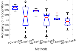
(a) Unsupervised SparLow with or without $g_{d}$

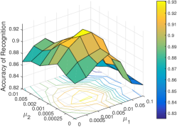
(b) PCA-SparLow

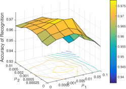
(c) LDA-SparLow

Figure 2: Impact of the regularizers to the recognition rate on the USPS digits (SparLow/R refers to PCA-SparLow methods without $g_{d}$).

6 Experimental Evaluations

In this section, we investigate performance of our proposed SparLow framework in several image processing applications. For the convenience of referencing, we adopt the following fashion to name the algorithms in comparison: for example, the PCA-like SparLow algorithm described in Section 4.1.1 is referred to as the PCA-SparLow and its sequential learning counterpart, which directly applies a PCA on the corresponding sparse representations, as SparPCA.

6.1 Experimental Settings

In unsupervised learning experiments, we employ the K-SVD algorithm [10] to compute an empirically optimal data-driven dictionary, then initialize SparLow algorithms with its column-wise normalized copy, as required by the regularizer $g_{d}$. For both supervised and semi-supervised learning, we adopt the same approach to generate a sub-dictionary for each class, and then concatenate all sub-dictionaries to form a common dictionary.

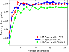
Figure 3: Trace of performance over optimization process initialized with different sparse coding methods on 15-Scenes dataset.

In order to compare the performance of the SparLow system with different initial dictionaries, Fig. 3 depicts the optimization process of LDA-SparLow performed on the 15-Scenes dataset, with the data-driven dictionary being learned by K-SVD, ODL [45] and RLS-DLR [46], respectively. Furthermore, Fig. 6 depicts the optimization process of supervised SparLow methods with the data-driven dictionary being learned by K-SVD.

With the initial dictionary $\mathbf{D}^{(0)}\in\mathfrak{S}(m,r)$ being given, the initial orthogonal projection $\mathbf{P}^{(0)}\in\mathfrak{Gr}(l,r)$ can be directly obtained by applying classic TQ maximization algorithms on the sparse representations of the samples with respect to $\mathbf{D}^{(0)}$. Certainly, when the number of training samples is huge, it is unnecessary to perform a TQ maximization in order to generate an initialization. Instead, we employ only a selection of random samples to compute the initial orthogonal projection $\mathbf{P}^{(0)}$.

In all experiments, we choose $\sigma=10^{-3}$ by hand in Eq. (12). The parameters for $\mu_{1},\mu_{2},r,l$ in Eq. (15) and $\lambda_{1},\lambda_{2}$ in Eq. (7) or $\lambda$ in KL-divergence [37] could be well tuned via performing cross validation. Images are presented as $m$-dimensional vectors, and normalized to have unit norm. For datasets without a pre-construction of training set and testing set, all experiments are repeated ten times with different randomly constructed training set and test set, and the average of per-class recognition rates is recorded for each run. For most of our experiments, we employ the elastic net method [36] to solve the sparse coding problem (6). An alternative solution based on KL-divergence is also evaluated in the application of large scale image processing in Section 6.4.

Fig. 4 plots the recognition rates of LDA-SparLow, MFA-SparLow, SRC, FDDL [19], and LC-KSVD with varying dictionary sizes (number of atoms). In all cases, the proposed methods perform better than SRC and FDDL, and give significant improvement to LC-KSVD and TDDL. This also confirms that an increasing dimension of spare representation can enhance linear separability for image classification, as observed in [29, 30].

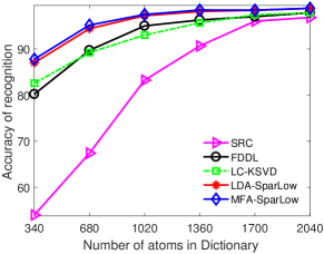
Figure 4: Comparison on recognition results with different dictionary sizes for PIE faces. The classifier is 1NN.

6.2 Tuning of Parameters

Training a SparLow model can be computationally expensive. We firstly investigate the impact of various factors of the learning model. All experiments in this subsection were conducted on the USPS dataset [47], which contains $7291$ training images and $2007$ testing images. After applying SparLow models on the images to produce the corresponding low dimensional representations, we employ the one-nearest neighbor ($1$NN) method to test the performance of the SparLow in terms of classification.

6.2.1 Weighing the Regularisers

Here, we investigate the impact of the two regularizers $g_{c}$ and $g_{d}$ on the performance of the SparLow, i.e., the inference of weighing parameters $\mu_{1}$ and $\mu_{2}$ in Eq. (15). Firstly, we test a special case that $\mu_{2}=0$, i.e., without the data regularizer. Fig. 2(a) shows the box plot of results of applying the $1$NN classification ten times on the USPS database with random initializations. As usual, the recognition accuracy is chosen as the lowest one of recognition results after the algorithm running $20$ iterations of each run, i.e., the converged value of recognition in this work. The results suggest that the regularizer $g_{d}$ has the capability of ensuring good reconstruction, and achieving stable discriminations. Fig. 6 depicts the trace of performance over optimization process of supervised SparLow on CMU PIE faces with $n_{\mathrm{train}}=120$ and USPS, respectively. All sub-figures in Fig. 6 and Fig. 2(a) show that the regularizers $g_{c}$ and $g_{d}$ can highly improve the stability of recognition accuracy after convergence.

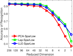
(a) Unsupervised SparLow

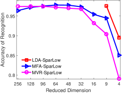
(b) Supervised SparLow

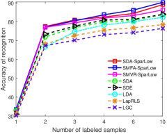
(c) Semi-supervised SparLow

Figure 5: Impact of targeted low dimensionality and number of labelled samples to the recognition rate of $1$NN classification on the USPS digits.

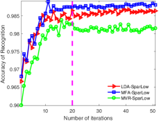
(a) PIE: with $g_{c}$ and $g_{d}$

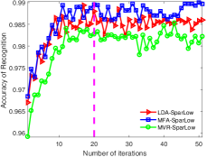
(b) PIE: without $g_{c}$ and $g_{d}$

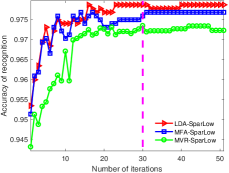
(c) USPS: with $g_{c}$ and $g_{d}$

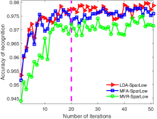
(d) USPS: without $g_{c}$ and $g_{d}$

Figure 6: Trace of performance over optimization process of supervised SparLow with or without regularizers.

We further investigate the influence of different weighing factors $\mu_{1}$ and $\mu_{2}$ for both the PCA-SparLow and LDA-SparLow on the 1NN classification problem. The experiments are performed with $r=1000$, and $l=50$ for PCA-SparLow, $l=9$ for LDA-SparLow. Fig. 2(b) and Fig. 2(c) depict the 1NN classification results of PCA-SparLow and LDA-SparLow with respect to different weighing factors $\mu_{1}$ and $\mu_{2}$. It is clear from Fig. 2(b) and Fig. 2(c) that for both PCA-SparLow and LDA-SparLow, suitable choices of $\mu_{1}$ and $\mu_{2}$ can improve the performance of the SparLow system.

6.2.2 Targeted Low Dimensionality

The main goal of this work is to learn appropriate low dimensional representations of images. In this experiment, we investigate the impact of the choice of the targeted low dimensionality $l$ to the performance of SparLow. As depicted in Fig. 5(a), SparLow models of three classic unsupervised learning algorithms are examined in terms of recognition accuracy with respect to different targeted low dimensionality $l$. It is clear that, when $l\geq 32$, all three tested unsupervised SparLow methods perform almost equally well for this specific task. Similar trends are also observed in the supervised SparLow’s as in Fig. 5(b). Hence, we conclude that, after bypassing a threshold of the targeted low dimensionality, the performance of the corresponding SparLow method is stable and reliable.

6.2.3 Number of Labelled Samples

For semi-supervised learning, one important aspect is surely the number of labelled samples. We compare the SparLow counterparts of three state of the art semi-supervised learning algorithms, i.e., SDA-SparLow versus SDA [33], SLap-SparLow versus SDE [40], SMVR-SparLow versus label propagation methods, e.g., LapRLS [42] and LGC [41].

More specifically, the dictionary $\widehat{\mathbf{D}}$ is initialized by Laplacian SparLow. For label propagation methods, e.g., LapRLS and LGC, we use the same settings as in [42, 41] for classification. We choose $\mu_{1}=2.5\times 10^{-4},\mu_{2}=5\times 10^{-3}$, $\lambda_{1}=0.2,\lambda_{2}=10^{-3}$ for all tests. Moreover, we set $\alpha=0.1$ for SDA-SparLow and SMVR-SparLow, $\alpha_{1}=0.1,\alpha_{2}=0.01$ for SMFA-SparLow. The neighborhood size is set to $20$. Our results in Fig. 5(c) show that the three semi-supervised SparLow methods consistently outperform all other state of the art methods. It is also worth noticing that with an increasing number of labeled samples, semi-supervised SparLow methods demonstrate greater advantages over their conventional counterparts.

6.3 Evaluation of Disentanglability

In this subsection, we investigate the disentanglability of the proposed SparLow framework in the setting of unsupervised learning, which is arguably to be a challenging scenario to test the ultimate goal of representation learning, i.e., to automatically disentangle underlying discriminant factors within the data. Hereby, the disentangling factors of variation could be discerned consistently across a set of images, such as the class information, various levels of illuminations, resolutions, sharpness, camera orientations, the expressions and the poses of faces, etc. In the following, we take the disentangling factors of the class information, the illuminations, the expressions and the poses of faces as examples to evaluate the disentanglability of the proposed SparLow framework.

Our first experiments are performed on the CMU-PIE face dataset [33], which consists of $68$ human subjects with $41,368$ face images in total. In our experiments, we set $\lambda_{1}=10^{-2},\lambda_{2}=10^{-5},$ $\mu_{1}=2.5\times 10^{-4},\mu_{2}=5\times 10^{-3}$. It is often considered to possess strong class information, compared to other classic recognition benchmark datasets. We follow the same experimental setting as described in [33] and choose the frontal pose and use all the images under different illuminations, so that we get $64$ images for each subject with the resized scale $32\times 32$. We compare three classic unsupervised learning methods, namely, PCA, ONPP, and OLPP, with its sequential sparsity based methods, and our proposed SparLow methods. Fig. 7 reports the performance of the three families of methods, applied to $1$NN classification problems on the CMU-PIE dataset. It is clear that the SparLow methods outperform by far the state of the art algorithms consistently.

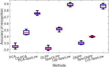
Figure 7: Face recognition on $68$ class PIE faces. The classifier is $1$NN. Randomly choose $8160$ training samples and $3394$ testing samples.

A popular intuitive approach to evaluate disentanglability of representation learning methods is via a visualization of the extracted representations. Similar to the concepts of Fisherfaces in [5], eigenfaces in [5], laplacianfaces in [4], orthogonal laplacianfaces in [32], and orthogonal LLEfaces in [2], we construct the $j^{\mathrm{th}}$ SparLow facial disentanglement $\bm{\upsilon}_{j}$ as

$$\bm{\upsilon}_{j}={\mathbf{D}}{\mathbf{u}}_{j}\in\mathbb{R}^{m},$$ (62)

with $\mathbf{u}_{j}$ being the $j^{\mathrm{th}}$ column vector of projection matrix ${\mathbf{U}}$. Fig. 8(a) shows the first ten eigenfaces, laplacianfaces, and LLEfaces from top to bottom, while Fig. 8(b) depicts the first ten basis vectors of learned disentangling factors of variation for PCA-SparLow, Lap-SparLow and LLE-SparLow, accordingly. Clearly, our learned facial features in Fig. 8(b) capture more factors of variation in faces, such as varying poses and expressions (e.g., smile), than the state of the arts in Fig. 8(a).

(1)

(2)

(3)

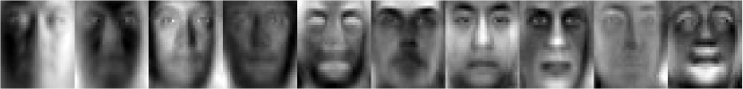
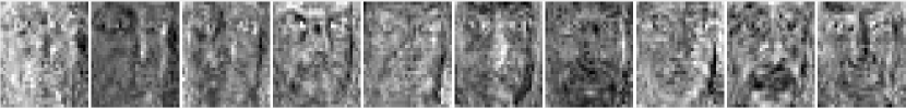
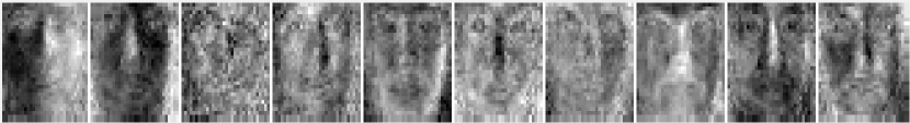
(a) Features extracted from original data

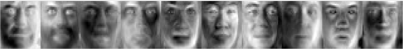
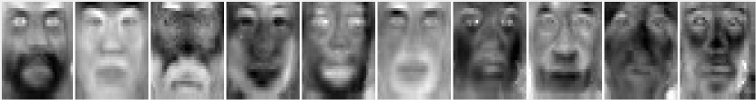
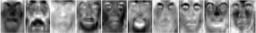
(b) Features extracted from sparse representations

Figure 8: Visualisation of facial features on PIE faces [33]. The presented features are generated via Eq. (62). From top to bottom: (1) PCA eigenfaces; (2) Laplacianfaces; (3) LLEfaces.

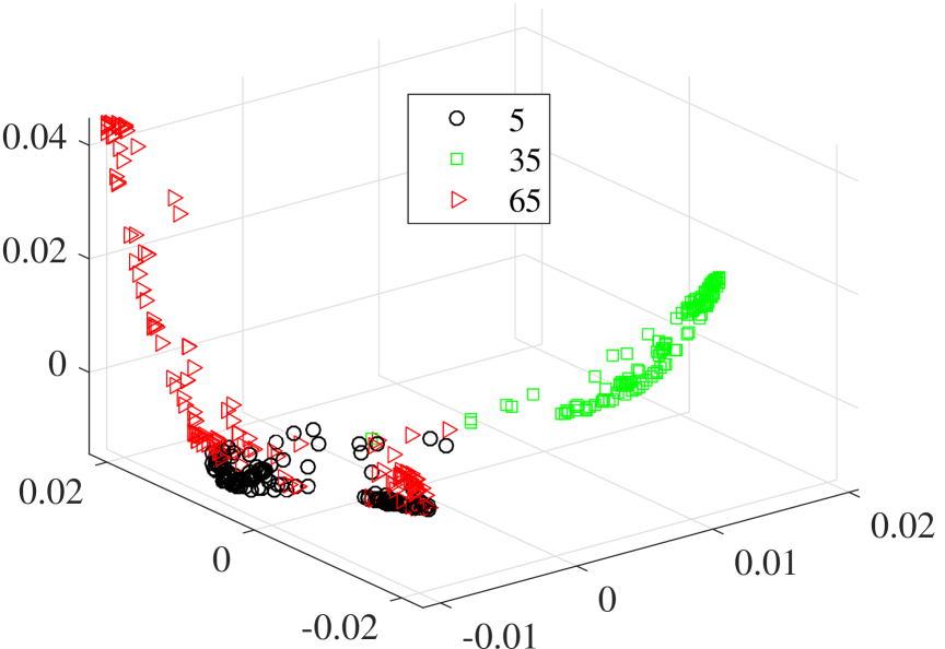
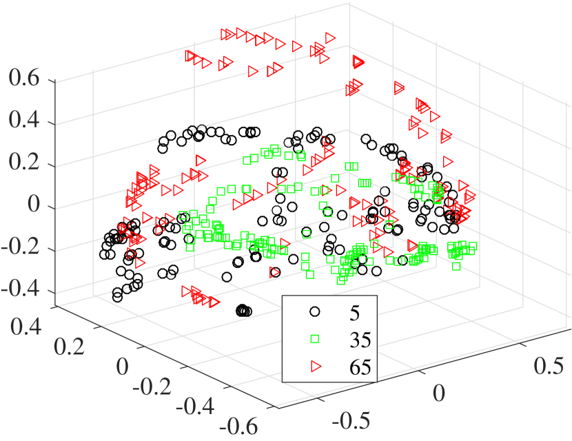
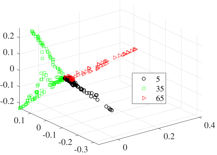
(a) OLPP Family

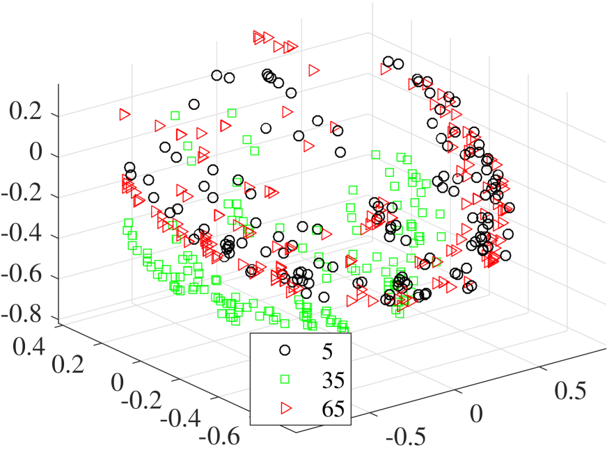
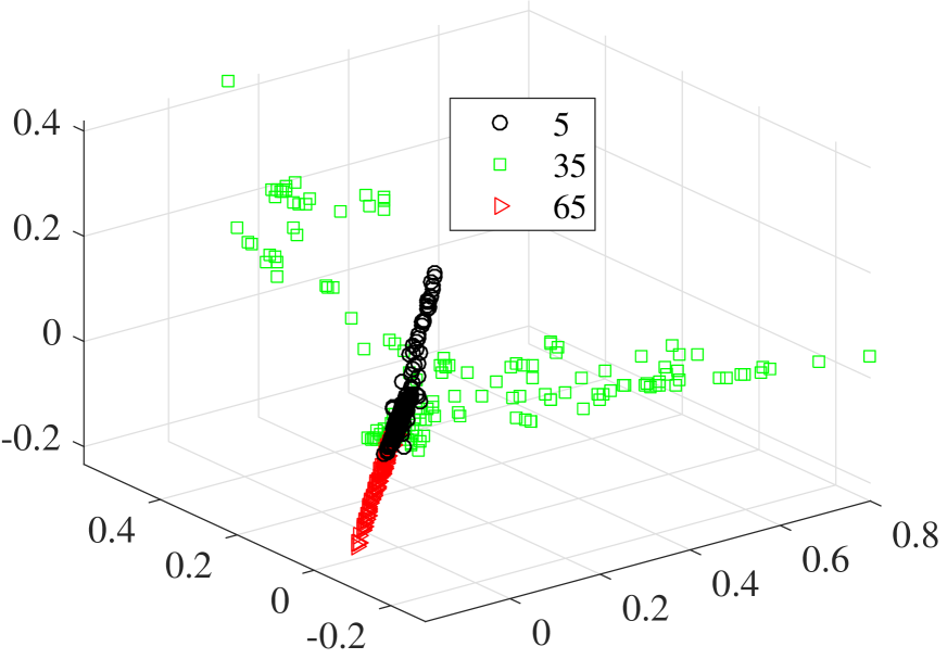
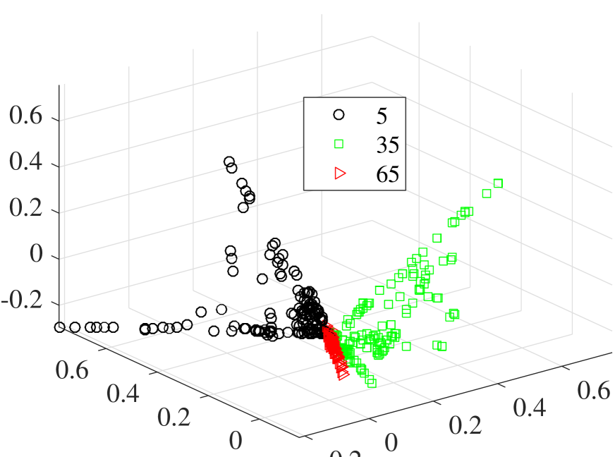
(b) PCA Family

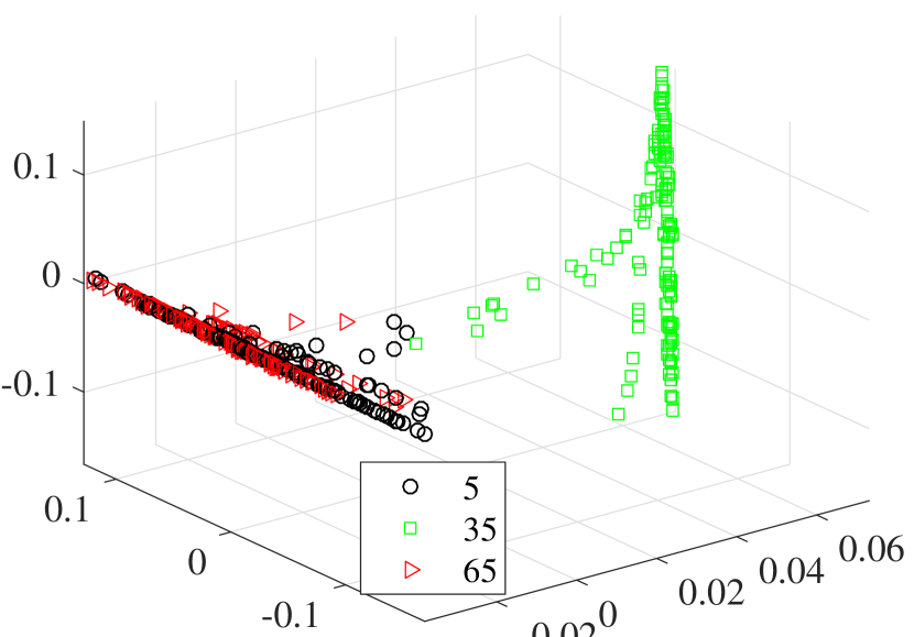
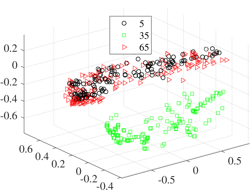
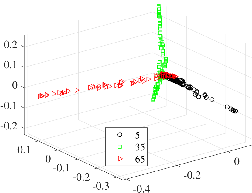
(c) ONPP Family

Figure 9: 3D visualisation of PIE faces (class 5, 35, 65). From top to bottom: Applying OLPP/PCA/ONPP in original space, in sparse space with respect to initial dictionary $\widehat{\mathbf{D}}$, and in sparse space with respect to learned dictionary via SparLow, respectively.

Furthermore, we aim to intuitively illustrate the disentangled factor by visualizing the low dimensional image representations, i.e., $3D$. As suggested in [33], a subset containing $11,554$ PIE faces with five near frontal poses (C05, C07, C09, C27, C29) and different illuminations are chosen, thus we nearly get $170$ images for each individual. Our experiments of 3D visualization were conducted on PIE faces (class 5, 35, 65), compared to their classic counterparts. As depicted in Fig. 9, the $3D$ representations captured in the original data space, shown in the first row in Fig. 9, are hardly possible to cluster or group. In particular, the boundary between each pair of faces are completely entangled. It is evidential that visualization powered by the SparLow, i.e., the third row in Fig. 9, leads to direct clustering of the faces. In short, the class information is clearly disentangled, while the other approaches fail.

Then we perform 3D visualization on PIE faces without class information. We choose $70$ faces from the class $5$ with $2$ factors of variations, i.e., poses and illuminations. As can be seen from the Fig. 10, the information referred to poses and illuminations could be clearly disentangled. In Fig. 10(a), from left to right, the illumination become stronger. From top to bottom, the poses of faces change from left to right. The similar results are also shown in Fig. 10(b) and Fig. 10(c).

(a) PCA-SparLow.

(b) OLPP-SparLow

(c) ONPP-SparLow

Figure 10: 2D visualization of PIE faces (class 5).

Our last experiments in this subsection are performed on handwritten digits, i.e., the MNIST dataset and the USPS dataset. The MNIST dataset consists of $60000$ handwritten digits images for training and $10000$ digits images for testing. The parameters for elastic net are set to be $\lambda_{1}=0.2$, $\lambda_{2}=2\times 10^{-5}$, and $\mu_{1}=5\times 10^{-3}$, $\mu_{2}=4\times 10^{-4}$, for both experiments on the MNIST and USPS datasets. We compare the SparLow methods to several state of the art methods, on the task of $1$NN and Gaussian SVM (GSVM) classification. For PCA, KPCA and PCA-SparLow, we set $l=50$, for other methods, we set $l=20$. For USPS, we use the full training and testing dataset. For MNIST, we randomly choose $30000$ images for training, and use standard $10000$ testing dataset. Our results in Table I suggest that the SparLow methods consistently outperform the state of the arts.

Methods	USPS (1NN)	USPS (GSVM)	MNIST (1NN)	MNIST (GSVM)
PCA [27]	$86.40\%$, $l=50$	$92.43\%$, $l=50$	$84.62\%$, $l=50$	$94.63\%$, $l=50$
Sparse PCA [48]	$87.66\%$	$88.91\%$	$86.10\%$	$90.88\%$
OLPP [32]	$84.11\%$	$91.48\%$	$83.12\%$	$94.76\%$
ONPP [31]	$87.39\%$	$92.73\%$	$85.01\%$	$95.21\%$
KPCA [31]	$89.19\%$, $l=50$	$93.27\%$, $l=50$	$-$	$-$
LLE [2]	$68.81\%$	$90.43\%$	$66.09\%$	$93.11\%$
LE [31]	$71.85\%$	$91.93\%$	$68.16\%$	$93.90\%$
ISOMAP [31]	$64.80\%$	$90.13\%$	$60.51\%$	$91.67\%$
CS-PCA [27]	$87.84\%$	$94.22\%$	$87.65\%$	$96.04\%$
PCA-SparLow	$92.18\%$, $l=50$	$96.82\%$, $l=50$	$91.23\%$, $l=50$	$97.12\%$
Lap-SparLow	$91.83\%$	$96.26\%$	$89.32\%$	$96.91\%$
LLE-SparLow	$90.78\%$	$96.16\%$	$89.10\%$	$96.93\%$

TABLE I: Classification Performance (Accuracy (%)) for the MNIST & USPS datasets of the Proposed SparLow methods, with comparisons to some classical unsupervised approaches.

6.4 Performance in Large Scale Image Processing

Finally, we investigate performance of the SparLow model in large scale image processing applications, specifically, the problem of object categorization on large scale image dataset with complex backgrounds, such as the images from Caltech-101 [49], Caltech-256 [50] and 15-Scenes [51].

TABLE II: Classification Performance (Average accuracy (%)) on Caltech-101 & Caltech-256 datasets.

(a) Caltech-101	1	5	10	15	20	25	30	(b) Caltech-256	15	30	45	60
KSPM [51]	$-$	$-$	$-$	$56.40$	$-$	$-$	$64.40$	KSPM [51]	$-$	$34.10$	$-$	$-$
ScSPM+SVM [16]	$-$	$-$	$-$	$67.0$	$-$	$-$	${73.2}$	ScSPM+SVM [16]	$27.73$	$34.02$	$37.46$	$40.14$
LLC+SVM [17]	$-$	$51.15$	$59.77$	$65.43$	$67.74$	$70.16$	${73.44}$	LLC+SVM [17]	$34.36$	$41.19$	$45.31$	$47.68$
Griffin [50]	$-$	$44.2$	$54.5$	$59.0$	$63.3$	$65.8$	$67.60$	Griffin [50]	$28.30$	$34.10$	$-$	$-$
SRC [13, 22]	$-$	$48.8$	$60.1$	$64.9$	$67.5$	$69.2$	$70.7$	SRC [13, 22]	$27.86$	$33.33$	$-$	$-$
D-K-SVD [21, 22]	$-$	$49.6$	$59.5$	$65.1$	$68.6$	$71.1$	${73.0}$	D-K-SVD [21, 22]	$-$	$33.72$	$-$	$48.88$
BMDDL [23]	$31.88$	$56.10$	$66.01$	$69.56$	$71.32$	$72.28$	${75.54}$	BMDDL[23]	$35.41$	$41.56$	$46.90$	$52.32$
LC-K-SVD [22]	$28.9$	$54.0$	$63.1$	$67.7$	$70.5$	$72.3$	${73.6}$	LC-K-SVD [22]	$28.9$	$34.32$	$-$	$-$
FDDL [19]	$-$	$51.1$	$60.6$	$65.6$	$68.5$	$70.4$	$71.0$	FDDL [19]	$-$	$-$	$-$	$-$
SSPIC [15]	$-$	$55.1$	$62.1$	$65.0$	$67.5$	$68.9$	$71.5$	LSc [14]	$29.99$	$35.74$	$38.47$	$40.32$
LDA+GSVM	$-$	$50.49$	$60.39$	$64.28$	$67.10$	$71.24$	$72.40$	TDDL [24]	$33.14$	$39.05$	$44.16$	$49.05$
SparLDA	$-$	$54.60$	$65.26$	$70.05$	$72.12$	$73.2$	$75.82$	SparLDA	$35.62$	$39.53$	$47.08$	$51.90$
LDA-SparLow	$31.23$	$56.44$	$67.12$	$73.82$	$74.70$	$76.20$	$76.86$	LDA-SparLow	$38.05$	$43.26$	$50.32$	$55.74$
SDA-SparLow	$46.12$	$67.42$	$72.01$	$76.12$	$76.64$	$77.40$	$78.25$	SparMFA	$36.42$	$40.89$	$47.62$	$51.76$
MFA-SparLow	$32.43$	$57.52$	$68.44$	$73.95$	$75.56$	$76.63$	$77.32$	MFA-SparLow	$38.82$	$44.05$	$51.34$	$56.82$
SMFA-SparLow	$46.02$	$68.66$	$72.92$	$76.02$	$77.24$	$77.80$	$78.42$	SparMVR	$32.90$	$37.91$	$45.03$	$50.64$
MVR-SparLow	$29.30$	$54.79$	$65.63$	$70.56$	$73.33$	$75.41$	$76.15$	MVR-SparLow	$36.29$	$40.66$	$47.92$	$52.56$
SMVR-SparLow	$44.82$	$66.43$	$70.80$	$75.48$	$76.32$	$77.14$	$77.76$		$-$	$-$	$-$	$-$

We adopt a popular approach of object categorization to firstly detect certain local image features, such as dense SIFT or dense DHOG (a fast SIFT implementation) [52], then to quantize them into discrete “visual words” over a codebook, and finally to compute a fixed-length Spatial Pyramid Pooling (SPP) vector of acquired “visual words” [16, 17, 51]. We refer to such an approach as the SIFT/DHOG-SPP representation. In our experiments, the local descriptor is extracted from $s\times s$ pixel patches densely sampled from each image, specifically, we choose $s=16$ for SIFT and $s=16,25,31$ for DHOG. The dimension of each SIFT/DHOG descriptor is $128$. A codebook with the size of $k=1024$ or $k=2048$, is learned for coding SIFT/DHOG descriptors. We then divide the image into $4\times 4$, $3\times 3$ and $1\times 1$ subregions, i.e., $21$ bins. The spatial pooling procedure for each spatial sub-region is applied via the max pooling function associated with an “$\ell_{2}$ normalisation”, e.g., [16, 17, 22, 25]. The final SPP representations are computed with the size $m=21504$ or $m=43008$, and hence are reduced into a low-dimensional PCA-projected subspace. In what follows, we denote by $m,m_{\mathrm{PCA}},r,l$ the dimension of SPP representation, PCA projected subspace, sparse codes, and learned low dimensional representation, respectively.

6.4.1 Number of Reduced Features

It is known that the computational complexity of sparse coding mainly depends on the choice of dictionary size [35]. It is hence necessary to investigate the impact of the number of features to the performance of SparLow. We employ a popular approach to firstly apply a classic PCA transformation on the SPP features, and then learn a dictionary on reduced features [13]. In this experiment, we deploy the Caltech-101 dataset [49], which contains $9144$ images from $102$ classes. Most images are in medium resolution (about $300\times 300$ pixels). Fig. 11 show the recognition results of several supervised SparLow and semi-supervised SparLow methods with PCA projected SPP features. It is obvious that after reaching a certain number of reduced features, i.e., $l>1024$, all methods in test show no significant improvement. Moreover, it is worth knowing that the performance of two semi-supervised SparLow methods consistently outperform other methods.

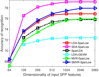
Figure 11: Recognition results using proposed MFA-SparLow in PCA projected subspace on Caltech-101 dataset. $n_{\mathrm{train}}=30$, $r=3060$.

6.4.2 Caltech-101 dataset

Learning on Caltech-101 dataset is often considered to be hard, since the number of images per category varies significantly from $31$ to $800$. In our experiments, we set $\lambda_{1}=5\times 10^{-2},\lambda_{2}=10^{-5}$, $k=1024$, $r=1020$, and choose $l\in\{101,287,512\}$ are set for LDA, MFA, MVR related methods, respectively. We confine ourselves to the same experimental settings as used in [16, 17, 51]. We randomly select $1$, $5$, $10$, $15$, $20$ and $30$ labeled images per category for training and the rest images for testing. For semi-supervised SparLow, the training set includes all labeled and unlabelled images. Table II (a) gives a comparison of LDA-SparLow, SLDA-SparLow with approaches from the literatures. Note that, for the number of labeled samples $n_{l}=1$, LDA and LDA-SparLow are not applicable. It shows that our proposed approaches consistently outperform all the competing approaches. Especially, the semi-supervised SparLow could significantly improve the recognition accuracy when the labeled training samples are limit. The possible reason is that some categories have large samples, e.g., the category airplanes has $800$ samples, the $n_{l}\leq 30$ is too much limit for training such a category. Semi-supervised SparLow’s take advantage of all the data for training sparsifying dictionary, which is the key factor to promote the discrimination of sparse representations.

6.4.3 Caltech-256 dataset

The Caltech-256 dataset consists of $30607$ images from $256$ categories with various resolutions from $113\times 150$ to $960\times 1280$. Each category has at least $80$ images. Unlike the Caltech-$101$ dataset, this dataset contains multiple objects in various poses at different locations within the images. Existence of background clutter and occlusion result in higher intraclass diversity, which makes the categorization task even harder.

We apply our DHOG-SPP SparLow on randomly selected $15$, $30$, $45$, $60$ training images per category, respectively. We set $\lambda=0.1$, $m_{\mathrm{PCA}}=2560$, $k=2048$, $r=3128$. For LDA-like SparLow, MFA-like SparLow and MVR-like SparLow, we set $l=255$, $361$ and $387$, respectively. Finally, we use GSVM for classifying the low dimensional representations. In this experiment, we use the sparse coding formulation associated with KL-divergence. Table II (b) shows that our results outperform the state of the art methods under all the cases. Moreover, we also implemented TDDL for comparison, and the each sub-dictionary size of TDDL is fixed as $r=200$. It shows that TDDL’s perform worse than the SparLow’s. The possible reason is that TDDL’s associated with a binary classifier may suffer the huge number of classes.

6.4.4 15-Scenes dataset

We finally evaluate the SparLow framework on the 15-Scenes dataset [51]. This dataset contains totally $4485$ images falling into $15$ categories, with the number of images in each category ranging from $200$ to $400$ and image size around $300\times 250$ pixels. The image content is diverse, containing not only indoor scenes, such as bedroom, kitchen, but also outdoor scenes, such as building and country views, etc.

Following the common experimental settings, we use SIFT-SPP as input with $k=1024$ and $m_{\mathrm{PCA}}=2000$. For MFA, we set $k_{1}=70,k_{2}=100$, and $l=50$. For SparMFA and MFA-SparLow, we set $k_{1}=30,k_{2}=100$ and $l=60$. For all supervised and semi-supervised SparLow methods, the dictionary size $r=750$. Table III compares our results with several sparse coding methods in [16, 13, 17, 14, 21, 22, 23, 53], GSVM, and the method in [51], which are all using SPP features as input data. As shown in Table III, our approaches significantly outperform all state of the art approaches. Note that, the bottom three lines are all semi-supervised methods.

Methods	Accuracy	Methods	Accuracy
BMDDL [23]	$96.9$	Lobel [53]	$86.3\pm 0.5$
GSVM	$72.2$	LDA	$91.69$
KSPM [51]	$83.50$	SparLDA	$95.89$
ScSPM+GSVM [16]	$80.28$	LDA-SparLow	$97.47$
LLC+GSVM [17]	$89.2$	MFA	$92.82$
SRC [13, 22]	$91.8$	SparMFA	$96.65$
LSc [14]	$89.7$	MFA-SparLow	$98.46$
K-SVD[10] + LDA	$92.6$	MVR ($l=512$)	$93.10$
D-K-SVD [21]	$89.01$	SparMVR	$96.32$
LC-K-SVD [22]	$92.9$	MVR-SparLow	$97.55$
FDDL [19]	$90.2$	$-$	$-$
SDA [33]	$97.28$	SDA-SparLow	$99.18$
SDE [40]	$97.66$	SLap-SparLow	$99.25$
LapRLS [42]	$94.86$	SMVR-SparLow	$99.12$

TABLE III: Averaged classification Rate (%) comparison on 15-Scenes dataset. The classifier is $1$NN for the third column if not specified.

7 Conclusion

In this work, we present a low dimensional representation learning approach, coined as SparLow, which leverages both sparse representation and the trace quotient criterion. It can be considered as a two-layer disentangling mechanism, which applies the trace quotient criterion on the sparse representations. Our proposed generic cost function is defined on a sparsifying dictionary and an orthogonal transformation, which form a product Riemannian manifold. A geometric CG algorithm is developed for optimizing the SparLow function. Our experimental results depict that in comparison with the state of the art unsupervised, supervised and semi-supervised representation learnings methods, our proposed SparLow framework delivers promising performance in data visualization and classification. Moreover, the proposed SparLow is flexible and can be extended to more general cases of low dimensional representation learning models with orthogonal constraints.

Xian Wei (S’14-M’18) received the Ph.D. degree in Engineering from the Technical University of Munich, Munich, Germany, in 2017. In July 2017, he joined Fujian Institute of Research on the Structure of Matter, Chinese Academy of Sciences, China, as a leading Researcher of Machine Vision and Pattern Recognition Lab. His research interests focus on sparse coding, deep learning and geometric optimization. The applications include robotic vision, videos or images modeling, synthesis, recognition and semantics.

Hao Shen (S’04-M’08) received his PhD in Engineering from the Australian National University, Australia, in 2008. From December 2008 to September 2017, he was a post-doctoral researcher at the Institute for Data Processing, Technische Universität München, Germany. In October 2017, he joined fortiss, State Research institute of Bavaria, Germany, as the leader of Machine Learning Lab. His research interests focus on machine learning for signal processing, e.g., deep representation learning, and reinforcement learning.

Martin Kleinsteuber received his Ph.D. in Mathematics from the University of Würzburg, Germany, in 2006. After post-doc positions at National ICT Australia Ltd., the Australian National University, Canberra, Australia, and the University of Würzburg, he has been appointed assistant professor for geometric optimization and machine learning at the Department of Electrical and Computer Engineering, TU München, Germany, in 2009. Since 2016, he is leading the Data Science Group at Mercateo AG, Munich.

Appendix A Proof of Proposition 1

Note, that the numbering of equations in Appendix continues from the numeration in the manuscript. The proof of Proposition 1 requires the following two lemmas.

Lemma 1.

Let $g\colon\mathbb{R}^{r}\to\mathbb{R}$ satisfy Assumption 1. Then, for a given $\mathbf{x}\in\mathbb{R}^{m}$ and a dictionary $\mathbf{D}\in\mathbb{R}^{m\times r}$, a vector $\boldsymbol{\phi}^{*}:=[\varphi_{1}^{*},\ldots,\varphi_{r}^{*}]^{\top}\in\mathbb{R}^{r}$ is the unique solution to the sparse regression problem as in Eq. (5), if and only if, the following conditions hold

$$\left\{\!\!\begin{array}[]{ll}\mathbf{d}_{i}^{\top}(\mathbf{x}-\mathbf{D}\boldsymbol{\phi}^{*})=\nabla g_{i}(\varphi_{i}^{*}),&\quad~{}\text{for}~{}\varphi_{i}\neq 0,\\[1.42262pt] \mathbf{d}_{i}^{\top}(\mathbf{x}-\mathbf{D}\boldsymbol{\phi}^{*})\in\partial g_{i}(0),&\quad~{}\text{for}~{}\varphi_{i}=0.\end{array}\right.$$ (63)

Here $\partial g_{i}(0)=[-b_{1},b_{2}]$ with $b_{1},b_{2}>0$ is the subgradient of element-wise regulariser $g_{i}$ at $0$.

Proof.

Since the cost function Eq. (5) is strictly convex as a result of $g$ being strictly convex, the unique solution $\boldsymbol{\phi}^{*}$ satisfies the subdifferential optimality condition, i.e.,

$$0\in\partial f_{s}(\boldsymbol{\phi}^{*}),$$ (64)

where $\partial f_{s}(\boldsymbol{\phi}^{*})$ is the subdifferential of $f_{s}$ at $\boldsymbol{\phi}^{*}$. By the construction that the cost function is separable, the subdifferential of the cost function is computed as

$$\mathbf{d}_{i}^{\top}(\mathbf{x}-\mathbf{D}\boldsymbol{\phi}^{*})\in\partial g_{i}(\varphi_{i}).$$ (65)

By the fact that $\partial g_{i}(\varphi_{i})=\nabla_{\!g_{i}\!}(\varphi_{i})$ for all $\varphi_{i}^{*}\neq 0$, the result follows. ∎

Lemma 2.

Let $g\colon\mathbb{R}^{r}\to\mathbb{R}$ satisfy Assumption 1, and Assumption 2 hold true. Then, for a given $\mathbf{x}\in\mathbb{R}^{m}$ and a dictionary $\mathbf{D}\in\mathbb{R}^{m\times r}$, the unique solution $\boldsymbol{\phi}^{*}:=[\varphi_{1}^{*},\ldots,\varphi_{r}^{*}]^{\top}\in\mathbb{R}^{r}$ to the sparse regression problem as in Eq. (5) is smooth in an open neighborhood around $\mathbf{D}^{*}$.

Proof.

Recall the definition of support $\mathfrak{P}(\mathbf{x},\mathbf{D}^{*})$ as in Eq. (42), we define its complement set as

$$\mathfrak{Q}(\mathbf{x},\mathbf{D}^{*}):=\{i\in\{1,\ldots,r\}|\varphi^{*}_{i}=0\}.$$ (66)

Let $k=|\mathfrak{P}(\mathbf{x},\mathbf{D})|$, $\boldsymbol{\phi}_{\mathfrak{P}}\in\mathbb{R}^{k}$ and $\mathbf{D}_{\mathfrak{P}}\in\mathbb{R}^{m\times k}$ being the subset of $\mathbf{D}\in\mathbb{R}^{m\times r}$, in which the indices of columns fall into the support $\mathfrak{P}$. We construct a function as

$$\begin{split}\eta&\colon\mathbb{R}^{m\times r}\times\mathbb{R}^{r}\to\mathbb{R}^{r},\\[-2.84526pt] \eta&(\mathbf{D},\boldsymbol{\phi}):=\mathbf{D}_{[\mathfrak{P},\mathfrak{Q}]}^{\top}(\mathbf{x}-\mathbf{D}_{[\mathfrak{P},\mathfrak{Q}]}\boldsymbol{\phi})-\begin{bmatrix}\nabla g_{\mathfrak{P}}(\boldsymbol{\phi}_{\mathfrak{P}})\\ \boldsymbol{\phi}_{\mathfrak{Q}}\end{bmatrix},\\[-2.84526pt] \end{split}$$ (67)

with $\boldsymbol{\phi}=[\boldsymbol{\phi}_{\mathfrak{P}}^{\top}~{}\boldsymbol{\phi}_{\mathfrak{Q}}^{\top}]^{\top}$, $\boldsymbol{\phi}_{\mathfrak{P}}\in\mathbb{R}^{k}$, and $\boldsymbol{\phi}_{\mathfrak{Q}}\in\mathbb{R}^{r-k}$. The function $\eta$ is smooth in both $\mathbf{D}$ and $\boldsymbol{\phi}$, and $\eta(\mathbf{D}^{*},\boldsymbol{\phi}^{*})=0$. Taking the directional derivative of $\eta$ with respect to $\mathbf{D}$ and $\boldsymbol{\phi}$ leads to

$$\begin{split}&\operatorname{D}\eta(\mathbf{D},\boldsymbol{\phi})(\mathbf{H}_{\mathbf{D}},\mathbf{h}_{\boldsymbol{\phi}})\\[-2.84526pt] =&\underbrace{\begin{bmatrix}\chi_{1}(\mathbf{D}_{[\mathfrak{P},\mathfrak{Q}]},\boldsymbol{\phi})&\!\!\chi_{2}(\mathbf{D}_{[\mathfrak{P},\mathfrak{Q}]},\boldsymbol{\phi})\end{bmatrix}}_{=:J_{\eta}(\mathbf{D},\boldsymbol{\phi})\in\mathbb{R}^{r\times(r+m\cdot r)}}\cdot\begin{bmatrix}\mathbf{h}_{\phi}\\ \operatorname{vec}(\mathbf{H}_{\mathbf{D}})\end{bmatrix},\\[-2.84526pt] \end{split}$$ (68)

where

$$\chi_{1}(\mathbf{D}_{[\mathfrak{P},\mathfrak{Q}]},\boldsymbol{\phi})\!:=\!\begin{bmatrix}\mathsf{H}g_{\mathfrak{P}}(\boldsymbol{\phi}_{\mathfrak{P}})\!&\!\mathbf{0}_{k,r-k}\\ \mathbf{0}_{r-k,k}\!&\!\mathbf{I}_{r-k}\end{bmatrix}\!+\!\mathbf{D}_{[\mathfrak{P},\mathfrak{Q}]}^{\top}\mathbf{D}_{[\mathfrak{P},\mathfrak{Q}]},$$ (69)

and $\chi_{2}(\mathbf{D}_{[\mathfrak{P},\mathfrak{Q}]},\boldsymbol{\phi})\in\mathbb{R}^{r\times(m\cdot r)}$ is a tedious term without clear knowledge on its rank. Here, $\mathsf{H}g_{\mathfrak{P}}(\boldsymbol{\phi}_{\mathfrak{P}})\in\mathbb{R}^{k\times k}$ is the Hessian matrix of the separable sparsifying function restricted on the support $\mathfrak{P}$, i.e., $g_{\mathfrak{P}}:=\{g_{i}\}\in\mathbb{R}^{k}$ with $i\in\mathfrak{P}$. The matrix $J_{\eta}(\mathbf{D},\boldsymbol{\phi})$ is known as the Jacobian matrix of $\eta$. Our aim is to ensure the full rankness of the Jacobian matrix to apply the implicit function theorem [1]. Often, it is assumed that $m\leq r$. Let $\kappa(\mathbf{D})$ be the spark of $\mathbf{D}$, i.e., the smallest number of columns from $\mathbf{D}$ that are linearly dependent [2]. If $k<\kappa(\mathbf{D})$, then the Jacobian matrix $J_{\eta}(\mathbf{D},\boldsymbol{\phi})$ is of full rank. Unfortunately, the spark is often very difficult to control during an optimization procedure. Thus, a simple but general fix to make $J_{\eta}(\mathbf{D},\boldsymbol{\phi})$ have full rank is to have Hessian $\mathsf{H}g_{\mathfrak{P}}(\boldsymbol{\phi}_{\mathfrak{P}})$ non-degenerate. In other words, by Assumption 2 and the implicit function theorem, there exist two open neighborhood containing $\mathbf{D}^{*}$ and $\boldsymbol{\phi}^{*}$, i.e., $\mathbf{D}^{*}\in\mathfrak{U}$ and $\boldsymbol{\phi}^{*}\in\mathfrak{W}$, and a unique continuously differentiable function $\widehat{\boldsymbol{\phi}}\colon\mathfrak{U}\to\mathfrak{W}$, so that $\widehat{\boldsymbol{\phi}}(\mathbf{D}^{*})=\boldsymbol{\phi}^{*}$ and $\eta(\mathbf{D},\widehat{\boldsymbol{\phi}}(\mathbf{D}))=0$ for all $(\mathbf{D},\boldsymbol{\phi})\in\mathfrak{U}\times\mathfrak{W}$.

Let us denote $\widehat{\boldsymbol{\phi}}(\mathbf{D}):=[\widehat{\varphi}_{1}(\mathbf{D}),\ldots,\widehat{\varphi}_{r}(\mathbf{D})]^{\top}\in\mathbb{R}^{r}$. Since $\widehat{\boldsymbol{\phi}}$ is continuously differentiable in $\mathbf{D}$ and $\widehat{\boldsymbol{\phi}}(\mathbf{D}^{*})=\boldsymbol{\phi}^{*}$, there exists an open subset $\mathfrak{U}_{\epsilon}\subset\mathfrak{U}$, so that the following holds true with a gap $\epsilon>0$ and $\epsilon<\min\{b_{1},b_{2}\}$

$$\left\{\!\!\begin{array}[]{ll}|\widehat{\varphi}_{i}(\mathbf{D})-\varphi_{i}^{*}|<\epsilon,&\text{~{}for~{}}i\in\mathfrak{P};\\[1.42262pt] |\widehat{\varphi}_{i}(\mathbf{D})|<\epsilon,&\text{~{}for~{}}i\notin\mathfrak{P}.\end{array}\right.$$ (70)

We then construct the following projection

$$\Pi_{\mathfrak{P}}\colon\mathbb{R}^{r}\to\mathbb{R}^{r},\qquad\boldsymbol{\phi}\mapsto\widetilde{\boldsymbol{\phi}}:=[\widetilde{\varphi}_{1},\ldots,\widetilde{\varphi}_{r}]^{\top},\vspace{-1mm}$$ (71)

where

$$\widetilde{\varphi}_{i}:=\left\{\begin{array}[]{ll}\varphi_{i},&\text{~{}for~{}}\varphi_{i}\notin\partial g_{i}(0);\\[1.42262pt] 0,&\text{~{}for~{}}\varphi_{i}\in\partial g_{i}(0).\end{array}\right.$$ (72)

It is clear that the projection $\Pi_{\mathfrak{P}}$ does not change support, and is hence smooth in $\boldsymbol{\phi}$. Consequently, the composition $\Pi_{\mathfrak{P}}(\widehat{\boldsymbol{\phi}}(\mathbf{D}))$ is a smooth function in $\mathbf{D}$, and is the unique solution of the sparse regression problem for given $(\mathbf{D},\mathbf{x})$ with $\mathbf{D}\in\mathfrak{U}_{\epsilon}$ by Lemma 1, i.e., $\Pi_{\mathfrak{P}}(\widehat{\boldsymbol{\phi}}(\mathbf{D}))=\boldsymbol{\phi}^{*}(\mathbf{D})$. Thus, the result follows. ∎

Finally, the proof of Proposition 1 is straightforward.

Proof.

For each sample $\mathbf{x}_{i}$ with $i=1,\ldots,n$, let us denote by $\boldsymbol{\phi}_{i}^{*}$ the sparse representation with respect to a common dictionary $\mathbf{D}^{*}$. We further denote by $\mathfrak{U}_{\epsilon_{i}}$ an open neighborhood containing $\mathbf{D}^{*}$, so that the unique solution $\boldsymbol{\phi}_{i}^{*}(\mathbf{D})$ is smooth. Then a finite number of unions of sets $\mathfrak{U}_{\epsilon_{i}}$ is a non-empty set as

$$\mathfrak{U}_{\epsilon^{*}}:=\bigcap_{i=1}^{n}\mathfrak{U}_{\epsilon_{i}}$$ (73)

with $\epsilon^{*}:=\min_{i}\epsilon_{i}$. It is straightforward to conclude that the complete collection of $\boldsymbol{\Phi}^{*}=[\boldsymbol{\phi}_{1}^{*},\ldots,\boldsymbol{\phi}_{n}^{*}]$ is smooth in $\mathfrak{U}_{\epsilon^{*}}$. ∎

In the rest of this appendix, we show a lemma, which enables development of gradient based algorithms.

Proposition 2.

Let $g\colon\mathbb{R}^{r}\to\mathbb{R}$ satisfy Assumption 1, and for a given $\mathbf{x}\in\mathbb{R}^{m}$ and a dictionary $\mathbf{D}^{*}\in\mathbb{R}^{m\times r}$, let $\boldsymbol{\phi}^{*}\in\mathbb{R}^{r}$ be the unique solution to the sparse regression problem as in Eq. (5). Then, the first derivative of $\boldsymbol{\phi}_{\mathfrak{P}}^{*}$ has a close form expression as

$$\operatorname{D}\!\phi_{\mathfrak{P}}^{*}(\mathbf{D}_{\mathfrak{P}})\mathbf{H}=\!\big{(}K(\mathbf{D}_{\mathfrak{P}})\big{)}^{\!\!\!{}^{-1}}\!\!\Big{(}\!\mathbf{H}^{\top}\!\mathbf{x}\!-\!\big{(}\mathbf{H}^{\!\top}\!\mathbf{D}_{\mathfrak{P}}\!+\!\mathbf{D}_{\mathfrak{P}}^{\top}\mathbf{H}\big{)}\boldsymbol{\phi}_{\mathfrak{P}}^{*}\!\Big{)}.\!$$ (74)

Proof.

Recall the results from Lemma 2, the unique solution $\boldsymbol{\phi}^{*}=[\varphi_{1}^{*},\ldots,\varphi_{r}^{*}]^{\top}\in\mathbb{R}^{r}$ is smooth in an open neighborhood around $\mathbf{D}^{*}$. Since the support $\mathfrak{P}(\mathbf{x}_{i},\mathbf{D}^{*})$ stays unchanged, the vector $\boldsymbol{\phi}_{\mathfrak{P}}$ is smooth in an appropriate open neighborhood containing $\mathbf{D}_{\mathfrak{P}}$, i.e., we can compute

$$\nabla_{g_{\mathfrak{P}}}(\boldsymbol{\phi}_{\mathfrak{P}})=\mathbf{D}_{\mathfrak{P}}^{\top}(\mathbf{x}-\mathbf{D}_{\mathfrak{P}}\boldsymbol{\phi}_{\mathfrak{P}}).$$ (75)

We then take the derivative on the both sides of Eq. (75) with respect to $\mathbf{D}_{\mathfrak{P}}$ in direction $\mathbf{H}\in T_{\mathbf{D}_{\mathfrak{P}}}\mathfrak{S}(m,k)$ as

$$\begin{split}\!\!\!\operatorname{D}\!\left(\nabla_{\!g_{\mathfrak{P}}}(\boldsymbol{\phi}_{\mathfrak{P}}(\mathbf{D}_{\mathfrak{P}}))\right)\!\mathbf{H}=\,&\mathbf{H}^{\top}\!(\mathbf{x}-\mathbf{D}_{\mathfrak{P}}\boldsymbol{\phi}_{\mathfrak{P}})\!-\!\mathbf{D}_{\mathfrak{P}}^{\top}\mathbf{H}\boldsymbol{\phi}_{\mathfrak{P}}\\ &\!-\!\mathbf{D}_{\mathfrak{P}}^{\top}\mathbf{D}_{\mathfrak{P}}\operatorname{D}\boldsymbol{\phi}_{\mathfrak{P}}(\mathbf{D}_{\mathfrak{P}})\mathbf{H}.\end{split}$$ (76)

The left hand side in Eq. (76) can be computed by

$$\operatorname{D}\!\left(\nabla_{\!g_{\mathfrak{P}}}(\boldsymbol{\phi}(\mathbf{D}))\right)\!\mathbf{H}=\mathsf{H}g_{\mathfrak{P}}(\boldsymbol{\phi}_{\mathfrak{P}})\cdot\operatorname{D}\boldsymbol{\phi}_{\mathfrak{P}}(\mathbf{D}_{\mathfrak{P}})\mathbf{H},$$ (77)

where $\mathsf{H}g_{\mathfrak{P}}(\phi_{\mathfrak{P}})\in\mathbb{R}^{k\times k}$ is the Hessian matrix of function $g_{\mathfrak{P}}$. It is positive definite by Assumption 1. Substituting Eq. (77) into Eq. (76) leads to a linear equation in $\operatorname{D}\phi_{\mathfrak{P}}(\mathbf{D}_{\mathfrak{P}})\mathbf{H}$ as

$$K(\mathbf{D}_{\mathfrak{P}})\cdot\operatorname{D}\boldsymbol{\phi}_{\mathfrak{P}}(\mathbf{D}_{\mathfrak{P}})\mathbf{H}\!=\!\mathbf{H}^{\top}\mathbf{x}-\big{(}\mathbf{H}^{\top}\mathbf{D}_{\mathfrak{P}}+\mathbf{D}_{\mathfrak{P}}^{\top}\mathbf{H}\big{)}\boldsymbol{\phi}_{\mathfrak{P}}.$$ (78)

where $K(\mathbf{D}_{\mathfrak{P}}):=\mathsf{H}g_{\mathfrak{P}}(\boldsymbol{\phi}_{\mathfrak{P}})+\mathbf{D}_{\mathfrak{P}}^{\top}\mathbf{D}_{\mathfrak{P}}$ is positive definite. Thus, the closed form expression as in Eq. (74) follows. ∎

References

- [1] G. E. Hinton and R. R. Salakhutdinov, “Reducing the dimensionality of data with neural networks,” Science, vol. 313, no. 5786, pp. 504–507, 2006.
- [2] S. T. Roweis and L. K. Saul, “Nonlinear dimensionality reduction by locally linear embedding,” Science, vol. 290, no. 5500, pp. 2323–2326, 2000.
- [3] E. Elhamifar and R. Vidal, “Sparse subspace clustering: Algorithm, theory, and applications,” IEEE Transactions on Pattern Analysis and Machine Intelligence, vol. 35, no. 11, pp. 2765–2781, 2013.
- [4] X. He, S. Yan, Y. Hu, P. Niyogi, and H.-J. Zhang, “Face recognition using laplacianfaces,” IEEE Transactions on Pattern Analysis and Machine Intelligence, vol. 27, no. 3, pp. 328–340, 2005.
- [5] P. N. Belhumeur, J. P. Hespanha, and D. Kriegman, “Eigenfaces vs. fisherfaces: Recognition using class specific linear projection,” IEEE Transactions on Pattern Analysis and Machine Intelligence, vol. 19, no. 7, pp. 711–720, 1997.
- [6] S. Yan, D. Xu, B. Zhang, H.-J. Zhang, Q. Yang, , and S. Lin, “Graph embedding and extensions: A general framework for dimensionality reduction,” IEEE Transactions on Pattern Analysis and Machine Intelligence, vol. 29, no. 1, pp. 40–51, 2007.
- [7] Y. Bengio, A. Courville, and P. Vincent, “Representation learning: A review and new perspectives,” IEEE Transactions on Pattern Analysis and Machine Intelligence, vol. 35, no. 8, pp. 1789–1828, 2013.
- [8] Y. LeCun, Y. Bengio, and G. Hinton, “Deep learning,” Nature, vol. 521, pp. 436–444, 2015.
- [9] M. Elad, Sparse and Redundant Representations: From Theory to Applications in Signal and Image Processing. Springer, 2010.
- [10] M. Aharon, M. Elad, and A. Bruckstein, “-SVD: An algorithm for designing overcomplete dictionaries for sparse representation,” IEEE Transactions on Signal Processing, vol. 54, no. 11, pp. 4311–4322, 2006.
- [11] J. Yang, J. Wright, T. S. Huang, and Y. Ma, “Image super-resolution via sparse representation,” IEEE Transactions on Image Processing, vol. 19, no. 11, pp. 2861–2873, 2010.
- [12] S. Hawe, M. Kleinsteuber, and K. Diepold, “Analysis operator learning and its application to image reconstruction,” IEEE Transactions on Image Processing, vol. 22, no. 6, pp. 2138–2150, 2013.
- [13] J. Wright, A. Y. Yang, A. Ganesh, S. S. Sastry, and Y. Ma, “Robust face recognition via sparse representations,” IEEE Transactions on Pattern Analysis and Machine Intelligence, vol. 31, no. 2, pp. 210–227, 2009.
- [14] S. Gao, I. W.-H. Tsang, and L.-T. Chia, “Laplacian sparse coding, hypergraph laplacian sparse coding, and applications,” IEEE Transactions on Pattern Analysis and Machine Intelligence, vol. 35, no. 1, pp. 92–104, 2013.
- [15] U. Srinivas, Y. Suo, M. Dao, V. Monga, and T. D. Tran, “Structured sparse priors for image classification,” IEEE Transactions on Image Processing, vol. 24, no. 6, pp. 1763–1776, 2015.
- [16] J. Yang, K. Yu, Y. Gong, and T. Huang, “Linear spatial pyramid matching using sparse coding for image classification,” in IEEE Computer Society Conference on Computer Vision and Pattern Recognition (CVPR). IEEE, 2009, pp. 1794–1801.
- [17] J. Wang, J. Yang, K. Yu, F. Lv, T. Huang, and Y. Gong, “Locality-constrained linear coding for image classification,” in IEEE Computer Society Conference on Computer Vision and Pattern Recognition (CVPR). IEEE, 2010, pp. 3360–3367.
- [18] F. Perronnin, “Universal and adapted vocabularies for generic visual categorization,” IEEE Transactions on Pattern Analysis and Machine Intelligence, vol. 30, no. 7, pp. 1243–1256, 2008.
- [19] M. Yang, L. Zhang, X. Feng, and D. Zhang, “Sparse representation based Fisher discrimination dictionary learning for image classification,” International Journal of Computer Vision, vol. 109, no. 3, pp. 209–232, 2014.
- [20] Q. Qiu, V. M. Patel, and R. Chellappa, “Information-theoretic dictionary learning for image classification,” IEEE Transactions on Pattern Analysis and Machine Intelligence, vol. 36, no. 11, pp. 2173–2184, 2014.
- [21] Q. Zhang and B. Li, “Discriminative K-SVD for dictionary learning in face recognition,” in IEEE Computer Society Conference on Computer Vision and Pattern Recognition (CVPR). IEEE, 2010, pp. 2691–2698.
- [22] Z. Jiang, Z. Lin, and L. S. Davis, “Label consistent K-SVD: learning a discriminative dictionary for recognition,” IEEE Transactions on Pattern Analysis and Machine Intelligence, vol. 35, no. 11, pp. 2651–2664, 2013.
- [23] P. Zhou, C. Zhang, and Z. Lin, “Bilevel model-based discriminative dictionary learning for recognition,” IEEE Transactions on Image Processing, vol. 26, no. 3, pp. 1173–1187, 2017.
- [24] J. Mairal, F. Bach, and J. Ponce, “Task-driven dictionary learning,” IEEE Transactions on Pattern Analysis and Machine Intelligence, vol. 34, no. 4, pp. 791–804, 2012.
- [25] J. Yang, K. Yu, and T. Huang, “Supervised translation-invariant sparse coding,” in IEEE Computer Society Conference on Computer Vision and Pattern Recognition (CVPR). IEEE, 2010, pp. 3517–3524.
- [26] I. A. Gkioulekas and T. Zickler, “Dimensionality reduction using the sparse linear model,” in Advances in Neural Information Processing Systems 24, J. Shawe-taylor, R. Zemel, P. Bartlett, F. Pereira, and K. Weinberger, Eds. The MIT Press, 2011, pp. 271–279.
- [27] J. Gao, Q. Shi, and T. S. Caetano, “Dimensionality reduction via compressive sensing,” Pattern Recognition Letters, vol. 33, no. 9, pp. 1163–1170, 2012.
- [28] Y. Bengio, Learning Deep Architectures for AI, ser. Foundations and Trends in Machine Learning. Now Publishers Inc., 2009, vol. 2, no. 1.
- [29] Y. W. Teh, M. Welling, S. Osindero, and G. E. Hinton, “Energy-based models for sparse overcomplete representations,” Journal of Machine Learning Research, vol. 4, pp. 1235–1260, 2003.
- [30] M. Ranzato, C. Poultney, S. Chopra, and Y. LeCun, “Efficient learning of sparse representations with an energy-based model,” in Advances in Neural Information Processing Systems 19, 2006, pp. 1137–1144.
- [31] E. Kokiopoulou, J. Chen, and Y. Saad, “Trace optimization and eigenproblems in dimension reduction methods,” Numerical Linear Algebra with Applications, vol. 18, no. 3, pp. 565–602, 2010.
- [32] D. Cai, X. He, J. Han, and H.-J. Zhang, “Orthogonal laplacianfaces for face recognition,” IEEE Transactions on Image Processing, vol. 15, no. 11, pp. 3608–3614, 2006.
- [33] D. Cai, X. He, and J. Han, “Semi-supervised discriminant analysis,” in IEEE International Conference on Computer Vision (ICCV), 2007, pp. 1–7.
- [34] X. Wei, H. Shen, and M. Kleinsteuber, “Trace quotient meets sparsity: A method for learning low dimensional image representations,” in The IEEE Conference on Computer Vision and Pattern Recognition (CVPR), June 2016, pp. 5268–5277.
- [35] X. Wei, Y. Li, H. Shen, and Y. L. Murphey, “Joint learning dictionary and discriminative features for high dimensional data,” in Proceedings of the International Conference on Pattern Recognition (ICPR), 2016.
- [36] H. Zou and T. Hastie, “Regularization and variable selection via the elastic net,” Journal of the Royal Statistical Society, Series B, vol. 67, no. 2, pp. 301–320, 2005.
- [37] J. A. Bagnell and D. M. Bradley, “Differentiable sparse coding,” in Advances in Neural Information Processing Systems 21, 2009, pp. 113–120.
- [38] J. P. Cunningham and Z. Ghahramani, “Linear dimensionality reduction: Survey, insights, and generalizations,” Journal of Machine Learning Research, vol. 16, pp. 2859–2900, 2015.
- [39] T. Ngo, M. Bellalij, and Y. Saad, “The trace ratio optimization problem for dimensionality reduction,” SIAM Journal on Matrix Analysis and Applications, vol. 31, no. 5, pp. 2950–2971, 2010.
- [40] G. Yu, G. Zhang, C. Domeniconi, Z. Yu, and J. You, “Semi-supervised classification based on random subspace dimensionality reduction,” Pattern Recognition, vol. 45, no. 3, pp. 1119–1135, 2012.
- [41] D. Zhou, O. Bousquet, T. N. Lal, J. Weston, and B. Schölkopf, “Learning with local and global consistency,” Advances in neural information processing systems, vol. 16, no. 16, pp. 321–328, 2004.
- [42] M. Belkin, P. Niyogi, and V. Sindhwani, “Manifold regularization: A geometric framework for learning from labeled and unlabeled examples,” The Journal of Machine Learning Research, vol. 7, pp. 2399–2434, 2006.
- [43] P.-A. Absil, R. Mahony, and R. Sepulchre, Optimization Algorithms on Matrix Manifolds. Princeton, NJ: Princeton University Press, 2008.
- [44] M. Kleinsteuber and K. Hüper, “An intrinsic CG algorithm for computing dominant subspaces,” in Proceedings of the IEEE International Conference on Acoustics, Speech, and Signal Processing (ICASSP), 2007, pp. IV1405–IV1408.
- [45] J. Mairal, F. Bach, J. Ponce, and G. Sapiro, “Online learning for matrix factorization and sparse coding,” Journal of Machine Learning Research, vol. 11, pp. 19–60, 2010.
- [46] K. Skretting and K. Engan, “Recursive least squares dictionary learning algorithm,” IEEE Transactions on Signal Processing, vol. 58, no. 4, pp. 2121–2130, 2010.
- [47] J. J. Hull, “A database for handwritten text recognition research,” IEEE Transactions on Pattern Analysis and Machine Intelligence, vol. 16, no. 5, pp. 550–554, 1994.
- [48] H. Zou, T. Hastie, and R. Tibshirani, “Sparse principal component analysis,” Journal of Computational and Graphical Statistics, vol. 15, no. 2, pp. 265–286, 2006.
- [49] L. Fei-Fei, R. Fergus, and P. Perona, “Learning generative visual models from few training examples: An incremental bayesian approach tested on 101 object categories,” Computer Vision and Image Understanding, vol. 106, no. 1, pp. 59–70, 2007.
- [50] G. Griffin, A. Holub, and P. Perona, “Caltech-256 object category dataset,” California Institute of Technology, Tech. Rep. 7694, 2007.
- [51] S. Lazebnik, C. Schmid, and J. Ponce, “Beyond bags of features: Spatial pyramid matching for recognizing natural scene categories,” in IEEE Computer Society Conference on Computer Vision and Pattern Recognition (CVPR), vol. 2, 2006, pp. 2169–2178.
- [52] D. G. Lowe, “Distinctive image features from scale-invariant keypoints,” International journal of computer vision, vol. 60, no. 2, pp. 91–110, 2004.
- [53] H. Lobel, R. Vidal, and A. Soto, “Learning shared, discriminative, and compact representations for visual recognition,” IEEE Transactions on Pattern Analysis and Machine Intelligence, vol. 37, no. 11, pp. 2218–2231, 2015.

References

- [1] H. Amann and J. Escher, Analysis II. Birkhäuser Verlag, 2008.
- [2] M. Elad, Sparse and Redundant Representations: From Theory to Applications in Signal and Image Processing. Springer, New York, 2010.