Decomposition of completely symmetric states

Abstract

Symmetry is a fundamental milestone of quantum physics and the relation between entanglement is one of the central mysteries of quantum mechanics. In this paper, we consider a subclass of symmetric quantum states in the bipartite system, namely, the completely symmetric states, which is invariant under the index permutation. We investigate the separability of these states. After studying some examples, we conjecture that completely symmetric state is separable if and only if it is S-separable, i.e., each term in this decomposition is a symmetric pure product state $\lvert x,x\rangle\langle x,x\rvert$. It was proved to be true when the rank is less than or equal to $4$ or $N+1$. After studying the properties of these state, we propose a numerical algorithm which is able to detect S-separability. This algorithm is based on the best separable approximation, which furthermore turns out to be applicable to test the separability of quantum states in bosonic system. Besides, we analysis the convergence behaviour of this algorithm. Some numerical examples are tested to show the effectiveness of the algorithm.

1 Introduction

Quantum entanglement, first recognized by Eistein einstein1935can and Schrödinger schrodinger1935gegenwartige , plays a crucial role in the field of quantum computation and quantum information. It is the resources of many applications in quantum cryptography, quantum teleportation, and quantum key distributionnielsen2002quantum . Therefore, the question of whether a given quantum state is entangled or separable is both of fundamental importance. For a given quantum state $\rho$ acting on the finite-dimensional Hilbert space $\mathcal{H}_{1}\otimes\mathcal{H}_{2}$, it is said to be separable if it can be written as a convex linear combination of pure product quantum states, i.e.,

$$\rho=\sum_{i}\lambda_{i}\rho_{i}^{(1)}\otimes\rho_{i}^{(2)},$$ (1)

where $\sum_{i}\lambda_{i}=1,\lambda_{i}>0$ and $\rho_{i}^{(1)}$ and $\rho_{i}^{(2)}$ are the pure states in the subspaces $\mathcal{H}_{1}$ and $\mathcal{H}_{2}$, respectively.

Despite its wide importance, to find an efficient and effective method to solve this question in general case is considered to be NP-hard gurvits2003classical ; gharibian2008strong . After remarkable efforts over recent years, many methods to test entanglement are proposed for some subclasses of quantum states. For example, one of the most famous criteria is positive-partial-transpose (PPT) Peres1996a . It tells that if a quantum state is separable then its partial transposed state is necessarily positive, which is called PPT state. Moreover, the PPT criterion is also sufficient for the case $\mathrm{dim}(\mathcal{H}_{1})\cdot\mathrm{dim}(\mathcal{H}_{2})\leqslant 6$ Horodecki1996 ; Woronowikz1976 . A natural generalization of PPT criterion is the permutation criterion Horodecki2006 , namely, whatever permutation of indices of a state written in product basis leads to a separability criterion. Besides, a subclass of PPT states, strong PPT states, are considered in Refs. chruscinski2008quantum ; ha2010entangled ; Qian_2018 . The strong PPT states are proved to be separable when $\mathrm{dim}(\mathcal{H}_{1})=2$ and $\mathrm{dim}(\mathcal{H}_{2})\leqslant 4$. The low-rank quantum states are also investigated. In the the bipartite system, it was proved that the state $\rho$ is separable if $\mathrm{rank}(\rho)=\mathrm{dim}(\mathcal{H}_{2})$  kraus2000separability ; horodecki2000operational . See Ref fei2003separability ; Li_2014 for generalized results in the multipartite system.

Some numerical methods to test the entanglement are also suggested. Doherty et al. doherty2004complete introduced an iterative algorithm which is based on symmetric extension. That is, if a state $\rho$ is separable on $\mathcal{H}_{1}\otimes\mathcal{H}_{2}$, then it must have a symmetric extension on $\mathcal{H}_{1}\otimes\mathcal{H}_{2}\otimes\mathcal{H}_{1}$. It gives a hierarchy condition for separability and can be applied recursively if the extension is found. During the process, each test is at least as powerful as all the previous ones, where the first one is equivalent to the PPT criterion. If the state is entangled, then this algorithm will terminate after finite steps. But, if it is separable, this algorithm will never stop. Another numerical algorithm, analytical cutting-plane method, was proposed by Ioannou et al. ioannou2004improved , which is based on the entanglement witness. It finds the entanglement witness by reducing the set of traceless operators step by step. Dahl et al.dahl2007tensor also proposed a feasible descent method to find the closest separable state from the aspect of geometric structure. They utilized the Frank-Wolfe method bertsekas1999nonlinear to solve this problem.

Due to the close relation between symmetric and entanglement, it is of great interest to study the entanglement of the “symmetric” states. In this paper, we focus on a subclass of quantum states, completely symmetric states, i.e., invariant under any index permutation. The conception of completely symmetric is inspired by the “supersymmetric tensor” in the field of tensor decomposition kofidis2002best ; qi2005eigenvalues ; kolda2009tensor . In fact, any multipartite state can be regarded as a $4$-th order symmetric. Then the state is separable if it admit a special kind of decomposition. It is thus hopeful to borrow some powerful technologies in the field of tensor analysis to tackle the entanglement problem. Here, we investigate their properties on the bipartite system. It is expected to find more special structure with respect to the completely symmetric property. Moreover, it is believed that the completely symmetric state is separable iff it is S-separable, which is a conjecture we made in this paper. In fact, we proved that this conjecture holds for the states whose ranks are at most $4$ or $N+1$. In addition, we propose a numerical method to test the S-separability, with the similar idea form dahl2007tensor . This algorithm can be used to find the closest S-separable states, where the distance between them can be regarded as a measurement of the entanglement. During the algorithm, we need to solve a sub-problem at each iteration, i.e., finding the maximizer of the following optimization problem

$$\begin{array}[]{rl}\max\limits_{x}&\langle x,x\rvert\rho-\rho_{k}\lvert x,x\rangle\\ \text{s.t.}&\left\lVert x\right\rVert=1,\end{array}$$ (2)

where $\rho_{k}$ is the S-separable state at $k$-th step to approximate the closest S-separable state of $\rho$. For this sub-problem, we suggest a sequential quadratic programming (SQP) algorithm. Numerical experiments are tested to show the efficiency of this method. It is hopeful that our study would shed new lights on understanding the structure of the entangled states.

This paper is organized as follows. In the next section, we summarize the necessary preliminaries. In Sec. 3, we investigate the properties of S-separable states and study theoretically the problem that whether completely symmetric states admit the S-decomposition. In Sec. 4, we propose a feasible descent method to check S-separability. In Sec. 5, we suggest an SQP algorithm for the subproblem, which is the key step in the feasible descent method. That is to find maximizer of the optimization problem (2). In Sec. 6, we study the convergence behavior of the algorithm proposed in the previous section. In Sec. 7, the numerical examples are tested to show the effectiveness of the proposed algorithm. Some suggestions for improving the numerical method are discussed in Sec. 8. Finally, we give some concluding remarks in Sec. 9.

2 Preliminaries

In this paper, we consider the quantum states in the system $\mathcal{H}_{1}\otimes\mathcal{H}_{2}$, where $\mathcal{H}_{1}$ and $\mathcal{H}_{2}$ are two Hilbert spaces. Mathematically, any quantum states can be represented by the Hermitian positive matrices with trace one, which are called the density matrices. For pure state $\rho$, its density matrix is of rank one,

$$\rho=\lvert\phi\rangle\langle\phi\rvert,$$ (3)

where $\lvert\phi\rangle$ is the vector in the space $\mathcal{H}_{1}\otimes\mathcal{H}_{2}$. In particular, $\rho$ is said to be a pure product state if

$$\lvert\phi\rangle=\lvert x\rangle\lvert y\rangle,$$ (4)

where $\lvert x\rangle$ and $\lvert y\rangle$ are vectors in the spaces $\mathcal{H}_{1}$ and $\mathcal{H}_{2}$, respectively.

In this paper, we are interested in the quantum states which are invariant under any index permutation. In this case, $\mathcal{H}_{1}=\mathcal{H}_{2}$, denoted by $\mathcal{H}$. Here the definition of completely symmetric states is given formally as follows.

Suppose $\rho$ is a quantum state in the bipartite system $\mathcal{H}\otimes\mathcal{H}$ and $\mathrm{dim}(H)=N$, then it can be written as

$$\rho=\sum_{i,j,k,l=0}^{N-1}\rho_{ijkl}\lvert i,k\rangle\langle j,l\rvert,$$ (5)

where $\lvert 0\rangle,\lvert 1\rangle,\ldots,\lvert N-1\rangle$ is a natural basis in the space $\mathcal{H}$.

Definition 1

Let $\rho$ be a quantum state as in Eq.(5). Then $\rho$ is said to be completely symmetric if

$$\rho_{\pi(ijkl)}=\rho_{ijkl},$$ (6)

for any index permutation $\pi$.

On the other hand, $\rho$ can be written as a block matrix:

$$\rho=\begin{pmatrix}\rho_{00}&\cdots&\rho_{1,N-1}\\ \vdots&\ddots&\vdots\\ \rho_{N-1,0}&\cdots&\rho_{N-1,N-1}\end{pmatrix},$$ (7)

where each block is an $N\times N$ matrix:

$$\rho_{ij}=\begin{pmatrix}\rho_{ij00}&\cdots&\rho_{ij0,N-1}\\ \vdots&\ddots&\vdots\\ \rho_{ij,N-1,N-1}&\cdots&\rho_{ij,N-1,N-1}\end{pmatrix}.$$ (8)

Hence, we have $\rho_{ijkl}=(\rho_{ij})_{kl},\forall i,j,k,l<N$. The coefficients $\rho_{ijkl}$ thus correspond to the density matrix $\rho$ in an intuitive way. Note that, in this paper, we index from 0 instead of 1 in order to be consistent with the standard notations in quantum computation. Since any quantum state is a Hermitian matrix, we have $\rho=\rho^{\dagger}$. By Eq. (6), we have $\rho=\rho^{\mathsf{T}}$ for the completely symmetric state, where $\mathsf{T}$ is the partial transpose operator. It follows that $\rho$ is a real matrix. Therefore, hereafter in this paper, we consider in details only the real case, i.e., $\mathcal{H}={}^{N}$.

Let us, for the moment, restrict ourselves to supported states, i.e., the states are supported on $\mathcal{H}\otimes\mathcal{H}$ kraus2000separability . For completely symmetric states, it is easy to check that their reduced states are identical, that is,

$$\rho_{1}=\rho_{2},$$ (9)

where

$$\begin{split}\rho_{1}&=(\mathds{1}\otimes\operatorname{Tr})\rho\\ &=\sum_{i,j=0}^{N-1}\left(\sum_{k=0}^{N-1}\rho_{ijkk}\right)\lvert i\rangle\langle j\rvert\\ &=\begin{pmatrix}\operatorname{Tr}\rho_{ij00}&\cdots&\operatorname{Tr}\rho_{ij0,N-1}\\ \vdots&\ddots&\vdots\\ \operatorname{Tr}\rho_{ij,N-1,N-1}&\cdots&\operatorname{Tr}\rho_{ij,N-1,N-1}\end{pmatrix},\\ \rho_{2}&=(\operatorname{Tr}\otimes\mathds{1})\rho\\ &=\sum_{k,l=0}^{N-1}\left(\sum_{i=0}^{N-1}\rho_{iikl}\right)\lvert k\rangle\langle l\rvert\\ &=\sum_{i=0}^{N-1}\rho_{ii}.\end{split}$$

Then $\rho$ is said to be supported on $\mathcal{H}\otimes\mathcal{H}$ iff $\mathcal{R}(\rho_{1})=\mathcal{H}$. Note that for completely symmetric state, $\rho^{\mathsf{T}_{1}}=(\mathsf{T}\otimes\mathds{1})=\rho$, $\rho$ is then necessarily PPT.

A state is said to be separable if it can be written as the convex combination of pure product states as in Eq. (1). Compared with this general case, completely symmetric states may have some better properties. Now we introduce a subclass of completely symmetric states:

Definition 2

Let $\rho=\lvert\phi\rangle\langle\phi\rvert$ be a pure state in $\mathcal{H}\otimes\mathcal{H}$. $\rho$ is said to be a completely symmetric pure product state if

$$\phi=\alpha\lvert x,x\rangle,\alpha\in\real,x\in\mathcal{H}.$$ (10)

For the mixed states, we have:

Definition 3

The quantum state $\rho$ in the system $\mathcal{H}\otimes\mathcal{H}$ is said to be symmetrically separable (S-separable) if it can be written as a convex combination of completely symmetric pure product state:

$$\rho=\sum_{i=0}^{L-1}p_{i}\lvert x_{i},x_{i}\rangle\langle x_{i},x_{i}\rvert,\;x_{i}\in\mathcal{H}.$$ (11)

Here the decomposition of Eq. (11) is called S-decomposition and $L$ is called the length of the decomposition.

Let $\mathcal{G}$ denote the space of completely symmetric matrices (not necessarily positive) and let $\mathcal{S}$ denote the convex set generated by the completely symmetric pure product states. Then $\mathcal{S}$ is a compact convex subset of $\mathcal{G}$. The space $\mathcal{G}$ is equipped with the standard inner product

$$\langle\rho,\sigma\rangle=\operatorname{Tr}(\rho\sigma),\rho,\sigma\in\mathcal{G}.$$ (12)

The associated matrix norm is the Frobenius norm

$$\left\lVert\rho\right\rVert_{F}={\langle\rho,\rho\rangle}^{\frac{1}{2}}={(\operatorname{Tr}(\rho^{2}))}^{\frac{1}{2}}.$$ (13)

For this norm, we have

$$\left\lVert\rho\right\rVert_{F}\leqslant\left\lVert\rho^{\frac{1}{2}}\right\rVert_{F}=\sqrt{\operatorname{Tr}{\rho}},$$ (14)

which implies that any quantum state has norm less than or equal to 1. Besides, the spectral norm $\left\lVert\rho\right\rVert_{2}$ are also used for matrices in this paper, which is the largest singular value of $\rho$. In this paper, for vectors, we use $l_{2}$ norm, denoted by $\left\lVert x\right\rVert$.

3 Properties of completely symmetric states

In this section, consider the completely symmetric state $\rho$ in the system $\mathcal{H}\otimes\mathcal{H}$, where $\mathcal{H}={}^{N}$. We investigate the properties of the completely symmetric states and S-separable states. We prove that any rank 1, 2, and 3 completely symmetric states are S-separable. Moreover, any rank $N$ completely symmetric state supported on the $\mathcal{H}\otimes\mathcal{H}$ space is S-separable. Forward, stronger results will be obtained for separable completely symmetric states. Therefore, a natural question arises, during the analysis, whether the completely symmetric states are S-separable.

To begin with, we show that the completely symmetric and S-separable properties are invariant under the invertible local operator $A\otimes A,A\in{}^{N\times N}$.

Lemma 1

Suppose $\rho$ is a quantum state in the system $\mathcal{H}\otimes\mathcal{H}$ and $A$ is an invertible operator on $\mathcal{H}$. Then

1. $\rho$ is completely symmetric if and only if $(A\otimes A)\rho(A\times A)^{\mathsf{T}}$ is completely symmetric.

2. $\rho$ is S-separable if and only if $(A\otimes A)\rho(A\otimes A)^{\mathsf{T}}$ is S-separable.

Proof

It suffice to prove only one side for the two conclusions. Otherwise, we can consider the state which is applied by the invertible local operator $(A^{-1}\otimes A^{-1})$.

1. Suppose $\rho$ is a completely symmetric states as in Eq.(5). Let $\sigma=(A\otimes A)\rho(A\otimes A)^{\mathsf{T}}$, which can be written as

   $$\sigma=\sum_{i^{\prime},j^{\prime},k^{\prime},l^{\prime}=0}^{N-1}\sigma_{i^{\prime}j^{\prime}k^{\prime}l^{\prime}}\lvert i^{\prime},k^{\prime}\rangle\langle j^{\prime},l^{\prime}\rvert.$$ (15)

   Let

   $$A=\begin{pmatrix}a_{00}&\cdots&a_{0,N-1}\\ \vdots&\ddots&\vdots\\ a_{N-1,0}&\cdots&a_{N-1,N-1}\end{pmatrix}.$$ (16)

   Hence,

   $$A\lvert i\rangle=\sum_{i^{\prime}=0}^{N-1}a_{i^{\prime}i}\lvert i^{\prime}\rangle.$$ (17)

   Therefore,

   $$\sigma=\sum_{\begin{subarray}{c}i,j,k,l=0\\ i^{\prime},j^{\prime},k^{\prime},l^{\prime}=0\end{subarray}}^{N-1}\!\!\!\!\!\!\rho_{ijkl}a_{i^{\prime}i}a_{j^{\prime}j}a_{k^{\prime}k}a_{l^{\prime}l}\lvert i^{\prime},k^{\prime}\rangle\langle j^{\prime},l^{\prime}\rvert.$$ (18)

   In order to prove $\sigma$ is completely symmetric, we only need to prove $\sigma_{i^{\prime}j^{\prime}k^{\prime}l^{\prime}}=\sigma_{\pi(i^{\prime}j^{\prime}k^{\prime}l^{\prime})}$ where $\pi$ is an arbitrary index permutation.

   Note that

   $$\sigma_{i^{\prime}j^{\prime}k^{\prime}l^{\prime}}=\sum_{i,j,k,l}\rho_{ijkl}a_{i^{\prime}i}a_{j^{\prime}j}a_{k^{\prime}k}a_{l^{\prime}l}.$$ (19)

   Then

   $$\begin{split}\sigma_{j^{\prime}i^{\prime}k^{\prime}l^{\prime}}&=\sum_{i,j,k,l}\rho_{ijkl}a_{j^{\prime}i}a_{i^{\prime}j}a_{k^{\prime}k}a_{l^{\prime}l}\\ &=\sum_{i,j,k,l}\rho_{jikl}a_{j^{\prime}i}a_{i^{\prime}j}a_{k^{\prime}k}a_{l^{\prime}l}.\\ \end{split}$$ (20)

   Therefore, $\sigma_{j^{\prime}i^{\prime}k^{\prime}l^{\prime}}=\sigma_{i^{\prime}j^{\prime}k^{\prime}l^{\prime}}$. Similarly,

   $$\sigma_{i^{\prime}j^{\prime}k^{\prime}l^{\prime}}=\sigma_{\pi(i^{\prime}j^{\prime}k^{\prime}l^{\prime})},$$

   for any index permutation $\pi$.

2. If $\rho$ is S-separable, then it can be written as

   $$\rho=\sum_{i}p_{i}\lvert x_{i},x_{i}\rangle\langle x_{i},x_{i}\rvert.$$ (21)

   Let $\sigma=(A\otimes A)\rho(A\otimes A)^{\mathsf{T}}$, then we have

   $$\sigma=\sum_{i}p_{i}\lvert Ax_{i},Ax_{i}\rangle\langle Ax_{i},Ax_{i}\rvert.$$ (22)

   Hence, $\sigma$ is also S-separable.

In this paper, the states we considered are, in fact, real states. According to Proposition 13 in Ref. Chen_2013Dim , we have the following lemma, which enable us to consider the separability in real case.

Lemma 2

Suppose $\rho$ is separable over the $\mathbb{C}$ and

$$\rho=(\mathsf{T}\otimes\mathds{1})\rho.$$ (23)

then $\rho$ is separable over , that is, $\rho$ can be written as a sum of real pure product states.

The states which satisfy Eq. (23) are said to be G-invariant.

We begin with the simplest case where $\rho$ is a pure state.

Lemma 3

Any completely symmetric pure states are S-separable.

Proof

Note that any quantum states are assumed to be positive. Suppose that $\rho$ is a completely symmetric pure state in the $N\otimes N$ system. Hence, it can be written as

$$\rho=\lvert x,y\rangle\langle x,y\rvert,$$ (24)

where $x,y$ are unit vectors in $\mathcal{H}$. Therefore, there exists a unitary operator $A$ such that $\lvert Ax\rangle=\lvert 0\rangle$. We can thus assume that

$$\begin{split}\rho&=\lvert 0\rangle\langle 0\rvert\otimes\lvert y\rangle\langle y\rvert\\ &=\begin{pmatrix}yy^{\mathsf{T}}&\cdots&0\\ \vdots&\ddots&\vdots\\ 0&\cdots&0\end{pmatrix}\\ &=\begin{pmatrix}\rho_{00}&\cdots&\rho_{0,N-1}\\ \vdots&\ddots&\vdots\\ \rho_{N-1,0}&\cdots&\rho_{N-1,N-1}\end{pmatrix},\end{split}$$ (25)

where

$$\rho_{00}=yy^{\mathsf{T}},\rho_{ij}=0,\forall i,j\neq 0.$$

By the symmetry of $\rho$ and Eq. (8), we have

$$\rho_{00kl}=\rho_{kl00}=0,\;\forall k,l\neq 0.$$ (26)

Let $y=(y_{0},y_{1},\cdots,y_{N-1})^{\mathsf{T}}$, then

$$\rho_{00kk}=y_{k}^{2}=0,\;\forall k\neq 0.$$ (27)

It follows that $\lvert y\rangle=\pm\lvert 0\rangle$, which implies that $\rho=\lvert 0,0\rangle\langle 0,0\rvert$. Hence, $\rho$ is S-separable.

We can also prove that rank $N$ states supported in the $N\otimes N$ space are S-separable. Before proving this result, we need a lemma to prove that $\rho$ can be written as a sum of $N$ real pure product states.

Lemma 4

Suppose $\rho$ is supported on $\mathcal{H}\otimes\mathcal{H}$, where $\mathcal{H}={}^{N}$. If $\mathrm{rank}(\rho)=N$, then $\rho$ is a sum of $N$ real pure product states.

Proof

By the result in Ref.horodecki2000operational , $\rho$ is a sum of $N$ pure product states:

$$\rho=\sum_{i=0}^{N-1}\lvert x_{i},y_{i}\rangle\langle x_{i},y_{i}\rvert.$$ (28)

Since $\rho$ is supported on $\mathcal{H}\otimes\mathcal{H}$, then $\lvert x_{i}\rangle(\lvert y_{i}\rangle),i=0,1,\ldots,N-1$ are linearly independent, which implies that any vector

$$v=\sum_{i=0}^{N-1}\lambda_{i}\lvert x_{i},y_{i}\rangle,v\neq\lambda_{i}\lvert x_{i},y_{i}\rangle$$ (29)

is entangled. That is $\mathcal{R}(\rho)$ only contains $N$ product vectors: $\lvert x_{i},y_{i}\rangle,i=0,1,\ldots,\linebreak N-1$.

On the other hand, by Lemma 2, $\rho$ is separable over . Hence, there exists a real product vector $\lvert x,y\rangle$ in the range of $\rho$. Therefore, $\lvert x,y\rangle=\alpha_{i}\lvert x_{i},y_{i}\rangle,\alpha_{i}\in\mathbb{C}$ for some $i$. Apply the same discussion recursively on the state $\rho-\lvert x_{i},y_{i}\rangle\langle x_{i},y_{i}\rvert=\rho-\left|\alpha_{i}\right|^{2}\lvert x,y\rangle\langle x,y\rvert$, which is supported on $(N-1)\otimes(N-1)$ space, we conclude that $\rho$ can be written as a sum of $N$ real pure product states.

Lemma 5

Suppose $\rho$ is a completely symmetric state supported in $N\otimes N$ space. If $\mathrm{rank}(\rho)=N$, then it is S-separable.

Proof

According to Lemma 4, $\rho$ can be written as a sum of $N$ real pure product states:

$$\rho=\sum_{i=0}^{N-1}p_{i}\lvert x_{i}\rangle\langle x_{i}\rvert\otimes\lvert y_{i}\rangle\langle y_{i}\rvert,\;p_{i}>0,x_{i},y_{i}\in\mathcal{H}.$$ (30)

And $\{x_{i}\}_{i=0}^{N-1}$ is set of basis vectors in $\mathcal{H}$. Hence, there exists an invertible operator $A$ such that $A\lvert x_{i}\rangle=\lvert i\rangle$. Apply the invertible local operator $A\otimes A$ to $\rho$, we can assume that

$$\begin{split}\rho&=\sum_{i=0}^{N-1}p_{i}\lvert i\rangle\langle i\rvert\otimes\lvert y_{i}\rangle\langle y_{i}\rvert\\ &=\begin{pmatrix}p_{0}y_{0}y_{0}^{\mathsf{T}}&0&\cdots&0\\ 0&p_{1}y_{1}y_{1}^{\mathsf{T}}&\cdots&0\\ \vdots&\vdots&\ddots&\vdots\\ 0&0&\cdots&p_{N-1}y_{N-1}y_{N-1}^{\mathsf{T}}\end{pmatrix},\end{split}$$ (31)

Therefore, we have

$$\rho_{ijkl}=0,\text{ if }i\neq j.$$ (32)

Let

$$y_{i}=\begin{pmatrix}y_{i0}&y_{i1}&\cdots&y_{i,N-1}\end{pmatrix}^{\mathsf{T}}.$$ (33)

By the super symmetry of $\rho$ , we have

$$\rho_{kkjj}=p_{k}y_{kj}y_{kj}=\rho_{kjkj}=0,\text{ if }k\neq j.$$ (34)

It follows that

$$\lvert y_{i}\rangle=\alpha_{i}\lvert i\rangle,\,\alpha_{i}\in\real,\,\forall i=0,1,\ldots,N-1.$$ (35)

Hence, $\rho=\sum_{i=0}^{N-1}p_{i}\alpha_{i}^{2}\lvert i,i\rangle\langle i,i\rvert$, which completes our proof.

Note that for the completely symmetric state $\rho$, the two reduced states $\rho_{1}=(\mathds{1}\otimes\mathrm{Tr})\rho$ and $\rho_{2}=(\mathrm{Tr}\otimes\mathds{1})\rho$ are identical. It follows that $\rho$ has identical local ranges. Hence, any rank 2 completely symmetric states must be supported on $2\otimes 2$ subspace. Utilizing the above lemma, we have the following corollary.

Corollary 1

Any rank 2 completely symmetric states are S-separable.

Before considering the rank $3$ states, we introduce a useful lemma.

Lemma 6

Let $\rho$ be a G-invariant quantum state in the $2\otimes 2$ system. Then $\rho$ can be written as a sum of $\mathrm{rank}(\rho)$ pure product states.

Proof

Note that $\rho$ is PPT if $\rho=(\mathsf{T}\otimes\mathds{1})\rho$. And it was proved that any PPT state in the $2\otimes 2$ system is separable Peres1996a . By Lemma 2, $\rho$ can be written as a sum of real pure product states. Then there exists a product vector $\lvert x,y\rangle\in\mathcal{H}\otimes\mathcal{H}$ and a real number $\lambda$ such that

$$\rho-\lambda\lvert x,y\rangle\langle x,y\rvert>0$$ (36)

and

$$\mathrm{rank}(\rho-\lambda\lvert x,y\rangle\langle x,y\rvert)=\mathrm{rank}(\rho)-1.$$ (37)

Note that $\rho-\lambda\lvert x,y\rangle\langle x,y\rvert$ is still G-invariant for real vectors $\lvert x\rangle,\lvert y\rangle$, hence it remains separable. Repeat the step above, $\rho$ thus can be written as a sum of $\mathrm{rank}(\rho)$ real pure product states.

With the above lemma, we are ready to prove that any $2\otimes 2$ completely symmetric states are S-separable.

Lemma 7

Suppose $\rho$ is a completely symmetric state in the $2\otimes 2$ system, then there exists a vector $\lvert x\rangle\in\mathcal{H}$ such that

$$\lvert x,x\rangle\in\mathcal{R}(\rho).$$ (38)

Proof

We discuss this question with respect to the rank of $\rho$.

If $\mathrm{rank}(\rho)\leqslant 2$, by Lemma 3 and Corollary 1, $\rho$ is S-separable. Then each term in the S-decomposition of $\rho$ will satisfy Eq. (38).

If $\mathrm{rank}(\rho)=3$, then by Lemma 6, we have

$$\rho=\sum_{i=0}^{2}\lvert x_{i}\rangle\langle x_{i}\rvert\otimes\lvert y_{i}\rangle\langle y_{i}\rvert,$$ (39)

where $x_{i},y_{i}$ are vectors in $\mathcal{H}$, which may not be unit.

Consider the case where $\lvert x_{i}\rangle,i=0,1,2$ are affinely dependent. That is, there exist $i_{0}\neq j_{0}$, such that

$$\lvert x_{i_{0}}\rangle=\alpha\lvert x_{j_{0}}\rangle,\alpha\in\real,\,\alpha\neq 0.$$ (40)

Assume $i_{0}=0,j_{0}=1$ for simplicity. Since $\mathrm{rank}(\rho)=3$, $\lvert x_{i},y_{i}\rangle,i=0,1,2$ are linearly independent. Furthermore, $\lvert y_{0}\rangle,\lvert y_{1}\rangle$ should be also linearly independent. Hence, there exists $\beta,\gamma\in\real$ such that

$$\lvert x_{0}\rangle=\beta\lvert y_{0}\rangle+\gamma\lvert y_{1}\rangle.$$ (41)

Forward,

$$\begin{split}\lvert x_{0},x_{0}\rangle&=\beta\lvert x_{0},y_{0}\rangle+\frac{\gamma}{\alpha}\lvert x_{1},y_{1}\rangle\\ &=\beta\lvert x_{0},y_{0}\rangle+\frac{\gamma}{\alpha}\alpha\lvert x_{0},y_{1}\rangle\\ &=\lvert x_{0}\rangle({\beta\lvert y_{0}\rangle+\gamma\lvert y_{1}\rangle}).\end{split}$$ (42)

This implies that $\mathcal{R}(\rho)$ contains the completely symmetric product vector $\lvert x_{0},x_{0}\rangle$.

Next, we consider the case where $\lvert x_{i}\rangle(\lvert y_{i}\rangle),i=0,1,2$ are affinely independent. Then there exist an invertible operator $A$ such that

$$A\lvert x_{i}\rangle=\lvert i\rangle,i=0,1,$$ (43)

and

$$Ax_{2}=\begin{pmatrix}x_{20}\\ x_{21}\end{pmatrix}.$$ (44)

Since $A\lvert x_{i}\rangle,i=0,1,2$ are also affinely independent, $x_{2j}\neq 0,j=0,1$. Absorb the coefficient $x_{20}$ in $\lvert y_{2}\rangle$, we can assume that $\lvert x_{i}\rangle=\lvert i\rangle,i=0,1$, and $\lvert x_{2}\rangle=(1,d)^{\mathsf{T}},d\neq 0$. Apply another local invertible operator $B\otimes B$ in $\rho$, where

$$B=\begin{pmatrix}1&0\\ 0&\frac{1}{d}\end{pmatrix}.$$ (45)

We can further assume that

$$\rho=\lvert 0,y_{0}\rangle\langle 0,y_{0}\rvert+\lvert 1,y_{1}\rangle\langle 1,y_{1}\rvert+\lvert x_{2},y_{2}\rangle\langle x_{2},y_{2}\rvert,$$ (46)

where

$$\lvert x_{2}\rangle=\begin{pmatrix}1&1\end{pmatrix}^{\mathsf{T}}.$$

Suppose $y_{0}=(a_{0},a_{1})^{\mathsf{T}}$, $y_{1}=(b_{0},b_{1})^{\mathsf{T}}$, and $y_{2}=(c_{0},c_{1})^{\mathsf{T}}$. If $a_{1}=0$, then $\lvert 0,0\rangle$ is in the range of $\rho$. Hence, we assume that $a_{1}\neq 0$. Since $\frac{1}{a_{1}}\rho$ is also completely symmetric, we further assume that $a_{1}=1$. According to Eq. (8) and by the symmetry of $\rho$, we have

$$\left\{\begin{split}c_{0}^{2}=&a_{0}a_{1}+c_{0}c_{1},\\ c_{1}^{2}=&b_{0}b_{1}+c_{0}c_{1},\\ c_{0}c_{1}=&1+c_{1}^{2}=b_{0}^{2}+c_{0}^{2}.\end{split}\right.$$ (47)

We can further assume that $c_{1}>0$ otherwise we can replace $\lvert y_{2}\rangle$ with $-\lvert y_{2}\rangle$. Hence, by solving Eq. (47), we have

$$\begin{split}a_{0}&=1+\frac{1}{c_{1}^{2}},\\ b_{0}&=\sqrt{1+\frac{1}{c_{1}^{2}}},\\ b_{1}&=\frac{1}{\sqrt{1+\frac{1}{c_{1}^{2}}}},\\ c_{0}&=c_{1}+\frac{1}{c_{1}}.\end{split}$$ (48)

Here we assume that $c_{1}\neq 0$. Otherwise $b_{0}=0$ by Eq. (47), it follows that $\lvert 1,1\rangle\in\mathcal{R}(\rho)$.

In order to find $\lvert x\rangle\in\mathcal{H}$ such that $\lvert x,x\rangle\in\mathcal{R}(\rho)$, we consider the following equation:

$$d_{0}\begin{pmatrix}a_{0}\\ 1\\ 0\\ 0\end{pmatrix}+d_{1}\begin{pmatrix}0\\ 0\\ b_{0}\\ b_{1}\end{pmatrix}+d_{2}\begin{pmatrix}c_{0}\\ c_{1}\\ c_{0}\\ c_{1}\end{pmatrix}=\lvert z,z\rangle=\begin{pmatrix}z_{0}^{2}\\ z_{0}z_{1}\\ z_{0}z_{1}\\ z_{1}^{2}\end{pmatrix},$$ (49)

where

$$z=\begin{pmatrix}z_{0}\\ z_{1}\end{pmatrix}.$$

There is a solution for Eq.(49) when

$$\begin{split}d_{0}&=1,\\ d_{1}&=\frac{c_{1}-d_{2}}{\sqrt{1+c_{1}^{2}}},\\ z_{0}&=\frac{\sqrt{(1+c_{1}^{2})(1+c_{1}d_{2})}}{c_{1}},\\ z_{1}&=c_{1}\sqrt{\frac{1+c_{1}d_{2}}{1+c_{1}^{2}}}.\end{split}$$ (50)

It follows that the range of $\rho$ contains a symmetric product vector $\lvert z,z\rangle$.

It remains to prove the case $\mathrm{rank}(\rho)=4$, which is obvious since its range spans the whole space.

Above all, our proof completes.

Note that for a $2\otimes 2$ completely symmetric state, we can always find a completely symmetric product vector in its range, which implies the following corollary.

Corollary 2

Any completely symmetric states in $2\otimes 2$ are S-separable.

Furthermore, we consider the case where $\mathrm{rank}(\rho)=3$.

Lemma 8

Any rank 3 completely symmetric states are S-separable.

Proof

It suffices to consider the supported states. Note that $\mathrm{rank}(\rho_{1})\leqslant\mathrm{rank}(\rho)$, the supported space for rank 3 symmetric states must be either the $3\otimes 3$ or $2\otimes 2$ space.

For the former case, $\rho$ is S-separable by Lemma 5.

For the latter one, $\rho$ is a $2\otimes 2$ completely symmetric state with rank $3$, which is S-separable by Corollary 2.

To sum up, we have the following theorem.

Theorem 9

Let $\rho$ be a completely symmetric state supported in the $N\otimes N$ space, then it is S-separable if either

1. $N\leqslant 2$;

2. $\mathrm{rank}(\rho)\leqslant N$.

In addition, we suggest the following conjecture.

Conjecture 1

Any separable completely symmetric states are S-separable.

If the conjecture is true, then the separability of completely symmetric states will be equivalent to the S-separability, which will simplify the study the entanglement on these states on either theoretical or numerical aspects.

It should be expected we can obtain more results compared with Theorem 9 with the separability condition. First, we introduce a useful lemma.

Lemma 10

Suppose $\rho$ is a completely symmetric state. If $\rho$ is reducible, then $\rho$ is a sum of two completely symmetric states. Moreover, $\rho$ is S-separable if and only if these two states are both S-separable.

Before proving this lemma, we first recall the definition of reducible states in Ref. Chen_2011red .

Definition 4

Suppose $\rho=\sigma+\delta$, where $\rho,\sigma$, and $\delta$ are the quantum states in the bipartite system. Denote by $\rho_{1}$ the reduced state $(I\otimes\operatorname{Tr})(\rho)$, similarly for $\sigma_{1}$ and $\delta_{1}$. Then $\rho$ is said to be reducible if $\mathcal{R}(\rho_{1})$ is a direct sum of $\mathcal{R}(\sigma_{1})$ and $\mathcal{R}(\delta_{1})$. Otherwise, $\rho$ is said to be irreducible.

Now we are ready to prove Lemma 10 with the definition described above.

Proof (Proof for Lemma 10)

Suppose $\rho$ is a reducible state in the $N\otimes N$ system. Let $\rho$ be the sum of two quantum states $\rho=\sigma+\delta$, where $\mathcal{R}(\sigma_{1})$ and $\mathcal{R}(\delta_{1})$ are linearly independent. Forward, there exists an invertible operator $A$, such that $\mathcal{R}(A\sigma_{1})$ and $\mathcal{R}(A\delta_{1})$ are orthogonal. Hence, we can assume that $\mathcal{R}(\sigma_{1})$ and $\mathcal{R}(\delta_{1})$ are orthogonal without loss of generality. Suppose $e_{i},i=0,1,2,\ldots,N-1$ is an orthonormal basis which spans the space ^N and $\mathcal{R}(\sigma_{1})=\text{span}\{e_{0},e_{1},\dots,e_{r-1}\},\,r<N$.

The first part of our proof completes if we can prove that $\sigma$ and $\delta$ are both completely symmetric. Furthermore, it suffices to prove $\sigma$ is completely symmetric. In fact, this holds when $\sigma_{2}=(\operatorname{Tr}\otimes\mathds{1})\sigma$ is also supported on the subspace $\text{span}\{e_{0},e_{1},\dots,e_{r-1}\}$.

Since $\mathcal{R}(\sigma_{1})$ and $\mathcal{R}(\delta_{1})$ are orthogonal, then according to the block representation Eq. (7),

$$\rho=\begin{pmatrix}\sigma&0\\ 0&\delta\end{pmatrix},$$ (51)

which implies that

$$\rho_{ijkl}=0,\forall i<r,j\geqslant r.$$ (52)

Moreover $\rho_{ijkl}=\sigma_{ijkl},\forall i,j<r$. By the super symmetry of $\rho$, for $i,j<r$ and $k\geqslant r$ we have

$$\sigma_{ijkl}=\rho_{ijkl}=\rho_{ikjl}=0.$$ (53)

Similarly, $\sigma_{ijkl}=0$ for $i,j<k$ and $l\geqslant r$. This follows that $\sigma_{2}$ is supported on $\text{span}\{e_{0},e_{1},\dots,e_{r-1},r<N\}$, which implies that $\sigma$ is completely symmetric.

Consider the second part of Lemma 10. It is obvious that $\rho$ is S-separable when $\sigma$ and $\delta$ are S-separable. Next, we prove the other direction.

Suppose $\rho=\sigma+\delta$ is a reducible and S-separable state. After applying a suitable invertible local operator $(A\otimes A)$, $\rho$ can be transformed into the form of Eq. (51). Suppose $\rho=\sum_{i}\lvert x_{i},x_{i}\rangle\langle x_{i},x_{i}\rvert$. Let

$$x_{i}=\begin{pmatrix}x_{i0}&x_{i1}&\cdots&x_{i,N-1}\end{pmatrix}^{\mathsf{T}}.$$

By calculating the coefficient $\rho_{klkl}$ and combining Eq. (52), we hvae

$$\rho_{klkl}=\sum_{i}x_{ik}^{2}x_{il}^{2}=0,\;\forall k<r,\,l\geqslant r.$$

Hence, for any given $i$, we have $x_{ik}=0,\forall k<r$ or $x_{il}=0,\forall l\geqslant r$. It follows that

$$\begin{split}\sigma&=\sum_{x_{ik}=0,\forall k<r}\lvert x_{i},x_{i}\rangle\langle x_{i},x_{i}\rvert,\\ \delta&=\sum_{x_{il}=0,\forall l\geqslant r}\lvert x_{i},x_{i}\rangle\langle x_{i},x_{i}\rvert.\end{split}$$ (54)

Therefore, $\sigma$ and $\delta$ are both S-separable.

With this lemma, for reducible states, the problem could become simpler by considering each irreducible items respectively.

Theorem 11

Conjecture 1 holds for the completely symmetric states whose ranks do not exceed $4$.

Proof

Suppose $\rho$ is a completely symmetric state. If $\mathrm{rank}(\rho)\leqslant 3$, then $\rho$ is S-separable by Theorem 9. Hence, we assume that that $\mathrm{rank}(\rho)=4$. Furthermore, if $\rho$ is supported in the $2\otimes 2$ or $4\otimes 4$ space, then $\rho$ is S-separable by Corollary 2 and Lemma 5. We assume further that $\rho$ is supported on the $3\otimes 3$ space.

By Lemma 2, $\rho$ is separable over real. We claim that $\rho$ can be written as a sum of 4 real pure product states:

$$\rho=\sum_{i=0}^{3}\lvert x_{i},y_{i}\rangle\langle x_{i},y_{i}\rvert.$$ (55)

Since $\rho$ is separable over real, there exists a real product vector $\lvert x_{1},y_{1}\rangle\in\mathcal{H}\otimes\mathcal{H}$ such that $\rho-\lvert x_{1},y_{1}\rangle\langle x_{1},y_{1}\rvert$ is positive, G-invariant, and has rank $3$, which remains separable over . By reducing the rank, Eq. (55) holds.

If $\lvert x_{i}\rangle,i=0,1,2,3$ are not affinely independent, then $\rho$ is reducible. By Lemma 10 and Theorem 9, it is S-separable. Here we assume that $\lvert x_{i}\rangle,i=0,1,2,3$ are affinely independent. Then there exists an invertible local operator such that

$$(A\otimes A)\rho(A\otimes A)^{\mathsf{T}}=\sum_{i=0}^{2}\lvert i\rangle\langle i\rvert\otimes\lvert\tilde{y}_{i}\rangle\langle\tilde{y}_{i}\rvert+\lvert\tilde{x}_{3}\rangle\langle\tilde{x}_{3}\rvert\otimes\lvert\tilde{y}_{3}\rangle\langle\tilde{y}_{3}\rvert,$$ (56)

where

$$\tilde{x}_{3}=(1,1,1)^{\mathsf{T}}.$$ (57)

Let

$$\begin{split}\tilde{y}_{0}&=\begin{pmatrix}a_{0}\\ a_{1}\\ a_{2}\\ \end{pmatrix},\tilde{y}_{1}=\begin{pmatrix}b_{0}\\ b_{1}\\ b_{2}\end{pmatrix},\tilde{y}_{2}=\begin{pmatrix}c_{0}\\ c_{1}\\ c_{2}\end{pmatrix},\tilde{y}_{3}=\begin{pmatrix}d_{0}\\ d_{1}\\ d_{2}\end{pmatrix}.\end{split}$$ (58)

Let $\sigma=(A\otimes A)\rho(A\otimes A)^{\mathsf{T}}$. By the super symmetry of $\sigma$, we have

$$\begin{split}\sigma_{0102}&=\sigma_{0201}=\sigma_{1200},\\ \sigma_{0211}&=\sigma_{1201},\\ \sigma_{0122}&=\sigma_{1202}.\end{split}$$ (59)

Specifically,

$$\begin{split}d_{0}d_{2}&=d_{0}d_{1}=d_{0}^{2},\\ d_{1}^{2}&=d_{0}d_{1},\\ d_{3}^{2}&=d_{0}d_{2}.\end{split}$$ (60)

If $d_{0}=0$, by Eq. (60), we have $d_{0}=d_{1}=d_{2}$, which contradicts with our assumption that $\rho$ has rank 4. If $d_{0}\neq 0$, then by Eq. (60), we have $d_{0}=d_{1}=d_{2}$. Hence, $\lvert x_{3},y_{3}\rangle\langle x_{3},y_{3}\rvert$ is a completely symmetric state. Forward, $\rho-\lvert x_{3},y_{3}\rangle\langle x_{3},y_{3}\rvert$ is a completely symmetric state of rank 3, which is S-separable by Lemma 8. Therefor, $\rho$ is S-separable.

Then a natural question arises whether $\rho$ is separable for the rank 4 completely symmetric state. By the Chen’s result in Ref.Chen_2011red , $\rho$ is separable if and only if $\rho$ contains a product vector in its range. We can answer this question if we can check whether the range of a completely symmetric state contains a completely symmetric product vector.

Suggested by Lemma 11, we now investigate the S-separability of rank $N+1$ completely symmetric states.

Theorem 12

Suppose $\rho$ is a rank $N+1$ completely symmetric state supported in the $N\otimes N(N>3)$ space. If $\rho$ is irreducible, then $\rho$ is S-separable. Otherwise $\rho=\sigma+\lvert x,x\rangle\langle x,x\rvert$, where $\sigma$ is a rank $N$ state supported in the $(N-1)\otimes(N-1)$ space.

Proof

First, we discuss the case where $\rho$ is irreducible. By Proposition 39 in Ref. Chen_2013properties , $\rho$ is a sum of $N+1$ pure product states. By Lemma 2, there exists a product vector $\lvert x_{1},y_{1}\rangle\in{}^{N}\otimes{}^{N}$ such that $\sigma=\rho-\lvert x_{1},y_{1}\rangle\langle x_{1},y_{1}\rvert$ is positive and has rank $N$. If $\sigma$ is supported in the $N\otimes N$ space, then by Lemma 4, $\sigma$ is a sum of $N$ real pure product states. Otherwise, $\sigma$ must be supported in the $(N-1)\otimes(N-1)$ space. Applying Lemma 2 and Lemma 4 recursively, we conclude that $\rho$ can be written as a sum of $N+1$ real pure product states. Suppose

$$\rho=\sum_{i=0}^{N}\lvert x_{i}\rangle\langle x_{i}\rvert\otimes\lvert y_{i}\rangle\langle y_{i}\rvert,\lvert x_{i}\rangle,\lvert y_{i}\rangle\in{}^{N}.$$ (61)

Since $\rho$ is irreducible, $\{\lvert x_{i}\rangle,i=0,1,\ldots,N\}$ is affinely independent. Forward, there exists an invertible operator $A$ such that $A\lvert x_{i}\rangle=\lvert e_{i}\rangle,i=0,1,\ldots,N$, where $\lvert e_{i}\rangle=\lvert i\rangle,i=0,1,\ldots,N-1$ and $\lvert e_{N}\rangle$ is the vector whose entries are all $1$’s. Hence, we assume that $\lvert x_{i}\rangle=\lvert e_{i}\rangle$ and let

$$\lvert y_{i}\rangle=\begin{pmatrix}y_{i0}&y_{i1}&\cdots&y_{i,N-1}\end{pmatrix}^{\mathsf{T}},i=0,1,,\ldots,N.$$ (62)

By the super symmetry of $\rho$, we have

$$\rho_{0i0j}=\rho_{ij00},i\neq j,i,j>0.$$ (63)

i.e.,

$$y_{N0}y_{Nj}=y_{N0}^{2},\forall j>0.$$ (64)

If $y_{N0}=0$, note that $\rho_{0jii}=\rho_{ij0i}$, we have $y_{Ni}^{2}=y_{N0}y_{Ni}$ for all $i\neq j,i,j>0$. Therefore, $y_{Ni}=0$ for all $i$, which, however, contradicts with the assumption that $\rho$ has rank $N+1$. If $y_{N0}\neq 0$, by Eq. (64), $y_{Ni}=y_{N0}$ for all i¿0. Hence, $\lvert e_{N},y_{N}\rangle\langle e_{N},y_{N}\rvert$ is completely symmetric. And $\sum_{i=0}^{N}\lvert e_{i},y_{i}\rangle\langle e_{i},y_{i}\rvert$ is reducible, by Lemma 10, $\lvert e_{i},y_{i}\rangle\langle e_{i},y_{i}\rvert$ is completely symmetric. Hence, $\rho$ is S-separable and is a sum of $N+1$ supper symmetric pure product states.

If $\rho$ is reducible, then $\rho=\sigma+\lvert z,y\rangle\langle z,y\rvert$, where $\mathcal{R}((\mathds{1}\otimes\operatorname{Tr})\sigma)$ and $\{\lvert z\rangle\}$ are linearly independent. Hence by Lemma 10, $\lvert z,y\rangle\langle z,y\rvert$ is completely symmetric. Moreover, $\sigma$ is supported in the $(N-1)\otimes(N-1)$ space with rank $N$.

Note that in the above proof, for $\sigma$, the theorem can be applied recursively when $(N-1)>3$. Therefore, we have the following corollary.

Corollary 3

Let $\rho$ be a rank $N+1$ completely symmetric state which is supported on $N\otimes N(N>3)$ space. Then $\rho$ is either a sum of $N+1$ supper symmetric pure product states or $\rho=\sigma+\sum_{i=0}^{N-4}\lvert x_{i},x_{i}\rangle\langle x_{i},x_{i}\rvert$, where $\sigma$ is a rank $4$ completely symmetric state supported on the $3\otimes 3$ space and $\mathcal{R}(\sigma)\bot\lvert x_{i}\rangle,i=0,1,\ldots,N-4$.

Specifically, $\rho$ in the above corollary will be S-separable if $\rho$ is separable according to Theorem 9. We finish this section by summarizing the results on Conjecture 1.

Theorem 13

Suppose $\rho$ is a separable completely symmetric state supported in the $N\otimes N$ space. Then Conjecture 1 holds if either

1. $N\leqslant 2$;

2. $\mathrm{rank}(\rho)\leqslant N+1$.

We finish this section by proposing another interesting question: which kind of quantum states can be transformed into the completely symmetric states or even the S-separable states by the local invertible operator. We call these states local-equivalently S-separable. Here we have some examples.

Example 1

Any rank $N$ states supported in the $N\otimes N$ space can be transformed into S-separable states by the local invertible operator.

Proof

It was proved in Ref. horodecki2000operational the state can be written as a sum of $N$ pure product states. Denoted by

$$\rho=\sum_{i=0}^{N-1}\lvert x_{i},y_{i}\rangle\langle x_{i},y_{i}\rvert.$$ (65)

Since $\rho$ is supported in the $N\otimes N$ space, $\lvert x_{i}\rangle$ and $\lvert y_{i}\rangle$ are linearly independent, respectively. Therefore, we can find invertible operators $A,B\in\mathbb{C}^{N}$ such that

$$\begin{split}A\lvert x_{i}\rangle&=\lvert i\rangle,i=0,1,\ldots N-1,\\ B\lvert y_{i}\rangle&=\lvert i\rangle,i=0,1,\ldots N-1.\end{split}$$ (66)

Therefore, $(A\otimes B)\rho(A\otimes B)^{\dagger}$ is S-separable.

Example 2

Let $\rho$ be a separable state in the $N\otimes N$ system. And

$$\rho=\sum_{i=0}^{N}\lvert x_{i},y_{i}\rangle\langle x_{i},y_{i}\rvert,$$ (67)

where $\lvert x_{i}\rangle$ and $\lvert y_{i}\rangle$ are in general position, then $\rho$ is local-equivalently S-separable.

Proof

Since $\lvert x_{i}\rangle$ are in general position, then $\lvert x_{i}\rangle,i=0,\ldots,N-1$ are a basis for $\mathbb{C}^{N}$. Moreover, there exists a local invertible operator $A\in\mathbb{C}^{N\times N}$ such that

$$(A\otimes\mathds{1})\rho(A\otimes\mathds{1})^{\dagger}=\sum_{i=0}^{N-1}\lvert i,y_{i}\rangle\langle i,y_{i}\rvert+\lvert x_{N},y_{N}\rangle\langle x_{N},y_{N}\rvert,$$ (68)

where $x_{N}$ is the vector whose entries are all $1$’s. Note that $y_{i},i=0,\ldots,N-1$ are linearly independent, there exists an invertible operator $B$ such that $B\lvert y_{i}\rangle=\lvert i\rangle,i=0,1,\ldots,N-1$ and $B\lvert y_{N}\rangle$ is the vector whose entries are all non-zero, denoted by

$$\lvert y_{N}\rangle=\begin{pmatrix}a_{0}&a_{1}&\cdots&a_{N-1}\end{pmatrix}^{\mathsf{T}}.$$ (69)

Let

$$C=\begin{pmatrix}\frac{1}{a_{0}}&0&\cdots&0\\ 0&\frac{1}{a_{2}}&\cdots&0\\ \vdots&\vdots&\ddots&\vdots\\ 0&0&\cdots&\frac{1}{a_{N-1}}\end{pmatrix}.$$ (70)

Then

$$\begin{split}C\lvert y_{N}\rangle&=\lvert x_{N}\rangle,\\ C\lvert i\rangle&=\frac{1}{a_{i}}\lvert i\rangle,i=0,1,\ldots,N-1.\end{split}$$ (71)

Hence,

$$\begin{split}&(A\otimes CB)\rho(A\otimes CB)^{\dagger}\\ &=\sum_{i=0}^{N-1}\frac{1}{\left|a_{i}\right|^{2}}\lvert i,i\rangle\langle i,i\rvert+\lvert x_{N},x_{N}\rangle\langle x_{N},x_{N}\rvert.\end{split}$$ (72)

Therefore, $\rho$ is local-equivalently S-separable.

4 Best completely symmetric approximation

In this section, we consider the problem whether a given completely symmetric state is S-separable. We propose a numerical method to solve this problem.

Let $\mathcal{G}$ be the set of completely symmetric states with trace one. Let

$$\mathcal{S}=\mathrm{conv}\{xx^{\mathsf{T}}\otimes xx^{\mathsf{T}},x\in\mathcal{H},\left\lVert x\right\rVert=1\}.$$ (73)

If $\rho$ is S-separable, then it must be contained in the set $\mathcal{S}$.

Given any $\rho\in\mathcal{G}$, we consider the following optimization problem:

$$\begin{split}\min_{\sigma}&\quad\frac{1}{2}\left\lVert\rho-\sigma\right\rVert^{2}\\ \text{ s.t.}&\quad{\sigma\in\mathcal{S}}.\end{split}$$ (74)

Note that $\rho\in\mathcal{S}$ if and only if the optimal value of the above optimization problem equals zero. Otherwise, we can find its closest S-separable state.

Since $\mathcal{S}$ is a compact convex set and the objective function of (74) is a strictly convex quandratic function of $\sigma$, the optimization problem has a unique minimizer $\rho_{*}$, which is essentially the projection of $\rho$ to $\mathcal{S}$.

Denoted by

$$\rho_{*}=\mathrm{Proj}_{\mathcal{S}}(\rho).$$ (75)

We have the following properties bertsekas2005dynamic :

Lemma 14

Suppose $\rho$ is completely symmetric and $\rho_{*}\in\mathcal{S}$. Then the following statements are equivalent:

1. $\rho_{*}=\mathrm{Proj}_{\mathcal{S}}(\rho)$;

2. $\langle\rho-\rho_{*},\sigma-\rho_{*}\rangle\leqslant 0,\;\forall\sigma\in\mathcal{S}$;

3. The following inequality holds:

   $$\langle\rho-\rho_{*},xx^{\mathsf{T}}\otimes xx^{\mathsf{T}}-\rho_{*}\rangle\leqslant 0,$$ (76)

   for all $x\in{}^{N},\left\lVert x\right\rVert=1$.

Proof

First we prove (1)$\Rightarrow$ (2).

Let $\delta(\lambda)=(1-\lambda)\rho_{*}+\lambda\sigma$ for $\sigma\in\mathcal{S}$ and $\lambda\in[0,1]$. Then $\delta(\lambda)\in\mathcal{S}$.

Define $m(\lambda)=\left\lVert\rho-\delta(\lambda)\right\rVert^{2}_{F}$, then

$$\begin{split}g(\lambda)&=\left\lVert(1-\lambda)(\rho-\rho_{*})+\lambda(\rho-\sigma)\right\rVert^{2}_{F}\\ &=(1-\lambda)^{2}\left\lVert\rho-\rho_{*}\right\rVert_{F}^{2}+\lambda^{2}\left\lVert\rho-\sigma\right\rVert^{2}_{F}\\ &\quad+2\lambda(1-\lambda)\langle\rho-\rho_{*},\rho-\sigma\rangle,\end{split}$$ (77)

which is quadratic and

$$m^{\prime}_{+}(0)=-2\langle\rho-\rho_{*},\sigma-\rho_{*}\rangle.$$ (78)

Since $\rho_{*}$ is the global minimizer of $\left\lVert\rho-\sigma\right\rVert$, $m^{\prime}_{+}(0)$ must be positive, i.e,

$$\langle\rho-\rho_{*},\sigma-\rho_{*}\rangle\leqslant 0,\;\forall\sigma\in\mathcal{S}.$$ (79)

Next, we prove (2)$\Rightarrow$(1).

Assume (2) holds, then

$$\begin{split}\left\lVert\rho-\sigma\right\rVert^{2}_{F}&=\left\lVert\rho-\rho_{*}+(\rho_{*}-\sigma)\right\rVert_{F}^{2}\\ &=\left\lVert\rho-\rho_{*}\right\rVert_{F}^{2}+\left\lVert\rho_{*}-\sigma\right\rVert_{F}^{2}\\ &\quad-2\langle\rho-\rho_{*},\sigma-\rho_{*}\rangle\\ &\geqslant\left\lVert\rho-\rho_{*}\right\rVert_{F}^{2}+\left\lVert\rho_{*}-\sigma\right\rVert_{F}^{2}\\ &\geqslant\left\lVert\rho-\rho_{*}\right\rVert_{F}^{2},\end{split}$$ (80)

which implies that $\rho_{*}=\mathrm{Proj}_{\mathcal{S}}(\rho)$.

Since any $\sigma\in\mathcal{S}$ can be represented as a convex combination of $xx^{\mathsf{T}}\otimes xx^{\mathsf{T}},x\in{}^{N}$, denoted by $\sigma=\sum_{i}\lambda_{i}x_{i}x_{i}^{\mathsf{T}}\otimes x_{i}x_{i}^{\mathsf{T}}$, we have

$$\langle\rho-\rho_{*},\sigma-\rho_{*}\rangle=\sum_{i}\lambda_{i}\langle\rho-\rho_{*},x_{i}x_{i}^{\mathsf{T}}\otimes x_{i}x_{i}^{\mathsf{T}}-\rho_{*}\rangle.$$ (81)

Therefore, (2) and (3) are equivalent as well.

Recall the density approximation algorithm in Ref. dahl2007tensor . The algorithm is an adaption of a general algorithm in convex programming called the Frank-Wolfe method. By the similar idea, we propose an algorithm that can be used to find the closest S-separable states.

Let $\rho_{0}$ be a candidate for approximating $\rho_{*}$. If Eq. (76) satisfies, then $\rho_{0}$ is the closest S-separable state of $\rho$, i.e., the solution of optimization problem (74). Otherwise, $\sigma-\rho_{0}$ forms a feasible descent direction provided $\sigma$ violates Eq. (76). Hence, the key point is to check whether $\langle\rho-\rho_{*},\sigma-\rho_{*}\rangle$ is greater than $0$. This can be solved by finding the solution of the following optimization problem

$$\begin{split}\max_{\sigma}&\quad\langle\rho-\rho_{0},\sigma-\rho_{0}\rangle\\ \text{ s.t.}&\quad\sigma\in\mathcal{S},\end{split}$$ (82)

which is equivalent to

$$\begin{split}\max_{x}&\quad\langle x,x\rvert\eta\lvert x,x\rangle\\ \text{ s.t. }&\quad\left\lVert x\right\rVert=1,x\in{}^{N},\end{split}$$ (83)

where $\eta=\rho-\rho_{0}$.

In the next section, we propose an algorithm to solve this sub-optimization problem (83).

Let

$$\begin{split}f(x)&=\frac{1}{4}\langle x,x\rvert\eta\lvert x,x\rangle.\\ \end{split}$$ (84)

Denote by $x_{0}$ the global maximizer of (83). If $4f(x_{0})>~{}\langle\eta,\rho_{0}\rangle$, then $\sigma(x_{0})-\rho_{0}$ is a decent direction. We can replace the candidate $\rho_{0}$ with $\rho_{0}+\alpha(\sigma(x_{0})-\rho_{0})$. Here $\alpha$ is chosen such that the objective function in (74) has the minimum value, which is

$$\alpha=\frac{\langle\rho-\rho_{0},\sigma(x_{0})-\rho_{0}\rangle}{\left\lVert\sigma(x_{0})-\rho_{0}\right\rVert_{F}}.$$ (85)

If $4f(x_{0})\leqslant\langle\eta,\rho_{0}\rangle$, then we can conclude that $\rho_{0}$ is the solution of the optimization problem (74).

The algorithm for solving the optimization problem (74) is described as follows bertsekas1999nonlinear :

List of Algorithms 1 Frank-Wolfe method for solving (74)

1:$\rho$: completely symmetric state, $\varepsilon_{1}$: tolerance for terminating algorithm.

2:$\rho_{*}$: Closest S-separable state of $\rho$.

3:Choosing initial candidate $\rho_{0}$

4:$err\leftarrow+\infty$

5:$k=0$

6:while  $err>\varepsilon_{1}$  do

7:     $k\leftarrow k+1$

8:     $\eta\leftarrow\rho-\rho_{k}$

9:     Obtain $x_{k+1}$ by solving optimization problem (83)

10:     $err\leftarrow\left\lVert\rho_{k}-\rho_{k-1}\right\rVert$

11:     if $4f(x_{k+1})\leqslant\langle\eta,\rho_{k}\rangle$ then

12:         return $\rho_{k}$

13:     else

14:         $\alpha_{k+1}\leftarrow{\langle\rho-\rho_{k},\sigma(x_{k+1})-\rho_{k}\rangle}/{\left\lVert\sigma(x_{k+1})-\rho_{k}\right\rVert_{F}}$

15:         $\rho_{k+1}\,\leftarrow\rho_{k}+\alpha_{k+1}(\sigma(x_{k})-\rho_{k})$
      //$\mathtt{\sigma(x)=xx^{\mathsf{T}}\otimes xx^{\mathsf{T}}}$

16:     end if

17:end while

18:$\rho_{*}\leftarrow\rho_{k}$

 

According to the convergence theorem in Ref. bazaraa2013nonlinear , the sequence of iterative points generated by Algorithm 1 converges to $\mathrm{Proj}_{\mathcal{S}}(\rho)$ globally. We have the following theorem.

Theorem 15

The sequence $\rho_{k}$ generated by Algorithm 1 converges to the optimal solution $\rho_{*}$ of (74).

Among the above algorithm, the most important subroutine per iteration is to find a global optimizer of the optimization problem (83). In the following section, we suggest a numerical method to solve this problem.

5 algorithm for solving optimization problem (83)

Before proposing our algorithm, we give the KKT conditions for the optimization problem (83). We begin this section with computing the gradient and Hessian matrix of $f(x)$, where $f(x)=\frac{1}{4}\langle x,x|\eta|x,x\rangle$ is given in Eq. (84).

Let $\nabla f(x)$ denote the gradient vector and $\nabla^{2}f(x)$ the Hessian matrix at the point $x$.

We have

$$\begin{split}\nabla f(x)&=B_{x}x,\\ \nabla^{2}f(x)&=3B_{x},\end{split}$$ (86)

where

$$\begin{split}B_{x}&=\begin{pmatrix}{x}^{\mathsf{T}}\eta_{00}x&\cdots&{x}^{\mathsf{T}}\eta_{0,N-1}x\\ \vdots&\ddots&\vdots\\ {x}^{\mathsf{T}}\eta_{N-1,0}x&\cdots&{x}^{\mathsf{T}}\eta_{N-1,N-1}x\end{pmatrix},\end{split}$$ (87)

according to the block representation of $\eta$ as in Eq. (7) and (8). By the symmetry of $\eta$,

$$y^{\mathsf{T}}\nabla^{2}f(x)y=x^{\mathsf{T}}\nabla^{2}f(y)x.$$ (88)

Let

$$\mathcal{L}(x,\lambda)=f(x)-\lambda\frac{x^{T}x-1}{2}$$ (89)

be the Lagrange function. We have

$$\begin{split}\nabla_{x}\mathcal{L}(x,\lambda)&=\nabla f(x)-\lambda x=B_{x}x-\lambda x,\\ \nabla_{xx}^{2}\mathcal{L}(x,\lambda)&=\nabla^{2}f(x)-\lambda\mathds{1}=3B_{x}-\lambda\mathds{1}.\end{split}$$ (90)

Furthermore, we have the following KKT conditions.

Lemma 16 (First-Order KKT condition Pagonis2006 )

If $x_{*}$ is a local optimizer of Eq. 83, then there exists a $\lambda^{*}\in\real$ such that the following KKT conditions hold

$$\begin{split}\nabla_{f}(x_{*})-\lambda_{*}x_{*}&=0,\\ {x_{*}}^{\mathsf{T}}x_{*}-1&=0.\end{split}$$ (91)

Note that Eq. (91) can be written explicitly as

$$\begin{split}B_{x_{*}}x_{*}&=\lambda_{*}x_{*},\\ x_{*}^{\mathsf{T}}x_{*}&=1.\end{split}$$ (92)

It follows from Eq. (92) that

$$\lambda_{*}=x^{\mathsf{T}}_{*}B_{x_{*}}x_{*}=4f(x_{*}),$$ (93)

which guarantees the uniqueness of the associated Lagrange multiplier.

Lemma 17 (Second-Order Necessary ConditionsPagonis2006 )

If $x_{*}$ is a local optimizer of Eq. (83) and $\lambda_{*}$ is the associated Lagrange multiplier, then the second order optimality condition holds

$$d^{\mathsf{T}}\nabla_{xx}^{2}\mathcal{L}(x_{*},\lambda_{*})d\leqslant 0,\,\forall d^{\mathsf{T}}x_{*}=0.$$ (94)

That is

$$d^{\mathsf{T}}\nabla^{2}f(x_{*})d\leqslant\lambda_{*},\forall d^{\mathsf{T}}x_{*}=0,\left\lVert d\right\rVert=1.$$ (95)

Sufficient condition is the condition on $f(x)$ that ensures $x_{*}$ is a local maximum to the problem Eq. (83). It differs in that the inequality in Eq. (95) is replaced by a strict inequality.

Lemma 18 (Second-Order Sufficient Condition Pagonis2006 )

Suppose $(x_{*},\lambda_{*})$ satisfy the first order KKT condition Eq. (92). Suppose also that

$$d^{\mathsf{T}}\nabla^{2}f(x_{*})d<\lambda_{*},\forall d^{\mathsf{T}}x_{*}=0,\left\lVert d\right\rVert=1.$$ (96)

Then $x_{*}$ is a local maximizer of the optimization problem.

Followed by the second-order sufficient condition, we have the following inequality.

Lemma 19

Suppose $x_{*}$ is a local maximum of Eq. (83), which satisfies the second-order sufficient KKT condition. Then there exists a positive constant $a_{1}$ such that

$$\begin{split}\left|(x-x_{*})^{\mathsf{T}}(\lambda\mathds{1}-\nabla^{2}f(x_{*}))(x-x_{*})\right|>a_{1}\left\lVert x-x_{*}\right\rVert^{2},\end{split}$$ (97)

for all $x\neq\pm x_{*},\left\lVert x\right\rVert=1$.

Proof

Let

$$\mathcal{F}=\{d:\langle d,x_{*}\rangle=0,\left\lVert d\right\rVert=1\}.$$ (98)

Then $\mathcal{F}$ is a compact set, which implies that $d^{\mathsf{T}}\nabla^{2}f(x_{*})d$ can obtain its maximum over $\mathcal{F}$, namely $p$. By Eq. (96), we have

$$\lambda_{*}-d^{\mathsf{T}}\nabla^{2}f(x_{*})d>\lambda_{*}-p>0,\forall d\in\mathcal{F}.$$ (99)

Let $a=\lambda_{*}-p$, then

$$\lambda_{*}-d^{\mathsf{T}}\nabla^{2}f(x_{*})d>a,\forall d\in\mathcal{F}.$$ (100)

On the other hand, by Eq. (93) we have,

$$\begin{split}\lambda_{*}-x_{*}^{\mathsf{T}}\nabla^{2}f(x_{*})x_{*}&=\lambda_{*}-3\lambda_{*}\\ &=-2\lambda_{*}\\ &=-8f(x_{*}).\end{split}$$ (101)

Since $x_{*}$ is an eigenvector of $\nabla^{2}f(x_{*})$, therefore,

$$|\lambda_{*}-d^{\mathsf{T}}\nabla^{2}f(x_{*})d|\geqslant\min\{a,2f(x_{*})\},\forall\left\lVert d\right\rVert=1.$$ (102)

Our proof completes by replacing $d$ with $(x-x_{*})/\left\lVert x-x_{*}\right\rVert$ for the case $f(x_{*})\neq 0$.

If $f(x_{*})=0$, let

$$x=\cos(\theta)x_{*}+\sin(\theta)x_{\bot},x_{\bot}\in\mathcal{F},\theta\in[0,2\pi].$$ (103)

By calculation, we have

$$\left|\sin(\theta)\right|=\sqrt{\left\lVert x-x_{*}\right\rVert^{2}-\frac{\left\lVert x-x_{*}\right\rVert^{4}}{4}}.$$ (104)

For simplicity, we place the proof of the above equality to the Appendix A.

Note that $x_{*}^{\mathsf{T}}\nabla^{2}f(x_{*})x_{\bot}=0$ and $\lambda_{*}=0$, hence

$$\begin{split}|{x-x_{*}}^{\mathsf{T}}(\lambda_{*}\mathds{1}-\nabla^{2}f(x_{*}))(x-x_{*})|=&\sin(\theta)^{2}|x_{\bot}^{\mathsf{T}}\nabla^{2}f(x_{*})x_{\bot}|\\ \geqslant&a\left\lVert x-x_{*}\right\rVert^{2}(1-\frac{\left\lVert x-x_{*}\right\rVert^{2}}{4}).\end{split}$$ (105)

And $\left\lVert x-x_{*}\right\rVert<{2}$, hence we can choose an $a_{1}>0$ such that Eq. (97) satisfied.

The above lemma are used in the analysis of the convergence for the Algorithm 3. Furthermore, we investigate the properties of the Hessian matrix $\nabla^{2}f(x)$. We show that this Hessian matrix of $f(x)$ is bounded.

Lemma 20

Let $\nabla^{2}f(x)$ be the Hessian matrix of $f$ at point $x$, then for any unit vector $x$,

$$\left\lVert\nabla^{2}f(x)\right\rVert_{2}\leqslant 3\left\lVert\eta\right\rVert_{2}.$$ (106)

Proof

By the definition of $l_{2}$-norm, we have

$$\left\lVert\nabla^{2}f(x)\right\rVert_{2}=\max_{\left\lVert y\right\rVert=1}y^{\mathsf{T}}(\nabla^{2}f(x))y.$$ (107)

And

$$\begin{split}y^{\mathsf{T}}\nabla^{2}f(x)y&=3y^{\mathsf{T}}B_{x}y\\ &=3(x\otimes y)^{\mathsf{T}}A(x\otimes y)\\ &\leqslant 3\left\lVert\eta\right\rVert_{2}\left\lVert x\right\rVert^{2}\left\lVert y\right\rVert^{2}.\end{split}$$ (108)

Therefore, Eq. (106) holds.

Moreover, the Hessian matrix $\nabla^{2}f(x)$ is proved to be Lipschitz in the following lemma.

Lemma 21

The Hessian matrix $\nabla^{2}f(x)$ is Lipschitz continuous.

Proof

Let $x,y$ be any two unit vectors, then

$$\begin{split}\left\lVert\nabla^{2}f(x)-\nabla^{2}f(y)\right\rVert_{2}&=\max_{\left\lVert z\right\rVert=1}(z^{\mathsf{T}}\nabla^{2}f(x)z-z^{\mathsf{T}}\nabla^{2}f(y)z).\end{split}$$ (109)

By the symmetry of $\eta$ as in Eq. (88),

$$\begin{split}\left\lVert\nabla^{2}f(x)-\nabla^{2}f(y)\right\rVert_{2}&=\max_{\left\lVert z\right\rVert=1}(x^{\mathsf{T}}\nabla^{2}f(z)x-y^{\mathsf{T}}\nabla^{2}f(z)y)\\ &=(x-y)^{\mathsf{T}}\nabla^{2}f(z)(x+y)\\ &\leqslant\left\lVert\nabla^{2}f(z)\right\rVert_{2}\left\lVert x-y\right\rVert\left\lVert x+y\right\rVert\\ &\leqslant 2\left\lVert\nabla^{2}f(z)\right\rVert_{2}\left\lVert x-y\right\rVert.\end{split}$$ (110)

Therefore, by Eq. (106),

$$\left\lVert\nabla^{2}f(x)-\nabla^{2}f(y)\right\rVert_{2}\leqslant 6\left\lVert\eta\right\rVert_{2}\left\lVert x-y\right\rVert.$$ (111)

Lemma 22

Suppose $x_{*}$ is a local maximizer of Eq. (83). Then for any unit vector $x$, there exists a positive constant $a_{2}$ such that $|f(x_{*})-f(x)|\leqslant a_{2}\left\lVert x-x_{*}\right\rVert^{2}$.

Proof

Let $\lambda_{*}$ be the associated Lagrange multiplier which satisfies Eq. (92). By the Taylor expansion of $\mathcal{L}(x,\lambda)$ at point $(x_{*},\lambda_{*})$, we have

$$f(x)=f(x_{*})+\frac{1}{2}(x-x_{*})^{\mathsf{T}}(\nabla^{2}f(\xi)-\lambda_{*}\mathds{1})(x-x_{*}),$$ (112)

where $\xi=tx+(1-t)x_{*}$, $0<t<1$. Hence,

$$\begin{split}\left|f(x_{*})-f(x)\right|&\leqslant\frac{1}{2}\left\lVert\nabla^{2}f(\xi)-\lambda_{*}\mathds{1}\right\rVert_{2}\left\lVert x-x_{*}\right\rVert^{2}\\ &\leqslant\frac{1}{2}(\left\lVert\nabla^{2}f(\xi)\right\rVert_{2}+|\lambda_{*}|)\left\lVert x-x_{*}\right\rVert^{2}.\end{split}$$ (113)

Since $|\lambda_{*}|\leqslant\left\lVert\eta\right\rVert_{2}$, we have

$$\left|f(x_{*})-f(x)\right|\leqslant a_{2}\left\lVert x-x_{*}\right\rVert^{2},$$ (114)

where $a_{2}\leqslant\frac{1}{2}(3\left\lVert\eta\right\rVert_{2}+\lambda_{*})\leqslant 2\left\lVert\eta\right\rVert_{2}$.

In the following subsections, we suggest the method for solving the optimization problem Eq. (83). We begin with the simplest case where $N=2$, where the exact solution can be deduced by finding the roots of a fourth order polynomial qi2009z .

5.1 Direct method for $N=2$

Suppose we have two vector $x,y$, let

$$v(t_{1},t_{2})=\frac{t_{1}x+t_{2}y}{\left\lVert t_{1}x+t_{2}y\right\rVert},t_{1},t_{2}\in\real,$$ (115)

We want to find the maximal value of $f(v({t_{1}},t_{2}))$.

For simplicity, assume $x,y$ are unit vectors.

If $t_{1}\neq 0$, we can assume that $t_{1}=1$, and $t_{2}=t$, let

$$\begin{split}g(t)&=f(v(1,t)),\\ &=\frac{1}{4(1+2bt+t^{2})^{2}}{(x+ty)}^{\mathsf{T}}B_{(x+ty)}\cdot(x+ty),\\ &=\frac{1}{(1+2bt+t^{2})^{2}}\left(p_{4}t^{4}+p_{3}t^{3}+p_{2}t^{2}+p_{1}t+p_{0}\right),\\ &=\frac{P(t)}{(1+2bt+t^{2})^{2}},\end{split}$$ (116)

where

$$p_{0} =f(x),$$

$$p_{1} ={x}^{\mathsf{T}}B_{x}\,y,$$

$$p_{2} =\frac{3}{2}{x}^{\mathsf{T}}B_{y}\,x,$$

$$p_{3} ={x}^{\mathsf{T}}B_{y}\,y,$$

$$p_{4} =f(y),$$

$$P(t) =p_{4}t^{4}+p_{3}t^{3}+p_{2}t^{2}+p_{1}t+p_{0}.$$

Note that $g(0)=f(x)$ and $g(\infty)=f(y)$. The maximal value exists where $g^{\prime}(t)=0$:

$$\dfrac{P^{\prime}(t)(1+2bt+t^{2})-4P(t)(b+t)}{(1+2bt+t^{2})^{3}}=0.$$ (117)

which is equivalent to

$$\begin{split}p_{1}&-4p_{0}b+(2p_{1}-2p_{1}b-4p_{0})t\\ &+(3p_{3}+4p_{1}b-3p_{1}-4p_{2}b)t^{2}\\ &+(2p_{1}-4p_{2}+2p_{3}b+4p_{4})t^{3}+(4p_{4}b-p_{3})t^{4}\\ &=0\\ \text{ or \qquad}t&=\infty.\end{split}$$ (118)

Compare the values of $g(t)$ at these real solutions $t_{i}$ of Eq. (118). Suppose $g(t_{*})$ has the maximal value and $v_{*}=v(1,t_{*})$, then $\frac{v_{*}}{\left\lVert v_{*}\right\rVert}$ is the maximal solution over the subspace $\{x,y\}$.

5.2 Power Method

In this subsection, we will introduce the power method utilized for solving the optimization problem (83). In order to make the algorithm converge, we make a translation to the objective function.

Let

$$h(x)=f(x)+\frac{\alpha}{2}(({x}^{\mathsf{T}}x)-1),$$ (119)

where $\alpha_{0}$ is an undetermined positive constant.

Then

$$\begin{split}\nabla h(x)&=\nabla f(x)+\alpha x,\\ \nabla^{2}h(x)&=\nabla^{2}f(x)+\alpha\mathds{1}.\end{split}$$ (120)

Since $\left\lVert\nabla^{2}h(x)\right\rVert_{2}$ is bounded, $\nabla^{2}h(x)$ is positive for any $x$ when $\alpha$ is large enough. If $\nabla^{2}h(x)$ is positive, then the iterations generated by the following algorithm will be monotonically increasing

List of Algorithms 2 Power Method for optimization problem (83)

1:$\eta$: completely symmetric matrix, $\rho-\rho_{k}$ in $k$-th step in Algorithm 1; $\varepsilon_{2}$: tolerance for terminate algorithm

2:$(x_{*},f(x_{*}))$: maximizer and maximal value of $f$ over unit sphere

3:Choosing initial candidate $x_{0}$

4:Choosing $\alpha$ such that $3B_{x}+\alpha\mathds{1}>0$ for all $x$       //One possible choice is $3\left\lVert\eta\right\rVert_{2}$, See Eq. (87) for $B_{x}$

5:$err\leftarrow+\infty$

6:$k=0$

7:while $err>\varepsilon_{2}$  do

8:     $k\quad\;\;\leftarrow k+1$

9:     $d\quad\;\;\leftarrow B_{x_{k}}x_{k}+\alpha x_{k}$

10:     $x_{k+1}\leftarrow d/\left\lVert d\right\rVert_{2}$

11:     $err\;\;\,\leftarrow\left\lVert x_{k}-x_{k+1}\right\rVert$

12:end while

13:$x_{*}\leftarrow x_{k}$

14:$f(x_{*})\leftarrow\langle x_{k},x_{k}\rvert\eta\lvert x_{k},x_{k}\rangle/4$

 

5.3 SQP algorithm

In this subsection, we introduce a locally quadratically convergent algorithm for solving the optimization problem (83).

Consider the Lagrangian function

$$\mathcal{L}(x,\lambda)=f(x)-\lambda\frac{x^{\mathsf{T}}x-1}{2}.$$ (121)

At a current iteration $x_{k}$, a basic sequential quadratic programming algorithm defines an appropriate search direction $p_{k}$ as a solution to the quadratic programming subproblem:

$$\begin{split}\max_{p}&\quad f(x_{k})+\nabla f(x_{k})^{\mathsf{T}}p+\frac{1}{2}p^{\mathsf{T}}\nabla^{2}_{xx}\mathcal{L}(x_{k},\lambda_{k})p\\ \text{s.t.}&\quad x_{k}^{\mathsf{T}}p=0.\end{split}$$ (122)

The first order KKT condition of the equality-constrained problem Eq. (83) can be written as a system of $N+1$ equations:

$$F(x,\lambda)=\begin{pmatrix}\nabla f(x)-\lambda x\\ x^{\mathsf{T}}x-1\end{pmatrix}=0.$$ (123)

The SQP step (122) is equivalent to Newton’s method applied to the above nonlinear system.

If $x_{k}$ is the current iteration, which we assume that $x^{\mathsf{T}}x=1$, and $\lambda_{k}$ is the current approximation to the multiplier associated with the $x_{k}$.

The Newton step from the recent iteration is expressed by

$$\begin{split}\begin{pmatrix}x_{\text{\tiny NT}}\\ \lambda_{\text{\tiny NT}}\end{pmatrix}&=\begin{pmatrix}x_{k}\\ \lambda_{k}\end{pmatrix}+\begin{pmatrix}p_{k}\\ \Delta{\lambda}_{k}\end{pmatrix},\end{split}$$ (124)

where $p_{k}$ and $p_{\lambda}$ are obtained by solving the linear system

$$F^{\prime}(x_{k},\lambda_{k})\begin{pmatrix}p_{k}\\ \Delta\lambda_{k}\end{pmatrix}=-\begin{pmatrix}\nabla f(x_{k})-\lambda_{k}x_{k}\\ 0\end{pmatrix}.$$ (125)

Here $F^{\prime}(x_{k},\lambda_{k})$ is the Hessian matrix of $\mathcal{L}(x,\lambda)$ at point $(x_{k},\lambda_{k})$:

$$\begin{split}F^{\prime}(x_{k},\lambda_{k})&=\begin{pmatrix}\nabla^{2}_{xx}\mathcal{L}(x_{k},\lambda_{k})&-x_{k}\\ -x_{k}^{\mathsf{T}}&0\end{pmatrix}\\ &=\begin{pmatrix}\nabla^{2}f(x_{k})-\lambda_{k}\mathds{1}&-x_{k}\\ -x_{k}^{\mathsf{T}}&0\end{pmatrix}.\end{split}$$ (126)

Let

$$x_{\text{\tiny SQP}}=\frac{x_{\text{\tiny NT}}}{\left\lVert x_{\text{\tiny NT}}\right\rVert}.$$ (127)

To obtain an estimate for the multiplier, instead of using Eq. (124) directly, we minimize the norm of the residual of $\nabla f(x_{\text{\tiny SQP}})-\lambda x_{\text{\tiny SQP}}$, this gives

$$\lambda_{k+1}=\nabla f(x_{\text{\tiny SQP}})^{\mathsf{T}}x_{\text{\tiny SQP}}.$$ (128)

However, this SQP method may not converge when $x_{0}$ is far away from the local maximizer $x_{*}$.

To enforce the global convergence, at each step we can add a line search over the space spanned by $x_{\text{\tiny PM}}$ and $x_{\text{\tiny SQP}}$, where $x_{\text{\tiny PM}}$ is the new step generated by the power method introduced in the above subsection. Here we show the our algorithm.

List of Algorithms 3 SQP method for optimization problem (83)

1:$\eta$: completely symmetric matrix, $\rho-\rho_{k}$ in $k$-th step in Algorithm 1; $\varepsilon_{3}$: tolerance for terminate algorithm.

2:$(x_{*},f(x_{*}))$: maximizer and maximal value of $f$ over unit sphere.

3:Choosing initial candidate $x_{0}$

4:$err\leftarrow+\infty$

5:$k=0$

6:while $err>\varepsilon_{3}$  do

7:     $k\;\>\leftarrow k+1$

8:     $\nabla^{2}f(x_{k})\leftarrow 3B_{x_{k}}$

9:     $\nabla f(x_{k})\leftarrow\nabla^{2}f(x_{k})\,x_{k}/3$

10:     $\lambda_{k}\leftarrow\nabla f(x_{k})^{\mathsf{T}}x_{k}$

11:     Compute $x_{\text{\tiny NT}}$ by Eq. (125)

12:     $x_{\text{\tiny SQP}}\leftarrow x_{\text{\tiny NT}}/\left\lVert x_{\text{\tiny NT}}\right\rVert$       //The SQP step

13:     $x_{\text{\tiny PM}}\leftarrow(\nabla f(x_{k})+\alpha x_{k})/\left\lVert\nabla f(x_{k})+\alpha x_{k}\right\rVert$
      //Power method step, see Algorithm 2 for choosing $\alpha$

14:     $x_{k+1}\leftarrow$ maximizer of $f(x)$ over the two dimensional subspace $\{x:x\in\mathrm{span}\{x_{\text{\tiny SQP}},x_{\text{\tiny PM}}\},\left\lVert x\right\rVert=1\}$       //See Sec. 5.1 for detail

15:     $err\leftarrow\left\lVert x_{k}-x_{k+1}\right\rVert$

16:end while

17:$x_{*}\leftarrow x_{k}$

18:$f(x_{*})\leftarrow\langle x_{k},x_{k}\rvert\eta\lvert x_{k},x_{k}\rangle/4$

 

6 Convergence Analysis

In this section, we investigate the convergence behaviour of Algorithm 3. We prove that this algorithm converges globally and locally quadratically. It is convenient to assume that $f(x)$ is not a constant during our analysis.

Lemma 23

If $x$ is a maximizer of $f$ over the unit sphere, then $\nabla h(x)\neq 0$ and $x=\nabla h(x)/\left\lVert\nabla h(x)\right\rVert$.

Proof

If $x$ is a maximizer of $f$, then by the convexity of $f$ on the unit ball, we have

$$\begin{split}f(w)-f(x)&=h(w)-h(x)\\ &\geqslant\nabla h(x)^{\mathsf{T}}(w-x),\;\forall\left\lVert w\right\rVert=1.\end{split}$$ (129)

If $\nabla h(x)=0$, $x$ is a minimizer of $f$ over unit sphere. Hence, $f$ must be a constant over unit sphere, which contradicts with our assumption. Therefore, $\nabla h(x)\neq 0$.

If we choose $w=\nabla h(x)/\left\lVert\nabla h(x)\right\rVert$ in Eq. (129), then

$$f(w)-f(x)\geqslant\left\lVert\nabla h(x)\right\rVert(1-w^{\mathsf{T}}x).$$ (130)

If $x\neq\nabla h(x)/\left\lVert\nabla h(x)\right\rVert$, then

$$1-w^{\mathsf{T}}x>0.$$ (131)

Therefore, we have $f(w)>f(x)$, which contradicts to that $x$ is a maximizer.

Note that $h(x)$ can be replaced by $f(x)$ if $f(x)\neq 0$ in the above lemma.

Lemma 24

Let $x_{k+1}=\nabla h(x_{k})/\left\lVert\nabla h(x_{k})\right\rVert$, then $f(x_{k+1})\geqslant f(x_{k})$. Moreover if $x_{k}$ is not a KKT point, i.e. $x_{k}\propto\nabla f(x_{k})$, then $f(x_{k+1})>f(x_{k})$.

Proof

By Taylor expansion,

$$\begin{split}f(x)=&f(x_{k})+\nabla h(x_{k})^{\mathsf{T}}(x-x_{k})+\frac{1}{2}{(x-x_{k})}^{T}\nabla^{2}h(\xi)(x-x_{k}),\end{split}$$ (132)

where $\xi=tx+(1-t)x_{k},0\leqslant t\leqslant 1$. By the positivity of $\nabla^{2}h$, we have

$$\begin{split}f(x_{k+1})&\geqslant f(x_{k})+\nabla h(x_{k})^{\mathsf{T}}(x_{k+1}-x_{k})\\ &=f(x_{k})+\left\lVert\nabla h(x_{k})\right\rVert(1-x_{k+1}^{\mathsf{T}}x_{k})\\ &\geqslant f(x_{k})+\frac{1}{2}\left\lVert\nabla h(x_{k})\right\rVert\left\lVert x_{k}-x_{k+1}\right\rVert^{2}\\ &\geqslant f(x_{k}).\end{split}$$ (133)

Note that if $x_{k}$ is not proportional to $x_{k+1}$, then $\left\lVert\nabla f(x_{k})\right\rVert$ and $\left\lVert x_{k}-x_{k+1}\right\rVert$ are both positive, which follows $f(x_{k+1})>f(x_{k})$.

This lemma shows that the gradient direction $\nabla h(x)$ always increase the value of function $f$ unless it is a local maximizer. Note that in Algorithm 3, we add a line search at each step, the new iteration will have larger function value compared with the power method.

Lemma 25

The iterations $\{f(x_{k})\}$ generated by Algorithm 3 is monotone increasing.

Consider the case where the algorithm terminates after finite steps. At that moment, $\nabla f(x_{k})=\pm\left\lVert\nabla f(x_{k})\right\rVert x_{k}$. This is a KKT point for the optimization problem (83). This only implies $x_{k}$ is a critical point which could be either a local maximizer or minimizer. However, due to the round error during the numerical computation, $x_{k+1}=\pm x_{k}$ can almost never be obtained after finite steps. Hence, hereafter in this paper, this special case is not considered.

Note that $f(x)$ is bounded over the unit sphere, $f(x_{k})$ will converge to a real value $\lambda_{*}$. The following theorem shows that $f(x_{k})$ converges to a local maximal value and $x_{k}$ approximates a KKT point.

Theorem 26

Suppose $\{x_{k}\}$ is generated by Algorithm 3. Then the sequence $\{f(x_{k})\}$ converges. Moreover, $\{x_{k},\lambda_{k}\}$ will approximates a KKT point of optimization problem (83), where $\lambda_{k}=x_{k}^{\mathsf{T}}\nabla f(x_{k})$.

Proof

By Lamma 25, $f(x_{k})$ is monotone increasing. Since $f(x)$ is bounded over the unit sphere, $4f(x_{k})$ converges to a limit point, namely $\lambda_{*}$. It follows that

$$\lim_{k\to\infty}f(x_{k+1})-f(x_{k})=0.$$ (134)

By Eq. 133,

$$f(x_{k+1})\geqslant f(x_{k})+\frac{1}{2}\left\lVert\nabla h(x_{k})\right\rVert\left\lVert x_{k+1}-x_{k}\right\rVert.$$ (135)

Therefore,

$$\lim_{k\to\infty}\left\lVert\nabla h(x_{k})\right\rVert\left\lVert x_{k+1}-x_{k}\right\rVert=0.$$ (136)

We claim that

$$\operatorname*{\underline{lim}}_{k\to\infty}\left\lVert\nabla h(x_{k})\right\rVert>0.$$ (137)

Suppose otherwise $\operatorname*{\underline{lim}}\limits_{k\to\infty}\left\lVert h(x_{k})\right\rVert=0$, then there exists a subsequence $\{x_{k_{l}}\}$ such that

$$\lim_{l\to\infty}\left\lVert\nabla h(x_{k_{l}})\right\rVert=0.$$ (138)

Now that $\{x_{k_{l}}\}$ is a bounded sequence, it again contains a convergent subsequence $\{x_{k_{l_{p}}}\}$ such that

$$\lim_{p\to\infty}x_{k_{l_{p}}}=x_{*}.$$ (139)

Hence,

$$\lim_{p\to\infty}\left\lVert\nabla h(x_{k_{l_{p}}})\right\rVert=\left\lVert\nabla h(x_{*})\right\rVert=0.$$ (140)

Since $f(x_{*})$ is a maximizer among $\{x_{k}\}$, Eq. 140 contradicts with Eq. (23). Therefore, Eq. (137) holds. By Eq. 135, we have

$$\lim_{k\to\infty}x_{k+1}-x_{k}=0.$$ (141)

Let $p_{k+1}=\nabla h(x_{k})/\left\lVert\nabla h(x_{k})\right\rVert$. Similarly, by Eq. (133), we have

$$\lim_{k\to\infty}p_{k+1}-x_{k}=0.$$ (142)

Let $\epsilon_{k}=p_{k+1}-x_{k}$, we have

$$\begin{split}\left\lVert\nabla h(x_{k})\right\rVert&=\nabla h(x_{k})^{\mathsf{T}}(x_{k}+\epsilon_{k})\\ &=\nabla h(x_{k})^{\mathsf{T}}x_{k}+\nabla h(x_{k})^{\mathsf{T}}\epsilon_{k}.\end{split}$$ (143)

Therefore,

$$\begin{split}\lim_{k\to\infty}\left\lVert\nabla h(x_{k})\right\rVert&=\lim_{k\to\infty}\nabla h(x_{k})^{\mathsf{T}}x_{k}\\ &=\lim_{k\to\infty}(4f(x_{k})+\alpha)\\ &=\lambda_{*}+\alpha.\end{split}$$ (144)

Let $\lambda_{k}=\nabla f(x_{k})^{\mathsf{T}}x_{k}$, then

$$\begin{split}\lim_{k\to\infty}\nabla f(x_{k})-\lambda_{k}x_{k}&=\lim_{k\to\infty}\left\lVert\nabla h(x_{k})\right\rVert x_{k}-(\nabla f(x_{k})^{\mathsf{T}}x_{k}+\alpha)x_{k}\\ &=\lim_{k\to\infty}\left\lVert\nabla h(x_{k})\right\rVert(x_{k}+\epsilon_{k})-(4f(x_{k})+\alpha)x_{k}\\ &=\lim_{k\to\infty}(\left\lVert\nabla h(x_{k})\right\rVert-\lambda_{*}-\alpha)x_{k}\\ &=0.\end{split}$$ (145)

Note that Theorem 26 shows that the sequence $\{\lambda_{k}\}$ produced by Algorithm 3 converges to a local maximum of $f$, but $\{x_{k},\lambda_{k}\}$ only approximates a KKT point of the optimization problem, which means $\{x_{k}\}$ may be not convergent. Furthermore, we show it converges if there are only finite many KKT points.

Theorem 27

Let $\{x_{k}\}$ be the sequence produced by Algorithm 3. If there are only finite many KKT points for the optimization problem (83), then $\{x_{k}\}$ converges.

Proof

By Theorem 26, any accumulation point $\{x_{k}\}$ must be a KKT point for the problem  (83). Suppose there exist only finite many accumulates of $\{x_{k}\}$, namely $\bar{x}_{t},t=1,2,\ldots,T$.

Let

$$\epsilon_{d}=\frac{1}{3}\min_{1\leqslant t_{1}<t_{2}\leqslant T}\left\lVert\bar{x}_{t_{1}}-\bar{x}_{t_{2}}\right\rVert,$$

and

$$B_{t}=\{x:\left\lVert x-\bar{x}_{t}\right\rVert<\epsilon_{d},t=1,2,\ldots,T\}.$$

Then

$$\left\lVert x-y\right\rVert>\epsilon_{d},\text{ if }x\in B_{t_{1}},y\in B_{t_{2}},t_{1}\neq t_{2}.$$ (146)

Note that there are only finite many $x_{k}$ such that $x_{k}\not\in\cup_{t=1}^{T}B_{t}$, which means there exists a number $K_{1}>0$ such that

$$x_{k}\in\bigcup_{t=1}^{T}B_{t},\;\forall k>K_{1}.$$ (147)

Since $\{x_{k}\}$ is bounded, there exist a subsequence $x_{k_{l}}$ such that it converges to an accumulation point, namely $\bar{x}_{1}$. Hence, there exists a number $K_{2}>0$ such that

$$x_{k_{l}}\in B_{1},\;\forall l>K_{2}.$$ (148)

By Eq. (141), there exists a number $K_{3}>0$ such that

$$\left\lVert x_{k+1}-x_{k}\right\rVert<\epsilon_{d},\;\forall k>K_{3}.$$ (149)

Let $K=\max\{K_{1},k_{K_{2}},K_{3}\}$. For any $k>K$, by Eq. (148), there exists a $k_{l}>K$ such that $x_{k_{l}}\in B_{1}$. We claim that $x_{k_{l}-n}\in B_{1}$ for any $k_{l}-n>K$.

By Eqs. (146), (147), and (149), we have $x_{k_{l}-1}\in$ if $k_{l}-1>K$. Further, by the mathematical induction, $x_{k_{l}-n}\in B_{1}$ for any $k_{l}-n>K$. If choose $n=k_{l}-k$, then we have

$$x_{k}\in B_{1},\;\forall k>K.$$ (150)

It follows that $\bar{x}_{1}$ is the only one accumulation point of $\{x_{k}\}$ and thus it converges.

Note that any KKT point $\bar{x}$ is also an eigenvector of $B_{\bar{x}}$. Therefore, the following condition can guarantee that there are only finite many accumulation points of $\{x_{k}\}$.

Corollary 4

If the eigenvalues of $B_{x}$ are simple for any $x$, then $\{x_{k}\}$ generated by Algorithm 3 converges.

We have proved the global convergence of $\{x_{k}\}$ produced by Algorithm 3. Next, we finish this section by proving the locally quadratic convergence.

Theorem 28

Let $x_{*}$ be a local maximizer of the optimization problem (83) at which the second order sufficient conditions are satisfied. Then Algorithm 3 converges quadratically near $x_{*}$.

Proof

By the standard convergence theorem for Newton’s method applied to a smooth system of equations, there exists an $\varepsilon>0$, and a $q>0$ such that for $\left\lVert x_{k}-x_{*}\right\rVert+|\lambda_{k}-\lambda_{*}|\leqslant\varepsilon$,

$$\begin{split}\left\lVert x_{\text{\tiny NT}}-x_{*}\right\rVert+|\lambda_{\text{\tiny NT}}-\lambda_{*}|\leqslant q(\left\lVert x_{k}-x_{*}\right\rVert^{2}+|\lambda_{k}-\lambda_{*}|^{2}).\end{split}$$ (151)

On the other hand by Lemma 22,

$$\left|f(x_{*})-f(x)\right|<a_{2}\left\lVert x-x_{*}\right\rVert^{2}.$$ (152)

Note that $\lambda_{k}=\nabla_{f}(x_{k})^{\mathsf{T}}x_{k}$, then

$$\begin{split}|\lambda_{k}-\lambda_{*}|&=|x_{k}^{\mathsf{T}}B(x_{k})x_{k}-x_{*}^{\mathsf{T}}B(x_{*})x_{*}|\\ &=4|f(x_{*})-f(x_{k})|\\ &\leqslant 4a_{2}\left\lVert x_{*}-x_{k}\right\rVert^{2}\end{split}$$ (153)

Hence, Eq. (151) holds if

$$\left\lVert x_{k}-x_{*}\right\rVert+4a_{2}\left\lVert x-x_{*}\right\rVert^{2}\leqslant\varepsilon.$$ (154)

Assume $\varepsilon<1$, then $\left\lVert x_{k}-x_{*}\right\rVert<1$. Forward, Eq. 151 satisfies if

$$\left\lVert x_{k}-x_{*}\right\rVert\leqslant\frac{\varepsilon}{1+4a_{2}}.$$

Moreover, by Eq. (151) can be reformulated as

$$\begin{split}\left\lVert x_{\text{\tiny NT}}-x_{*}\right\rVert\leqslant&(q+\frac{a_{2}^{2}}{{(1+4a_{2})}^{2}}\varepsilon)\left\lVert x_{k}-x_{*}\right\rVert^{2}\\ \leqslant&r\left\lVert x_{k}-x_{*}\right\rVert^{2},\end{split}$$ (155)

where $r=q+\frac{a_{2}^{2}}{{(1+4a_{2})^{2}}}\varepsilon$.

We thus can get rid of $\lambda_{k}$ in our analysis. Consider the Lagrange function $\mathcal{L}(x,\lambda)=f(x)-\frac{\lambda}{2}(x^{\mathsf{T}}x-1)$, we have

$$f(x)=f(x_{*})+\frac{1}{2}(x-x_{*})^{\mathsf{T}}(\nabla^{2}f(\xi)-\lambda_{*}\mathds{1})(x-x_{*}),$$ (156)

where $\xi=tx+(1-t)x_{*}$, $0<t<1$.

By Lemma 19, we have

$$\begin{split}\left|f(x_{*})-f(x)\right|&=\frac{1}{2}\left|(x-x_{*})^{\mathsf{T}}(\nabla^{2}f(\xi)-\lambda_{*}\mathds{1})(x-x_{*})\right|\\ &\geqslant\frac{a_{1}}{2}\left\lVert x-x_{*}\right\rVert^{2}-\frac{1}{2}\left|(x-x_{*})^{\mathsf{T}}(\nabla^{2}f(x_{*})-\nabla^{2}f(\xi))(x-x_{*})\right|\\ &\geqslant\frac{1}{2}\left\lVert x-x_{*}\right\rVert^{2}(a_{1}-\left\lVert\nabla^{2}f(x_{*})-\nabla^{2}f(\xi)\right\rVert_{2}).\end{split}$$ (157)

By the Lipschitz condition (111),

$$\begin{split}\left|f(x_{*})-f(x)\right|&\geqslant\frac{1}{2}(a_{1}-6\left\lVert\eta\right\rVert_{2}\left\lVert x-\xi\right\rVert)\left\lVert x-x_{*}\right\rVert^{2}\\ &=\frac{1}{2}(a_{1}-6(1-t)\left\lVert\eta\right\rVert_{2}\left\lVert x-x_{*}\right\rVert)\left\lVert x-x_{*}\right\rVert^{2}\\ &\geqslant\frac{1}{2}(a_{1}-6\left\lVert\eta\right\rVert_{2}\left\lVert x-x_{*}\right\rVert)\left\lVert x-x_{*}\right\rVert^{2}.\end{split}$$ (158)

When $x$ is close to $x_{*}$, say $\left\lVert x-x_{*}\right\rVert<\frac{1}{12\left\lVert\eta\right\rVert_{2}}$,

$$\left|f(x_{*})-f(x)\right|>\frac{a_{1}}{4}\left\lVert x-x_{*}\right\rVert^{2}.$$ (159)

We can further assume that $f(x_{*})\geqslant f(x)$ when $x$ is close to $x_{*}$. Hence,

$$f(x_{*})-f(x)>\frac{a_{1}}{4}\left\lVert x-x_{*}\right\rVert^{2}.$$ (160)

By Eq. 127

$$x_{\text{\tiny SQP}}=\frac{x_{\text{\tiny NT}}}{\left\lVert x_{\text{\tiny NT}}\right\rVert}.$$ (161)

Note that in Eq. 122, $p_{k}^{\mathsf{T}}x_{k}=0$, then $\left\lVert x_{\text{\tiny NT}}\right\rVert=\left\lVert x_{k}+p_{k}\right\rVert>1$. Therefore,

$$\left\lVert x_{\text{\tiny SQP}}-x_{*}\right\rVert\leqslant\left\lVert x_{\text{\tiny NT}}-x_{*}\right\rVert.$$ (162)

For simplicity, the inequality Eq. (162) is illustrated in appendix B.

Note that $f(x_{k+1})\geqslant f(x_{\text{\tiny SQP}})$, by Eq. 160 we have

$$\begin{split}\frac{a_{1}}{4}\left\lVert x_{k+1}-x_{*}\right\rVert^{2}&\leqslant f(x_{*})-f(x_{k+1})\\ &\leqslant f(x_{*})-f(x_{\text{\tiny SQP}})\\ &\leqslant a_{2}\left\lVert x_{\text{\tiny SQP}}-x_{*}\right\rVert^{2}\\ &\leqslant a_{2}r^{2}\left\lVert x_{k}-x_{*}\right\rVert^{2}.\end{split}$$ (163)

Forward,, we have

$$\begin{split}\left\lVert x_{k+1}-x_{*}\right\rVert\leqslant 2r\sqrt{\frac{a_{2}}{a_{1}}}\left\lVert x_{k}-x_{*}\right\rVert^{2}.\end{split}$$ (164)

Therefore, $x_{k}$ converges quadratically near $x_{*}$.

7 Numerical examples

In this section, we implement some numerical experiments. We use Algorithm 3 to solve the sub-problem (83) per iteration in Algorithm 1 and compare the convergence behaviour on the following examples:

Example 3

The completely symmetric state $\eta$ generated by

$$\eta=\sum_{i=0}^{L-1}p_{i}\lvert x_{i},x_{i}\rangle\langle x_{i},x_{i}\rvert,$$ (165)

where $L>N$, $p_{i}>0$, and $x_{i}\in{}^{N},\left\lVert x_{i}\right\rVert=1,i=0,1,\ldots,L$. And $L$ is chosen to be $4N$ in the numerical experiments.

Example 4

The completely symmetric matrix, which may not be positive, defined by

$$\eta=\sum_{i=0}^{L-1}p_{i}\lvert x_{i},x_{i}\rangle\langle x_{i},x_{i}\rvert,$$ (166)

where $L>N$, $p_{i}\in[-1,1]$, and $x_{i}\in{}^{N},\left\lVert x_{i}\right\rVert=1,i=0,1,\ldots L$. And $L$ is chosen to be $4N$ in the numerical experiments.

Example 5

The completely symmetric matrix $\eta$ defined by

$$\eta=\sum_{i,j,k,l=0}^{N-1}\eta_{ijkl}\lvert i,k\rangle\langle j,l\rvert,$$ (167)

where

$$\eta_{ijkl}=\frac{1}{4N^{3}}(i+j+k+l),\;0\leqslant i,j,k,l\leqslant N-1.$$ (168)

Example 6

The completely symmetric matrix $\eta$ defined by

$$\eta=\sum_{i,j,k,l=0}^{N-1}\eta_{ijkl}\lvert i,k\rangle\langle j,l\rvert,$$ (169)

where

$$\eta_{ijkl}=\frac{1}{N^{2}}\sin(\frac{i+j+k+l}{4N}),\;0\leqslant i,j,k,l\leqslant N-1.$$ (170)

We test these examples for $N=4,8,\ldots,512$, where $N$ is the dimension of $x$. The examples are tested on the computer with 12-core CPU 2.40GHz and they are implemented on the MATLAB version 9.4.0.813654 (R2018a).

Some parameters of Algorithm 3 are set as follows:

Variables	Value	Meaning
$\epsilon_{3}$	$10^{-12}$	Tolerance for termination
$N_{\max}$	500	Maximal iteration number
$x_{0}$	rand(N,1)	Initial vector

Table 1: Parameters in algorithms 3

The following figures show the global and local convergence of Algorithm 3.

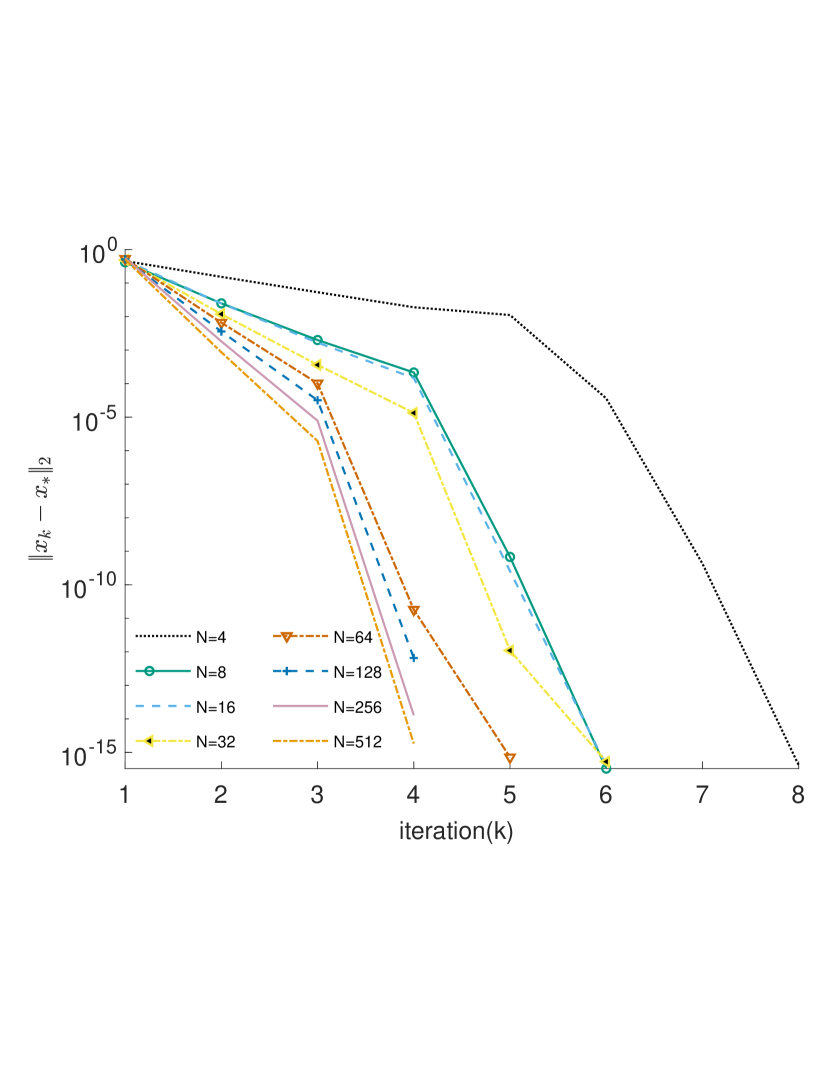
(a) Convergence of $x_{k}$

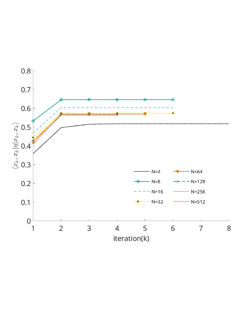
(b) Monotone increasing of $\langle x_{k},x_{k}\rvert\eta\lvert x_{k},x_{k}\rangle$

Figure 1: Convergence behaviour of Alg. 3 for Example 3

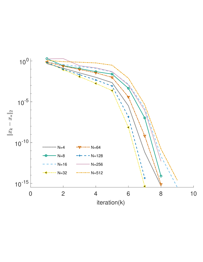
(a) Convergence of $x_{k}$

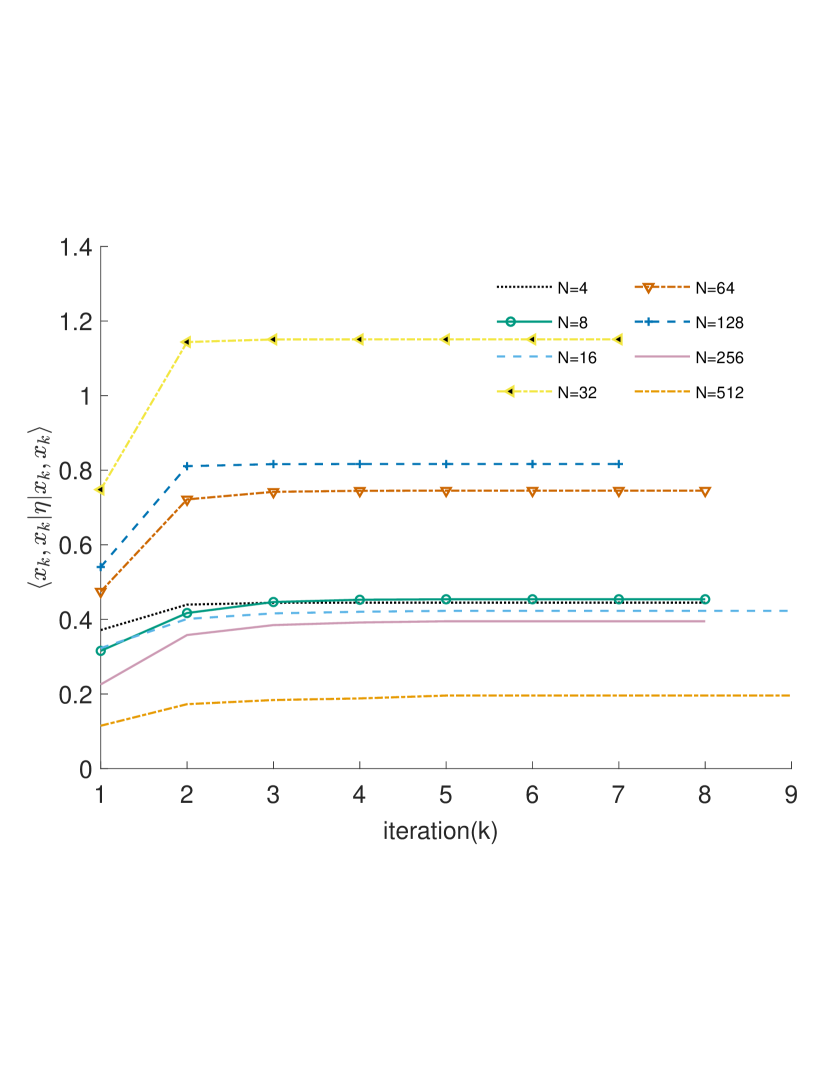
(b) Monotone increasing of $\langle x_{k},x_{k}\rvert\eta\lvert x_{k},x_{k}\rangle$

Figure 2: Convergence behaviour of Alg. 3 for Example 4

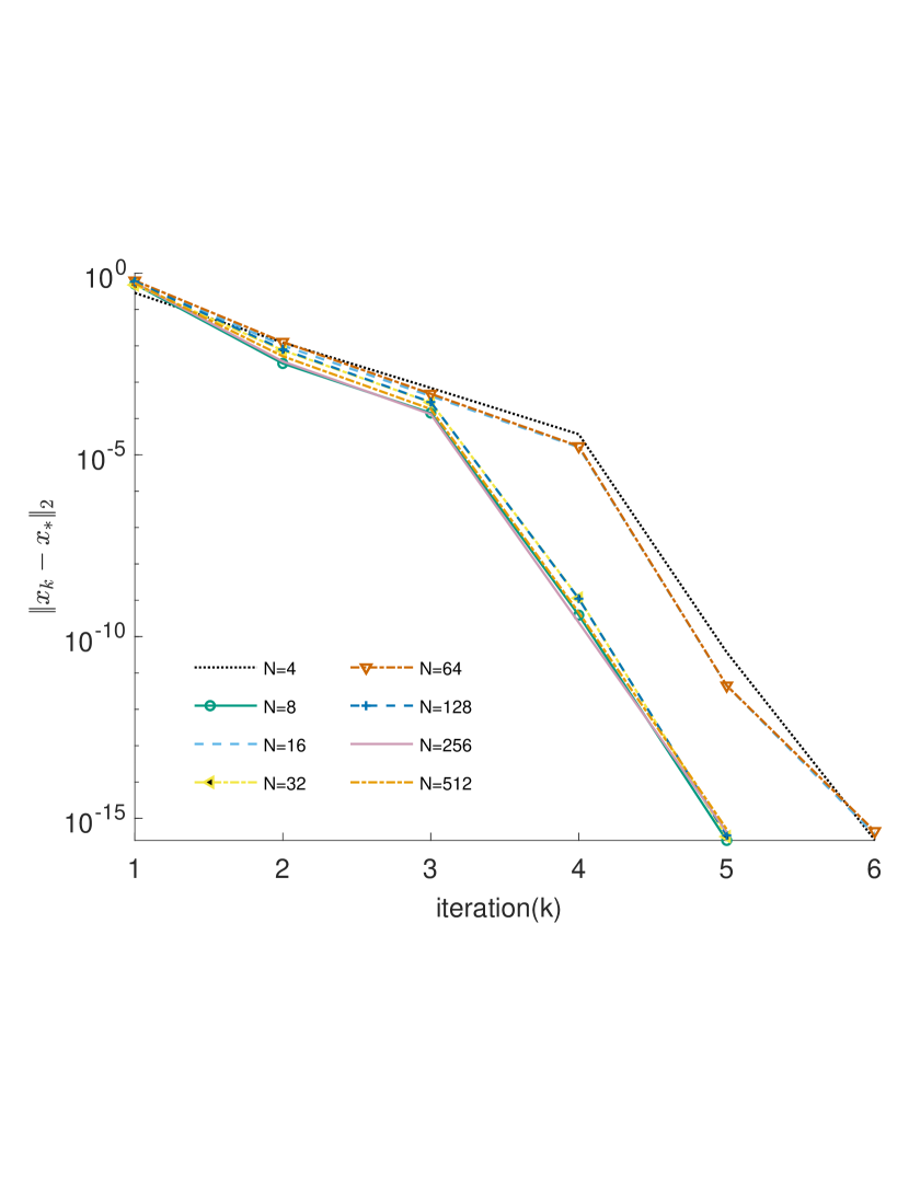
(a) Convergence of $x_{k}$

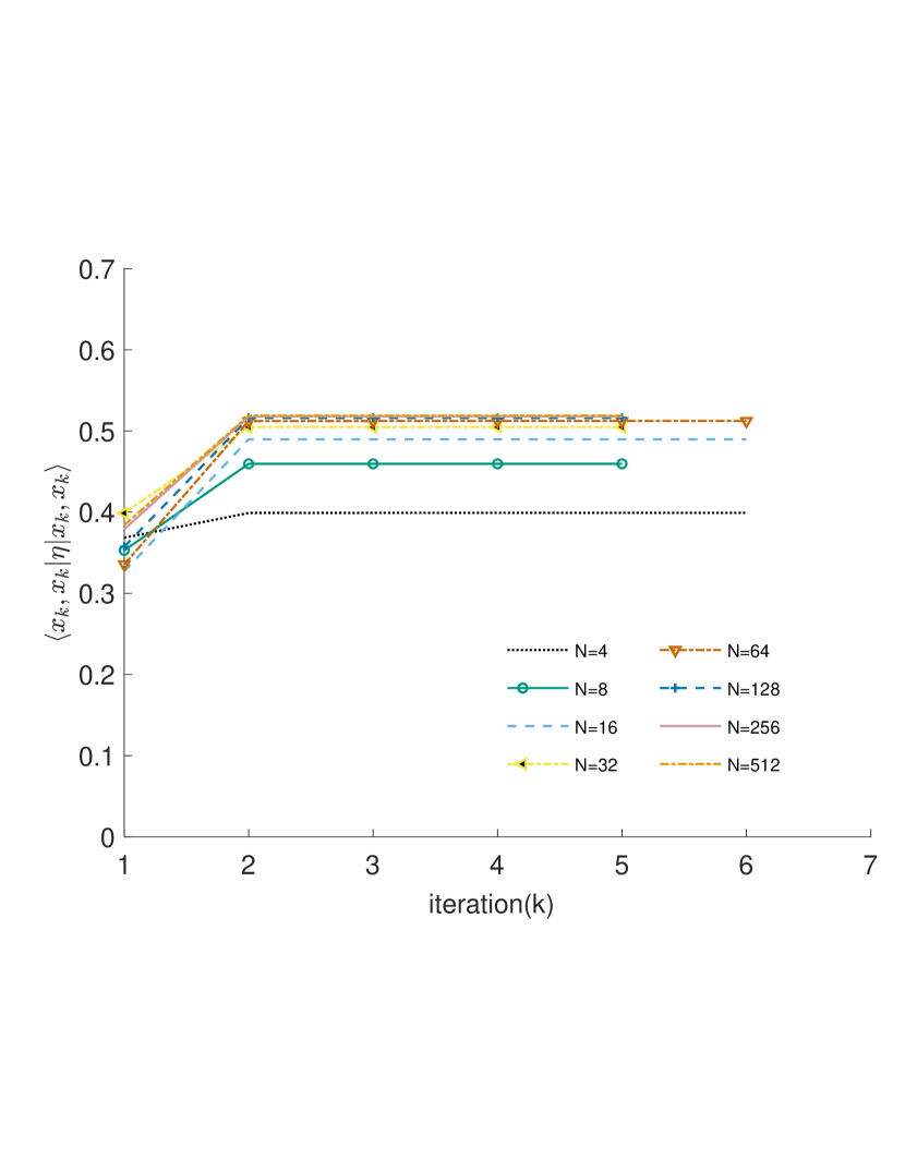
(b) Monotone increasing of $\langle x_{k},x_{k}\rvert\eta\lvert x_{k},x_{k}\rangle$

Figure 3: Convergence behaviour of Alg. 3 for Example 5

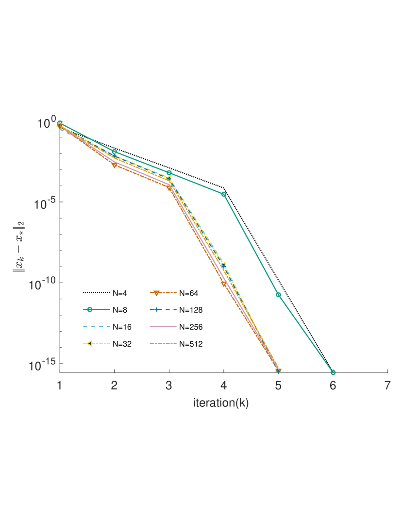
(a) Convergence of $x_{k}$

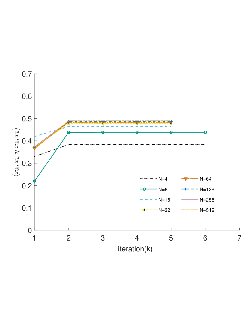
(b) Monotone increasing of $\langle x_{k},x_{k}\rvert\eta\lvert x_{k},x_{k}\rangle$

Figure 4: Convergence behaviour of Alg. 3 for Example 6

From these figures, we can see that the Algorithm 3 converges globally and locally quadratically. And the iteration number of Algorithm 3 will not increase with the dimension of matrix $\eta$. Besides, $\langle x_{k},x_{k}\rvert\eta\lvert x_{k},x_{k}\rangle$ is monotonically increasing, which converges to a local maximum of the optimization problem (83). In practice, in order to save the memory when the matrix size is very large, we don not generate $\eta$. For Example 3 and 4, only $\lambda_{i},x_{i}$ is saved. Then the gradient vector and Hessian matrix can be calculated directly by these gradients. For Example 5 and 6, we have explicit formula to calculate the gradient vector and Hessian matrix. One problem in this algorithm is that we cannot guarantee that the local maximum found is the global maximum. It requires further research to propose a global optimization algorithm.

We also test Algorithm 1 by choosing $\rho$ as $\eta$ as in Example 3,4,5, and 6. Note that, in Example 3, the closest S-separable state of $\rho$ is $\rho$ itself, the distance $\left\lVert\rho-\mathrm{Proj}_{\mathcal{S}}(\rho)\right\rVert_{F}$ is thus $0$. For Example 4,5, abd 6, the distance $\left\lVert\rho-\mathrm{Proj}_{\mathcal{S}}(\rho)\right\rVert_{F}$ is not 0, which implies that these states are not S-separable. We compare the different results for $N=4,8,16,\ldots,512$.

Some parameters for Algorithm 1 are set as follows:

Variables	Value	Meaning
$\epsilon_{1}$	$10^{-12}$	Tolerance in Alg. 1
$\epsilon_{3}$	$10^{-12}$	Tolerance in Alg. 3.
$N_{\max}$	1000	Maximal iteration number in Alg. 1
$\tilde{N}_{\max}$	500	Maximal iteration number in Alg. 3
$x_{0}$	rand(N,1)	Initial vector in Alg. 3
$\rho_{0}$	zeros(N*N)	Initial candidate in Alg. 1

Table 2: Parameters in Algorithm 1

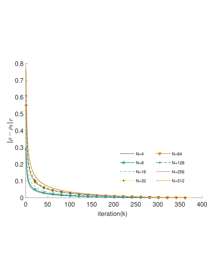
Figure 5: $\left\lVert\rho-\rho_{k}\right\rVert_{F}$ in Example 3

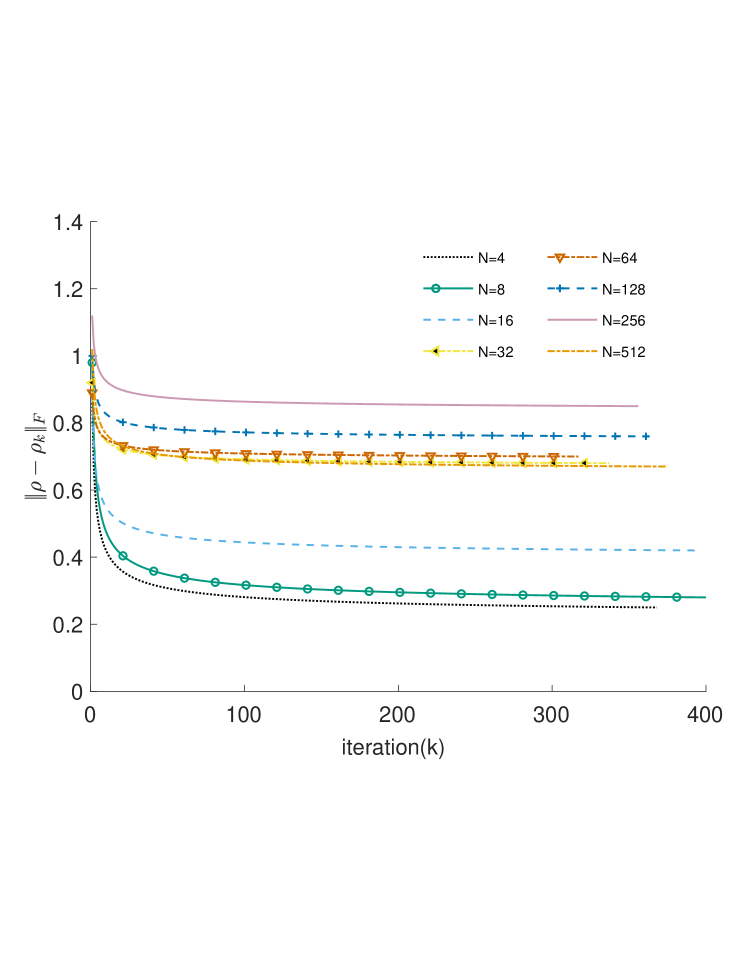
Figure 6: $\left\lVert\rho-\rho_{k}\right\rVert_{F}$ in Example 4

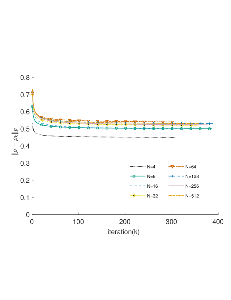
Figure 7: $\left\lVert\rho-\rho_{k}\right\rVert_{F}$ in Example 5

Figure 8: $\left\lVert\rho-\rho_{k}\right\rVert_{F}$ in Example 6

8 Improvement of the Algorithm 1

In fact, we can accelerate the convergence by solving the following quadratic programming

$$\begin{array}[t]{rl}\max\limits_{\lambda_{i}}&\left\lVert\rho-\sum\limits_{i=0}^{k-1}\lambda_{i}\lvert x_{i},x_{i}\rangle\langle x_{i},x_{i}\rvert\right\rVert_{F}\\ \text{ s.t.}&\lambda_{i}\geqslant 0,i=0,1,\ldots,k-1,\end{array}$$ (171)

at $k$-th step to update the coefficient of $\rho_{k}$, which is closer to $\rho$.

Note that the Algorithm 1 may not continue if a small local maximum of $\langle x,x|\rho-\rho_{k}|x,x\rangle$ on the unit sphere is found such that

$$\langle\rho-\rho_{k},\lvert x,x\rangle\langle x,x\rvert-\rho_{k}\rangle<0.$$ (172)

Therefore, global optimization algorithm is need to guarantee the convergence of Algorithm 1. For example, the multi-start strategy can be used to have better results then just using Algorithm 3.

In order to be specific, we consider in this paper mostly the real matrices, however, our algorithm can be easily generalized to real case. It turns out that the states in complex case is the bosonic states, that is the states in the system of indistinguishable particles Eckert_2002 . For a bosonic state $\rho$, it is separable if and only it can be written as

$$\rho=\sum_{i}\lambda_{i}\lvert x_{i},x_{i}\rangle\langle x_{i},x_{i}\rvert$$ (173)

where $\lvert x_{i}\rangle\in\mathbb{C}^{N}$. Algorithm 1 can be generalized to the complex case only if we modify the transposition of real operators to Hermitian conjugation of complex operators. Algorithm 3 can also be generalized to the complex case, that it find the maximum value of

$$\langle x_{i},x_{i}\rvert\sigma\lvert x_{i},x_{i}\rangle,$$ (174)

with $\sigma$ being a matrices in the indistinguishable system. We can utilize the Wirtinger calculus wirtinger1927formalen to compute the gradient vectors and Hessian matrices. The Algorithm 3 thus can be modified accordingly.

It should also be noted that our algorithm can be extended easily to multipartite case, where we need only calculate the gradient vector and Hessian maxtrix and modify the Algorithm 3 and 1 respectively. In order to be concise, we omit describing the implementation details here.

9 Conclusion

In this paper, we consider a subclass of quantum states in the $N\otimes N$ space, namely, the completely symmetric states, which is a similar conception of “supersymmetric tensor” originally in the filed of tensor decomposition. Inspired by the special structure, we conjecture that the completely symmetric state is separable if and only if it is S-separable, which is proved to be true when the rank is less than $4$ or $N+1$. However, it need further research to check whether the validness of this conjecture.

Besides, we propose a numerical algorithm which is able to detect such property with the convergence behavior analyzed. The numerical results show our algorithm is efficient. Furthermore, our algorithm is suitable to check the separability of the Bosonic states. Our algorithm is hopeful to be a aided tool to the study of entanglement in the symmetric system.

In the future work, Conjecture 1 should be investigated in more complicate cases, for example, the states are supported in the higher dimensional space or of higher ranks. It is also of interest to consider this problem in the multipartite system. Another interesting problem is the consider which kind of states can be transformed to the completely symmetric states by the invertible local operator. The Example 1 and 2 are two kind states which satisfy this condition.

Appendix A Proof of Eq.  (104)

In this appendix, we prove Eq. (104). Let us describe this question formally with a lemma.

Lemma 29

Let $x_{*}$ and $x_{\bot}$ are two orthogonal unit vectors in the ^N space and

$$x=\cos(\theta)x_{*}+\sin(\theta)x_{\bot},\theta\in[0,2\pi].$$ (175)

Then we have

$$\left|\sin(\theta)\right|=\sqrt{\left\lVert x-x_{*}\right\rVert^{2}-\frac{\left\lVert x-x_{*}\right\rVert^{4}}{4}}.$$ (176)

Proof

The following graph shows the relations of $x$,$x_{*}$, and $x_{\bot}$ when $\langle x,x_{*}\rangle>0$ (left one) and $\langle x,x_{*}\rangle<0$ (right one):

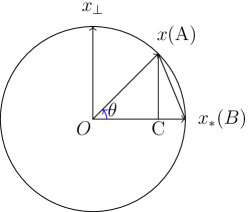
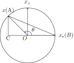
Figure 9: $x=\cos(\theta)x_{*}+\sin(\theta)x_{\bot}$

From the above graphs, we have

$$\left\lVert x-x_{*}\right\rVert=\left|AB\right|.$$ (177)

And

$$\begin{split}\left|OC\right|&=\left|\cos(\theta)\right|,\\ \left|BC\right|&=1-\cos(\theta),\\ \left|AC\right|&=\sin(\theta).\end{split}$$ (178)

Moreover,

$$\begin{split}\left|AB\right|&=\sqrt{\left|AC\right|^{2}+\left|BC\right|^{2}}\\ &=\sqrt{(1-\cos(\theta))^{2}+\sin^{2}(\theta)}\\ &=\sqrt{2-2\cos(\theta)}.\end{split}$$ (179)

Therefore,

$$\cos(\theta)=1-\frac{\left|AB\right|^{2}}{2}.$$ (180)

Forward,

$$\begin{split}\left|\sin(\theta)\right|&=\sqrt{1-\cos^{2}(\theta)}\\ &=\sqrt{1-(1-\frac{\left|AB\right|^{2}}{2})^{2}}\\ &=\sqrt{\left|AB\right|^{2}-\frac{\left|AB\right|^{2}}{4}}\\ &=\sqrt{\left\lVert x-x_{*}\right\rVert^{2}-\frac{\left\lVert x-x_{*}\right\rVert^{4}}{4}}.\end{split}$$ (181)

Appendix B Proof of Eq. (162)

In this appendix, we prove Figure 162, that is to prove

$$\left\lVert x_{\text{\tiny SQP}}-x_{*}\right\rVert\leqslant\left\lVert x_{\text{\tiny NT}}-x_{*}\right\rVert,$$ (182)

where $\left\lVert x_{\text{\tiny SQP}}\right\rVert\leqslant\left\lVert x_{\text{\tiny NT}}\right\rVert$ and $x_{*},x_{\text{\tiny SQP}}$ are unit vectors. The following Figure 10 shows the relationship of $x_{\text{\tiny SQP}}$ and $x_{\text{\tiny NT}}$.

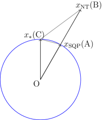
Figure 10: Relation between $x_{\text{\tiny SQP}}$ and $x_{\text{\tiny NT}}$

Note that

$$\angle OAC=\frac{1}{2}(\pi-\angle AOC).$$ (183)

Hence,

$$\begin{split}\angle BAC&=\pi-\angle OAC\\ &=\pi-\frac{1}{2}(\pi-\angle AOC)\\ &=\frac{\pi}{2}+\frac{1}{2}\angle AOC\\ &>\frac{\pi}{2}.\end{split}$$ (184)

Moreover,

$$\sin(\angle ABC)\leqslant\sin(\pi-\angle BAC)=\sin(\angle BAC).$$ (185)

Forward,

$$\frac{\left\lVert x_{\text{\tiny SQP}}-x_{*}\right\rVert}{\left\lVert x_{NT}-x_{*}\right\rVert}=\frac{\sin(\angle ABC)}{\sin(\angle BAC)}.$$ (186)

By Eq. 185, we have

$$\frac{\left\lVert x_{\text{\tiny SQP}}-x_{*}\right\rVert}{\left\lVert x_{NT}-x_{*}\right\rVert}\leqslant 1,$$ (187)

which completes our proof.

References

- (1) A. Einstein, B. Podolsky, and N. Rosen. Can quantum-mechanical description of physical reality be considered complete? Phys. Rev., 47(10):777–780, May 1935.
- (2) Erwin Schrödinger. Die gegenwärtige situation in der quantenmechanik. Naturwissenschaften, 23(49):823–828, 1935.
- (3) Michael A. Nielsen and Isaac L. Chuang. Quantum information theory, 2002.
- (4) Leonid Gurvits. Classical deterministic complexity of edmonds’ problem and quantum entanglement. In Proceedings of the thirty-fifth ACM symposium on Theory of computing - STOC ’03, pages 10–19. ACM, ACM Press, 2003.
- (5) Sevag Gharibian. Strong NP-hardness of the quantum separability problem. arXiv preprint arXiv:0810.4507, 2008.
- (6) Asher Peres. Separability criterion for density matrices. Phys. Rev. Lett., 77(8):1413–1415, August 1996.
- (7) Michał Horodecki, Paweł Horodecki, and Ryszard Horodecki. Separability of mixed states: Necessary and sufficient conditions. Phys. Lett. A, 223(1-2):1–8, November 1996.
- (8) S.L. Woronowicz. Positive maps of low dimensional matrix algebras. Rep. Math. Phys., 10(2):165–183, October 1976.
- (9) Michał Horodecki, Paweł Horodecki, and Ryszard Horodecki. Separability of mixed quantum states: Linear contractions and permutation criteria. Open Syst. Inf. Dyn., 13(01):103–111, March 2006.
- (10) Dariusz Chruściński, Jacek Jurkowski, and Andrzej Kossakowski. Quantum states with strong positive partial transpose. Phys. Rev. A, 77(2):022113, 2008.
- (11) Kil-Chan Ha. Entangled states with strong positive partial transpose. Phys. Rev. A, 81(6):064101, 2010.
- (12) Lilong Qian. Separability of multipartite quantum states with strong positive partial transpose. Phys. Rev. A, 98:012307, Jul 2018.
- (13) B. Kraus, J. I. Cirac, S. Karnas, and M. Lewenstein. Separability in2Ncomposite quantum systems. Phys. Rev. A, 61(6):062302, May 2000.
- (14) Paweł Horodecki, Maciej Lewenstein, Guifré Vidal, and Ignacio Cirac. Operational criterion and constructive checks for the separability of low-rank density matrices. Phys. Rev. A, 62(3):032310, August 2000.
- (15) Shao-Ming Fei, Xiu-Hong Gao, Xiao-Hong Wang, Zhi-Xi Wang, and Ke Wu. Separability and entanglement in composite quantum systems. Phys. Rev. A, 68(2):022315, 2003.
- (16) Ming Li, Jing Wang, Shao-Ming Fei, and Xianqing Li-Jost. Quantum separability criteria for arbitrary-dimensional multipartite states. Phys. Rev. A, 89:022325, Feb 2014.
- (17) Andrew C. Doherty, Pablo A. Parrilo, and Federico M. Spedalieri. Complete family of separability criteria. Phys. Rev. A, 69(2):022308, February 2004.
- (18) L. M. Ioannou, B. C. Travaglione, D. C. Cheung, and A. K. Ekert. Improved algorithm for quantum separability and entanglement detection. Phys. Rev. A, 70:060303, Dec 2004.
- (19) Geir Dahl, Jon Magne Leinaas, Jan Myrheim, and Eirik Ovrum. A tensor product matrix approximation problem in quantum physics. Linear Algebra and its Applications, 420(2-3):711–725, January 2007.
- (20) Dimitri P Bertsekas. Nonlinear programming. Athena scientific Belmont, 1999.
- (21) Eleftherios Kofidis and Phillip A Regalia. On the best rank-1 approximation of higher-order supersymmetric tensors. SIAM Journal on Matrix Analysis and Applications, 23(3):863–884, 2002.
- (22) Liqun Qi. Eigenvalues of a real supersymmetric tensor. Journal of Symbolic Computation, 40(6):1302–1324, December 2005.
- (23) Tamara G Kolda and Brett W Bader. Tensor decompositions and applications. SIAM rev., 51(3):455–500, 2009.
- (24) Lin Chen and Dragomir Ž Đoković. Dimensions, lengths, and separability in finite-dimensional quantum systems. J. Math. Phys., 54(2):022201, February 2013.
- (25) Lin Chen and Dragomir Ž Đoković. Distillability and PPT entanglement of low-rank quantum states. J. Phys. A: Math. Theor., 44(28):285303, June 2011.
- (26) Lin Chen and Dragomir Ž Đoković. Properties and construction of extreme bipartite states having positive partial transpose. Commun. Math. Phys., 323(1):241–284, July 2013.
- (27) Angelia Nedić Bertsekas, Dimitri P. and Asuman E. Ozdaglar. Convex Analysis and Optimization, volume 1. Athena scientific Belmont, 2005.
- (28) Mokhtar S. Bazaraa, Hanif D. Sherali, and C. M. Shetty. Nonlinear Programming. John Wiley & Sons, Inc., October 2005.
- (29) Vasilis Pagonis, George Kitis, and Claudio Furetta. Numerical and Practical Exercises in Thermoluminescence. Springer New York, New York, NY, 2006.
- (30) Liqun Qi, Fei Wang, and Yiju Wang. Z-eigenvalue methods for a global polynomial optimization problem. Math. Program., 118(2):301–316, September 2007.
- (31) K. Eckert, J. Schliemann, D. Bruß, and M. Lewenstein. Quantum correlations in systems of indistinguishable particles. Ann. Phys., 299(1):88–127, jul 2002.
- (32) Wilhelm Wirtinger. Zur formalen theorie der funktionen von mehr komplexen veränderlichen. Math. Ann., 97(1):357–375, 1927.
- (33) Yu Guan, Moody T Chu, and Delin Chu. SVD-based algorithms for the best rank-1 approximation of a symmetric tensor. SIAM J. Matrix Anal. Appl., 39(3):1095–1115, 2018.
- (34) Yu Guan, Moody T Chu, and Delin Chu. Convergence analysis of an SVD-based algorithm for the best rank-1 tensor approximation. Linear Algebra Appl., 2018.
- (35) C Hao, C Cui, and Y Dai. A feasible trust-region method for calculating extreme z-eigenvalues of symmetric tensors. Pacific Journal of Optimization, 11(2):291–307, 2015.
- (36) Guoyin Li, Liqun Qi, and Gaohang Yu. The z-eigenvalues of a symmetric tensor and its application to spectral hypergraph theory. Numerical Linear Algebra with Applications, 20(6):1001–1029, 2013.