Accelerating Stochastic Gradient Descent Using Antithetic Sampling

Abstract

(Mini-batch) Stochastic Gradient Descent is a popular optimization method which has been applied to many machine learning applications. But a rather high variance introduced by the stochastic gradient in each step may slow down the convergence. In this paper, we propose the antithetic sampling strategy to reduce the variance by taking advantage of the internal structure in dataset. Under this new strategy, stochastic gradients in a mini-batch are no longer independent but negatively correlated as much as possible, while the mini-batch stochastic gradient is still an unbiased estimator of full gradient. For the binary classification problems, we just need to calculate the antithetic samples in advance, and reuse the result in each iteration, which is practical. Experiments are provided to confirm the effectiveness of the proposed method.

1 Introduction

In this big data era, many machine learning applications involve a large number of samples. To solve these problems effectively, Stochastic Gradient Descent (SGD) is a desired method and has been extensively studied in the machine learning community Bottou et al. (2016); Allen-Zhu (2017); Duchi et al. (2010); Johnson and Zhang (2013); Zhao and Zhang (2015). In each iteration, a typical SGD will draw one sample from training data to calculate the stochastic gradient. The stochastic gradient is an unbiased estimator of full gradient. A nature modification is to employ the mini-batch training, which draws several samples to calculate the mini-batch stochastic gradient. And the mini-batch stochastic gradient is also unbiased. In the traditional mini-batch SGD setting, each sample is drew independently to compose the mini-batch, which will lead to a rather high variance. The variance may weaken the performance of SGD. In this paper, we introduce the antithetic sampling strategy to SGD to reduce the variance, while keeping the unbiased property of stochastic gradient.

In order to induce a smaller variance, the requirement of independence between every two samples inside a mini-batch is removed in our method. Exactly, if the two stochastic gradients derived from two samples are negatively correlated, then they would generate a mini-batch stochastic gradient with smaller variance. In other words, a smaller variance of this mini-batch stochastic gradient is foreseeable when the inner product of these two stochastic gradients being smaller in the expectation. We regard such two samples are antithetic to each other. The mutually antithetic samples compose the mini-batch in our method. Unlike the stratified sampling in SGD which needs a relatively big mini-batch Zhao and Zhang (2014), the size of mini-batch required in the antithetic sampling is quiet flexible: it just need to be bigger than $1$.

To get the antithetic samples, one need to calculate the inner products between every two stochastic gradients in each step, which is inefficient. A more practical approach is to relax the problem: we turn to reduce the bound of the inner product to expect a smaller inner product. For the binary classification problem, the bound can be easily got, and it is independent of optimization variables. As a result, we just need to do calculations beforehand to get the antithetic table which records the information of antithetic samples, and reuse this table in each iteration. Since some multi-class classification problems can be split into several binary classification problems to solve Aly (2005), our method can be expanded to these multi-class classification problems. Besides, our method is complementary to other variance reduction methods Johnson and Zhang (2013); Zhao and Zhang (2014, 2015). In fact, different variance reduction methods can be combined to use.

The rest of this paper is organized as follows. Section 2 reviews the related work. In section 3, we will analyse the impacts of variance to convergence performance, and introduce the antithetic sampling strategy to SGD. In section 4, we relax the problem of calculating antithetic samples, and propose practical methods for the common binary classification problems. The empirical evaluations are presented in section 5. Section 6 concludes the paper.

2 Related Work

Stochastic Gradient Descent (SGD) was studied long ago Robbins and Monro (1951). And in recent years, SGD has been widely used to minimize the empirical risk in machine learning community Shalev-Shwartz et al. (2007); Shamir and Zhang (2013); Bottou et al. (2016). Although the use of stochastic gradient makes SGD has low per iteration cost, a rather high variance introduced by the stochastic gradient will slow down the convergence.

To effectively reduce the variance of stochastic gradient in SGD, some variance reduction methods in statistics, such as importance sampling, control variates and stratified sampling Ross (2013); Owen (2013), were introduced to stochastic optimization problems. We divide the related work for variance reduction in SGD into two categories:

1. From the aspect of optimization variable.

2. Form the aspect of dataset.

SVRG Johnson and Zhang (2013), SAGA Defazio et al. (2014) and SDCA Shalev-Shwartz and Zhang (2013) can be regarded as the variance reduction methods from the aspect of optimization variable. All of them can reduce the variance to 0 asymptotically. SVRG and SAGA adopt the control variate method to reduce variance. The control variates in both algorithms are the stochastic gradients with respect to the optimization variables of a previous step. SDCA can be regarded as adopting antithetic sampling to reduce variance as explained in Johnson and Zhang (2013). The convergence properties of these methods are different from that of SGD. So, generally, we regard them as different methods.

On the other hand, utilizing the internal structure of dataset to proceed variance reduction was considered in Wang et al. (2013); Zhao and Zhang (2014, 2015). In Wang et al. (2013), the control variates were constructed via low-order approximations to the stochastic gradient. Zhao and Zhang (2014) utilized the clustering information of dataset to divide the whole dataset into clusters and performed the stratified sampling. While Zhao and Zhang (2015) studied the importance sampling in SGD, where an nonuniform sampling distribution is constructed according to the internal structure of dataset. Stich et al. (2017); Zhu (2016) developed the importance sampling methods further. Although these methods may not reduce the variance to 0, they can be regarded as complementary to other variance reduction methods.

The above variance reduction methods can be used in combination. Xiao and Zhang (2014); Shen et al. (2016) applied importance sampling to SVRG. Csiba et al. (2015) proposed a variant of SDCA, which also combined the importance sampling methods. Allen-Zhu et al. (2016) improved SVRG by exploiting clustering structure inside datasets.

This paper introduces a new method that utilizes the antithetic sampling to reduce the variance in SGD. This method is complementary to the existing variance reduction methods.

3 SGD with Antithetic Sampling

3.1 Problem Setting

In this paper, we focus on the binary classification task with a set of samples $\{(x_{1},y_{1}),(x_{2},y_{2}),\dots,(x_{n},y_{n})\}$, where each $x_{i}\in\mathbb{R}^{d}$ is a $d$-dimensional instance and $y_{i}$ is the corresponding class label assigned to $x_{i}$. For a sample $(x_{i},y_{i})$, the loss function $f_{i}(w)$ from $\mathbb{R}^{d}$ to $\mathbb{R}$ is introduced. To learn the classifier, we need to find an approximate solution of the following optimization problem

$$\min\limits_{w\in\mathbb{R}^{d}}f(w):=\frac{1}{n}\sum\limits_{i=1}^{n}f_{i}(w)$$ (1)

Stochastic Gradient Descent (SGD) is a popular method to solve the above optimization problem, it is an iterative algorithm. At each iteration $t=1,2,\dots$, an index $i_{t}$ will be uniformly randomly sampled from $\{1,2,\dots,n\}$, then $w$ will be updated as

$$w_{t+1}=w_{t}-\eta_{t}\nabla\!f_{i_{t}}(w_{t}),$$ (2)

where $\eta_{t}$ is a positive stepsize.

The batch approach is a nature modification. For a mini-batch of indices $\mathcal{B}_{t}$ with size $b$, the update of $w$ is

$$w_{t+1}=w_{t}-\frac{\eta_{t}}{b}\sum\limits_{s\in\mathcal{B}_{t}}\nabla\!f_{s}(w_{t}),$$ (3)

where $\mathcal{B}_{t}=\{i_{t}^{j}\in\{1,2,\dots,n\}|j=1,2,\dots,b\}$ is i.i.d. uniformly sampled with replacement from the set of indices. This sampling process is the distinction to the way in our antithetic sampling.

In the rest of this paper, we’ll use SGD to refer to both SGD and mini-batch SGD cases. The stochastic gradients are unified as $g_{t}$. Then, we can unify (2) and (3) as:

$$w_{t+1}=w_{t}-\eta_{t}g_{t},$$ (4)

The expectation of a random variable $X$ is denoted by $\mathbb{E}[X]$. While we use $\mathbb{E}_{t}[\cdot]$ to denote an expected value taken with respect to $\{i_{t}^{j}|j=1,2,\dots,b\}$, the random variable appeared in $t$-th iteration. Note that $g_{t}$ is an unbiased estimator of the full gradient,

$$\mathbb{E}_{t}[g_{t}]=\nabla f(w)=\frac{1}{n}\sum\limits_{i=1}^{n}f_{i}(w).$$ (5)

In this paper, we’ll keep this unbiased property.

3.2 Impacts of Variance

In this subsection, we analyse the impacts of variance in SGD from the general perspective. The analysis covers a variety of situations based on different assumptions, such as convex, strongly convex and smoothness.

For the random vector $g_{t}$, we denote the variance

$$\text{Var}(g_{t})=\mathbb{E}_{t}\!\left\|g_{t}-\mathbb{E}_{t}g_{t}\right\|^{2}=\mathbb{E}_{t}\!\left\|g_{t}\right\|^{2}-\left\|\mathbb{E}_{t}g_{t}\right\|^{2}.$$ (6)

Since $\mathbb{E}_{t}g_{t}=\nabla f(w_{t})$, which is identical under different sampling process, we’ll use the second moment $\mathbb{E}_{t}\!\left\|g_{t}\right\|^{2}$ to refer to the variance. For the smooth optimization problem, the Lipschitz continuous gradient assumption is usually used to describe the smoothness of the function.

Formally, if $f$ has the Lipschitz continuous gradient with parameter $L$, then for any $x,y\in\mathbb{R}^{d}$, we have

$$f(x)\leq f(y)+\left<\nabla\!f(y),x-y\right>+\frac{L}{2}\left\|x-y\right\|^{2}.$$ (7)

Lipschitz continuous gradient assumption is widely used. It establishes convergence guarantee for stochastic gradient on an assumption of smoothness of the objective function.

By the inequality (7), the iterations of SGD satisfy

$$f(w_{t+1})\!-\!f(w_{t}) \leq \left<\nabla\!f(w_{t}),w_{t+1}\!-\!w_{t}\right>\!+\!\frac{L}{2}\left\|w_{t+1}\!-\!w_{t}\right\|^{2}$$

$$= -\eta_{t}\left<\nabla\!f(w_{t}),g_{t}\right>+\frac{L}{2}\eta_{t}^{2}\left\|g_{t}\right\|^{2}.$$

Taking expectations in these inequalities, we can get

$$\mathbb{E}_{t}f(w_{t+1})-f(w_{t})\leq-\eta_{t}\left\|f(w_{t})\right\|^{2}+\frac{L}{2}\eta_{t}^{2}\mathbb{E}_{t}\!\left\|g_{t}\right\|^{2}.$$ (8)

So with bounded variance, under proper stepsize, the decrease of $f$ can be guaranteed in the statistical sense. The smaller the variance is, the larger the stepsize that can be adopted, which will result in a faster decrease of $f$.

Some machine learning applications involve non-smooth loss functions without Lipschitz smooth assumption, for example, the support vector machine with the standard non-smooth hinge loss Shalev-Shwartz et al. (2007). SGD can also work by denoting $g_{t}$ as a subgradient Shamir and Zhang (2013). According to the iterative process of SGD, we have

$$\mathbb{E}_{t}[\left\|w_{t+1}-w^{*}\right\|^{2}]$$ (9)

$$= \left\|w_{t}-w^{*}\right\|^{2}-2\eta_{t}\mathbb{E}_{t}\!\left<g_{t},w_{t}-w^{*}\right>+\eta_{t}^{2}\mathbb{E}_{t}\!\left\|g_{t}\right\|^{2}$$

Similar to previous analysis, a smaller variance will allow a faster rate of $w$ toward the optimal point.

$f(w)$ or $\|w-w^{*}\|^{2}$ may not decrease effectively if $\mathbb{E}_{t}\|g_{t}\|^{2}$ is rather big. So in most convergence rate analyses of SGD Bottou et al. (2016); Shamir and Zhang (2013), a common assumption is

$$\mathbb{E}\left\|g_{t}\right\|^{2}\leq G^{2},\;\;\;t=1,2,\dots$$ (10)

This assumption corresponds to a bounded variance. It is made to ensure the effects of variance can be offset by the decreasing stepsize.

For the convergence rate, what we are concern about is the upper bound of $\mathbb{E}f(w_{t})-f(w^{*})$ or $\mathbb{E}[\left\|w_{t+1}-w^{*}\right\|^{2}]$. Commonly, (8) and (9) would appear in the analysis of convergence rate. This makes the upper bound to be related to the variance of stochastic gradient. Generally, the upper bound is proportional to $G^{2}$. A smaller variance generated in each steps will decrease the upper bound of $\mathbb{E}\!\left\|g_{t}\right\|^{2}$. Then $G^{2}$ will be a smaller value, which will lead to a faster convergence.

Remark. For the optimization problem with a non-smooth regularization term $r$:

$$\min\limits_{w\in\mathbb{R}^{d}}P(w):=\frac{1}{n}\sum\limits_{i=1}^{n}f_{i}(w)+r(w),$$ (11)

SGD with proximal operation (Prox-SGD) can be used to solve it. In this case, the variance of stochastic gradient has a similar influence on convergence rate Duchi et al. (2010). So, the analyses of variance reduction for (1) are still applicable.

3.3 Antithetic Sampling

In this subsection, we’ll introduce the antithetic sampling strategy to reduce the variance.

Without loss of generality, we consider mini-batch SGD with batch size 2. In this case,

$$g_{t}=\frac{1}{2}\left(\nabla\!f_{i}(w_{t})+\nabla\!f_{j}(w_{t})\right),\;i,j\in\{1,2,\dots,n\}.$$ (12)

In the traditional setting, $i$ and $j$ are i.i.d., then

$$\text{Var}(g_{t}) = \frac{1}{4}\left(\text{Var}(\nabla\!f_{i}(w_{t}))+\text{Var}(\nabla\!f_{j}(w_{t}))\right)$$ (13)

$$= \frac{1}{2}\text{Var}(\nabla\!f_{i}(w_{t}))$$

If we adopt a new sampling strategy in which $i$ and $j$ may not independent, but still have identically distribution. Then we have

$$\text{Var}(g_{t})=\frac{1}{2}\left\{\text{Var}(\nabla\!f_{i}(w_{t}))+\text{Cov}(\nabla\!f_{i}(w_{t}),\nabla\!f_{j}(w_{t}))\right\},$$ (14)

where

$$\text{Cov}(\nabla\!f_{i}(w_{t}),\nabla\!f_{j}(w_{t}))$$

$$= \mathbb{E}_{t}\!\left\{\nabla f_{i}(w_{t})^{T}\nabla f_{j}(w_{t})\right\}\!-\!\mathbb{E}_{t}[\nabla f_{i}(w_{t})]^{T}\mathbb{E}_{t}[\nabla f_{j}(w_{t})]$$

If $\text{Cov}(\nabla\!f_{i}(w_{t}),\nabla\!f_{j}(w_{t}))\!<\!0$, which means $\nabla f_{j}(w_{t})$ may be the one that somehow indicates the opposite direction of $\nabla f_{i}(w_{t})$, then we can derive the stochastic gradient $g_{t}$ with smaller variance. And the closer $\nabla f_{j}(w_{t})$ and $2\mathbb{E}_{t}[g_{t}]\!-\!\nabla f_{i}(w_{t})$, the better we can expect to reduce more variance. Such stochastic gradients $\nabla f_{i}(w_{t})$ and $\nabla f_{j}(w_{t})$ can be regarded as negative correlated. Since $i$ and $j$ have identically distribution, $g_{t}$ is still an unbiased estimator of full gradient. For the negative correlated $\nabla f_{i}(w_{t})$ and $\nabla f_{j}(w_{t})$, we regard corresponding samples $i$ and $j$ to be antithetic to each other.

In each iteration, it is supposed that we have gotten the pairing information between samples, under which one sample is antithetic to its partner. Then we draw a pair of samples to calculate the mini-batch stochastic gradient. The variance of $g_{t}$ obtained under this process is smaller than that got under tradition i.i.d. uniformly sampling. As we have explained, a smaller variance corresponds to a smaller $\mathbb{E}_{t}\!\left\|g_{t}\right\|^{2}$, which will directly result in a better convergence performance. Figure 1 illustrates the effect of antithetic sampling.

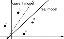
Figure 1: An illustration to explain the effect of antithetic sampling. A, B, C, D are four samples presented, solid line represents the real model we want to get, dotted line represents the model we already got in previous iterations. In the next iteration, suppose we use sample A to train, then the dotted line will tend to A. It is not the direction to the real model as this direction is not obtained through all training samples. If both A and B are selected, then B can rectify the influence of A in some extent, which will make the direction more accurate, then the current model will better approximate the real model. For C, the correction may not as effective as B. However, D will exacerbate the negative impact. So, we can regard B as the antithetic sampling of A in the current iteration.

Algorithm 1 Stochastic Gradient Descent with Antithetic Sampling

1:  for $t=1,2,\ldots,$ do

2:     Get Antithetic Table $S$.

3:     Uniformly sample $i_{t}$ from $\{1,\dots,n\}$;

4:     Get the antithetic sample $j_{t}=S_{i_{t}}$;

5:     Update $w_{t+1}=w_{t}-\frac{\eta_{t}}{2}\left(\nabla\!f_{i_{t}}(w_{t})+\nabla\!f_{j_{t}}(w_{t})\right)$;

6:  end for

Utilizing above ideas, we propose SGD with antithetic sampling (SGD-as), which is shown as Algorithm 1. To implement the antithetic sampling, in each step, for each sample $i\in\{1,\dots,n\}$, we need to get its antithetic sample $j$. All the antithetic information is stored in the table $S$. By denoting $S_{i}=j$, $S$ records the antithesis of all samples. It is a permutation of $\{1,\dots,n\}$ since the unbiased property of mini-batch stochastic gradient. The SGD-as iteration requires the calculation of $S$ at each step, which is clearly inefficient. But for the binary classification, we’ll show that $S$ can be calculated beforehand and reused in each iteration. Although Algorithm 1 considers the case where the batch size is 2, this algorithm can be generalized to the cases with bigger batch size by simply selecting more pairs of antithetic samples.

4 Calculate Antithetic Samples

To conduct the antithetic sampling, we need to calculate the antithetic table. In this section, we’ll show this calculation can be efficient in the binary classification problems. We begin with relaxing the calculations of antithetic samples. After that, some common and exact binary classification applications will be discussed in detail.

4.1 Analysis

For the stochastic gradient with batch size 2 in SGD, we have

$$\mathbb{E}_{t}\!\left\|g_{t}\right\|^{2}=\frac{1}{4}\mathbb{E}_{t}\!\left\|\nabla f_{i}(w_{t})+\nabla f_{j}(w_{t})\right\|^{2}$$

$$= \frac{1}{4}\mathbb{E}_{t}\!\left\{\left\|\nabla f_{i}(w_{t})\right\|^{2}\!+\!\left\|\nabla f_{j}(w_{t})\right\|^{2}\!+\!2\nabla f_{i}(w_{t})^{T}\nabla f_{j}(w_{t})\right\}\!.$$

As only $\mathbb{E}_{t}\!\left[\nabla f_{i}(w_{t})^{T}\nabla f_{j}(w_{t})\right]$ will be affected by the selection of stochastic samples, we just need to consider it. To minimize $\mathbb{E}_{t}\!\left[\nabla f_{i}(w_{t})^{T}\nabla f_{j}(w_{t})\right]$, we need to calculate the antithetic samples of all samples, which can be represented as the following optimization problem:

$$\!\min\limits_{j_{1},j_{2},\dots,j_{n}}\frac{1}{n}\sum\limits_{i=1}^{n}\nabla f_{i}(w_{t})^{T}\nabla f_{j_{i}}(w_{t}),$$ (16)

where $j_{i}$ is the antithetic sample of $i$. Solving this problem requires the calculations of $n$ derivatives in each iteration, which is clearly inefficient. Beyond, this problem itself is difficult to solve. So we seek to reduce $\mathbb{E}_{t}\!\left\|g_{t}\right\|^{2}$ as much as possible rather than minimizing it.

In the traditional SGD setting, $i$ and $j$ are sampled independently, then:

$$\mathbb{E}_{t}\!\left[\nabla f_{i}(w_{t})^{T}\nabla f_{j}(w_{t})\right]=\left[\mathbb{E}_{t}\!\nabla f_{i}(w_{t})\right]^{2}\geq 0,$$ (17)

So for each pair of $i$ and $j$, if we can guarantee

$$\nabla f_{i}(w_{t})^{T}\nabla f_{j}(w_{t})<0,$$ (18)

then we have $\mathbb{E}_{t}\!\left[\nabla f_{i}(w_{t})^{T}\nabla f_{j}(w_{t})\right]\!<\!0$, which will inevitably lead to a smaller $\mathbb{E}_{t}\!\left\|g_{t}\right\|^{2}$ than the traditional setting.

In addition to this ideal case, we can consider relaxing the problem: for an exactly $i$, we aim to sample the $j$ to get a smaller $\nabla f_{i}(w_{t})^{T}\nabla f_{j}(w_{t})$.

For $\nabla f_{i}(w_{t})^{T}\nabla f_{j}(w_{t})>0$, if we can get the upper bound in advance:

$$\nabla f_{i}(w_{t})^{T}\nabla f_{j}(w_{t})<B_{i}B_{j},$$ (19)

then we may get a smaller $\nabla f_{i}(w_{t})^{T}\nabla f_{j}(w_{t})$ by reducing the upper bound. This technique is also used in Zhao and Zhang (2015).

Similarly, for $\nabla f_{i}(w_{t})^{T}\nabla f_{j}(w_{t})<0$, if we can get the lower bound in advance:

$$\nabla f_{i}(w_{t})^{T}\nabla f_{j}(w_{t})>L_{i}L_{j},$$ (20)

then the value of $\nabla f_{i}(w_{t})^{T}\nabla f_{j}(w_{t})$ may be reduced with a smaller lower bound.

In the next subsection, we’ll show that for common binary classification problems, $B_{i},L_{i},\,i\in\{1,2,\dots,n\}$ can be easily obtained and independent of $t$.

Remark. Consider the optimization problem:

$$\min\limits_{w\in\mathbb{R}^{d}}f(w):=\frac{1}{n}\sum\limits_{i=1}^{n}f_{i}(w)=\frac{1}{n}\sum\limits_{i=1}^{n}g_{i}(w)+h(w),$$ (21)

where $h(w)$ is the smooth regularization, e.g. $\frac{\lambda}{2}\left\|w\right\|^{2}$. Intuitively, since $h(w)$ does not involve $i$, it has no impacts on the variance. So we can follow above analysis without considering $h(w)$. Formally,

$$\mathbb{E}_{t}\!\left[\nabla f_{i}(w_{t})^{T}\nabla f_{j}(w_{t})\right]=\mathbb{E}_{t}\!\left[\nabla g_{i}(w_{t})^{T}\nabla g_{j}(w_{t})\right]$$

$$+2\left(\mathbb{E}_{t}\!\nabla g_{i}(w)\right)^{T}\nabla h(w)+\left\|\nabla h(w)\right\|^{2}$$

Only the first term will be affected by the selection of stochastic samples. So we can adopt the above analysis with simply replacing $\nabla f_{i}(w_{t})$ with $\nabla g_{i}(w_{t})$.

4.2 Binary Classification

In this subsection, we consider two common binary classification applications: logistic regression and support vector machine, one contains smooth loss functions while another contains non-smooth loss functions. We’ll show how they correspond to the above analysis.

For the logistic regression problem with $y_{i}\!\in\!\left\{-1,1\right\},\;i=1,\dots,n$, we need to minimize

$$f(w)=\frac{1}{n}\sum\limits_{i=1}^{n}\log\left(1+\exp(-y_{i}\cdot w^{{}^{\prime}}x_{i})\right).$$ (22)

Then the stochastic gradient of sample $i$ can be written as

$$\nabla f_{i}(w)=-\frac{\exp(-y_{i}\cdot w^{{}^{\prime}}x_{i})}{1+\exp(-y_{i}\cdot w^{{}^{\prime}}x_{i})}\cdot y_{i}x_{i}^{{}^{\prime}}.$$ (23)

Since

$$0<\frac{\exp(-y_{i}\cdot w^{{}^{\prime}}x_{i})}{1+\exp(-y_{i}\cdot w^{{}^{\prime}}x_{i})}<1,$$ (24)

For the two samples $i$ and $j$, if

$$y_{i}y_{j}x_{i}^{{}^{\prime}}x_{j}\!<\!0,$$ (25)

then we can get $\nabla f_{i}(w_{t})^{T}\nabla f_{j}(w_{t})\!<\!0$, which is always hold no matter in which step. Further, if for all $i\in\{1,\dots,n\}$, there exists corresponding $j$ to establish (25), then we can get the mini-batch stochastic gradient with a smaller variance according to the previous analysis,

For the more general case, we have

$$0<\nabla f_{i}(w_{t})^{T}\nabla f_{j}(w_{t})<y_{i}y_{j}x_{i}^{{}^{\prime}}x_{j}$$ (26)

or

$$y_{i}y_{j}x_{i}^{{}^{\prime}}x_{j}<\nabla f_{i}(w_{t})^{T}\nabla f_{j}(w_{t})<0,$$ (27)

In (26), $y_{i}y_{j}x_{i}^{{}^{\prime}}x_{j}$ is the upper bound of $\nabla f_{i}(w_{t})^{T}\nabla f_{j}(w_{t})$, so $y_{i}x_{i}$ here corresponds to $B_{i}$ in (19). While in (27), $y_{i}y_{j}x_{i}^{{}^{\prime}}x_{j}$ is the lower bound of $\nabla f_{i}(w_{t})^{T}\nabla f_{j}(w_{t})$, so $y_{i}x_{i}$ here corresponds to $L_{i}$ in (20). As a result, we can expect a smaller $\nabla f_{i}(w_{t})^{T}\nabla f_{j}(w_{t})$ by reducing $y_{i}y_{j}x_{i}^{{}^{\prime}}x_{j}$, and the latter one is independent with $w_{t}$.

The proposed ideas of calculating antithetic samples are summarized as Algorithm 2. The algorithm outputs an antithetic table $S$. And the table will be used in Algorithm 1. For each $i\in\{1,2,\dots,n\}$, $S$ records the corresponding antithetic sample. Note that $S$ just needs to be calculated beforehand, and reused in each iteration.

Algorithm 2 Calculate the Antithetic Table $S$ for Binary Classification

1:  Input: $n$ samples $\left\{(x_{1},y_{1}),\dots,(x_{n},y_{n})\right\}$.

2:  $S\leftarrow\{0,0,\dots,0\}$,  $DB\leftarrow\left\{(x_{1},y_{1}),\dots,(x_{n},y_{n})\right\}$

3:  for $i=1$ to $n$ do

4:     $j=\text{NearestNeighborID}((x_{i},y_{i}),DB,y_{i}y_{j}x_{i}^{{}^{\prime}}x_{j})$;

5:     $S[i]=j$, remove $(x_{j},y_{j})$ from $DB$;

6:  end for

7:  Ouput: $S$.

NearestNeighborID$((x_{i},y_{i}),DB,y_{i}y_{j}x_{i}x_{j})$ is an oracle that outputs the nearest neighbor’s identity of $x$ in the set $D\!B$ by the metric $y_{i}y_{j}x_{i}^{{}^{\prime}}x_{j}$. Many fast nearest neighbor algorithms can be used by replacing the common distance with the metric we define. To avoid two samples have the same antithesis, $(x_{j},y_{j})$ is removed from $DB$ in step 5. As a result, $S$ is a permutation of $\{1,\dots,n\}$, $i$ and $j$ have an identical distribution. Generally, due to datasets need to keep positive features, the divergence between $x_{i}$ and $x_{j}$ are not large enough to lead to a negative $x_{i}^{{}^{\prime}}x_{j}$. In this case, $y_{i}$ and $y_{j}$ play a significant role in determining the sign of $y_{i}y_{j}x_{i}^{{}^{\prime}}x_{j}$. So the mutually antithetic samples usually have the opposite labels if possible.

Now, consider the optimization problem IN support vector machine

$$f(w):=\frac{\lambda}{2}\left\|w\right\|^{2}+\frac{1}{n}\sum\limits_{i=1}^{n}\max\!\left\{0,1-y_{i}\cdot w^{{}^{\prime}}x_{i}\right\},$$ (28)

which satisfies the form in (21). So, we just need to consider the term which involves the stochastic sample. For $(x_{i},y_{i})$, the (sub-)gradient is:

$$\nabla g_{i}(w)=-\mathbbm{1}\!\left\{y_{i}\cdot w^{{}^{\prime}}x_{i}\leq 1\right\}\cdot y_{i}x_{i}.$$ (29)

As $\mathbbm{1}\!\left\{y_{j}\cdot w^{{}^{\prime}}x_{j}\leq 1\right\}\!\in\!\{0,1\}$, we have

$$0\leq\nabla g_{i}(w_{t})^{T}\nabla g_{j}(w_{t})\leq y_{i}y_{j}x_{i}^{{}^{\prime}}x_{j}$$ (30)

or

$$y_{i}y_{j}x_{i}^{{}^{\prime}}x_{j}\leq\nabla g_{i}(w_{t})^{T}\nabla g_{j}(w_{t})\leq 0,$$ (31)

which is consistent with the analysis in logistic regression. So Algorithm 2 is still available for the optimization problem in support vector machine.

Remark. For the logistic regression with $y_{i}\in\{0,1\}$. We would like to minimize the loss function:

$$f(w)=\frac{1}{n}\sum\limits_{i=1}^{n}\left[y_{i}\log\mu_{i}+(1-y_{i})\log(1-\mu_{i})\right].$$ (32)

where $\mu_{i}=\frac{1}{1+\exp(-w^{{}^{\prime}}x_{i})}$. The form is different from (22). For two samples $i$ and $j$,

$$\nabla f_{i}(w)\nabla f_{j}(w)=(\mu_{i}-y_{i})(\mu_{j}-y_{j})x_{i}^{{}^{\prime}}x_{j}.$$ (33)

Denote $c_{ij}=\left|(\mu_{i}-y_{i})(\mu_{j}-y_{j})\right|$, then

$$\left\{\begin{aligned} \nabla f_{i}(w)^{T}\nabla f_{j}(w)&=-c_{ij}x_{i}^{{}^{\prime}}x_{j}\;\;\;\text{if}\;y_{i}\neq y_{j}\\ \nabla f_{i}(w)^{T}\nabla f_{j}(w)&=c_{ij}x_{i}^{{}^{\prime}}x_{j}\;\;\;\text{if}\;y_{i}=y_{j}\end{aligned}\right.$$ (34)

By denoting $z_{i}=2y_{i}-1$ such that $z_{i}\in\{-1,1\}$, (34) is equal to

$$\nabla f_{i}(w)^{T}\nabla f_{j}(w)=c_{ij}z_{i}z_{j}x_{i}^{{}^{\prime}}x_{j}.$$ (35)

Note that $0\!<\!c_{ij}\!<\!1$, $z_{i}z_{j}x_{i}^{{}^{\prime}}x_{j}$ is the upper bound or the lower bound of $\nabla f_{i}(w)^{T}\nabla f_{j}(w)$, which is consistent with the former analysis. Algorithm 2 still work for this problem by simply replacing $y_{i}$ with $z_{i}$ for each $i\in\{1,\dots,n\}$ in this algorithm.

5 Experiments

In this section, we evaluate the empirical performance of the proposed algorithm by comparing it to SGD with uniform sampling.

Table 1: Datasets used in experiments

Dataset	Size	$\#$ features	$\lambda$
Sonar	208	60	$10^{-2}$
breast-cancer	683	10	$10^{-2}$
splice	1000	60	$10^{-3}$
ijcnn	35000	22	$10^{-4}$
fourclass	862	2	$10^{-2}$
diabetes	768	8	$10^{-2}$

In the experiments, we consider two optimization problems in binary classification: $l_{2}$-regularized logistic regression and SVM. One is a smooth optimization problem, while another is a non-smooth optimization problem. Both of them have a $l_{2}$ regularization term $\frac{\lambda}{2}\left\|w\right\|^{2}$. The experiments were performed on several real world datasets downloaded from the LIBSVM website. The dataset characteristics and regularization parameters $\lambda$ are provided in the Table 1.

To make a fair comparison, both algorithms adopt the same setup in our experiments. The size of mini-batch is 2. The initial value of $x$ is set to $0$. In the $t$-th iteration, the step size is set as $\eta_{t}=\frac{\eta_{0}}{1+\eta_{0}\cdot\eta\cdot t}$, where $\eta_{0}$ is the initial step size and $\eta>0$.

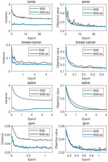
Figure 2: Comparison between SGD-as with SGD in logistic regression

We report the variances of the stochastic gradient in these two algorithms to check whether antithetic sampling can effectively reduce the variance, and evaluate the algorithms’ performance by objective value $f(w_{t})$ on training data. By comparing variance with the objective value, we can observe the impacts of variance on the algorithms’ performance.

Figure 2 summarizes the experiment results on logistic regression, and Figure 3 summarizes the results on SVM. According to the left column in each figures, we can observe that the variance of SGD-as is significantly smaller than that of SGD with uniform sampling, especially in the beginning of the iterations. This demonstrates the effectiveness of the proposed strategy to reduce the variance of the unbiased stochastic gradient estimators. In each figure, the right column shows the primal objective value of SGD-as in comparison to that of SGD with uniform sampling. We can observe that SGD-as converges faster and is much more stable than SGD. Since both algorithms iterate from $w=0$ and adopt the same step size in each iteration, this observation again implies that our antithetic sampling stratified sampling strategy is more effective to reduce the variance of stochastic gradient. For a certain dataset, we can see as the number of iterations increases, although the variance remains stable, the jitter of the convergence curve is slowing down. This is due to the decreasing step size weakens the impacts of variance. This is also the reason why SGD with the decreasing step size can converge in the presence of variance.

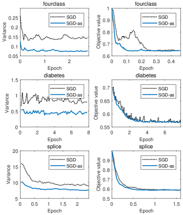
Figure 3: Comparison between SGD-as with SGD in SVM.

6 Conclusion

This paper studied antithetic sampling to reduce the variance for Stochastic Gradient Descent method. We considered the specific binary classification problems in detail. For some common binary classification problems, such as logistic regression and SVM, we proposed the fixed antithetic sampling strategy, which is practical and efficient. Promising empirical results validated the effectiveness of our technique.

References

- Allen-Zhu et al. [2016] Zeyuan Allen-Zhu, Yang Yuan, and Karthik Sridharan. Exploiting the structure: Stochastic gradient methods using raw clusters. In Advances in Neural Information Processing Systems 29, pages 1642–1650. Curran Associates, Inc., 2016.
- Allen-Zhu [2017] Zeyuan Allen-Zhu. Natasha 2: Faster non-convex optimization than sgd. arXiv preprint arXiv:1708.08694, 2017.
- Aly [2005] Mohamed Aly. Survey on multiclass classification methods. Neural Netw, 19:1–9, 2005.
- Bottou et al. [2016] Léon Bottou, Frank E. Curtis, and Jorge Nocedal. Optimization Methods for Large-Scale Machine Learning. arXiv:1606.04838 [cs, math, stat], 2016.
- Csiba et al. [2015] Dominik Csiba, Zheng Qu, and Peter Richtárik. Stochastic dual coordinate ascent with adaptive probabilities. In Proceedings of the 32nd International Conference on Machine Learning (ICML-15), pages 674–683, 2015.
- Defazio et al. [2014] Aaron Defazio, Francis Bach, and Simon Lacoste-Julien. Saga: A fast incremental gradient method with support for non-strongly convex composite objectives. In Advances in Neural Information Processing Systems 27, pages 1646–1654. Curran Associates, Inc., 2014.
- Duchi et al. [2010] John C Duchi, Shai Shalev-Shwartz, Yoram Singer, and Ambuj Tewari. Composite objective mirror descent. In COLT, pages 14–26, 2010.
- Johnson and Zhang [2013] Rie Johnson and Tong Zhang. Accelerating stochastic gradient descent using predictive variance reduction. In Advances in neural information processing systems, pages 315–323, 2013.
- Owen [2013] Art B. Owen. Monte Carlo theory, methods and examples. 2013.
- Robbins and Monro [1951] Herbert Robbins and Sutton Monro. A stochastic approximation method. The annals of mathematical statistics, pages 400–407, 1951.
- Ross [2013] Sheldon Ross. Chapter 9 - variance reduction techniques. In Sheldon Ross, editor, Simulation (Fifth Edition), pages 153 – 231. Academic Press, fifth edition edition, 2013.
- Shalev-Shwartz and Zhang [2013] Shai Shalev-Shwartz and Tong Zhang. Stochastic dual coordinate ascent methods for regularized loss minimization. Journal of Machine Learning Research, 14(Feb):567–599, 2013.
- Shalev-Shwartz et al. [2007] Shai Shalev-Shwartz, Yoram Singer, and Nathan Srebro. Pegasos: Primal estimated sub-gradient solver for svm. In Proceedings of the 24th International Conference on Machine Learning, ICML ’07, pages 807–814, New York, NY, USA, 2007. ACM.
- Shamir and Zhang [2013] Ohad Shamir and Tong Zhang. Stochastic gradient descent for non-smooth optimization: Convergence results and optimal averaging schemes. In International Conference on Machine Learning, pages 71–79, 2013.
- Shen et al. [2016] Zebang Shen, Hui Qian, Tengfei Zhou, and Tongzhou Mu. Adaptive variance reducing for stochastic gradient descent. In Proceedings of the Twenty-Fifth International Joint Conference on Artificial Intelligence, IJCAI’16, pages 1990–1996. AAAI Press, 2016.
- Stich et al. [2017] Sebastian U Stich, Anant Raj, and Martin Jaggi. Safe adaptive importance sampling. In I. Guyon, U. V. Luxburg, S. Bengio, H. Wallach, R. Fergus, S. Vishwanathan, and R. Garnett, editors, Advances in Neural Information Processing Systems 30, pages 4384–4394. Curran Associates, Inc., 2017.
- Wang et al. [2013] Chong Wang, Xi Chen, Alexander J Smola, and Eric P Xing. Variance reduction for stochastic gradient optimization. In C. J. C. Burges, L. Bottou, M. Welling, Z. Ghahramani, and K. Q. Weinberger, editors, Advances in Neural Information Processing Systems 26, pages 181–189. Curran Associates, Inc., 2013.
- Xiao and Zhang [2014] Lin Xiao and Tong Zhang. A proximal stochastic gradient method with progressive variance reduction. SIAM Journal on Optimization, 24(4):2057–2075, 2014.
- Zhao and Zhang [2014] Peilin Zhao and Tong Zhang. Accelerating minibatch stochastic gradient descent using stratified sampling. arXiv preprint arXiv:1405.3080, 2014.
- Zhao and Zhang [2015] Peilin Zhao and Tong Zhang. Stochastic optimization with importance sampling for regularized loss minimization. In Proceedings of the 32nd International Conference on Machine Learning (ICML-15), pages 1–9, 2015.
- Zhu [2016] Rong Zhu. Gradient-based sampling: An adaptive importance sampling for least-squares. In D. D. Lee, M. Sugiyama, U. V. Luxburg, I. Guyon, and R. Garnett, editors, Advances in Neural Information Processing Systems 29, pages 406–414. Curran Associates, Inc., 2016.