Anomalous diffusion in random dynamical systems

Abstract

Consider a chaotic dynamical system generating Brownian motion-like diffusion. Consider a second, non-chaotic system in which all particles localize. Let a particle experience a random combination of both systems by sampling between them in time. What type of diffusion is exhibited by this random dynamical system? We show that the resulting dynamics can generate anomalous diffusion, where in contrast to Brownian normal diffusion the mean square displacement of an ensemble of particles increases nonlinearly in time. Randomly mixing simple deterministic walks on the line we find anomalous dynamics characterised by ageing, weak ergodicity breaking, breaking of self-averaging and infinite invariant densities. This result holds for general types of noise and for perturbing nonlinear dynamics in bifurcation scenarios.

Many diffusion processes in nature and society were found to behave profoundly different from Brownian motion, which describes the random-looking flickering of a tracer particle in a fluid Shlesinger et al. (1993); Klafter et al. (1996); Klages et al. (2008); Metzler et al. (2014); Höfling and Franosch (2013); Meroz and Sokolov (2015); Viswanathan et al. (2011); Zaburdaev et al. (2015). Brownian dynamics provided a long-standing powerful paradigm to understand spreading in terms of normal diffusion, where the mean square displacement (MSD) of an ensemble of particles increases linearly in the long time limit, $\langle x^{2}\rangle\sim t^{\alpha}$ with $\alpha=1$. Anomalous diffusion is characterized by an exponent $\alpha\neq 1$ Shlesinger et al. (1993); Klafter et al. (1996); Klages et al. (2008); Metzler et al. (2014). Subdiffusion with $\alpha<1$ is commonly encountered in crowded environments as, e.g., for organelles moving in biological cells and single-file diffusion in nanoporous material Höfling and Franosch (2013); Meroz and Sokolov (2015). Superdiffusion with $\alpha>1$ is displayed by a variety of other systems, like animals searching for food and light propagating through disordered matter Viswanathan et al. (2011); Zaburdaev et al. (2015).

Experimental data exhibiting anomalous diffusion is often modelled successfully by advanced concepts of stochastic theory, most notably subdiffusive continuous time random walks, superdiffusive Lévy walks, generalized Langevin equations, or fractional Fokker-Planck equations Shlesinger et al. (1993); Klafter et al. (1996); Klages et al. (2008); Höfling and Franosch (2013); Meroz and Sokolov (2015); Viswanathan et al. (2011); Zaburdaev et al. (2015); Metzler et al. (2014). In these stochastic models the mechanisms generating anomalous diffusion are put in by hand on a coarse grained level, either via non-Gaussian probability distributions or via power law memory kernels. While this stochastic approach to anomalous diffusion has matured impressively, anomalous diffusion in deterministic dynamical systems is yet poorly understood. In nonlinear deterministic equations of motion there are only few mechanisms known to generate anomalous diffusion Klages et al. (2008): stickiness of orbits to KAM tori in Hamiltonian dynamics Zacherl et al. (1986); Shlesinger et al. (1993); Klafter et al. (1996); Zaslavsky (2002), marginally unstable fixed points in dissipative Pomeau-Manneville-like maps Geisel and Thomae (1984); Zumofen and Klafter (1993); Barkai (2003); Korabel et al. (2005, 2007) and non-trivial topologies exhibited by polygonal billiards Klages (2007). In this Letter we introduce a simple hybrid system at the interface between deterministic and stochastic dynamics. We show that it yields another generic mechanism for anomalous diffusion based on stochastic chaos in random dynamical systems Faranda et al. (2017); Sato et al. (2019). This sheds new light on the microscopic origin of anomalous dynamics. Similar models have been used to understand the convection of particles in flowing fluids Yu et al. (1990) including fractal clustering Wilkinson et al. (2003) and path coalescence Wilkinson and Mehlig (2003), the localisation transition in continuum percolation problems Höfling et al. (2006), intermittency in nonlinear electronic circuits Hammer et al. (1994) and random attractors in stochastic climate dynamics Chekroun et al. (2011). Accordingly, we expect fruitful applications of our approach to these problems.

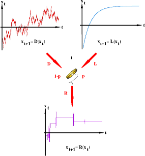
Figure 1: Diffusion generated by a random dynamical system. The three time series in space-time plots display the position $x_{t}\in\mathbb{R}$ of a point particle at discrete time $t\in\mathbb{N}$. The trajectory in the upper left is generated by the equation of motion $x_{t+1}=D(x_{t})$ using a deterministic dynamical system $D$ that yields normal diffusion. The trajectory in the upper right is from $x_{t+1}=L(x_{t})$ for a deterministic dynamical system $L$ where all particles localize in space. The random dynamical system $R$ mixes these two types of dynamics at time $t$ based on flipping a biased coin: The position $x_{t+1}$ of the particle at the next time $t+1$ is determined by choosing with probability $1-p$ the diffusive system $D$ while $L$ is picked with probability $p$. The trajectory generated by $x_{t+1}=R(x_{t})$ displays intermittency, where long regular phases alternate randomly with irregular-looking, chaotic motion.

Figure 1 gives our recipe to combine two deterministic dynamical systems $D$ and $L$ randomly in time. Here $D$ generates normal diffusion while $L$ yields localization of particles. We sample randomly between both systems with probability $p$ of choosing $L$ at discrete time step $t\in\mathbb{N}$, respectively probability $1-p$ of chooosing $D$. For $p=0$ we thus recover the dynamics of $D$ while for $p=1$ we obtain the one of $L$. This implies that there must exist a transition between these two different dynamics under variation of $p$. Our central question is: For $0<p<1$, what type of diffusive dynamics emerges in the resulting random dynamical system $R$? Here we model deterministic diffusion by chaotic random walks on the line Fujisaka and Grossmann (1982); Geisel and Nierwetberg (1982); Schell et al. (1982); Klages (2007) defined by the equation of motion $x_{t+1}=M_{a}(x_{t})$, where

$$M_{a}(x)=\left\{\begin{array}[]{r@{\quad,\quad}l}ax&0\leq x<\frac{1}{2}\\ ax+1-a&\frac{1}{2}\leq x<1\end{array}\right.\>,\>a>0\>,$$ (1)

is a piecewise linear map lifted onto $\mathbb{R}$ by $M_{a}(x+1)=M_{a}(x)+1$, cf. the inset in Fig. 2(a). For $a>2$ this model exhibits normal diffusion with a Lyapunov exponent calculated to (see Sec. 1 in our Supplement sup , which includes Refs. Ott (1993); Robinson (1995); Alligood et al. (1997); Dorfman (1999); Klages (2007, 2017)) $\lambda(a)=\ln a$ Klages and Dorfman (1995, 1999); Groeneveld and Klages (2002); Klages (2007). The sample trajectory in the upper left of Fig. 1 was obtained from $D=M_{4}(x)$, where the dynamics is chaotic according to $\lambda(4)=\ln 4>0$. The trajectory in the upper right of Fig. 1 corresponds to $L=M_{1/2}(x)$, where the dynamics is non-chaotic due to $\lambda(1/2)=-\ln 2<0$. Here all particles contract onto stable fixed points at integer positions $x\in\mathbb{Z}$. For defining the random map $R$ the slope $a$ becomes an independent and identically distributed, multiplicative random variable: At any time step $t$ we choose for our map $R=M_{a}(x)$ with probability $p\in[0,1]$ the slope $a=1/2$ while with probability $1-p$ we pick $a=4$. The sequence of random slopes may or may not depend on the individual particle if we consider an ensemble of them Bódai et al. (2013), as we explore below. Random maps of this type are also called iterated function systems Barnsley (1988); Abbasi et al. (2018). They have been studied by both mathematicians and physicists in view of their measure-theoretic Pelikan (1984); Ashwin et al. (1998); Abbasi et al. (2018) and statistical physical properties Yu et al. (1990); Klages (2002); Lipowski et al. (2004); Bódai et al. (2013).

Figure 2: Mean square displacement (MSD) and waiting time distribution (WTD) for randomized deterministic diffusion. The two deterministic dynamical systems that are randomly sampled in time with probability $p$ by applying the recipe of Fig. 1 are illustrated in the inset of (a). All symbols are generated from computer simulations. (a) MSD $\langle x_{t}^{2}\rangle$ for $p=0.6,0.63,0.663,2/3,0.669,0.68,0.7$ (top to bottom) for an ensemble of particles, where each particle experiences a different random sequence. There is a characteristic transition between normal diffusion and localization via subdiffusion at a critical $p_{c}=2/3$. (b) MSD at $p_{c}$ by starting the computations after different ageing times $t_{a}=0,10^{2},10^{3},10^{4}$ (top to bottom). The MSD displays ageing similar to analytical results from continuous time random walk (CTRW) theory Barkai (2003) (bold lines). (c) WTD $\eta(t)$ at $p_{c}$ for particles leaving a unit interval at the same ageing times $t_{a}$ as in (b). The bold lines are again analytical results from CTRW theory Barkai (2003). (d) MSD at the critical probability $p_{c}$ for different types of averaging over the random variable. For the straight black line with matching symbols each particle experiences a different random sequence (called uncommon noise), cf. Fig. 2(a). The other four lines depict MSDs obtained from applying the same sequence of random variables to all particles (called common noise). In these four cases the MSD becomes a random variable breaking self-averaging.

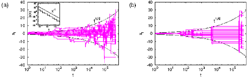
Figure 3: Subdiffusion for different types of randomness. (a) Sample trajectories at $p_{c}$ corresponding to 30 different initial conditions with uncommon noise. (b) Same as (a) with common noise. The envelopes in (a) and (b) correspond to the subdiffusive spreading for uncommon noise shown in Fig. 2(d). (b) displays jump time synchronization of all particles. The inset in (a) yields in double-logarithmic plot the infinite invariant density within a unit cell for uncommon noise for the map $R\;\mbox{mod 1}$.

One can show straightforwardly that the Lyapunov exponent $\lambda(p)$ of the random map $R$ is zero at probability $p_{c}=2/3$ sup . Since $\lambda(p)>0$ for $p<p_{c}$ the map $R$ should generate normal diffusion in this regime while $p>p_{c}$ with $\lambda(p)<0$ should lead to localization for long times. In Fig. 2 we test this conjecture by comparing numerical with analytical results. For our simulations we used $\sim 10^{5}$ iterations of $R$ with $\sim 10^{5}$ initial points, which were distributed randomly and uniformly in the unit interval $[0,1)$. Here each particle experienced a different sequence of random slopes. We used an arbitrary precision algorithm with up to $10^{10000}$ decimal digits. Figure 2(a) depicts the MSD $\langle x^{2}_{t}\rangle$ under variation of $p$ by confirming the diffusion scenario conjectured above. However, passing through $p_{c}$ the dynamics displays a subtle transition: Right at $p_{c}$ we obtain long-time subdiffusion, $\langle x^{2}(t)\rangle\sim t^{1/2}$, while around $p_{c}$ this dynamics survives for long transient times. Figures 2(b) and (c) reveal that right at $p_{c}$ $R$ exhibits ageing Bouchaud (1992); Metzler (2015) in both the MSD and the waiting time distribution (WTD). The latter is the probability distribution $\eta(t)$ of the times $t$ it takes a particle to escape from a unit interval of $R$. In both (b) and (c) there is good agreement with analytical results from continuous time random walk (CTRW) theory for long times, $\langle x_{t}^{2}\rangle\sim(t+t_{a})^{\alpha}-t_{a}^{\alpha}$ and $\eta(t)\sim t_{a}^{\alpha}/[(t+t_{a})t^{\alpha}]$, where $t_{a}$ is the ageing time Barkai (2003). This theory furthermore predicts that for long times a WTD of $\eta(t)\sim t^{-\gamma}$ implies a MSD of $\langle x^{2}(t)\rangle\sim t^{\gamma-1}$ Geisel and Thomae (1984); Zumofen and Klafter (1993); Barkai (2003); Korabel et al. (2005, 2007). For $R$ this relation is fulfilled with $\gamma=3/2$. An exponent of the WTD of $3/2$ yields a diverging mean waiting time. This as well as the existence of ageing imply weak ergodicity breaking of the dynamics Bouchaud (1992); Bel and Barkai (2005); Metzler (2015).

However, our map $R$ generates dynamics that goes beyond conventional CTRW theory. This becomes apparent by looking at different types of averaging over the random variables shown in Fig. 2(d): While in Fig. 2(a)-(c) each particle experienced a different sequence of random slopes, as reproduced by the straight line with matching symbols for the MSD in Fig. 2(d), for all the other MSDs in (d) the corresponding random sequences are the same for all particles. Accordingly, we call the former type of randomness uncommon noise, the latter common noise. Crucially, while in Fig. 2(a), based on uncommon noise, the MSD is well-defined for all $p$, Fig. 2(d) shows that for common noise sequences it becomes a random variable at $p_{c}$ in the long time limit that completely depends on the random squence chosen. This bears strong similarity to what is called breaking of self-averaging for random walks in quenched disordered environments Bouchaud and Georges (1990), which also implies weak ergodicity breaking Dentz et al. (2016).

Figure 3 displays space-time plots of 30 trajectories starting at different initial points for (a) uncommon noise and (b) common noise. While in (a) the different trajectories look rather irregular yielding a spreading front that matches to the subdiffusion depicted in Fig. 2(d) for uncommon noise, (b) shows ‘temporal clustering’ in the form of jump time synchronization, i.e., all particles eventually jump from unit cell to unit cell at the same time step. This matches to the fact that the MSD does not converge for common noise as seen in Fig. 2(d). The inset in (a) represents the invariant density of the map $R\;\mbox{mod 1}$, i.e., within a unit cell, with uncommon noise. We see that it decays on average like $\rho(x)\sim x^{-1}$. This result and the stepwise structure of $\rho(x)$ are in agreement with analytical calculations Pelikan (1984); Ashwin et al. (1998). At zero Lyapunov exponent uncommon noise thus leads to a weak spatial clustering Wilkinson et al. (2003) and path coalescence Wilkinson and Mehlig (2003) of particles at integer positions $x\in\mathbb{Z}$. In contrast, for common noise an invariant density does not exist, and we do not find any spatial clustering.

We now explore the origin of this type of anomalous dynamics in terms of dynamical systems theory. As exemplified by the trajectory shown at the bottom of Fig. 1, around $p_{c}$ the dynamics of $R$ is intermittent Bénichou et al. (2011) meaning long regular phases alternate randomly with irregular-looking, chaotic motion. A paradigmatic intermittent dynamical system is the Pomeau-Manneville map $P_{z,b}(x)=x+bx^{z}\>,\>b\geq 1\>,\>x\in[-1/2,1/2)$. Defining its equation of motion in the same way as for $M_{a}$ above it generates subdiffusion characterized by a MSD and a WTD that in suitable scaling limits match to the predictions of CTRW theory with $\gamma=z/(z-1)$ Geisel and Thomae (1984); Zumofen and Klafter (1993); Korabel et al. (2007). As shown above, for the map $R$ CTRW theory correctly predicts the relation between the long-time MSD and the WTD by using $\gamma=3/2$. Trying to understand the random map $R$ in terms of $P_{z,b}$ thus suggests to choose $z=3$. One should now compare the invariant densities $\rho(x)$ of the two maps mod 1: For $P_{z,b}\;\mbox{mod 1}$ it is known that $\rho(x)\sim x^{1-z}\>,\>x\gg 0$, which for $z\geq 2$ becomes a non-normalizable, infinite invariant density Thaler (1983); Korabel and Barkai (2009). But for $z=3$ this yields $\rho(x)\sim x^{-2}$ while for $R\;\mbox{mod 1}$ we have $\rho(x)\sim x^{-1}$, see the inset of Fig. 3(b) iid . Hence, the intermittency displayed by $R$ is not of Pomeau-Manneville type but of a fundamentally different microscopic dynamical origin. This might relate to deviations between CTRW theory, which on a coarse-grained level works well for the Pomeau-Manneville map, and our numerical results for $R$ on short time scales in the MSD and the WTD of Fig. 2. It would be interesting to further explore such differences, e.g., by the approach outlined in Ref. Albers and Radons (2013).

However, there is another type of intermittency in dynamical systems that is profoundly different from Pomeau-Manneville dynamics, called on-off intermittency Pikovsky (1984); Fujisaka and Yamada (1985, 1986); Pikovsky and Grassberger (1991); Platt et al. (1993); Heagy et al. (1994). It was first reported for two-dimensional coupled maps

$$x_{t+1} = (1-\epsilon)f(x_{t})+\epsilon f(y_{t})$$

$$y_{t+1} = (1-\epsilon)f(y_{t})+\epsilon f(x_{t})\quad,$$ (2)

where $x_{t+1}=f(x_{t})$ is chaotic with positive Lyapunov exponent and $\epsilon\in[0,1]$ Pikovsky (1984); Fujisaka and Yamada (1985). When $\epsilon$ is large, the possibly chaotic dynamics is trapped on the synchronization manifold $x_{t}=y_{t}$. By decreasing $\epsilon$ to a critical parameter $\epsilon=\epsilon^{*}$ trajectories start to escape from this manifold into the full two-dimensional space. This is called a blowout bifurcation and the associated intermittency on-off intermittency Ott and Sommerer (1994). In subsequent works Eqs. (2) were boiled down to more specific two-dimensional maps Pikovsky (1984); Pikovsky and Grassberger (1991); Fujisaka and Yamada (1986); Yu et al. (1990); Platt et al. (1993); Heagy et al. (1994); Hata and Miyazaki (1997); Ashwin et al. (1998). The simplest ones are piecewise linear Platt et al. (1993); Hata and Miyazaki (1997); Ashwin et al. (1998), such as Ashwin et al. (1998)

$$x_{t+1} = \left\{\begin{array}[]{cc}ax_{t}&(x_{t}<1\>,\>0\leq y_{t}\leq p)\\ \frac{1}{a}x_{t}&(x_{t}<1\>,\>p<y_{t}\leq 1)\\ 1+b(1-x_{t})&(x_{t}\geq 1)\end{array}\right.$$ (6)

$$y_{t+1} = \left\{\begin{array}[]{cc}\frac{y_{t}}{p}&(0\leq y_{t}\leq p)\\ \frac{y_{t}-p}{1-p}&(p<y_{t}\leq 1)\quad,\end{array}\right.$$ (9)

with symmetry $y\to-y$ and parameters $a>0,b\in\mathbb{R},p\in(0,1)$. Due to its skew product form this system can be understood as a one-dimensional map $x_{t+1}=f(x_{t})$ with multiplicative randomness generated by $y_{t+1}=g(y_{t})$ Pikovsky (1984); Pikovsky and Grassberger (1991); Fujisaka and Yamada (1986); Hata and Miyazaki (1997); Yu et al. (1990); Heagy et al. (1994). In a next step one might replace the deterministic chaotic dynamics of $y_{t}$ by stochastic noise. If we now consider the dynamics of $x_{t}$ in Eqs. (9) on the unit interval only by choosing $a=2$, taking the map mod 1 and choosing dichotomic noise, we obtain a simple piecewise linear map with multiplicative randomness that is qualitatively identical to our model $R\;\mbox{mod 1}$ Pelikan (1984); Yu et al. (1990); Ashwin et al. (1998). For this class of systems it has been shown numerically and analytically that at a critical $p_{c}$ the invariant density of $x=x_{t}$ decays like $\rho(x)\sim x^{-1}$ Pikovsky and Grassberger (1991); Fujisaka and Yamada (1985); Heagy et al. (1994); Hata and Miyazaki (1997); Ashwin et al. (1998); Harada et al. (1999); Miyazaki et al. (2001) and that a suitably defined waiting time distribution between chaotic ‘bursts’ obeys $\eta(t)\sim t^{-3/2}$ Heagy et al. (1994); Hata and Miyazaki (1997); Ashwin et al. (1998); Harada et al. (1999); Miyazaki et al. (2001). In Refs. Harada et al. (1999); Miyazaki et al. (2001) different diffusive models driven by on-off intermittency have been studied, and for two of them Miyazaki et al. (2001) subdiffusion with a MSD of $\langle x^{2}(t)\rangle\sim t^{1/2}$ has been obtained by matching simulation results to CTRW theory. We thus conclude that our model $R$ exhibits anomalous diffusion generated by on-off intermittency. We emphasize, however, that the mechanism underlying our model depicted in Fig. 1 is more general than this particular type of intermittent dynamics.

In order to check for the generality of our results, in the Supplement sup we first replace the dichotomic noise by physically more realistic continuous noise distributions choosing 1. uniform noise on a bounded interval, and 2. a non-uniform unbounded log-normal distribution. Figures 1 and 2 in Secs. 2 and 3 of sup , respectively, show that our mechanism is very robust under variation of the type of noise. We may thus conjecture that our scenario of subdiffusion generated by random maps holds for any generic type of noise. We also tested whether the strong localisation due to contraction onto a stable fixed point can be replaced by a weaker chaotic localisation to a subregion in phase space. However, in this case the transition between diffusive and localised dynamics is entirely different without displaying any subdiffusion, cf. Fig. 3 in Sec. 4 of sup . As a general principle, one must thus mix expansion with contraction to generate anomalous dynamics. Finally, in Sec. 5 of sup we study a simple nonlinear map that exhibits different types of diffusion in different parameter regions of a bifurcation scenario generating chaotic and periodic windows. Randomizing this map according to Fig. 1 yields again subdiffusion with a MSD of $\langle x_{t}^{2}\rangle\sim t^{1/2}$ and a WTD of $\eta(t)\sim t^{-3/2}$, cf. Fig. 4 in sup which includes Refs Bak et al. (1985); Korabel and Klages (2002, 2004). This demonstrates that the basic mechanism generating anomalous diffusion which we propose is also robust in a nonlinear setting.

In summary, we have shown that anomalous dynamics emerges if we randomly mix chaotic diffusion and non-chaotic localisation with a sampling probability yielding a zero Lyapunov exponent of the randomized dynamics. Interestingly, our basic mechanism bears similarity with the famous problem of a protein searching for a target at a DNA strand Berg et al. (1981): Here the protein randomly switches between (normal) diffusion in the bulk of the cell and moving along the DNA. This is called facilitated diffusion, as the random switching between different modes may decrease the average time to find a target Berg et al. (1981); Meroz et al. (2012); Bauer et al. (2012). We are not aware, however, that for this problem any emergence of anomalous diffusion as an effective dynamics representing the whole diffusion process has been discussed. Along these lines, one might speculate that using our framework for combining normal diffusion with constant velocity scanning Meroz et al. (2012) could yield a kind of Lévy walk Zaburdaev et al. (2015), which poses an interesting open problem.

Supplemental Material

Appendix A 1. Calculation of the Lyapunov exponent for random maps

For one-dimensional maps $M(x)$ obeying the deterministic equation of motion $x_{t+1}=M(x_{t})$ the local Lyapunov exponent is defined by Ott (1993); Robinson (1995); Alligood et al. (1997); Dorfman (1999); Klages (2007, 2017)

$$\lambda(x)=\lim_{t\to\infty}\frac{1}{t}\sum_{k=0}^{t-1}\ln|M^{\prime}(x_{k})|\quad,$$ (S1)

where $M^{\prime}(x)$ denotes the derivative of the map. By definition here the Lyapunov exponent $\lambda$ depends on the initial condition $x=x_{0}$ of the map, hence it is called local. Eq. (S1) represents a time average along the trajectory $\{x_{0},x_{1},\ldots,x_{k},\ldots,x_{t-1}\}$ of the map. If the map is ergodic the dependence on initial conditions will disappear Dorfman (1999); Klages (2007, 2017). For the piecewise linear map $M_{a}(x)$ defined by Eq. (1) in the main text we have that $M_{a}^{\prime}(x)=a$, hence $\lambda(a)=\ln a$ as noted in the main text on p.1.

We now apply Eq. (S1) to calculate the Lyapunov exponent for our random maps $R=M_{a}(x)$ as defined on p.1 and 2 in the main text, where $M_{a}(x)$ is again the piecewise linear map given by Eq. (1) in the main text. Therein the slope $a$ becomes a random variable drawn from a probability distribution $\chi(\xi)\>,\>a=\xi$, at any time step $t$, $a=a_{t}$. We first choose for $\chi$ dichotomic noise, where $a$ is sampled independently and identically distributed with probability $p\in[0,1]$ from $a=a_{loc}$ and with probability $1-p$ from $a=a_{exp}$. Feeding this information into Eq. (S1) we obtain

$$\lambda_{dich} = \lim_{t\to\infty}\left(\frac{t_{loc}}{t}\ln a_{loc}+\frac{t_{exp}}{t}\ln a_{exp}\right)$$ (S2)

$$= p\ln a_{loc}+(1-p)\ln a_{exp}\quad,$$

where $t_{loc}$ and $t_{exp}$ yield respective numbers of events out of a total of $t$ time steps for which the particle experiences the contracting and thus localising, respectively the expanding map Dorfman (1999). In the long time limit these fractions are identical with the corresponding sampling probabilities $p$ and $1-p$ leading to our final result. Note that in our piecewise linear map $R=M_{a}(x)$ all particles are exposed to the same uniform slope $a$ irrespective of initial conditions, hence $\lambda_{dich}=\lambda_{dich}(x)$.

From this equation we now calculate the critical sampling probability $p_{c}$ at which $\lambda_{dich}=0$ by choosing $a_{loc}=1/2$ and $a_{exp}=4$ as in the main text, which defines our first model. It follows

$$0=p\ln 1/2+(1-p)\ln 4\quad,$$ (S3)

which is solved to $p_{c}=2/3$ as stated on p.2 in the main text.

By observing that dichotomic noise is defined by the probability distribution

$$\chi_{dich}(\xi)=p\delta(\xi-a_{loc})+(1-p)\delta(\xi-a_{exp})$$ (S4)

we can rewrite Eq. (S2) more generally as

$$\lambda_{dich}=\int_{a_{loc}-\epsilon}^{a_{exp}+\epsilon}d\xi\>\chi_{dich}(\xi)\ln|\xi|$$ (S5)

with $0<\epsilon\ll 1$. From the above line of arguments it follows that for an arbitrary noise distribution $\chi(\xi)\>,\>\xi\in I$ we can calculate the Lyapunov exponent $\lambda_{\chi}$ of a random dynamical system $x_{t+1}=R(\xi_{t},x_{t})$ with map

$$R(\xi,x)=\left\{\begin{array}[]{ll}\xi x&0\leq x<\frac{1}{2}\\ \xi(x-1)+1&\frac{1}{2}\leq x<1\\ \end{array}\right.$$ (S8)

lifted onto the whole real line according to $R(x+1)=R(x)+1$ by

$$\lambda_{\chi}=\int_{I}d\xi\>\chi(\xi)\ln|\xi|\quad.$$ (S9)

Equations (S5),(S9) thus express the Lyapunov exponent of a random map $R$ by ensemble averages over the corresponding noise distributions instead of time averages along trajectories, which more generally presupposes ergodicity of the dynamics Dorfman (1999); Klages (2007, 2017). For maps that are more complicated than our piecewise linear case $M_{a}(x)$ Eq. (1) in the main text, calculating $\lambda_{\chi}$ will require integration over the full invariant density $\rho(x,\eta)$ of the random map, which can be a very non-trivial object Sato et al. (2019).

Appendix B 2. Random map with uniform distribution of slopes

We now consider a second model that is more general than the one defined by dichotomic noise. For this purpose we sample the slopes of the piecewise linear map Eq. (S8) from noise $\chi(\xi)$ uniformly distributed over an interval $\xi\in I=[a,b]\>,a>0$, that is, we choose

$$\xi\sim\chi_{unif}(\xi)=\frac{1}{b-a}\quad.$$ (S10)

For this model the Lyapunov exponent can be calculated from Eq. (S9) to

$$\lambda_{unif}=\int_{a}^{b}d\xi\>\frac{1}{b-a}\ln\xi=b\log b-b-(a\log a-a)\quad.$$ (S11)

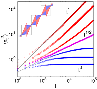
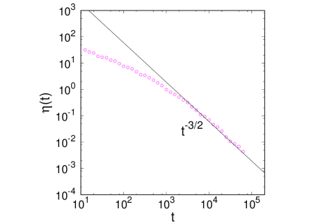
Supplementary Figure S1: Mean square displacement (MSD) and waiting time distribution (WTD) for the random map Eq. (S8) where the slopes are sampled from the uniform noise distribution Eq. (S10); see the inset on the left for an illustration. All symbols in the plots are generated from computer simulations. (left) MSD $\langle x_{t}^{2}\rangle$ for $b=2.5,2.45,2.38,2.36384,2.35,2.33,2.3$ (top to bottom) for an ensemble of particles, where each particle experiences a different random sequence. In complete analogy to Fig. 2(a) of the main text there is a characteristic transition between normal diffusion and localization via subdiffusion at a critical $b_{c}\simeq 2.36384$. (right) The WTD $\eta(t)$ at $b_{c}\simeq 2.36384$ showing a power law with exponent $-3/2$, cp. with Fig. 2(c) in the main text.

Choosing $a=0.1$ and keeping it fixed by varying the upper bound $b$, we obtain the critical parameter $b_{c}$ at which $\lambda_{unif}=0$ to $b_{c}\simeq 2.36384$. As for dichotomic noise we expect the resulting dynamics at $b_{c}$ to be subdiffusive, which is confirmed in Fig. S1. We conclude that our main result of subdiffusion in a random map is robust against generalising the noise distribution from a dichotomic one to uniform noise on a bounded interval.

Appendix C 3. Random map with log-normal distribution of slopes

Our third model is defined by sampling the slopes in the random map Eq. (S8) from a log-normal distribution,

$$\xi\sim\chi_{logn}(\xi)=\mbox{Lognormal($\mu$,1)}=\frac{1}{\xi\sqrt{2\pi}}\exp\left(-\frac{(\ln\xi-\mu)^{2}}{2}\right)\quad.$$ (S12)

The Lyapunov exponent can again be calculated from Eq. (S9) to

$$\lambda_{logn}=\int_{0}^{\infty}d\xi\>\frac{1}{\xi\sqrt{2\pi}}\exp\left(-\frac{(\ln\xi-\mu)^{2}}{2}\right)\ln\xi=\mu.$$ (S13)

For $\lambda_{logn}=0$ this yields trivially a critical parameter value of $\mu_{c}=0$ at which we expect the random map to generate subdiffusion. This is indeed confirmed in Fig. S2. We conclude that our main result of subdiffusion in a random map is also robust against generalising the noise distribution from uniform noise on a bounded interval to non-uniform noise on an unbounded interval.

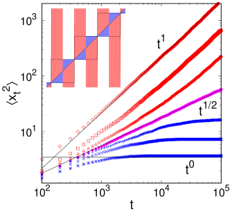
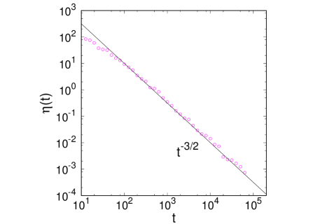
Supplementary Figure S2: MSD and WTD for the random map Eq. (S8) where the slopes are sampled from the log-normal distribution Eq. (S12); see the inset on the left for an illustration. All symbols in the plots are generated from computer simulations. (left) MSD $\langle x_{t}^{2}\rangle$ for $\mu=0.1,0.03,0.01,0,-0.07,-0.015,-0.03=$ (top to bottom) for an ensemble of particles, where each particle experiences a different random sequence. In complete analogy to Fig. 2(a) of the main text there is a characteristic transition between normal diffusion and localization via subdiffusion at a critical $\mu=0$. (right) The WTD $\eta(t)$ at $\mu=0$ showing a power law with exponent $-3/2$, cp. with Fig. 2(c) in the main text.

Appendix D 4. Random map with chaotic trapping

We now investigate whether the vanishing of the Lyapunov exponent exploited in the examples studied above is really necessary for having subdiffusion in our random maps. For this purpose we introduce a fourth model which is similar to our very first model Eqs. (S4),(S8) but for which we choose two slopes at which the corresponding deterministic maps are both expanding, $a_{loc}=3/2$ and $a_{exp}=4$. Note that for $a_{loc}=3/2$ the deterministic map Eq. (1) in the main text has a positive Lyapunov exponent $\lambda(3/2)=\ln 3/2$, see our calculation at the beginning of Sec. 1. Nevertheless, this map does not generate any long-time diffusion, since particles cannot escape from any unit interval due to the fact that the map does not exceed the unit interval. Hence these sets are trivially decoupled by generating chaotic trapping of particles on any unit interval.

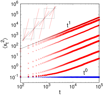
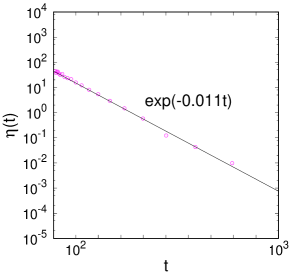
Supplementary Figure S3: MSD and WTD for the random map Eq. (S8) where the slopes are sampled from the dichotomic distribution Eq. (S4) with slopes $a_{loc}=3/2$ and $a_{exp}=4$; see the inset on the left for an illustration. Thus, in contrast to the map used for the corresponding results presented in Fig. 2 of the main text here the localisation is not due to contraction onto a stable fixed point but the dynamics remains chaotic on a bounded interval; see the text for further explanations. (left) MSD $\langle x_{t}^{2}\rangle$ for $p=0.0,0.5,0.9,0.99,0.995,0.9995,0.9999,1.0$ (top to bottom) for an ensemble of particles, where each particle experiences a different random sequence. In marked contrast to Fig. 2 of the main text, Fig. S1 and Fig. S2 above there is no characteristic transition between normal diffusion and localization via subdiffusion. (right) The WTD $\eta(t)$ at $p=0.99$ showing an exponential distribution, which is again in sharp contrast to the corresponding power law WTDs in the three figures mentioned above.

Figure S3 demonstrates that for this purely chaotic model there is no transition between normal diffusion and localisation via subdiffusion. In marked contrast to all our previous models we see that for $p>0$ the map always generates normal diffusion in the long time limit. Instead of subdiffusion the MSD displays longer and longer transients for shorter times at which diffusion is more and more slowed down when approaching the strictly localised dynamics at $p=1$. This numerical finding is confirmed by a WTD that is exponential even very close to the localisation value at $p=1$ as also shown in Fig. S3. It is in fact well known that for chaotic dynamical systems characterised by a positive Lyapunov exponent the WTD is always exponential while for non-chaotic systems exhibiting regular dynamics it decays as a power law Bauer and Bertsch (1990); Gaspard (1998). For an exact analytical calculation of the exponential WTD in an open version of the deterministic map Eq. (1) (main text) we refer to Refs. Ott (1993); Dorfman (1999); Klages (2017). To explicitly calculate the WTDs for this and our other random maps, possibly along these lines, in order to quantitatively confirm our numerical results from first principles remains an interesting open problem. We thus conclude that the condition of having a zero Lyapunov exponent is indispensable for observing subdiffusion in these random maps. This is deeply rooted in a mechanism yielding anomalous diffusion that requires an intricate interplay between contracting and expanding dynamics mixed in time.

Appendix E 5. Random nonlinear map

We finally test whether the observed subdiffusion in random maps also persists in nonlinear maps. As a fifth model we thus replace the map $M_{a}(x)$ Eq. (1) in the main text by the climbing sine map,

$$C_{c}(x)=x+c\sin(2\pi x)\>,\>x\in\mathbb{R}\quad,$$ (S14)

sketched in the inset of Fig. S4(b) Schell et al. (1982). This map can be derived from discretizing a driven nonlinear pendulum equation in time Bak et al. (1985) thus representing a much more general class of nonlinear dynamics than piecewise linear maps. It was found that $C_{c}$ displays three different regimes of diffusion under parameter variation with an exponent of the MSD of $\alpha=0$, $1$ or $2$ Korabel and Klages (2002, 2004). These regimes correspond to different parameter regions in the map’s bifurcation diagram reproduced in Fig. S4(a): $\alpha=1$ occurs in the chaotic regions while $\alpha=0$ and $2$ match to two different classes of periodic windows, where all particles either converge onto attracting localized periodic orbits, or onto ballistic ones.

Supplementary Figure S4: Subdiffusion in the random climbing sine map. (a) The bifurcation diagram of the climbing sine map depicted in the inset of (b) Korabel and Klages (2002, 2004). The two arrows denote the two specific parameter values $c_{1}=0.8$ and $c_{2}=0.2$ chosen with probability $1-p$, respectively $p$, to generate a random dynamical system from this map as explained in the text. (b) MSD at the critical probability $p_{c}\simeq 0.505702$ where the random map’s Lyapunov exponent is approximately zero. The symbols are from simulations, the line is a fit based on CTRW theory. The MSD clearly exhibits subdiffusion with exponent $1/2$. (c) The WTD for the same $p_{c}$ showing a power law with exponent $-3/2$ as predicted by CTRW theory; symbols and lines are as in (b).

Figures S4(b) and (c) show numerical results for the MSD and the WTD of the climbing sine map randomized by using the scheme of Fig. 1 in the main text. That is, with probability $1-p$ we choose the parameter $c_{1}=0.8$ sampling the chaotic region while with probability $p$ we draw from the attractive periodic orbit case at $c_{2}=0.2$. Both figures display results for the critical probability $p_{c}\simeq 0.505702$, where the map’s Lyapunov exponent is approximately zero. One can clearly see excellent matching of the exponents $\sim t^{1/2}$ for the MSD and $\sim t^{-3/2}$ for the WTD as predicted by conventional CTRW theory, cf. Fig. 2 in the main text. Hence, the basic mechanism that we propose to generate anomalous diffusion due to randomization of deterministic dynamics is also robust for a generic nonlinear map.

References

- Ott (1993) E. Ott, Chaos in Dynamical Systems (Cambridge University Press, Cambridge, 1993).
- Robinson (1995) C. Robinson, Dynamical Systems (CRC Press, London, 1995).
- Alligood et al. (1997) K.T. Alligood, T.S. Sauer, and J.A. Yorke, Chaos - An introduction to dynamical systems (Springer, New York, 1997).
- Dorfman (1999) J.R. Dorfman, An introduction to chaos in nonequilibrium statistical mechanics (Cambridge University Press, Cambridge, 1999).
- Klages (2007) R. Klages (2007), lecture notes, see http://www.maths.qmul.ac.uk/klages/teaching/mas424.
- Klages (2017) R. Klages, in Dynamical and complex systems, edited by S. Bullet, T. Fearn, and F. Smith (World Scientific, Singapore, 2017), vol. 5 of LTCC Advanced Mathematics Serie, pp. 1–40.
- Sato et al. (2019) Y. Sato, T. S. Doan, J. S. W. Lamb, and M. Rasmussen (2019), preprint arXiv:1811.03994.
- Bauer and Bertsch (1990) W. Bauer and G. F. Bertsch, Phys. Rev. Lett. 65, 2213 (1990).
- Gaspard (1998) P. Gaspard, Chaos, scattering, and statistical mechanics (Cambridge University Press, Cambridge, 1998).
- Schell et al. (1982) M. Schell, S. Fraser, and R. Kapral, Phys. Rev. A 26, 504 (1982).
- Bak et al. (1985) P. Bak, T. Bohr, and M.H. Jensen, Physica Scripta T9, 531 (1985).
- Korabel and Klages (2002) N. Korabel and R. Klages, Phys. Rev. Lett. 89, 214102 (2002).
- Korabel and Klages (2004) N. Korabel and R. Klages, Physica D 187, 66 (2004).