Asymptotic approximations for the close evaluation of double-layer potentials

Abstract

When using the boundary integral equation method to solve a boundary value problem, the evaluation of the solution near the boundary is challenging to compute because the layer potentials that represent the solution are nearly-singular integrals. To address this close evaluation problem, we apply an asymptotic analysis of these nearly singular integrals and obtain an asymptotic approximation. We derive the asymptotic approximation for the case of the double-layer potential in two and three dimensions, representing the solution of the interior Dirichlet problem for Laplace’s equation. By doing so, we obtain an asymptotic approximation given by the Dirichlet data at the boundary point nearest to the interior evaluation point plus a nonlocal correction. We present numerical methods to compute this asymptotic approximation, and we demonstrate the efficiency and accuracy of the asymptotic approximation through several examples. These examples show that the asymptotic approximation is useful as it accurately approximates the close evaluation of the double-layer potential while requiring only modest computational resources.

Keywords: Asymptotic approximation, close evaluation problem, potential theory, boundary integral equations.

1 Introduction

The close evaluation problem refers to the non-uniform error produced by high-order quadrature rules used in boundary integral equation methods. In particular, the close evaluation problem occurs when evaluating layer potentials at evaluation points close to the boundary. These high-order quadrature rules attain spectral accuracy when computing the solution, represented by layer potentials, far from the boundary whereas they incur a very large error when computing the solution close to the boundary. It is well understood that this growth in error is due to the fact that the integrand of the layer potentials become increasingly peaked as the point of evaluation approaches the boundary. In fact, when the distance between the evaluation point and its closest boundary point is smaller than the distance between quadrature points on the boundary for a fixed-order quadrature rule, the quadrature points do not adequately resolve the peak of the integrand and therefore produce an $O(1)$ error.

Accurate evaluations of layer potentials close to the boundary of the domain are needed for a wide range of applications, including the modeling of swimming micro-organisms, droplet suspensions, and blood cells in Stokes flow [41, 8, 31, 22], and to predict accurate measurements of the electromagnetic near-field in the field of plasmonics [30] for nano-antennas [3, 34] and sensors [33, 39].

Several computational methods have been developed to address this close evaluation problem. Schwab and Wendland [40] have developed a boundary extraction method based on a Taylor series expansion of the layer potentials. Beale and Lai [10] have developed a method that first regularizes the nearly singular kernel of the layer potential and then adds corrections for both the discretization and the regularization. Beale et al. [11] have extended the regularization method to three-dimensional problems. Helsing and Ojala [18] developed a method that combines a globally compensated quadrature rule and interpolation to achieve very accurate results over all regions of the domain. Barnett [9] has used surrogate local expansions with centers placed near, but not on, the boundary. Klöckner et al. [27] introduced Quadrature By Expansion (QBX), which uses expansions about accurate evaluation points far away from the boundary to compute accurate evaluations close to it. There have been several subsequent studies of QBX [15, 1, 38, 43, 2] that have extended its use and characterized its behavior.

Recently, the authors have applied asymptotic analysis to study the close evaluation problem. For two-dimensional problems, the authors developed a method that used matched asymptotic expansions for the kernel of the layer potential [12]. In that method, the asymptotic expansion that captures the peaked behavior of the kernel (namely, the peaked behavior of the integrand of the layer potential) can be integrated exactly and the relatively smooth remainder is integrated numerically, resulting in a highly accurate method. For three-dimensional problems, the authors have developed a simple, three-step method for computing layer potentials [13]. This method involves first rotating the spherical coordinate system used to compute the layer potential so that the boundary point at which the integrand becomes singular is aligned with the north pole. By studying the asymptotic behavior of the integral, they found that integration with respect to the azimuthal angle is a natural averaging operation that regularizes the integral thereby allowing for a high-order quadrature rule to be used for the integral with respect to the polar angle. This numerical method was shown to achieve an error that decays quadratically with the distance to the boundary provided that the underlying boundary integral equation for the density is sufficiently resolved.

In this work, we carry out a complete asymptotic analysis of the double-layer potential for the interior Dirichlet problem for Laplace’s equation in two and three dimensions. By doing so, we derive asymptotic approximations for the close evaluation of the double-layer potential. These asymptotic approximations provide valuable insight into the inherent challenges of the close evaluation problem and an explicit method to address it. We find that the leading-order asymptotic behavior of the double-layer potential in the close evaluation limit is given by the Dirichlet data at the boundary point closest to the evaluation point plus a nonlocal correction. It is the nonlocal correction that has made the close evaluation problem challenging to address. Since this asymptotic analysis explicitly finds this nonlocal correction, we are able to develop a simple and accurate numerical method to compute the double-layer potential and thus, address the close evaluation problem systematically. We compute several numerical examples using the asymptotic approximations to evaluate their efficacy and accuracy.

The asymptotic analysis used here to study the close evaluation problem also provides valuable insight (and useful asymptotic approximations) for other problems. In particular there is an interesting connection with forward-peaked scattering in radiative transfer, which is used to describe the multiple scattering of light [14, 20]. Forward-peaked scattering is an important problem for several applications, and is challenging to study. We draw this connection and apply the asymptotic analysis developed in this paper to forward-peaked scattering in radiative transfer.

The remainder of this paper is as follows. We precisely define the close evaluation problem for the double-layer potential in Section 2. We compute the leading-order asymptotic behavior of the double-layer potential in two and three dimensions in Sections 3 and 4, respectively. We describe numerical methods to evaluate the asymptotic approximations for the close evaluation of the double-layer potential in Section 5. We give several examples demonstrating the accuracy of this numerical method in Section 6. Section 7 describes the connection between the close evaluation problem and forward-peaked scattering in radiative transfer. Section 8 gives our conclusions. The Appendix provides details of the computations for the three-dimensional case: Appendix A gives details of how we rotate spherical integrals and Appendix B gives a useful derivation of the spherical Laplacian.

2 Close evaluation of the double-layer potential

Consider a simply connected, open set, denoted by $D\subset\mathbb{R}^{n}$ with $n=2,3$, with an analytic close boundary, $B$, and let $\bar{D}=D\cup B$. Given some smooth data $f$, we write the function $u\in C^{2}(D)\cap C^{1}(\bar{D})$ satisfying the interior Dirichlet problem,

$$\varDelta u=0\quad\text{in $D$},$$ (2.1a)

$$u=f\quad\text{on $B$},$$ (2.1b)

as the double-layer potential,

$$u(x)=\frac{1}{2^{n-1}\pi}\int_{B}\frac{\nu_{y}\cdot(x-y)}{|x-y|^{n}}\mu(y)\mathrm{d}\sigma_{y},\quad x\in D,\quad n=2,3.$$ (2.2)

Here, $\nu_{y}$ denotes the unit outward normal at $y\in B$, $\mathrm{d}\sigma_{y}$ denotes the boundary element, and $\mu$, the density, is a continuous function. This double-layer potential satisfies the following jump relation [17],

$$\lim_{\begin{subarray}{c}x\to y^{\star}\in B\\ x\in D\end{subarray}}u(x)=u(y^{\star})-\frac{1}{2}\mu(y^{\star}).$$ (2.3)

By requiring that $u$ satisfies (2.1), we find that, in light of jump relation (2.3), $\mu$ must satisfy

$$\frac{1}{2^{n-1}\pi}\int_{B}\frac{\nu_{y}\cdot(y^{\star}-y)}{|y^{\star}-y|^{n}}\mu(y)\mathrm{d}\sigma_{y}-\frac{1}{2}\mu(y^{\star})=f(y^{\star}),\quad y^{\star}\in B,$$ (2.4)

the boundary integral equation for $\mu$.

Here, we seek to evaluate (2.2) at points close to the boundary. To define a close evaluation point precisely, let $0<\varepsilon\ll 1$ denote a small, dimensionless parameter, and consider

$$x=y^{\star}-\varepsilon\ell\nu^{\star},$$ (2.5)

with $y^{\star}\in B$ denoting the closest point to $x$ on the boundary, $\nu^{\star}$ denoting the unit, outward normal at $y^{\star}$, and $\ell$ denoting a characteristic length of the problem such as the signed (2D) or mean (3D) curvature at $y^{\star}$ (see Fig. 1).

Figure 1: Sketch of the quantities introduced in (2.5) to study evaluation points close to the boundary in 2D (left) and in 3D (right).

Because the solution of (2.1) continuously approaches its boundary data from within $D$, we write

$$u(x)=u(y^{\star}-\varepsilon\ell\nu^{\star})=f(y^{\star})+\varepsilon U(y^{\star};\varepsilon).$$ (2.6)

To determine an expression for $U$, we substitute (2.2) evaluated at (2.5) for $u(y^{\star}-\varepsilon\ell\nu^{\star})$ and (2.4) for $f(y^{\star})$ into (2.6), and find that

$$U(y^{\star};\varepsilon)=\varepsilon^{-1}\left[\frac{1}{2}\mu(y^{\star})+\frac{1}{2^{n-1}\pi}\int_{B}\left[\frac{\nu_{y}\cdot(y_{d}-\varepsilon\ell\nu^{\star})}{|y_{d}-\varepsilon\ell\nu^{\star}|^{n}}-\frac{\nu_{y}\cdot y_{d}}{|y_{d}|^{n}}\right]\mu(y)\mathrm{d}\sigma_{y}\right],$$ (2.7)

where we have introduced the notation, $y_{d}=y^{\star}-y$. Next, we make use of Gauss’ theorem [17]

$$\frac{1}{2^{n-1}\pi}\int_{B}\frac{\nu_{y}\cdot(x-y)}{|x-y|^{n}}\mathrm{d}\sigma_{y}=\begin{cases}-1&x\in D,\\ -\frac{1}{2}&x\in B,\\ \,\,\,\,0&x\not\in\bar{D},\end{cases}$$ (2.8)

to write

$$\frac{1}{2}\mu(y^{\star})=-\frac{1}{2^{n-1}\pi}\int_{B}\frac{\nu_{y}\cdot(y_{d}-\varepsilon\ell\nu^{\star})}{|y_{d}-\varepsilon\ell\nu^{\star}|^{n}}\mu(y^{\star})\mathrm{d}\sigma_{y}+\frac{1}{2^{n-1}\pi}\int_{B}\frac{\nu_{y}\cdot y_{d}}{|y_{d}|^{n}}\mu(y^{\star})\mathrm{d}\sigma_{y}.$$ (2.9)

Substituting (2.9) into (2.7) yields

$$U(y^{\star};\varepsilon)=\frac{1}{2^{n-1}\pi}\int_{B}\varepsilon^{-1}\left[\frac{\nu_{y}\cdot(y_{d}-\varepsilon\ell\nu^{\star})}{|y_{d}-\varepsilon\ell\nu^{\star}|^{n}}-\frac{\nu_{y}\cdot y_{d}}{|y_{d}|^{n}}\right][\mu(y)-\mu(y^{\star})]\mathrm{d}\sigma_{y}.$$ (2.10)

We seek to determine the asymptotic expansion of $U$ given in (2.10) in the limit as $\varepsilon\to 0^{+}$. To determine this asymptotic expansion, we make use of explicit parametrizations for $B$. Therefore, we consider the two and three-dimensional problems separately.

3 Asymptotic analysis in two dimensions

Suppose $B$ is an analytic, closed curve on the plane. For that case, we introduce the parameter $t\in[-\pi,\pi]$ such that $y=y(t)$ and $y^{\star}=y(0)$. In terms of this parameterization, (2.10) is given by

$$U(y^{\star};\varepsilon)=\frac{1}{2\pi}\int_{-\pi}^{\pi}\varepsilon^{-1}K(t;\varepsilon)[\tilde{\mu}(t)-\tilde{\mu}(0)]\mathrm{d}t,$$ (3.1)

with $\tilde{\mu}(t)=\mu(y(t))$, $\tilde{\mu}(0)=\mu(y(0))=\mu(y^{\star})$, and

$$K(t;\varepsilon)=\left[\frac{\tilde{\nu}(t)\cdot(y_{d}(t)-\varepsilon\ell\nu^{\star})}{|y_{d}(t)-\varepsilon\ell\nu^{\star}|^{2}}-\frac{\tilde{\nu}(t)\cdot y_{d}(t)}{|y_{d}(t)|^{2}}\right]J(t),$$ (3.2)

with $\tilde{\nu}(t)=\nu(y(t))$, $y_{d}(t)=y(0)-y(t)$, and $J(t)=|y^{\prime}(t)|$. Note that $\nu^{\star}=\tilde{\nu}(0)$.

To determine the asymptotic expansion for $U$, we introduce the small parameter $\delta$ satisfying $0<\varepsilon\ll\delta\ll 1$, and write

$$U(y^{\star};\varepsilon)=U^{\text{in}}(y^{\star};\varepsilon,\delta)+U^{\text{out}}(y^{\star};\varepsilon,\delta).$$ (3.3)

Here, the inner expansion, $U^{\text{in}}$, is given by

$$U^{\text{in}}(y^{\star};\varepsilon,\delta)=\frac{1}{2\pi}\int_{-\delta/2}^{\delta/2}\varepsilon^{-1}K(t;\varepsilon)\left[\tilde{\mu}(t)-\tilde{\mu}(0)\right]\mathrm{d}t,$$ (3.4)

and the outer expansion, $U^{\text{out}}$, is given by

$$U^{\text{out}}(y^{\star};\varepsilon,\delta)=\frac{1}{2\pi}\int_{-\pi}^{-\delta/2}\varepsilon^{-1}K(t;\varepsilon)\left[\tilde{\mu}(t)-\tilde{\mu}(0)\right]\mathrm{d}t+\frac{1}{2\pi}\int_{\delta/2}^{\pi}\varepsilon^{-1}K(t;\varepsilon)\left[\tilde{\mu}(t)-\tilde{\mu}(0)\right]\mathrm{d}t.$$ (3.5)

The inner expansion involves integration over a small portion of the boundary about $y^{\star}$, whereas the outer expansion involves integration over the remaining portion of the boundary.

We determine the leading-order asymptotic behaviors of $U^{\text{in}}$ and $U^{\text{out}}$ in the sections below. Then, we combine those results to obtain the asymptotic approximation for the double-layer potential in two dimensions, and discuss higher-order asymptotic approximations. We have developed a Mathematica notebook that contains the presented calculations, available in a GitHub repository [23].

3.1 Inner expansion

To determine the leading-order asymptotic behavior of $U^{\text{in}}$, we substitute $t=\varepsilon T$ into (3.4), and obtain

$$U^{\text{in}}(y^{\star};\varepsilon,\delta)=\frac{1}{2\pi}\int_{-\delta/2\varepsilon}^{\delta/2\varepsilon}K(\varepsilon T;\varepsilon)\left[\tilde{\mu}(\varepsilon T)-\tilde{\mu}(0)\right]\mathrm{d}T.$$ (3.6)

Recognizing that $\tilde{\nu}(\varepsilon T)=\nu^{\star}+O(\varepsilon)$ and $y_{d}(\varepsilon T)=-\varepsilon Ty^{\prime}(0)+O(\varepsilon^{2})$ with $\nu^{\star}\cdot y^{\prime}(0)=0$, we find that by expanding $K(\varepsilon T;\varepsilon)$ about $\varepsilon=0$ that

$$K(\varepsilon T;\varepsilon)=-\frac{\varepsilon^{-1}\ell J(0)}{T^{2}J^{2}(0)+\ell^{2}}+O(1).$$ (3.7)

Using the fact that this leading-order behavior is even in $T$, and expanding $\tilde{\mu}$ about $\varepsilon=0$, we can substitute into (3.6) to get, after expanding about $\delta=0$,

$$\begin{split}U^{\text{in}}&(y^{\star};\varepsilon,\delta)=\frac{1}{2\pi}\int_{-\delta/2\varepsilon}^{\delta/2\varepsilon}\left[-\frac{\varepsilon^{-1}\ell J(0)}{T^{2}J^{2}(0)+\ell^{2}}+O(1)\right]\left[\tilde{\mu}(\varepsilon T)-\tilde{\mu}(0)\right]\mathrm{d}T\\ &=\frac{1}{2\pi}\int_{0}^{\delta/2\varepsilon}\left[-\frac{\varepsilon^{-1}\ell J(0)}{T^{2}J^{2}(0)+\ell^{2}}+O(1)\right]\left[\tilde{\mu}(\varepsilon T)+\tilde{\mu}(-\varepsilon T)-2\tilde{\mu}(0)\right]\mathrm{d}T\\ &=\frac{1}{2\pi}\int_{0}^{\delta/2\varepsilon}\left[-\frac{\varepsilon^{-1}\ell J(0)}{T^{2}J^{2}(0)+\ell^{2}}+O(1)\right]\left[\varepsilon^{2}T^{2}\tilde{\mu}^{\prime\prime}(0)+O(\varepsilon^{4})\right]\mathrm{d}T\\ &=\frac{1}{2\pi}\int_{0}^{\delta/2\varepsilon}\left[-\frac{\varepsilon T^{2}\ell J(0)}{T^{2}J^{2}(0)+\ell^{2}}\tilde{\mu}^{\prime\prime}(0)+O(\varepsilon^{2})\right]\mathrm{d}T\\ &=-\frac{\delta\ell}{4\pi J(0)}\tilde{\mu}^{\prime\prime}(0)+O(\varepsilon).\end{split}$$ (3.8)

This result gives the leading-order asymptotic behavior of $U^{\text{in}}$.

3.2 Outer expansion

To determine the leading-order asymptotic behavior of $U^{\text{out}}$, we expand $K(t;\varepsilon)$ about $\varepsilon=0$ and find that $K(t;\varepsilon)=[\varepsilon K_{1}(t)+O(\varepsilon^{2})]J(t)$, with

$$K_{1}(t)=\ell\frac{2(\tilde{\nu}(t)\cdot y_{d}(t))(\nu^{\star}\cdot y_{d}(t))-\tilde{\nu}(t)\cdot\nu^{\star}|y_{d}(t)|^{2}}{|y_{d}(t)|^{4}}.$$ (3.9)

Substituting this expansion into (3.5), we find that

$$U^{\text{out}}(y^{\star};\varepsilon,\delta)=\frac{1}{2\pi}\int_{-\pi}^{-\delta/2}K_{1}(t)\left[\tilde{\mu}(t)-\tilde{\mu}(0)\right]J(t)\mathrm{d}t+\frac{1}{2\pi}\int_{\delta/2}^{\pi}K_{1}(t)\left[\tilde{\mu}(t)-\tilde{\mu}(0)\right]J(t)\mathrm{d}t+O(\varepsilon).$$ (3.10)

To eliminate $\delta$ from the integration limits, we rewrite (3.10) as

$$U^{\text{out}}(y^{\star};\varepsilon,\delta)=\frac{1}{2\pi}\int_{-\pi}^{\pi}K_{1}(t)\left[\tilde{\mu}(t)-\tilde{\mu}(0)\right]J(t)\mathrm{d}t-V^{\text{out}}(y^{\star};\varepsilon,\delta)+O(\varepsilon)$$ (3.11)

with

$$V^{\text{out}}(y^{\star};\varepsilon,\delta)=\frac{1}{2\pi}\int_{-\delta/2}^{\delta/2}K_{1}(t)\left[\tilde{\mu}(t)-\tilde{\mu}(0)\right]J(t)\mathrm{d}t.$$ (3.12)

To determine the leading-order behavior for $V^{\text{out}}$, we proceed exactly as in section 3.1. We substitute $t=\varepsilon T$ into (3.12) and obtain

$$V^{\text{out}}(y^{\star};\varepsilon,\delta)=\frac{1}{2\pi}\int_{-\delta/2\varepsilon}^{\delta/2\varepsilon}K_{1}(\varepsilon T)\left[\tilde{\mu}(\varepsilon T)-\tilde{\mu}(0)\right]J(\varepsilon T)\varepsilon\mathrm{d}T$$ (3.13)

Again, by recognizing that $\tilde{\nu}(\varepsilon T)=\nu^{\star}+O(\varepsilon)$ and $y_{d}(\varepsilon T)=-\varepsilon Ty^{\prime}(0)+O(\varepsilon^{2})$ with $\nu^{\star}\cdot y^{\prime}(0)=0$, we find that

$$K_{1}(\varepsilon T)=-\frac{\varepsilon^{-2}\ell}{T^{2}J^{2}(0)}+O(\varepsilon^{-1}).$$ (3.14)

Using the fact that this leading-order behavior is even in $T$, and that $J(\varepsilon T)=J(0)+O(\varepsilon)$, when we substitute it into (3.13), we find, after expanding about $\delta=0$, that

$$\begin{split}V^{\text{out}}&(y^{\star};\varepsilon,\delta)=\frac{1}{2\pi}\int_{-\delta/2\varepsilon}^{\delta/2\varepsilon}\left[-\frac{\varepsilon^{-2}\ell}{T^{2}J^{2}(0)}+O(\varepsilon^{-1})\right]\left[\tilde{\mu}(\varepsilon T)-\tilde{\mu}(0)\right]J(\varepsilon T)\varepsilon\mathrm{d}T\\ &=\frac{1}{2\pi}\int_{0}^{\delta/2\varepsilon}\left[-\frac{\varepsilon^{-2}\ell}{T^{2}J^{2}(0)}+O(\varepsilon^{-1})\right]\left[\tilde{\mu}(\varepsilon T)+\tilde{\mu}(-\varepsilon T)-2\tilde{\mu}(0)\right]\left[J(0)+O(\varepsilon)\right]\varepsilon\mathrm{d}T\\ &=\frac{1}{2\pi}\int_{0}^{\delta/2\varepsilon}\left[-\frac{\varepsilon^{-1}\ell}{T^{2}J(0)}+O(1)\right]\left[\varepsilon^{2}T^{2}\tilde{\mu}^{\prime\prime}(0)+O(\varepsilon^{4})\right]\mathrm{d}T\\ &=\frac{1}{2\pi}\int_{0}^{\delta/2\varepsilon}\left[-\frac{\varepsilon\ell}{J(0)}\tilde{\mu}^{\prime\prime}(0)+O(\varepsilon^{2})\right]\mathrm{d}T\\ &=-\frac{\delta\ell}{4\pi J(0)}\tilde{\mu}^{\prime\prime}(0)+O(\varepsilon).\end{split}$$ (3.15)

Substituting this result into (3.11), we find that the leading-order asymptotic behavior for $U^{\text{out}}$ is given by

$$U^{\text{out}}(y^{\star};\varepsilon,\delta)=\frac{1}{2\pi}\int_{-\pi}^{\pi}K_{1}(t)\left[\tilde{\mu}(t)-\tilde{\mu}(0)\right]J(t)\mathrm{d}t+\frac{\delta\ell}{4\pi J(0)}\tilde{\mu}^{\prime\prime}(0)+O(\varepsilon).$$ (3.16)

3.3 Two-dimensional asymptotic approximation

We obtain an asymptotic approximation for $U$ by summing the leading-order behaviors obtained for $U^{\text{in}}$ and $U^{\text{out}}$ given in (3.8) and (3.16), respectively. Substituting that result into (2.6), we obtain the following asymptotic approximation,

$$u(y^{\star}-\varepsilon\ell\nu^{\star})=f(y^{\star})+\varepsilon L_{1}[\mu]+O(\varepsilon^{2}),$$ (3.17)

with

$$L_{1}[\mu]=\frac{1}{2\pi}\int_{-\pi}^{\pi}K_{1}(t)\left[\tilde{\mu}(t)-\tilde{\mu}(0)\right]J(t)\mathrm{d}t,$$ (3.18)

where $K_{1}$ is given by (3.9). Naturally, the obtained asymptotic approximation doesn’t depend on the arbitrary parameter $\delta$.

Asymptotic approximation (3.17) gives an explicit approximation for the close evaluation of the double-layer potential in two dimensions. According to the asymptotic analysis, the error of this approximation is $O(\varepsilon^{2})$. It gives the double-layer potential as the Dirichlet data at the boundary point $y^{\star}$ closest to the evaluation point $x$ plus a nonlocal correction. This nonlocal correction is consistent with the fact that solutions to elliptic partial differential equations have a global dependence on their boundary data. The leading-order asymptotic expansion indicates that the nonlocal correction only comes from the outer expansion, and the inner expansion doesn’t contribute to the lower order terms.

3.4 Higher-order asymptotic approximations

By continuing on to higher order terms in the expansions for $U^{\text{in}}$ and $U^{\text{out}}$, we can obtain higher-order asymptotic approximations. This process will not be demonstrated here, because the calculations become unwieldy, details can be found in the developed Mathematica notebook [23]. The result from these calculations is

$$u(y^{\star}-\varepsilon\ell\nu^{\star})=f(y^{\star})+\varepsilon L_{1}[\mu]+\varepsilon^{2}\left[L_{2}[\mu]-\frac{\ell^{2}y^{\prime}(0)\cdot y^{\prime\prime}(0)}{4J^{4}(0)}\tilde{\mu}^{\prime}(0)+\frac{\ell^{2}}{4J^{2}(0)}\tilde{\mu}^{\prime\prime}(0)\right]+O(\varepsilon^{3}),$$ (3.19)

with $L_{1}[\mu]$ given in (3.18), and

$$L_{2}[\mu]=\frac{1}{2\pi}\int_{-\pi}^{\pi}K_{2}(t)\left[\tilde{\mu}(t)-\tilde{\mu}(0)\right]J(t)\mathrm{d}t,$$ (3.20)

where

$$K_{2}(t)=\ell^{2}\frac{(\nu\cdot y_{d})\left[4(\nu^{\star}\cdot y_{d})^{2}-|y_{d}|^{2}\right]-2|y_{d}|^{2}(\nu\cdot\nu^{\star})(\nu^{\star}\cdot y_{d})}{|y_{d}|^{6}}.$$ (3.21)

This asymptotic approximation has an error that is $O(\varepsilon^{3})$. In addition to nonlocal terms, this approximation includes local contributions made by first and second derivatives of the density, $\mu$, evaluated at the boundary point $y^{\star}$. The local contributions come from the inner expansion.

4 Asymptotic analysis in three dimensions

Suppose $B$ is an analytic, closed, and oriented surface. We introduce the parameters $s\in[0,\pi]$ and $t\in[-\pi,\pi]$ such that $y=y(s,t)$ and $y^{\star}=y(0,\cdot)$. In terms of this parameterization, (2.10) is given by

$$U(y^{\star};\varepsilon)=\frac{1}{4\pi}\int_{-\pi}^{\pi}\int_{0}^{\pi}\varepsilon^{-1}K(s,t;\varepsilon)\left[\tilde{\mu}(s,t)-\tilde{\mu}(0,\cdot)\right]\sin(s)\mathrm{d}s\mathrm{d}t,$$ (4.1)

with $\tilde{\mu}(s,t)=\mu(y(s,t))$, $\tilde{\mu}(0,\cdot)=\mu(y(0,\cdot))$, and

$$K(s,t;\varepsilon)=\left[\frac{\tilde{\nu}(s,t)\cdot(y_{d}(s,t)-\varepsilon\ell\nu^{\star})}{|y_{d}(s,t)-\varepsilon\ell\nu^{\star}|^{3}}-\frac{\tilde{\nu}(s,t)\cdot y_{d}(s,t)}{|y_{d}(s,t)|^{3}}\right]J(s,t),$$ (4.2)

with $\tilde{\nu}(s,t)=\nu_{y}$, $y_{d}(s,t)=y(0,\cdot)-y(s,t)$, $J(s,t)=|y_{s}(s,t)\times y_{t}(s,t)|/\sin(s)$. Note that $\nu^{\star}=\tilde{\nu}(0,\cdot)$.

Just as we have done for the two dimensional problem, we introduce the small parameter $\delta$ satisfying $0<\varepsilon\ll\delta\ll 1$, and write

$$U(y^{\star};\varepsilon)=U^{\text{in}}(y^{\star};\varepsilon,\delta)+U^{\text{out}}(y^{\star};\varepsilon,\delta).$$ (4.3)

Here, the inner expansion is given by

$$U^{\text{in}}(y^{\star};\varepsilon,\delta)=\frac{1}{4\pi}\int_{-\pi}^{\pi}\int_{0}^{\delta}\varepsilon^{-1}K(s,t;\varepsilon)\left[\tilde{\mu}(s,t)-\tilde{\mu}(0,\cdot)\right]\sin(s)\mathrm{d}s\mathrm{d}t,$$ (4.4)

and the outer expansion is given by

$$U^{\text{out}}(y^{\star};\varepsilon,\delta)=\frac{1}{4\pi}\int_{-\pi}^{\pi}\int_{\delta}^{\pi}\varepsilon^{-1}K(s,t;\varepsilon)\left[\tilde{\mu}(s,t)-\tilde{\mu}(0,\cdot)\right]\sin(s)\mathrm{d}s\mathrm{d}t.$$ (4.5)

Again, we determine the leading-order asymptotic behaviors for $U^{\text{in}}$ and $U^{\text{out}}$ separately. Then, we combine those results to obtain an asymptotic approximation for the close evaluation of the double-layer potential in three dimensions and discuss higher-order asymptotic approximations. Some details can be found in the developed Mathematica notebook available on GitHub [23].

4.1 Inner expansion

To find the leading-order asymptotic behavior of $U^{\text{in}}$, we substitute $s=\varepsilon S$ into (4.4), and obtain

$$U^{\text{in}}(y^{\star};\varepsilon,\delta)=\frac{1}{4\pi}\int_{-\pi}^{\pi}\int_{0}^{\delta/\varepsilon}K(\varepsilon S,t;\varepsilon)\left[\tilde{\mu}(\varepsilon S,t)-\tilde{\mu}(0,\cdot)\right]\sin(\varepsilon S)\mathrm{d}S\mathrm{d}t.$$ (4.6)

Recognizing that $\tilde{\nu}(\varepsilon S,t)=\nu^{\star}+O(\varepsilon)$, and $y_{d}(\varepsilon S,t)=-\varepsilon Sy_{s}(0,\cdot)+O(\varepsilon^{2})$ with the vector $y_{s}(0,\cdot)$ lying on the plane tangent to $B$ at $y^{\star}$, we find by expanding $K(\varepsilon S,t;\varepsilon)$ about $\varepsilon=0$ that

$$K(\varepsilon S,t;\varepsilon)=-\frac{\varepsilon^{-2}\ell J(0,\cdot)}{(S^{2}|y_{s}(0,\cdot)|^{2}+\ell^{2})^{3/2}}+O(\varepsilon^{-1}).$$ (4.7)

Since this leading-order asymptotic behavior for $K(\varepsilon S,t;\varepsilon)$ is independent of $t$, we write

$$U^{\text{in}}(y^{\star};\varepsilon,\delta)=\frac{1}{4\pi}\int_{0}^{\pi}\int_{0}^{\delta/\varepsilon}\left[-\frac{\varepsilon^{-2}\ell J(0,\cdot)}{(S^{2}|y_{s}(0,\cdot)|^{2}+\ell^{2})^{3/2}}+O(\varepsilon^{-1})\right]\\ \left[\tilde{\mu}(\varepsilon S,t)+\tilde{\mu}(\varepsilon S,t+\pi)-2\tilde{\mu}(0,\cdot)\right]\sin(\varepsilon S)\mathrm{d}S\mathrm{d}t.$$ (4.8)

Next, we use the regularity of $\tilde{\mu}$ over the north pole to substitute $\tilde{\mu}(\varepsilon S,t+\pi)=\tilde{\mu}(-\varepsilon S,t)$, so that

$$\begin{split}\tilde{\mu}(\varepsilon S,t)+\tilde{\mu}(\varepsilon S,t+\pi)-2\tilde{\mu}(0,\cdot)&=\tilde{\mu}(\varepsilon S,t)+\tilde{\mu}(-\varepsilon S,t)-2\tilde{\mu}(0,\cdot)\\ &=\varepsilon^{2}S^{2}\tilde{\mu}_{ss}(0,\cdot)+O(\varepsilon^{4}).\end{split}$$ (4.9)

Thus, we find after substituting (4.9) and $\sin(\varepsilon S)=\varepsilon S+O(\varepsilon^{3})$ into (4.8) that

$$\begin{split}U^{\text{in}}(y^{\star};\varepsilon,\delta)&=\frac{1}{4\pi}\int_{0}^{\pi}\int_{0}^{\delta/\varepsilon}\left[-\frac{\varepsilon S^{3}\ell J(0,\cdot)}{(S^{2}|y_{s}(0,\cdot)|^{2}+\ell^{2})^{3/2}}\tilde{\mu}_{ss}(0,\cdot)+O(\varepsilon^{2})\right]\mathrm{d}S\mathrm{d}t\\ &=-\frac{\ell J(0,\cdot)}{8}\varDelta_{S^{2}}\mu(y^{\star})\int_{0}^{\delta/\varepsilon}\left[\frac{\varepsilon S^{3}}{(S^{2}|y_{s}(0,\cdot)|^{2}+\ell^{2})^{3/2}}+O(\varepsilon^{2})\right]\mathrm{d}S,\end{split}$$ (4.10)

where we have used the fact that

$$\frac{1}{\pi}\int_{0}^{\pi}\tilde{\mu}_{ss}(0,\cdot)\mathrm{d}t=\frac{1}{2}\varDelta_{S^{2}}\mu(y^{\star}),$$ (4.11)

with $\varDelta_{S^{2}}\mu(y^{\star})$ denoting the spherical Laplacian of $\mu$ evaluated at $y^{\star}$ (see Appendix B). Furthermore, when expanding about $\delta=0$ we have

$$\int_{0}^{\delta/\varepsilon}\left[\frac{\varepsilon S^{3}}{(S^{2}|y_{s}(0,\cdot)|^{2}+\ell^{2})^{3/2}}+O(\varepsilon^{2})\right]\mathrm{d}S=\frac{\delta}{|y_{s}(0,\cdot)|^{3}}+O(\varepsilon),$$ (4.12)

we determine that

$$U^{\text{in}}(y^{\star};\varepsilon,\delta)=-\frac{\delta\ell J(0,\cdot)}{8|y_{s}(0,\cdot)|^{3}}\varDelta_{S^{2}}\mu(y^{\star})+O(\varepsilon).$$ (4.13)

This result gives the leading-order asymptotic behavior of $U^{\text{in}}$.

4.2 Outer expansion

To determine the leading-order asymptotic behavior of $U^{\text{out}}$, we expand $K(s,t;\varepsilon)$ about $\varepsilon=0$ and find $K(s,t;\varepsilon)=$ $\left[\varepsilon K_{1}(s,t)+O(\varepsilon^{2})\right]J(s,t)$, with

$$K_{1}(s,t)=\ell\frac{3(\tilde{\nu}(s,t)\cdot y_{d}(s,t))(\nu^{\star}\cdot y_{d}(s,t))-|y_{d}(s,t)|^{2}\tilde{\nu}(s,t)\cdot\nu^{\star}}{|y_{d}(s,t)|^{5}}.$$ (4.14)

Substituting this expansion into (4.5), we obtain

$$U^{\text{out}}(y^{\star};\varepsilon,\delta)=\frac{1}{4\pi}\int_{-\pi}^{\pi}\int_{\delta}^{\pi}K_{1}(s,t)\left[\tilde{\mu}(s,t)-\tilde{\mu}(0,\cdot)\right]J(s,t)\sin(s)\mathrm{d}s\mathrm{d}t+O(\varepsilon).$$ (4.15)

To eliminate $\delta$ as a limit of integration in (4.15), we write

$$U^{\text{out}}(y^{\star};\varepsilon,\delta)=\frac{1}{4\pi}\int_{-\pi}^{\pi}\int_{0}^{\pi}K_{1}(s,t)\left[\tilde{\mu}(s,t)-\tilde{\mu}(0,\cdot)\right]J(s,t)\sin(s)\mathrm{d}s\mathrm{d}t-V^{\text{out}}(y^{\star};\varepsilon,\delta)+O(\varepsilon),$$ (4.16)

with

$$V^{\text{out}}(y^{\star};\varepsilon,\delta)=\frac{1}{4\pi}\int_{-\pi}^{\pi}\int_{0}^{\delta}K_{1}(s,t)\left[\tilde{\mu}(s,t)-\tilde{\mu}(0,\cdot)\right]J(s,t)\sin(s)\mathrm{d}s\mathrm{d}t.$$ (4.17)

To determine the leading-order asymptotic behavior of $V^{\text{out}}(y^{\star};\varepsilon,\delta)$, we proceed as in section 4.1. We substitute $s=\varepsilon S$ into (4.17), and obtain

$$V^{\text{out}}(y^{\star};\varepsilon,\delta)=\frac{1}{4\pi}\int_{-\pi}^{\pi}\int_{0}^{\delta/\varepsilon}K_{1}(\varepsilon S,t)\left[\tilde{\mu}(\varepsilon S,t)-\tilde{\mu}(0,\cdot)\right]J(\varepsilon S,t)\sin(\varepsilon S)\varepsilon\mathrm{d}S\mathrm{d}t.$$ (4.18)

Recognizing that $\tilde{\nu}(\varepsilon S,t)=\nu^{\star}+O(\varepsilon)$, and $y_{d}(\varepsilon S,t)=-\varepsilon Sy_{s}(0,\cdot)+O(\varepsilon^{2})$ with the vector $y_{s}(0,\cdot)$ lying on the plane tangent to $B$ at $y^{\star}$, we find by expanding $K_{1}(\varepsilon S,t)$ about $\varepsilon=0$ that

$$K_{1}(\varepsilon S,t)=-\frac{\varepsilon^{-3}\ell}{S^{3}|y_{s}(0,\cdot)|^{3}}+O(\varepsilon^{-2}).$$ (4.19)

Since the leading-order behavior of $K_{1}$ is independent of $t$, we use (4.9), plus knowing that $J(\varepsilon S,t)=J(0,\cdot)+O(\varepsilon)$ and $\sin(\varepsilon S)=\varepsilon S+O(\varepsilon^{3})$ to obtain, after expanding about $\delta=0$

$$\begin{split}V^{\text{out}}(y^{\star};\varepsilon,\delta)&=\frac{1}{4\pi}\int_{0}^{\pi}\int_{0}^{\delta/\varepsilon}\left[-\frac{\varepsilon\ell J(0,\cdot)}{|y_{s}(0,\cdot)|^{3}}\tilde{\mu}_{ss}(0,\cdot)+O(\varepsilon^{2})\right]\mathrm{d}S\mathrm{d}t\\ &=-\frac{\delta\ell J(0,\cdot)}{8|y_{s}(0,\cdot)|^{3}}\varDelta_{S^{2}}\mu(y^{\star})+O(\varepsilon).\end{split}$$ (4.20)

Note that we have used (4.11) in the last step. Substituting this result into (4.16), we find that

$$U^{\text{out}}(y^{\star};\varepsilon,\delta)=\frac{1}{4\pi}\int_{-\pi}^{\pi}\int_{0}^{\pi}K_{1}(s,t)\left[\tilde{\mu}(s,t)-\tilde{\mu}(0,\cdot)\right]J(s,t)\sin(s)\mathrm{d}s\mathrm{d}t+\delta\frac{\ell J(0,\cdot)}{8|y_{s}(0,\cdot)|^{3}}\varDelta_{S^{2}}\mu(y^{\star})+O(\varepsilon).$$ (4.21)

This result gives the leading-order asymptotic behavior of $U^{\text{out}}$.

4.3 Three-dimensional asymptotic approximation

We obtain an asymptotic approximation for $U$ by summing the leading-order behaviors obtained for $U^{\text{in}}$ and $U^{\text{out}}$ given in (4.13) and (4.21), respectively. Substituting that result into (2.6), we obtain the following asymptotic approximation

$$u(y^{\star}-\varepsilon\ell\nu^{\star})=f(y^{\star})+\varepsilon L_{1}[\mu]+O(\varepsilon^{2}),$$ (4.22)

with

$$L_{1}[\mu]=\frac{1}{4\pi}\int_{-\pi}^{\pi}\int_{0}^{\pi}K_{1}(s,t)\left[\tilde{\mu}(s,t)-\tilde{\mu}(0,\cdot)\right]J(s,t)\sin(s)\mathrm{d}s\mathrm{d}t.$$ (4.23)

The structure of this asymptotic approximation for the close evaluation of the double-layer potential in three dimensions is exactly the same as what we found for the two-dimensional case: the leading-order asymptotic approximation is composed of the Dirichlet data and a non-local term coming from the outer expansion. Similarly, high-order asymptotic approximations could be obtained by continuing on to higher order terms in the expansions $U^{\text{in}}$ and $U^{\text{out}}$ after cumbersome calculations.

5 Numerical methods

Numerical methods to compute the asymptotic approximations for the close evaluation of the double-layer potential must be sufficiently accurate in comparison to $O(\varepsilon)$. Otherwise, the error made by the numerical method will dominate over the error of the asymptotic approximation. On the other hand, if the numerical method requires restrictively high resolution to compute the asymptotic approximation to sufficient accuracy, the numerical method suffers from the very issue of the close evaluation problem. In what follows, we describe numerical methods to compute the asymptotic approximations derived above at high accuracy with modest resolution requirements.

5.1 Two dimensions

Suppose we have parameterized $B$ by $y=y(\varphi)$ with $-\pi\leq\varphi\leq\pi$ with $y^{\star}=y(\varphi^{\star})$. For that case, we need to compute

$$\mathscr{U}_{1}(y^{\star})=\frac{1}{2\pi}\int_{-\pi}^{\pi}F_{1}(\varphi;\varphi^{\star})\mathrm{d}\varphi,$$ (5.1)

with

$$F_{1}(\varphi;\varphi^{\star})=K_{1}(\varphi)J(\varphi)\left[\tilde{\mu}(\varphi)-\tilde{\mu}(\varphi^{\star})\right],$$ (5.2)

where $K_{1}$ is given in (3.9). The function, $K_{1}$, is singular at $\varphi=\varphi^{\star}$. Consequently, applying a high order accurate numerical quadrature rule to compute $\mathscr{U}_{1}$ will be limited in its accuracy even though $F_{1}$ vanishes identically at $\varphi=\varphi^{\star}$ due to the factor of $\tilde{\mu}(\varphi)-\tilde{\mu}(\varphi^{\star})$. To improve the accuracy of a numerical evaluation of (5.1), we revisit the asymptotic expansion obtained for $V^{\text{out}}(y^{\star};\varepsilon,\delta)$ in (3.13)-(3.15). By rewriting that result for the present context, we find

$$\frac{1}{2\pi}\int_{-\delta/2}^{\delta/2}F_{1}(\varphi;\varphi^{\star})\mathrm{d}\varphi=-\frac{\delta}{4\pi}\frac{\ell\tilde{\mu}^{\prime\prime}(\varphi^{\star})}{J(\varphi^{\star})}+O(\varepsilon).$$ (5.3)

This result suggests the following method to compute $\mathscr{U}_{1}(y^{\star})$ numerically using the $N$-point periodic trapezoid rule (PTR). Suppose we are given the grid function, $\tilde{\mu}(\varphi_{j})$ for $j=1,\cdots,N$ with $\varphi_{j}=-\pi+2\pi(j-1)/N$, and suppose $\varphi^{\star}=\varphi_{k}$ is one of the quadrature points. We introduce the numerical approximation

$$\mathscr{U}_{1}(y^{\star})\approx U_{1}^{N}(y^{\star})=\frac{1}{N}\sum_{j\neq k}F_{1}(\varphi_{j};\varphi_{k})-\frac{\ell\tilde{\mu}^{\prime\prime}(\varphi_{k})}{2NJ(\varphi_{k})}.$$ (5.4)

where we have replaced the quadrature around $\varphi^{\star}$ with (5.3) where $\delta=2\pi/N$. We compute $\tilde{\mu}^{\prime\prime}(\varphi_{k})$ with spectral accuracy using Fast Fourier transform methods. Using this numerical approximation, we compute the $O(\varepsilon^{2})$ asymptotic approximation for the close evaluation of the double-layer potential in two dimensions through evaluation of

$$u(y^{\star}-\varepsilon\ell\nu^{\star})\approx f(y^{\star})+\varepsilon U_{1}^{N}(y^{\star})+O(\varepsilon^{2}).$$ (5.5)

To compute the $O(\varepsilon^{3})$ asymptotic approximation, in addition to $\mathscr{U}_{1}$, we need to compute

$$\mathscr{U}_{2}(y^{\star})=\frac{1}{2\pi}\int_{-\pi}^{\pi}F_{2}(\varphi;\varphi^{\star})\mathrm{d}\varphi$$ (5.6)

where

$$F_{2}(\varphi;\varphi^{\star})=K_{2}(\varphi)J(\varphi)\left[\tilde{\mu}(\varphi)-\tilde{\mu}(\varphi^{\star})\right],$$ (5.7)

and $K_{2}$ given in (3.21). By using the higher-order asymptotic expansion for $V^{\text{out}}$ (computed on the Mathematica notebook available on the GitHub repository [23]), we apply the same method used for $\mathscr{U}_{1}(y^{\star})$ and arrive at

$$\mathscr{U}_{2}(y^{\star})\approx U_{2}^{N}=\frac{1}{N}\sum_{j\neq k}F_{2}(\varphi_{j};\varphi_{k})-\frac{\ell^{2}\kappa^{\star}\tilde{\mu}^{\prime\prime}(\varphi_{k})}{4NJ(\varphi_{k})},$$ (5.8)

with $\kappa^{\star}$ denoting the signed curvature at $y^{\star}$. Using this numerical approximation, we compute the $O(\varepsilon^{3})$ asymptotic approximation for the close evaluation of the double-layer potential in two dimensions through evaluation of

$$u(y^{\star}-\varepsilon\ell\nu^{\star})\approx f(y^{\star})+\varepsilon U_{1}^{N}(y^{\star})+\varepsilon^{2}\left[U_{2}^{N}(y^{\star})-\frac{\ell^{2}y^{\prime}(\varphi^{\star})\cdot y^{\prime\prime}(\varphi^{\star})}{4J^{4}(\varphi^{\star})}\tilde{\mu}^{\prime}(\varphi^{\star})+\frac{\ell^{2}\tilde{\mu}^{\prime\prime}(\varphi^{\star})}{4J^{2}(\varphi^{\star})}\right]+O(\varepsilon^{3}).$$ (5.9)

Since the boundary is given, we are able to compute $y^{\prime}(\varphi)$ and $y^{\prime\prime}(\varphi)$, explicitly. We use Fast Fourier transform methods to compute $\tilde{\mu}^{\prime}(\varphi)$ and $\tilde{\mu}^{\prime\prime}(\varphi)$ with spectral accuracy.

5.2 Three dimensions

Suppose we have parameterized $B$ by $y=y(\theta,\varphi)$ with $\theta\in[0,\pi]$ and $\varphi\in[-\pi,\pi]$ with $y^{\star}=y(\theta^{\star},\varphi^{\star})$. For that case, we seek to compute

$$\mathscr{U}_{1}(y^{\star})=\frac{1}{4\pi}\int_{-\pi}^{\pi}\int_{0}^{\pi}F_{1}(\theta,\varphi;\theta^{\star},\varphi^{\star})\sin(\theta)\mathrm{d}\theta\mathrm{d}\varphi,$$ (5.10)

with

$$F_{1}(\theta,\varphi;\theta^{\star},\varphi^{\star})=K_{1}(\theta,\varphi)J(\theta,\varphi)\left[\tilde{\mu}(\theta,\varphi)-\tilde{\mu}(\theta^{\star},\varphi^{\star})\right],$$ (5.11)

where $K_{1}$ is given in (4.14). Just as with the two-dimensional case, the function $K_{1}$ is singular at $(\theta,\varphi)=(\theta^{\star},\varphi^{\star})$, so any attempt to apply a quadrature rule to compute $\mathscr{U}_{1}$ will be limited in its accuracy even though $F_{1}$ vanishes identically at $(\theta^{\star},\varphi^{\star})$ due to the factor of $\tilde{\mu}(\theta,\varphi)-\tilde{\mu}(\theta^{\star},\varphi^{\star})$.

To numerically evaluate (5.10), we apply a three-step method developed by the authors [13]. This method has been shown to be effective for computing the modified double-layer potential in three dimensions resulting from the subtraction method. We first rotate this integral to another spherical coordinate system in which $y^{\star}$ is aligned with the north pole. The details of this rotation are given in Appendix A and lead to $\theta=\theta(s,t)$ and $\varphi=\varphi(s,t)$ with $s\in[0,\pi]$ and $t\in[-\pi,\pi]$ where $\theta^{\star}=\theta(0,\cdot)$ and $\varphi^{\star}=\varphi(0,\cdot)$. We apply this rotation and find that

$$\mathscr{U}_{1}(y^{\star})=\frac{1}{4\pi}\int_{-\pi}^{\pi}\int_{0}^{\pi}\tilde{F}(s,t)\sin(s)\mathrm{d}s\mathrm{d}t,$$ (5.12)

with $\tilde{F}(s,t)=F_{1}(\theta(s,t),\varphi(s,t);\theta^{\star},\varphi^{\star})$. Now $\tilde{K}_{1}(\theta(s,t),\varphi(s,t))$ is singular at the north pole of this rotated coordinate system corresponding to $s=0$. To improve the accuracy of a numerical evaluation of (5.12), we revisit the asymptotic expansion obtained for $V^{\text{out}}(y^{\star};\varepsilon,\delta)$ in (4.20). By rewriting that result for the present context, we find

$$\frac{1}{2}\int_{0}^{\delta}\left[\frac{1}{2\pi}\int_{-\pi}^{\pi}\tilde{F}(s,t)\mathrm{d}t\right]\sin(s)\mathrm{d}s=\int_{0}^{\delta}\left[-\frac{\ell J(0,\cdot)}{8|y_{s}(0,\cdot)|^{3}}\varDelta_{S^{2}}\mu(y^{\star})\right]\mathrm{d}s+O(\varepsilon).$$ (5.13)

Suppose we compute

$$\bar{F}(s)=\frac{1}{2\pi}\int_{-\pi}^{\pi}\tilde{F}(s,t)\mathrm{d}t.$$ (5.14)

The result in (5.13) suggests that $\bar{F}(s)$ smoothly limits to a finite value as $s\to 0$. Although we could use this result to evaluate $\bar{F}(s)$ in a numerical quadrature scheme, it will suffice to consider an open quadrature rule for $s$ that does not include the point $s=0$ such as the Gauss-Legendre quadrature. This result suggests the following three-step method to compute $\mathscr{U}_{1}(y^{\star})$ numerically.

Let $t_{k}=-\pi+\pi(k-1)/N$ for $k=1,\cdots,2N$, and let $z_{j}$ and $w_{j}$ for $j=1,\cdots,N$ denote the $N$-point Gauss-Legendre quadrature abscissas and weights such that

$$\int_{-1}^{1}f(x)\mathrm{d}x\approx\sum_{j=1}^{N}f(z_{j})w_{j}.$$ (5.15)

We perform the mapping: $s_{j}=\pi(z_{j}+1)/2$ for $j=1,\cdots,N$, and make appropriate adjustments to the weights as will be shown below. For the first step, we rotate the spherical coordinate system so that $y^{\star}$ is aligned with its north pole as described in Appendix A. For the second step, we compute

$$\bar{F}(s_{j})\approx\bar{F}^{N}_{j}=\frac{1}{2N}\sum_{k=1}^{2N}\tilde{F}(s_{j},t_{k}),\quad j=1,\cdots,N.$$ (5.16)

For the third step, we compute the numerical approximation

$$\mathscr{U}_{1}(y^{\star})\approx U_{1}^{N}(y^{\star})=\frac{\pi}{4}\sum_{j=1}^{N}\bar{F}_{j}^{N}w_{j}.$$ (5.17)

In (5.17), a factor of $\pi/2$ is introduced to scale the quadrature weights due to the mapping from $z_{j}$ to $s_{j}$, and a factor of $1/2$ remains from the factor of $1/4\pi$ in (5.10).

Using the numerical approximation $U_{1}^{N}$, we compute the $O(\varepsilon^{2})$ asymptotic approximation for the close evaluation of the double-layer potential in three dimensions through evaluation of

$$u(y^{\star}-\varepsilon\ell\nu^{\star})\approx f(y^{\star})+\varepsilon U_{1}^{N}(y^{\star})+O(\varepsilon^{2}).$$ (5.18)

6 Numerical results

We present results that show the accuracy and efficiency of the asymptotic approximation and the corresponding numerical method for the close evaluation of the double-layer potential. For all of the examples shown, we prescribe Dirichlet data corresponding to a particular harmonic function. With that Dirichlet data, we solve the boundary integral equation (2.4) numerically to obtain the density, $\mu$. We use that density to compute the double-layer potential using different methods, for comparison. The results below show the error made in computing the harmonic function at close evaluation points. The Matlab codes used to compute all of the following examples are available in a GitHub repository [23].

6.1 Two dimensions

For the two-dimensional examples, we use the harmonic function,

$$u(x)=-\frac{1}{2\pi}\log|x-x_{0}|,$$ (6.1)

with $x_{0}\in\mathbb{R}^{2}\setminus\bar{D}$ and prescribe Dirichlet data by evaluating this function on the boundary. We solve the boundary integral equation (2.4) using the Nyström method with the $N$-point Periodic Trapezoid Rule (PTR) resulting in the numerical approximation for the density, $\tilde{\mu}_{j}\approx\tilde{\mu}(\varphi_{j})$ with $\varphi_{j}=-\pi+2(j-1)\pi/N$ for $j=1,\cdots,N$.

We compute the close evaluation of the double-layer potential at points, $x=y^{\star}-\varepsilon\nu^{\star}$, using the following four methods:

1. PTR method – Compute the double-layer potential,

   $$u(y^{\star}-\varepsilon\nu^{\star})=\frac{1}{2\pi}\int_{-\pi}^{\pi}\frac{\nu_{y}\cdot(y^{\star}-\varepsilon\nu^{\star}-y)}{|y^{\star}-\varepsilon\nu^{\star}-y|^{2}}\mu(y)\mathrm{d}\sigma_{y},$$

   using the same $N$-point PTR used to solve (2.4) .

2. Subtraction method – Compute the modified double-layer potential,

   $$u(y^{\star}-\varepsilon\nu^{\star})=-\mu(y^{\star})+\frac{1}{2\pi}\int_{-\pi}^{\pi}\frac{\nu_{y}\cdot(y^{\star}-\varepsilon\nu^{\star}-y)}{|y^{\star}-\varepsilon\nu^{\star}-y|^{2}}\left[\mu(y)-\mu(y^{\star})\right]\mathrm{d}\sigma_{y},$$

   using the same $N$-point PTR used to solve (2.4) and as in the first method.

3. $O(\varepsilon^{2})$ asymptotic approximation – Compute the $O(\varepsilon^{2})$ asymptotic approximation given by (3.17) using the new numerical method given in (5.5) using the same $N$-point PTR used to solve (2.4).

4. $O(\varepsilon^{3})$ asymptotic approximation – Compute the $O(\varepsilon^{3})$ asymptotic approximation given by (3.19) using the new numerical method given in (5.9) using the same $N$-point PTR used to solve (2.4).

We consider two different domains:

• A kite domain whose boundary is given by

  $$y(t)=(\cos t+0.65\cos 2t-0.65,1.5\sin t),\quad-\pi\leq t\leq\pi.$$ (6.2)

• A star domain whose boundary is given by

  $$y(t)=r(t)(\cos t,\sin t),\quad r(t)=1+0.3\cos 5t,\quad-\pi\leq t\leq\pi.$$ (6.3)

For both examples we pick $x_{0}=(1.85,1.65)$ which lies outside the domains. We consider $N$ fixed, here $N=128$, and study the dependence of the error on $\varepsilon$ as $\varepsilon\to 0$.

In Fig. 3 we show results for the kite domain. The error, using a $\log$ scale, is presented for each of the four methods described above. The results show that the PTR method exhibits an $O(1)$ error as $\varepsilon\to 0$. The subtraction method and the asymptotic approximations all show substantially smaller errors.

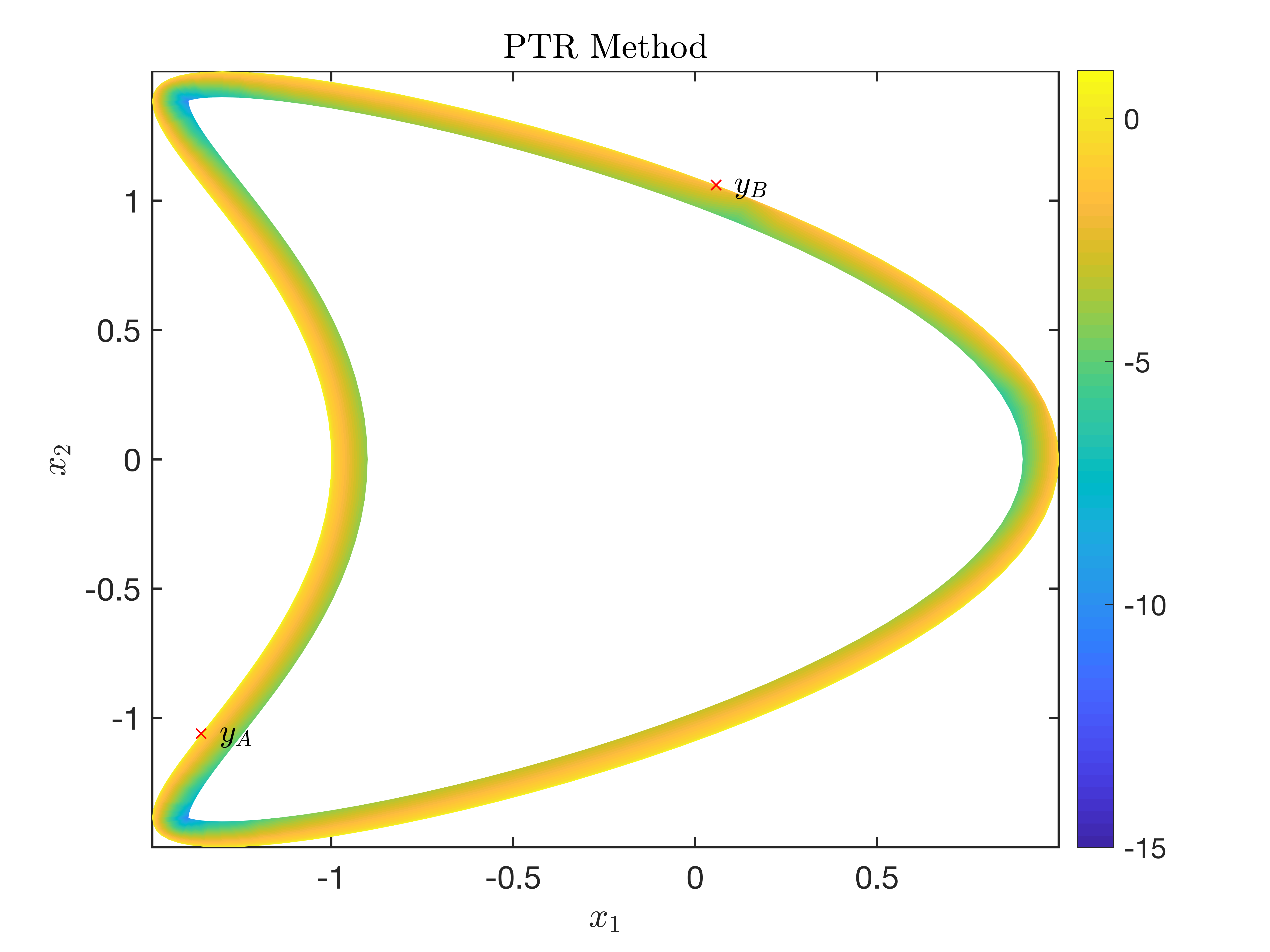
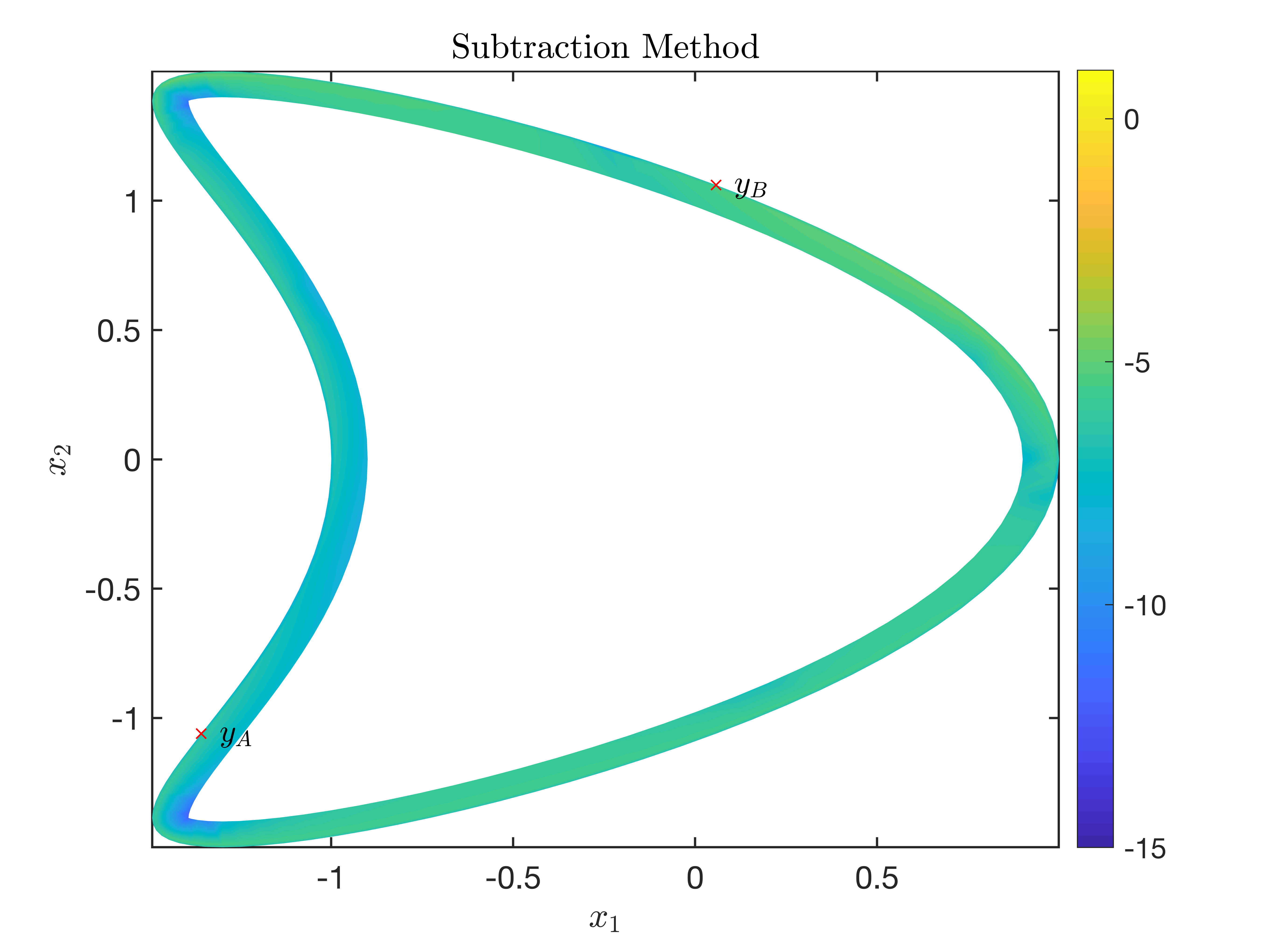
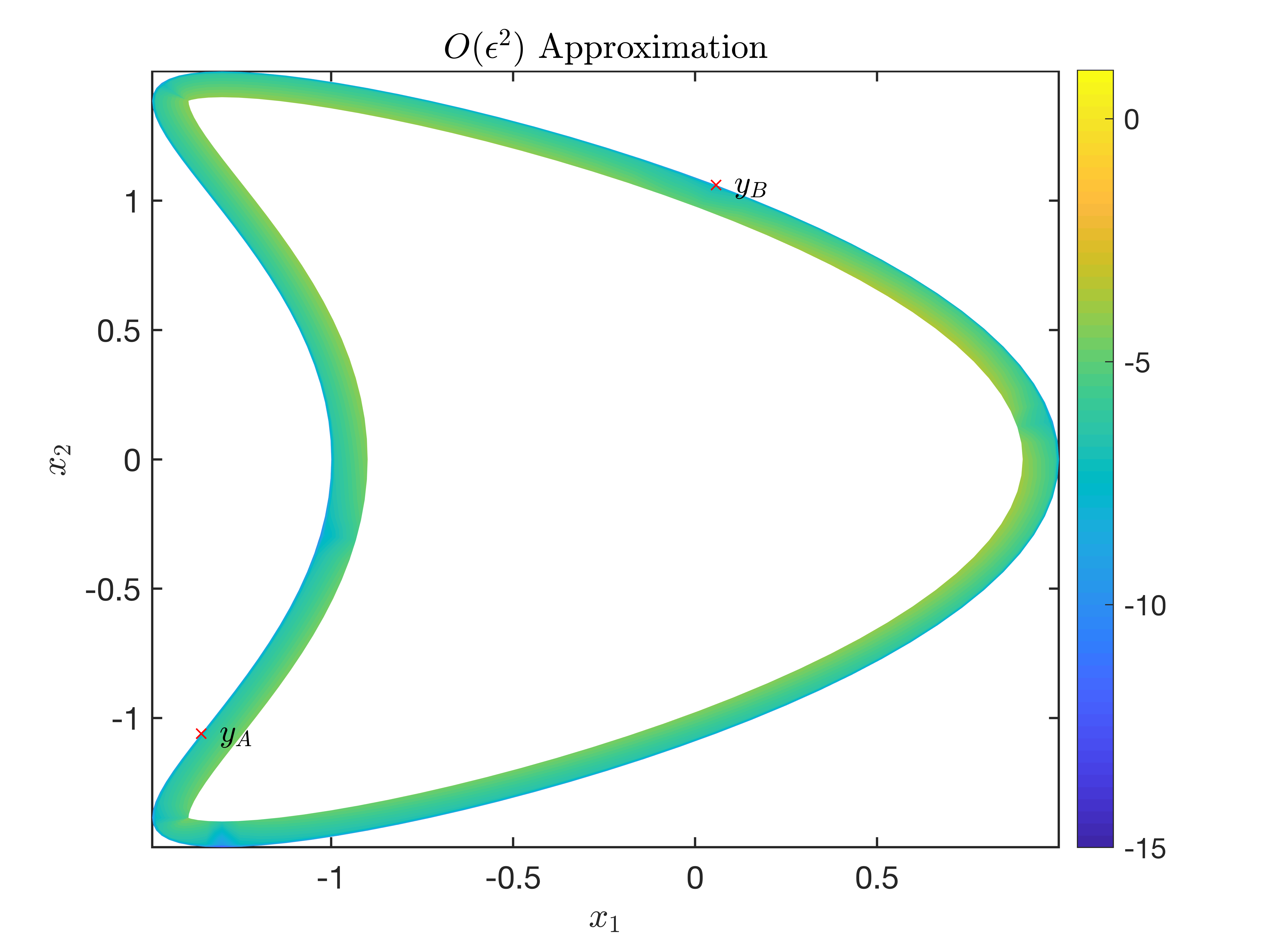
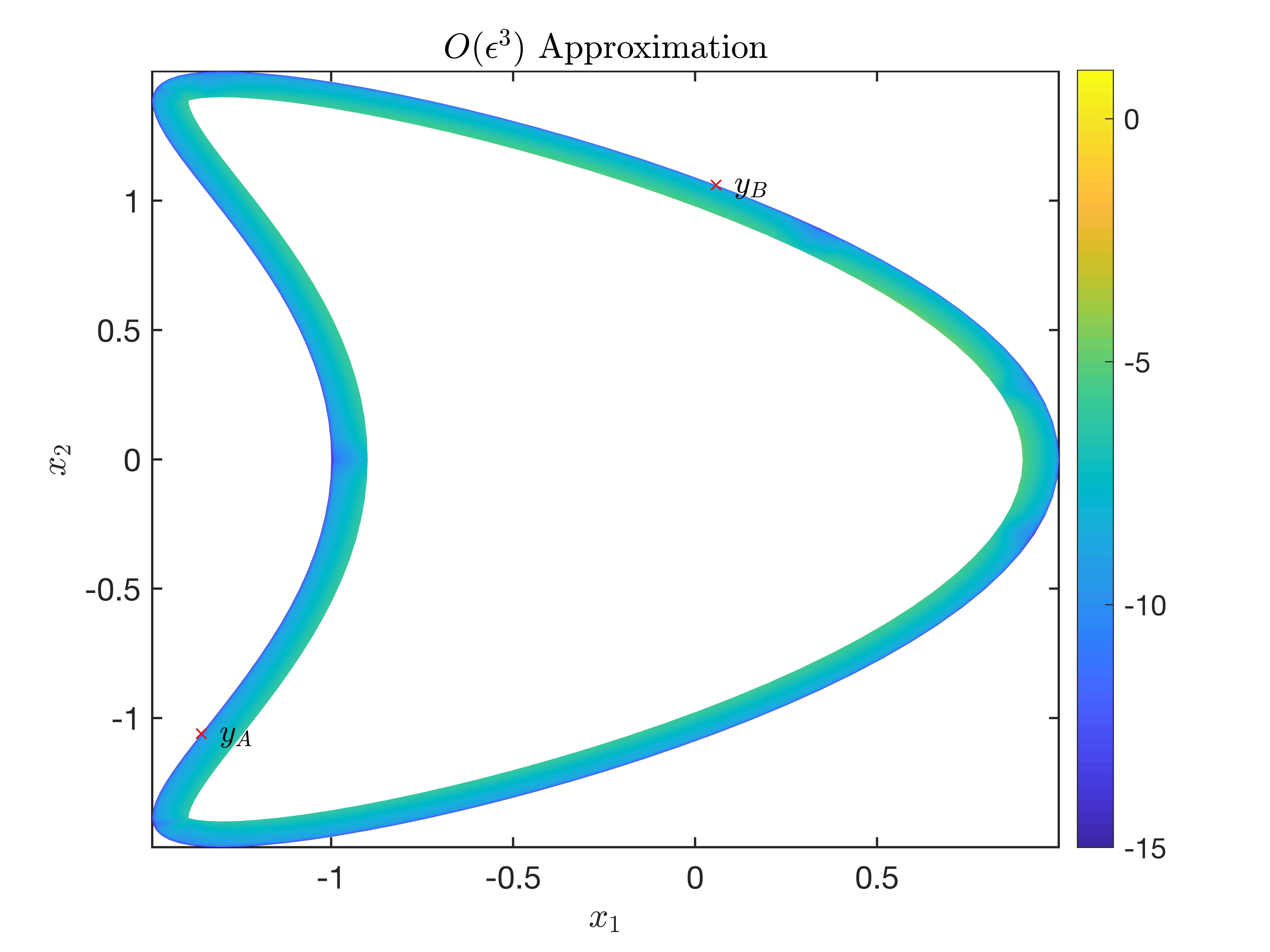
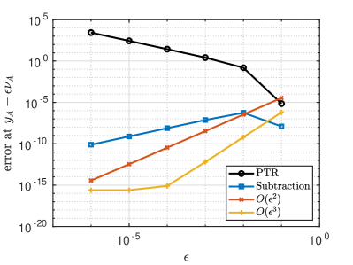
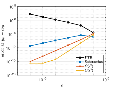
Figure 2: Plots of $\log_{10}$ of the error for the evaluation of the double-layer potential in the kite domain defined by (6.2) using four methods: the PTR method (upper left), the subtraction method (upper right), the $O(\varepsilon^{2})$ asymptotic approximation method (lower left), and the $O(\varepsilon^{3})$ asymptotic approximation method (lower right). In each of these plots, boundary points $y_{A}=(-1.3571,-1.0607)$ and $y_{B}=(0.0571,1.0607)$ are plotted as red $\times$’s.

Figure 3: Log-log plots of the errors made in computing the double-layer potential by the four methods shown in Fig. 3 at $y_{A}-\varepsilon\nu_{A}$ (left) and at $y_{B}-\varepsilon\nu_{B}$ (right) for $10^{-6}\leq\varepsilon\leq 10^{-1}$.

To compare the four methods more quantitatively, in Fig. 3 we plot the errors made by the four methods at $y_{A}-\varepsilon\nu_{A}$ (left) and $y_{B}-\varepsilon\nu_{B}$ (right) with $10^{-6}\leq\varepsilon\leq 10^{-1}$ where $\nu_{A}$ and $\nu_{B}$ are the unit outward normals at $y_{A}=(-1.3571,-1.0607)$, and $y_{B}=(0.0571,1.0607)$, respectively. The points $y_{A}$ and $y_{B}$ are shown in each plot of Fig. 3. From the results in Fig. 3 we observe that, the error when using the PTR method increases as $\varepsilon\to 0^{+}$, while the error in the other three methods decreases. The errors made by the asymptotic approximations are monotonically decreasing as $\varepsilon\to 0^{+}$. However, the error made by the subtraction method presents a different behavior: it reaches a maximum at $\varepsilon\approx 10^{-2}$ after which it decreases as $\varepsilon$ increases. For larger values of $\varepsilon$, the double-layer potential is no longer nearly singular, so the $N$-point PTR (and therefore methods 1 and 2) become more accurate. The error is at a maximum for the subtraction method when $\varepsilon=O(1/N)$, which is why we observe the maximum error occuring at $\varepsilon\approx 10^{-2}$. The results in Fig. 3 show a clear difference in the rate at which the errors vanish as $\varepsilon\to 0^{+}$ between the subtraction method and the asymptotic approximation methods. The $O(\varepsilon^{3})$ asymptotic approximation decays the fastest, followed by the $O(\varepsilon^{2})$ asymptotic approximation, and then the subtraction method. For $\varepsilon<10^{-4}$, the error incurred by the $O(\varepsilon^{3})$ asymptotic approximation levels out at machine precision. We estimate the rate at which the subtraction method and the asymptotic approximation methods decay with respect to $\varepsilon$ from the slope of the best fit line through the $\log-\log$ plot of the error versus $\varepsilon$ in Fig. 4. We compute the slope for each evaluation point $y(t_{j})-\varepsilon\tilde{\nu}(t_{j})$ where $t_{j}=-\pi+2(j-1)\pi/N$ for $j=1,\cdots,N$, and we vary $\varepsilon$. For the subtraction method, we consider $\varepsilon$ values such that $10^{-6}\leq\varepsilon\leq 10^{-2}$, and for the $O(\varepsilon^{2})$ and $O(\varepsilon^{3})$ asymptotic approximation methods, we consider the same range but only include values where the error is greater than $10^{-15}$. The results shown in Fig. 4 indicate that the subtraction method decays linearly with $\varepsilon$, and the rates of the asymptotic approximations are consistent with the theory presented in Section 3.

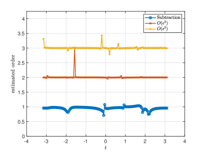
Figure 4: Estimated order of accuracy in computing the double-layer potential in the kite domain when using the subtraction method (blue $\circ$), the $O(\varepsilon^{2})$ asymptotic approximation method (red $\times$), and the $O(\varepsilon^{3})$ asymptotic approximation method (yellow $+$) for varying values of $t$.

For the second example of computing the double-layer potential in the star domain, Figures 6, 6, and 7 are analogous to Figures 3, 3, and 4 for the kite domain. The characteristics of the errors for this second domain are exactly the same as described for the kite domain.

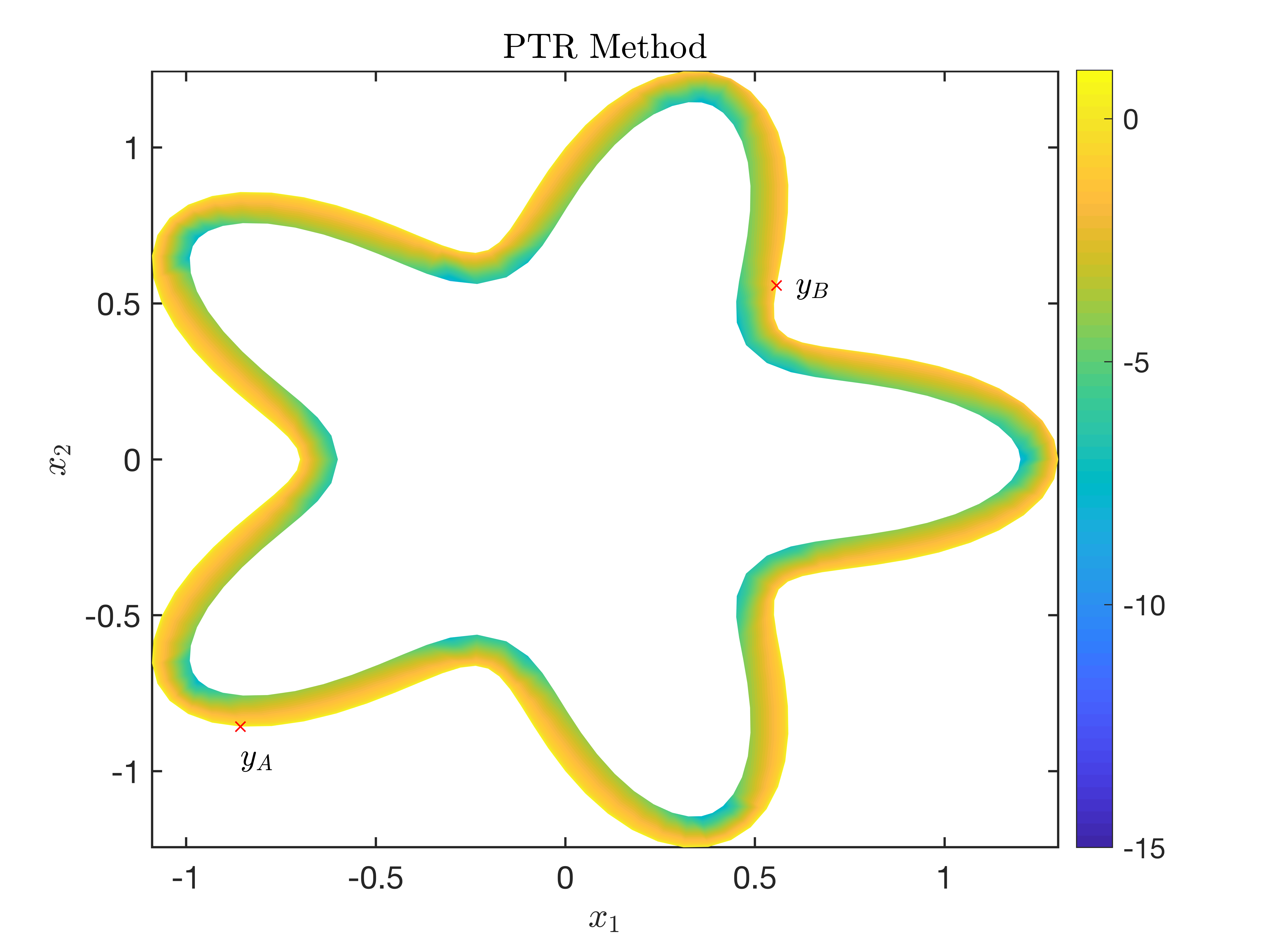
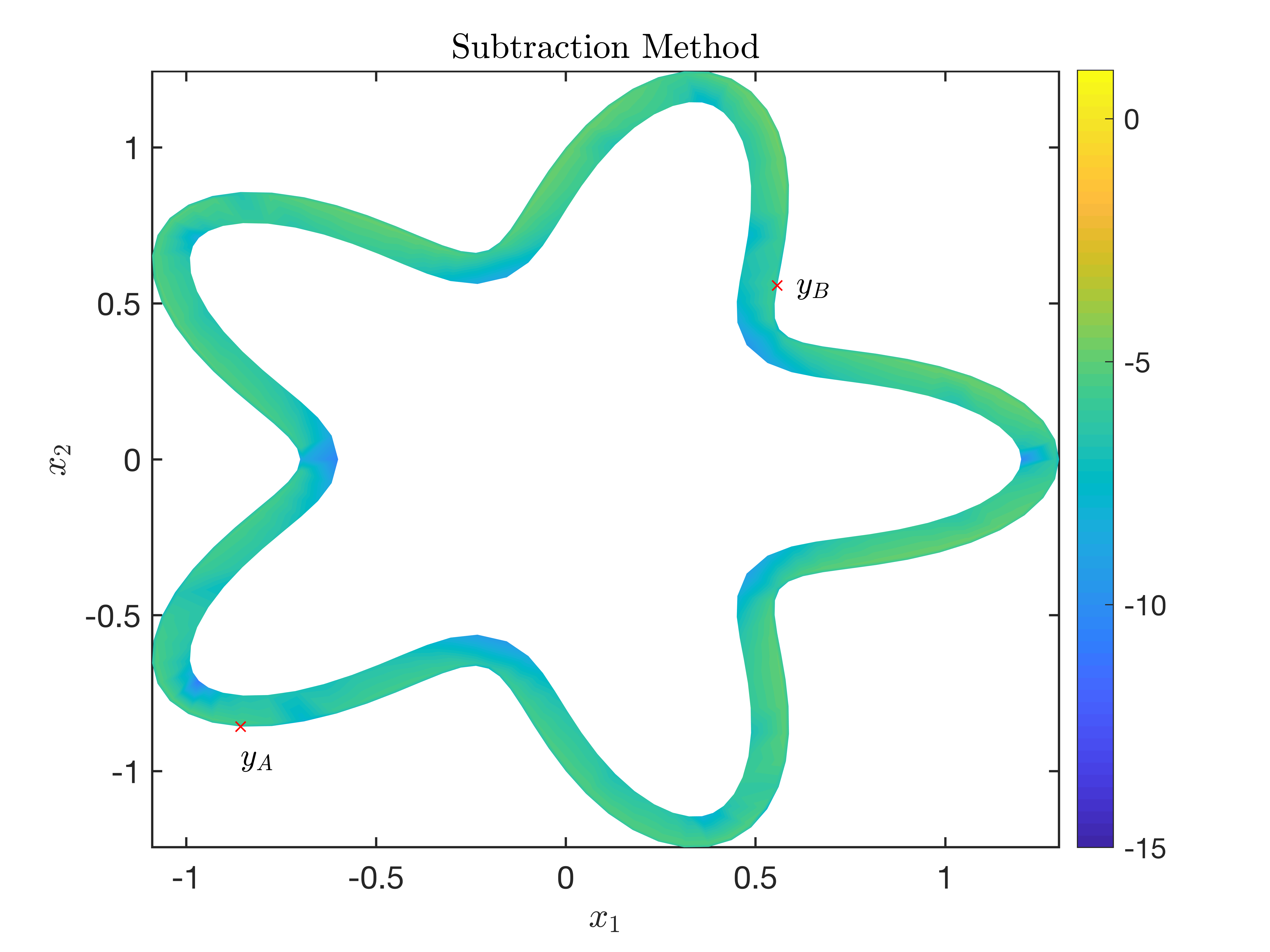
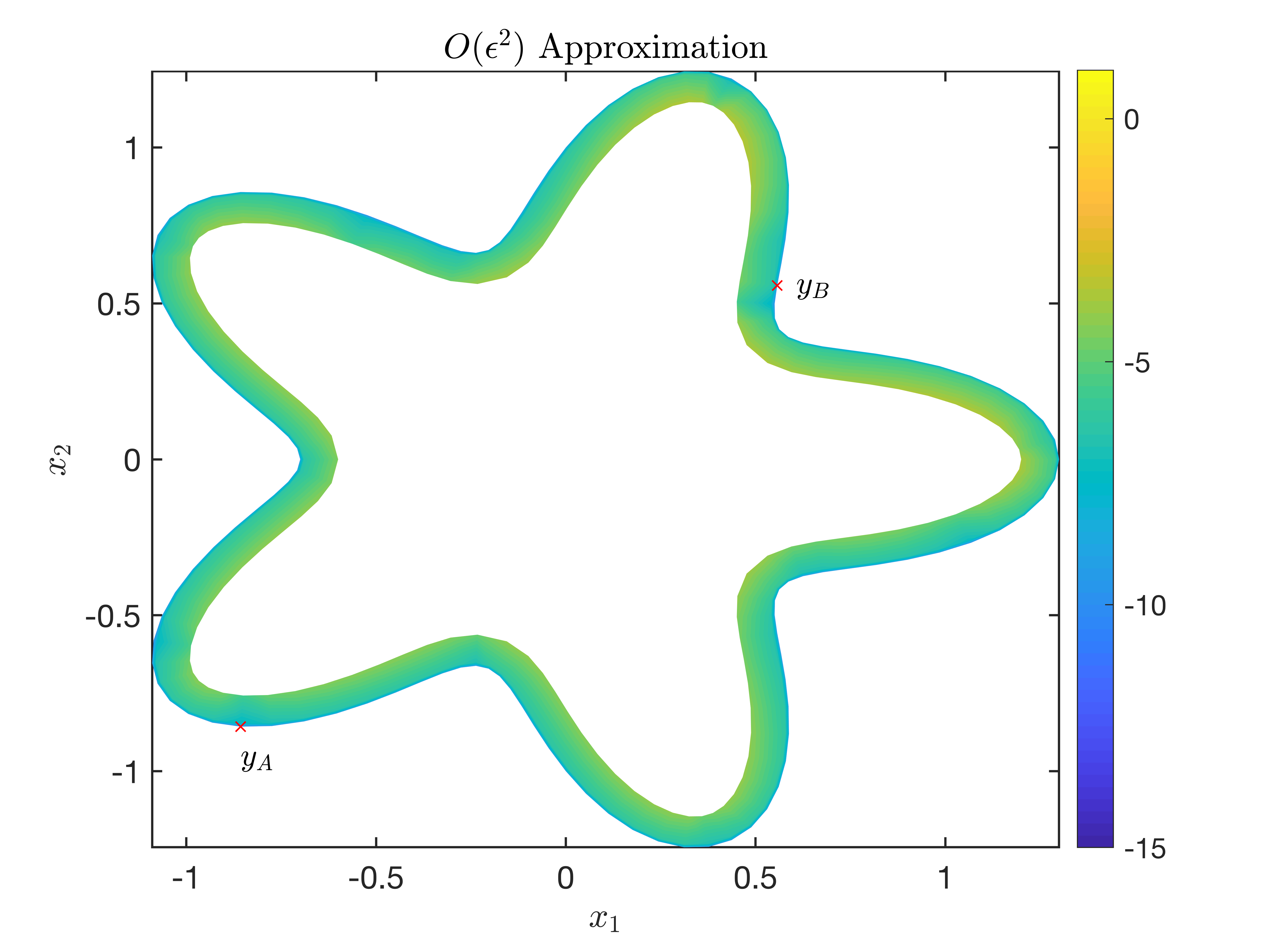
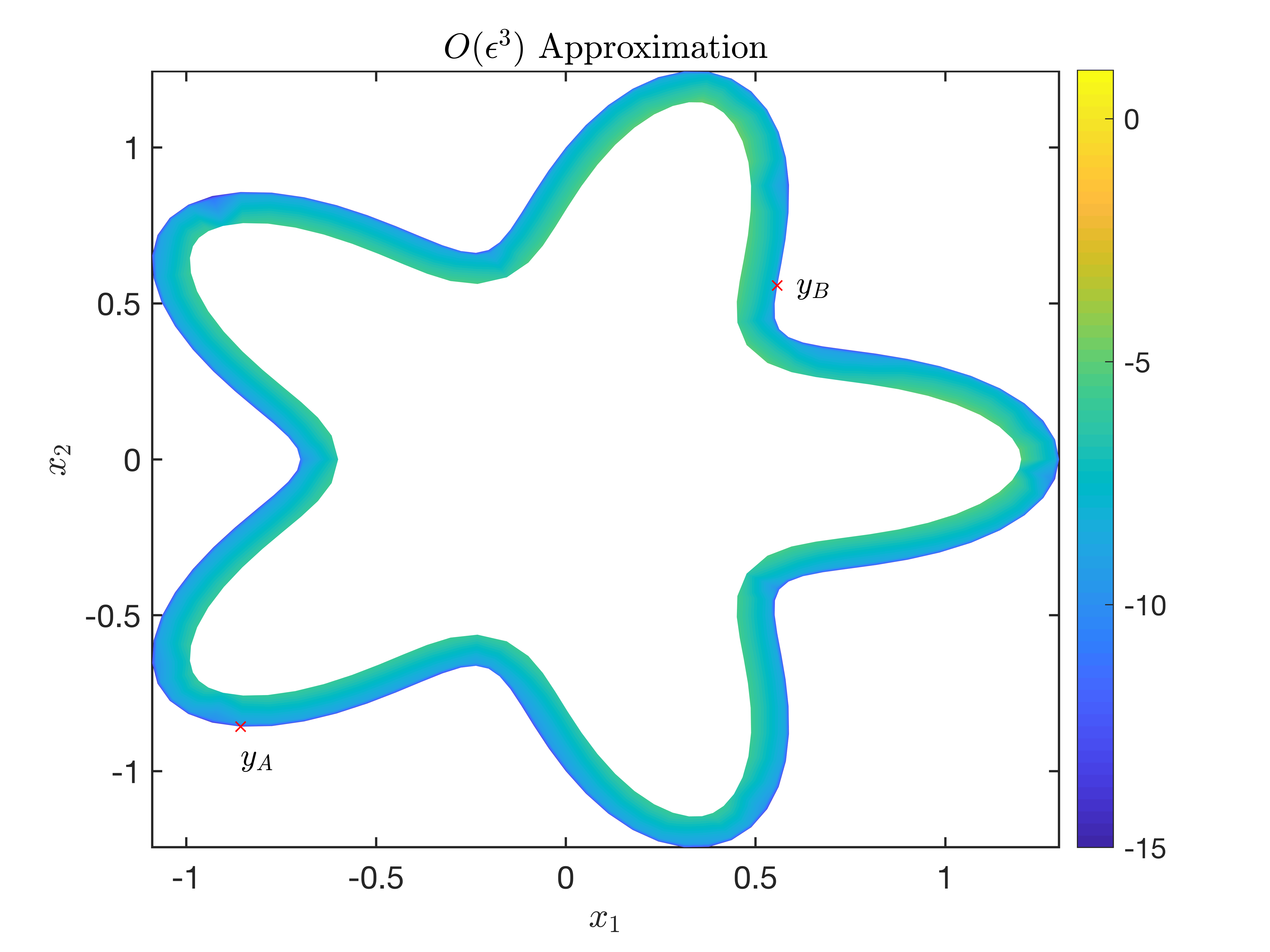
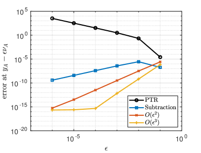
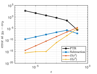
Figure 5: Plots of $\log_{10}$ of the error for the evaluation of the double-layer potential in the star domain defined by (6.3) using four methods: the PTR method (upper left), the subtraction method (upper right), the $O(\varepsilon^{2})$ asymptotic approximation method (lower left), and the $O(\varepsilon^{3})$ asymptotic approximation method (lower right). In each of these plots, boundary points $y_{A}=(-1.3571,-1.0607)$ and $y_{B}=(0.0571,1.0607)$ are plotted as red $\times$’s.

Figure 6: Log-log plots of the errors made in computing the double-layer potential by the four methods shown in Fig. 6 at $y_{A}-\varepsilon\nu_{A}$ (left) and at $y_{B}-\varepsilon\nu_{B}$ (right) for $10^{-6}\leq\varepsilon\leq 10^{-1}$.

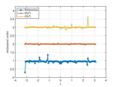
Figure 7: Estimated order of accuracy in computing the double-layer potential in the star domain when using the subtraction method (blue $\circ$), the $O(\varepsilon^{2})$ asymptotic approximation method (red $\times$), and the $O(\varepsilon^{3})$ asymptotic approximation method (yellow $*$) for varying values of $t$.

Summary of the results

In the case of two dimensional-problems, the subtraction method yields a method whose error decays linearly with the distance away from the boundary. The $O(\varepsilon^{2})$ and $O(\varepsilon^{3})$ asymptotic approximations methods are much more accurate for close evaluation points. Moreover, only relatively modest resolution is required for these asymptotic approximations to be effective. However, the error for these asymptotic approximations are monotonically increasing with the distance to the boundary, so they are not accurate for points further away from the boundary. The error estimates provided by the asymptotic theory provide guidance on where to apply these asymptotic approximations effectively. For all of these reasons, we find that the asymptotic approximations and corresponding numerical methods are quite useful for two-dimensional problems.

6.2 Three dimensions

Let $(x_{1},x_{2},x_{3})$ denote an ordered triple in a Cartesian coordinate system. To study the computation of the double-layer potential in three dimensions, we consider the harmonic function,

$$u(x_{1},x_{2},x_{3})=\frac{1}{\sqrt{(x_{1}-5)^{2}+(x_{2}-4)^{2}+(x_{3}-3)^{2}}}$$ (6.4)

in the domain whose boundary is given by

$$y(\theta,\varphi)=R(\theta)(\sin\theta\cos\varphi,2\sin\theta\sin\varphi,\cos\theta),\quad 0\leq\theta\leq\pi,\quad-\pi\leq\varphi\leq\pi,$$ (6.5)

with

$$R(\theta)=2-\frac{1}{1+100(1-\cos\theta)^{2}}.$$ (6.6)

This boundary surface is shown in Fig. 8 (left) along with its intersection with the vertical $x_{1}x_{3}$-plane (center) and the horizontal $x_{1}x_{2}$-plane (right).

We solve boundary integral equation (2.4) using the Galerkin method [4, 5, 6, 7]. The Galerkin method approximates the density according to

$$\tilde{\mu}(\theta,\varphi)\approx\tilde{\mu}^{N}(\theta,\varphi)=\sum_{n=0}^{N-1}\sum_{m=-n}^{n}\hat{\mu}_{nm}Y_{nm}(\theta,\varphi),$$ (6.7)

with $\{Y_{nm}\}$ denoting the orthonormal set of spherical harmonics. For these results, we have set $N=48$.

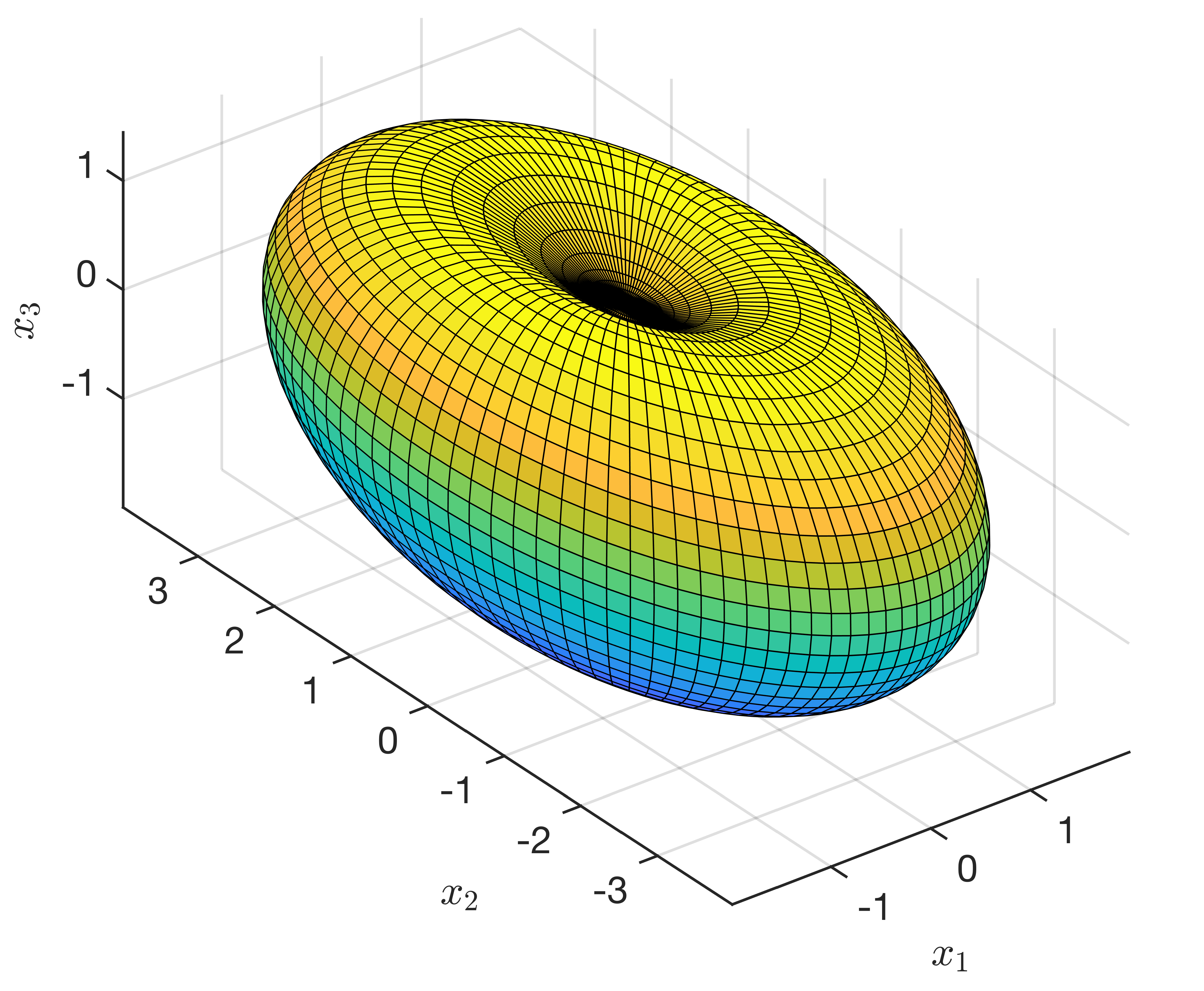
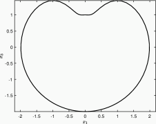
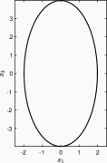
Figure 8: The boundary surface defined by (6.5)-(6.6) that is used to exemplify the evaluation of the double layer potential in three dimensions (left), and the intersections of this boundary with the $x_{1}x_{3}$-plane (center), and $x_{1}x_{2}$-plane (right).

We have computed the close evaluation of the double-layer potential at points $x=y^{\star}-\varepsilon\nu^{\star}$, using the following two different methods for comparison.

1. Numerical approximation – Compute the modified double-layer potential,

   $$u(y^{\star}-\varepsilon\nu^{\star})=-\mu(y^{\star})+\frac{1}{4\pi}\int_{B}\frac{\nu_{y}\cdot(y^{\star}-\varepsilon\nu^{\star}-y)}{|y^{\star}-\varepsilon\nu^{\star}-y|^{3}}\left[\mu(y)-\mu(y^{\star})\right]\mathrm{d}\sigma_{y},$$

   using the three-step numerical method given by Carvalho et al. [13]. For the first step, the modified double-layer potential is written as a spherical integral that has been rotated so that $y^{\star}$ is aligned with the north pole. For the second step, the $2N$-point PTR is used to compute the integral in the azimuthal angle. For the third step, the $N$-point Gauss-Legendre quadrature rule mapped to $[0,\pi]$ is used to compute the integral in the polar angle.

2. $O(\varepsilon^{2})$ Asymptotic approximation – Compute the asymptotic approximation given by (4.22) using the method given in (5.18) (with $N=48$).

The error of the numerical method has been shown to decay quadratically with $\varepsilon$ when $\varepsilon\ll 1/N$ [13]. This quadratic error decay occurs because, in the rotated coordinate system, the azimuthal integration acts as an averaging operation yielding a smooth function of the polar angle that is computed to high order using Gaussian quadrature. However, this asymptotic error estimate is valid only when the numerical approximation of the density is sufficiently resolved. If $N$ in (6.7) is not sufficiently large that $|\hat{\mu}_{nm}|$ for $n>N$ is negligibly small, then the truncation error associated with (6.7) may interrupt this quadratic error decay. For the domain here, with $N=48$, we find that the estimated truncation error for (6.7) is approximately $10^{-8}$. While this error is relatively small, it is not small enough to observe the error’s quadratic rate of decay. We would have to consider a much larger value of $N$ to observe that decay rate. However, computing the numerical solution of boundary integral equation (2.4) with $N>48$ becomes restrictively large. Hence, we evaluate below what the subtraction method and the $O(\varepsilon^{2})$ asymptotic approximation do in this limited resolution situation.

Error results for the computation of the double-layer potential in this domain for each of the two methods described above appear in Fig. 10. The top row shows the error on the slice of the domain through the vertical $x_{1}x_{3}$-plane for the numerical method (left) and the $O(\varepsilon^{2})$ asymptotic approximation method (right).The point $y_{A}=(1.7830,0,0.8390)$ is plotted as a red $\times$ symbol in both plots. The bottom row shows the errors of the same methods (left for the numerical method, right for the $O(\varepsilon^{2})$ asymptotic approximation) on the slice of the domain through the horizontal $x_{1}x_{2}$-plane. The point $y_{B}=(1.7439,1.19175,0)$ is plotted as a red $\times$ symbol in both plots.

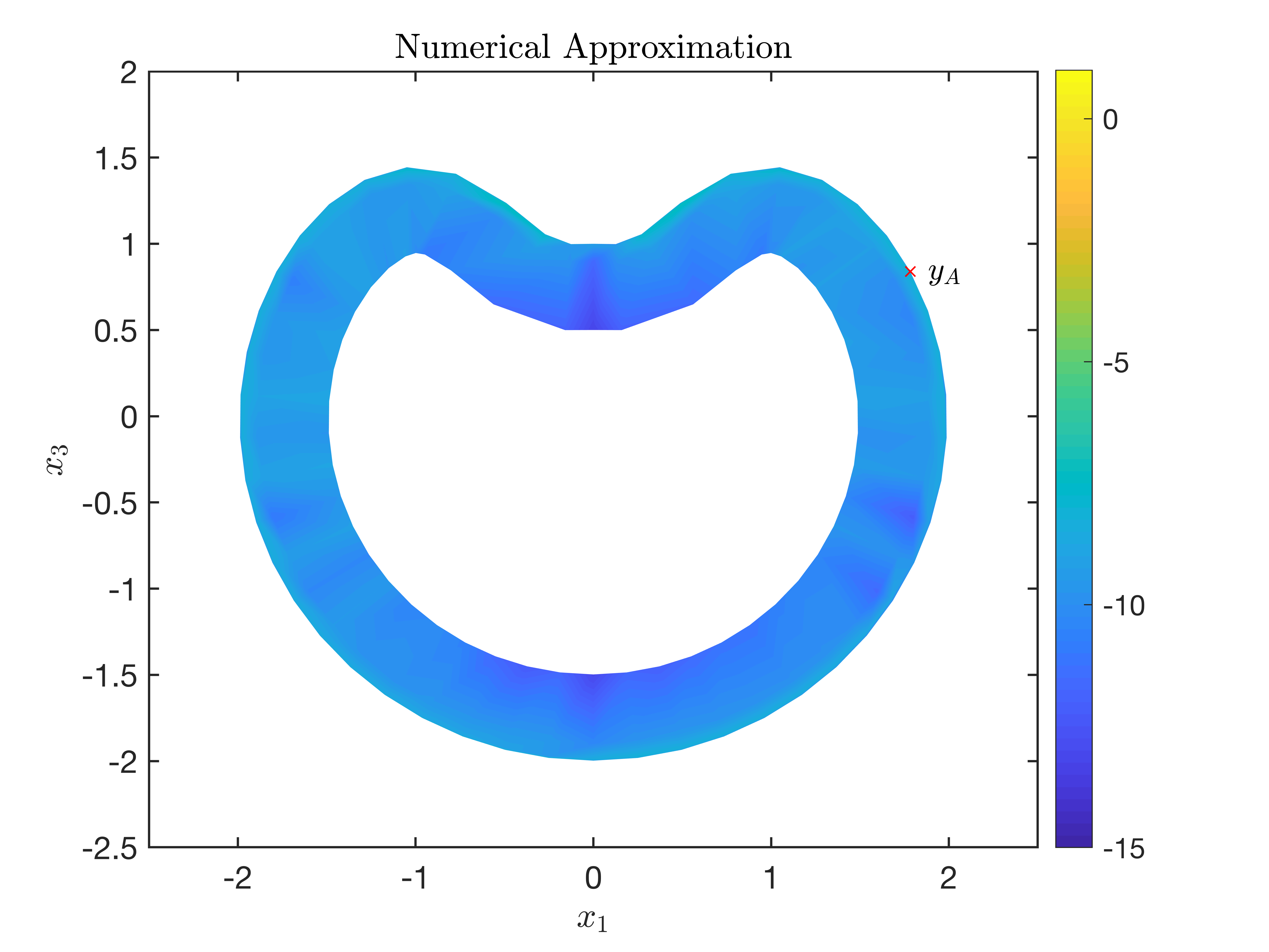
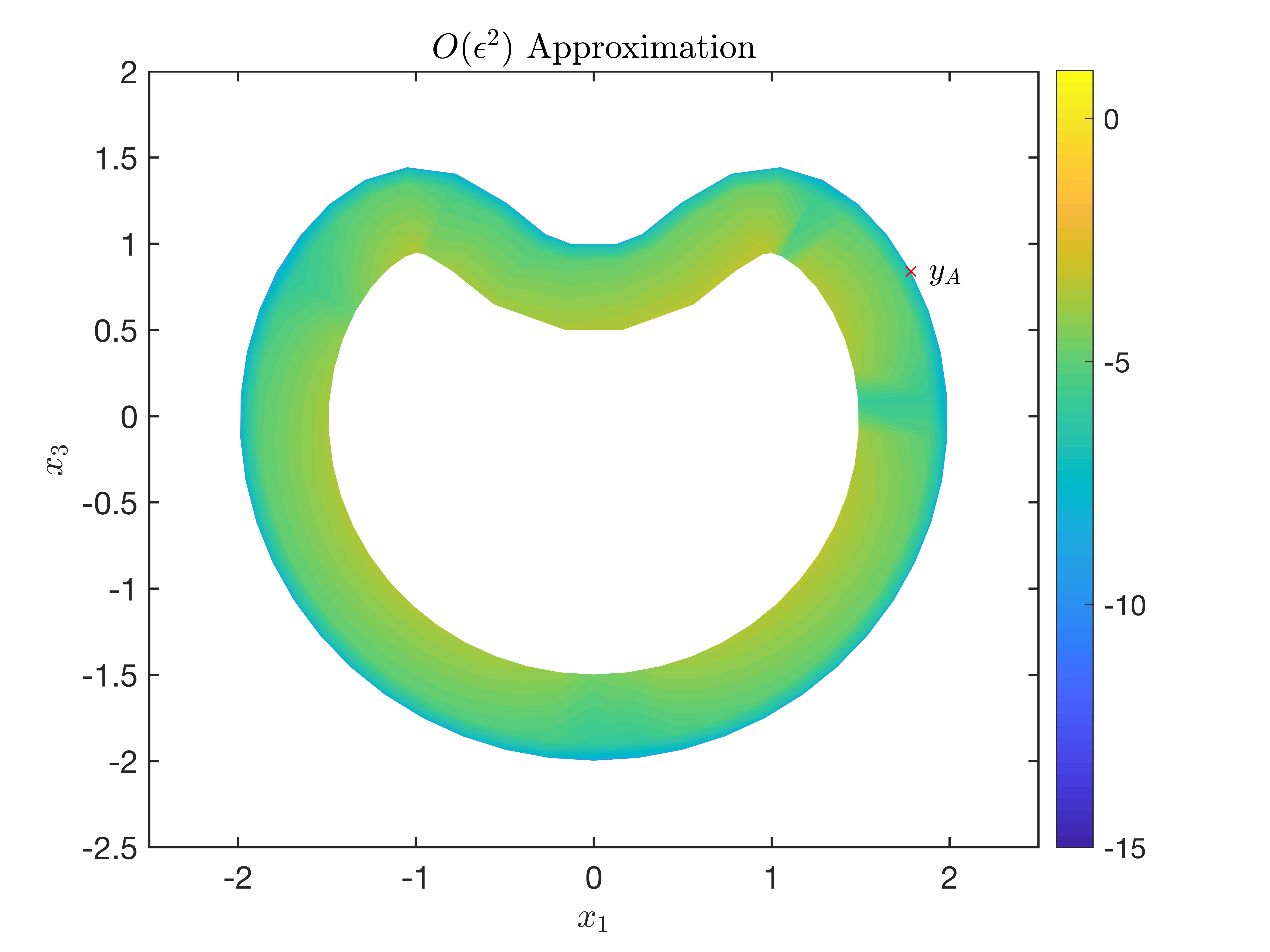
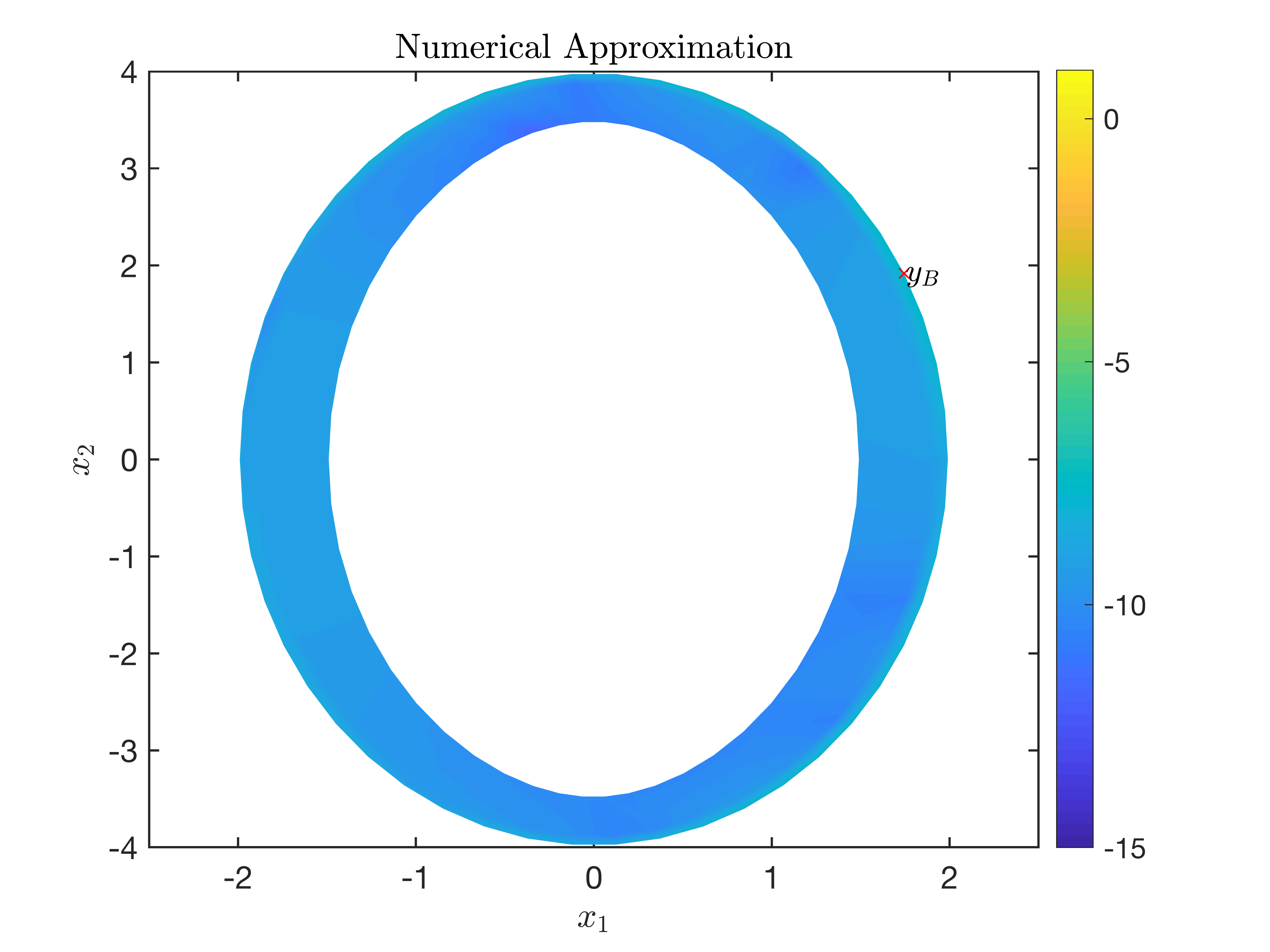
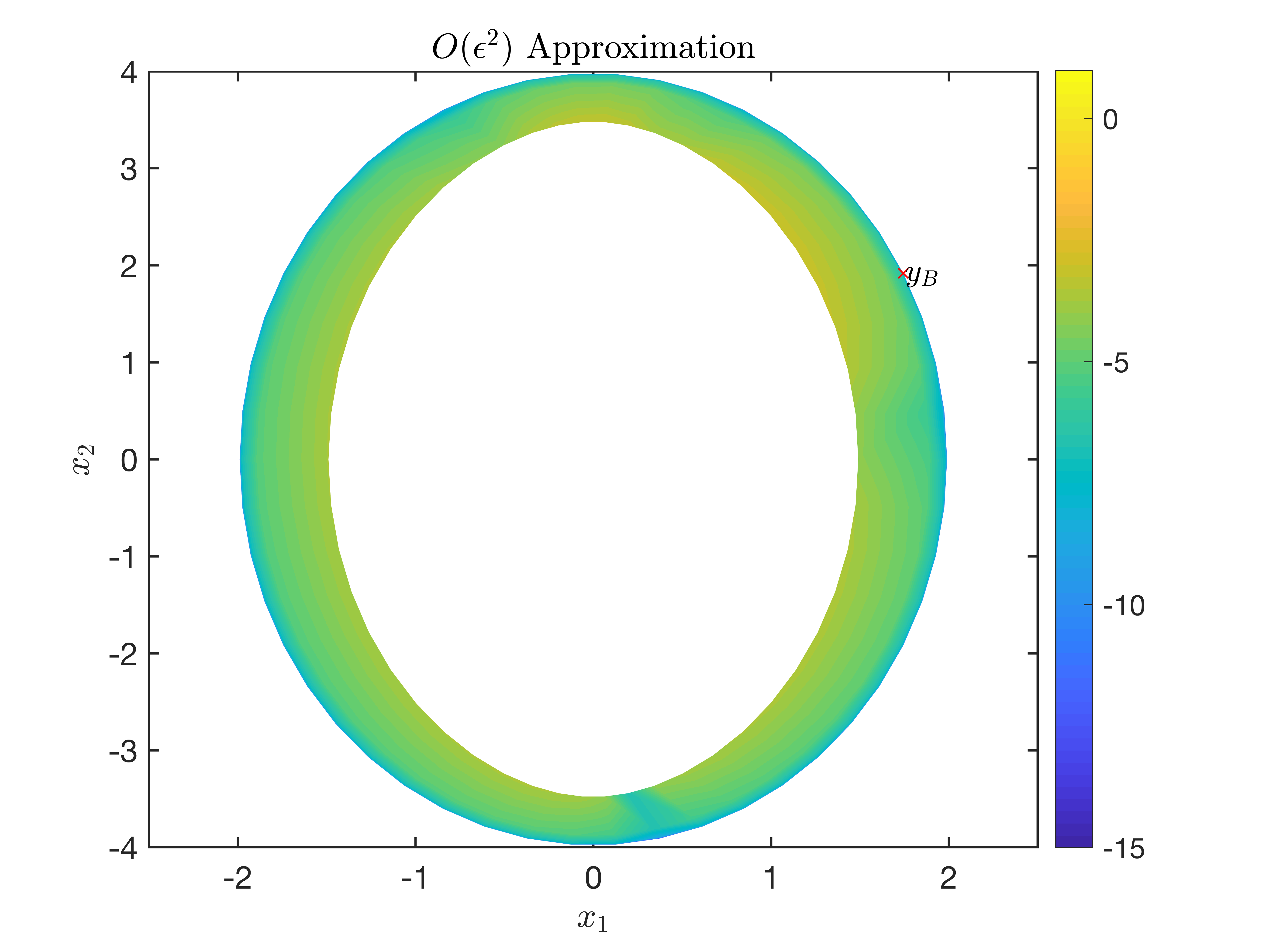
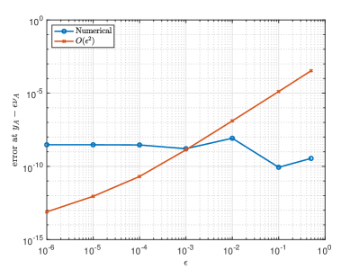
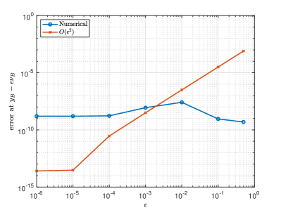
Figure 9: Plots of $\log_{10}$ of the error made in computing the double-layer potential by the numerical approximation (left column) and the $O(\varepsilon^{2})$ asymptotic approximation (right column) in the domain whose boundary is shown in Fig. 8. The top row of plots show the error on the $x_{1}x_{3}$-plane, and the bottom row of plots show the error on the $x_{1}x_{2}$-plane. In the top row of plots, the point $y_{A}=(1.7830,0,0.8390)$ is plotted as a red $\times$, and in the bottom row of plots, the point $y_{B}=(1.7439,1.19175,0)$ is plotted as a red $\times$.

Figure 10: Log-log plots of the errors made by the two methods shown in Fig. 10 at $y_{A}-\varepsilon\nu_{A}$ (left) and at $y_{B}-\varepsilon\nu_{B}$ (right) for $10^{-6}\leq\varepsilon\leq 0.5$.

In Fig. 10, we show the errors computed at $y_{A}-\varepsilon\nu_{A}$ (left) and $y_{B}-\varepsilon\nu_{B}$ (right) for varying $\varepsilon$, where $\nu_{A}$ and $\nu_{B}$ are the unit outward normals at $y_{A}$, and $y_{B}$, respectively. In contrast to the two-dimensional results, we find that the error for the numerical method is approximately $10^{-8}$ for all values of $\varepsilon$. This error is due to the truncation error made by the Galerkin method. Because the truncation error dominates at this resolution, we are not able to see its quadratic decay as $\varepsilon\to 0^{+}$. If a higher resolution computation was used to solve the boundary integral equation, the error of the numerical method would exhibit a similar behavior to that made by the subtraction method for the two-dimensional examples. In particular, the error would have a maximum at $\varepsilon=O(1/N)$ about which the error decays. We observe that the $O(\varepsilon^{2})$ asymptotic method decays monotonically with $\varepsilon$ even when $N=48$.

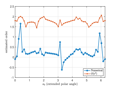
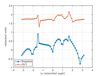
Figure 11: Estimated order of accuracy for the numerical approximation (blue $\circ$), and the $O(\varepsilon^{2})$ asymptotic approximation (red $\times$) on the $x_{1}x_{3}$-plane (left plot) and on the $x_{1}x_{2}$-plane (right plot). Results on the $x_{1}x_{3}$-plane are given in terms of the extended polar angle, $s_{0}\in[0,2\pi]$, which parameterizes the circle on the unit sphere lying on the $x_{1}x_{3}$-plane that starts and ends at the north pole. Results on the $x_{1}x_{2}$-plane are given in terms of the azimuthal angle, $t_{0}\in[0,2\pi]$.

We estimate the order of accuracy in Fig. 11. The results for the esimated order of accuracy over the points intersecting the vertical $x_{1}x_{3}$-plane are shown in the left plot of Fig. 11. For those results we determine the estimated order of accuracy by determining the best fit line through the $\log-\log$ plot of the error versus $\varepsilon$ for several values of the extended polar angle, $s_{0}\in[0,2\pi]$. This extended polar angle parameterizes the circle on the unit sphere lying on the $x_{1}x_{3}$-plane that starts and ends at the north pole. The results for the esimated order of accuracy over the points intersecting the horizontal $x_{1}x_{2}$-plane are shown in the right plot of Fig. 11. For those results we determine the estimated order of accuracy by determining the best fit line through the $\log-\log$ plot of the error versus $\varepsilon$ for several values of the azimuthal angle, $t_{0}\in[0,2\pi]$. Because of the resolution limitation in the Galerkin method, we are not able to see that the order of accuracy for the numerical method is two. In fact, the error is nearly uniform with respect to $\varepsilon$ because it is the truncation error of (6.7) that is dominating. Despite the resolution limitation in the Galerkin method, we find that the $O(\varepsilon^{2})$ asymptotic approximation has an order accuracy of nearly two.

Summary of the results

For three-dimensional problems, the subtraction method is more effective when computed in an appropriate rotated coordinate system than for two-dimensional problems. The subtraction method is more effective in three dimensions because in this rotated coordinate system, integration with respect to the azimuthal angle is a natural averaging operation that regularizes the integral thereby allowing for the use of a high-order quadrature rules for integration with respect to the polar angle. Provided that the density is sufficiently resolved, the subtraction method has been shown to decay quadratically with the distance away from the boundary [13]. The $O(\varepsilon^{2})$ asymptotic approximation also decays quadratically. However, it is not as sensitive to the accuracy of the density. For this reason, we find that the asymptotic approximation is still useful for three-dimensional problems, especially when the density is not highly resolved.

7 Extension to forward-peaked scattering in radiative transfer

The asymptotic approximations developed here for the close evaluation of the double-layer potential can be extended to other problems. In particular, there is an interesting connection between the close evaluation problem in potential theory and forward-peaked scattering in radiative transfer. We first establish this connection and then, we apply the asymptotic analysis used above to this problem.

Radiative transfer describes the multiple scattering of light [14, 20]. This theory has several applications for light propagation and scattering in geophysical media [32, 42], biological tissues [44], and computer graphics [21], among others. Let $\psi:S^{2}\times\mathbb{R}^{3}\times(0,T)\to\mathbb{R}^{+}\geq 0$ denote the specific intensity. The specific intensity gives the flow of power in direction $\Omega\in S^{2}$, at position $r\in\mathbb{R}^{3}$, at time $t\in[0,T]$. The radiative transfer equation,

$$c^{-1}\psi_{t}+\Omega\cdot\nabla\psi+\mu_{a}\psi-\mu_{s}L\psi=Q,$$ (7.1)

governs $\psi$ in a medium that absorbs, scatters, and emits light. Here, $c$ denotes the speed of light in the background medium, $\mu_{a}\geq 0$, $\mu_{s}\geq 0$ denote absorption and scattering coefficients, respectively, and $Q$ denotes a source. The scattering operator, $L$, is defined by

$$L\psi(\Omega,r,t)=\displaystyle\frac{1}{4\pi}\int_{S^{2}}p(\Omega\cdot\Omega^{\prime})\left[\psi(\Omega^{\prime},r,t)-\psi(\Omega,r,t)\right]\mathrm{d}\sigma_{\Omega^{\prime}},$$ (7.2)

where $p$ denotes the scattering phase function which gives the fraction of light incident in direction $\Omega^{\prime}$ that is scattered in direction $\Omega$.

In forward-peaked scattering media, $p$ is sharply peaked about $\Omega=\Omega^{\prime}$ so that most of the scattering occurs in a small angular cone about the incident direction. This problem is important for several applications, especially light propagation in biological tissues [24]. Mathematically, forward-peaked scattering corresponds to the case in which (7.2) is a nearly singular integral.

There have been several studies on the asymptotic behavior of (7.1) with forward-peaked scattering leading to the Fokker-Planck approximation [35] and its generalizations [37, 29]. Solving the radiative transfer equation (7.1) with these approximate scattering operators has led to useful physical insight [25, 26, 16]. However, for most scattering models used for applications, the Fokker-Planck approximation is inaccurate. The error made by the Fokker-Planck approximation is due to neglecting the tail away from the sharply peaked behavior of the kernel $p$, corresponding to large-angle scattering. That tail typically decays too slowly to make a local approximation appropriate. In fact, it has been shown that for several specific scattering kernels, the leading order behavior is nonlocal and given by a pseudo-differential operator [36, 28].

We study forward-peaked scattering using the same asymptotic analysis used to study the close evaluation of layer potentials discussed above. For this study, we consider the specific choice of the Henyey-Greenstein scattering phase function [19],

$$p_{\text{HG}}(\Omega\cdot\Omega^{\prime})=\frac{1-g^{2}}{(1+g^{2}-2g\Omega\cdot\Omega^{\prime})^{3/2}},\quad-1\leq g\leq 1,$$ (7.3)

as the kernel. The Henyey-Greenstein scattering phase function is extensively used in applications since it provides a simple model with enough sophistication to study multiple scattering of light. The anisotropy factor, $g$, is the mean cosine of the scattering angle. It sets the amount of scattering that is forward peaked. When $g=0$, scattering is istropic, and when $g=\pm 1$, scattering is restricted to only the forward/backward direction. Forward-peaked scattering corresponds to the asymptotic limit as $g\to 1$.

Henyey-Greenstein scattering is directly related to Poisson’s formula for the unit sphere,

$$u(x)=\frac{1}{4\pi}\int_{S^{2}}\frac{1-|x|^{2}}{|x-y|^{3}}f(y)\mathrm{d}\sigma_{y},\quad|x|<1,$$ (7.4)

which gives the solution of the boundary value problem for Laplace’s equation:

$$\varDelta u=0\quad\text{in $|x|<1$},$$ (7.5a)

$$u=f\quad\text{on $|x|=1$}.$$ (7.5b)

For the close evaluation point $x=(1-\varepsilon)y^{\star}$ with $|y^{\star}|=1$ and $0<\varepsilon\ll 1$, we find that

$$u((1-\varepsilon)y^{\star})=\frac{1}{4\pi}\int_{S^{2}}\frac{1-(1-\varepsilon)^{2}}{\left[1+(1-\varepsilon)^{2}-2(1-\varepsilon)y^{\star}\cdot y\right]^{3/2}}f(y)\mathrm{d}\sigma_{y}.$$ (7.6)

Notice that the kernel in (7.6) is the same as (7.3) with $g=1-\varepsilon$. Consequently, the asymptotic limit of forward-peaked Henyey-Greenstein scattering is closely related to the close evaluation of Poisson’s formula for the unit sphere.

To evaluate $L$ given in (7.2) using (7.3) as the scattering phase function, we use a spherical coordinate system with $\Omega$ defining its north pole. In this coordinate system, $\theta$ denotes the polar angle and $\phi$ denotes the azimuthal angle. For that case, we have

$$L\psi(\Omega)=\frac{1}{2}\int_{0}^{\pi}p_{\text{HG}}(\cos\theta;\varepsilon)\tilde{\psi}(\theta)\sin\theta\mathrm{d}\theta$$ (7.7)

with $\Omega\cdot\Omega^{\prime}=\cos\theta$, $g=1-\varepsilon$,

$$p_{\text{HG}}(\cos\theta;\varepsilon)=\frac{1-(1-\varepsilon)^{2}}{[1+(1-\varepsilon)^{2}-2(1-\varepsilon)\cos\theta]^{3/2}},$$ (7.8)

and

$$\tilde{\psi}(\theta)=\frac{1}{2\pi}\int_{-\pi}^{\pi}\left[\psi(\theta,\varphi)-\psi(0,\cdot)\right]\mathrm{d}\varphi.$$ (7.9)

Due to the regularity of the solution at the north pole, we have $\psi(\theta,\varphi+\pi)=\psi(-\theta,\varphi)$. As a result, we write

$$\tilde{\psi}(\theta)=\frac{1}{2\pi}\int_{0}^{\pi}\left[\psi(\theta,\varphi)+\psi(-\theta,\varphi)-2\psi(0,\cdot)\right]\mathrm{d}\varphi.$$ (7.10)

Note here $\psi(0,\cdot)=\psi(\Omega)$. To study forward-peaked scattering we study the asymptotic limit corresponding to $\varepsilon\to 0^{+}$.

We let

$$L\psi(\Omega)=L^{\text{in}}\psi(\Omega)+L^{\text{out}}\psi(\Omega),$$ (7.11)

where

$$L^{\text{in}}\psi(\Omega)=\frac{1}{2}\int_{0}^{\delta}p_{\text{HG}}(\cos\theta;\varepsilon)\tilde{\psi}(\theta)\sin\theta\mathrm{d}\theta,$$ (7.12)

is the inner expansion, and

$$L^{\text{out}}\psi(\Omega)=\frac{1}{2}\int_{\delta}^{\pi}p_{\text{HG}}(\cos\theta;\varepsilon)\tilde{\psi}(\theta)\sin\theta\mathrm{d}\theta,$$ (7.13)

is the outer expansion. Just as we have done for the double-layer potential, we consider the asymptotic limit in which $0<\varepsilon\ll\delta\ll 1$. Details of the calculations below can be found in a developed Mathematica notebook available on GitHub [23].

To find the leading-order behavior for $L^{\text{in}}$, we substitute (7.8) into (7.12) and make the substitution $\theta=\varepsilon\Theta$,

$$\begin{split}L^{\text{in}}\psi(\Omega)&=\int_{0}^{\delta/\varepsilon}\frac{1}{2}\frac{1-(1-\varepsilon)^{2}}{[1+(1-\varepsilon)^{2}-2(1-\varepsilon)\cos\varepsilon\Theta]^{3/2}}\tilde{\psi}(\varepsilon\Theta)\sin\varepsilon\Theta\varepsilon\mathrm{d}\Theta\\ &=\int_{0}^{\delta/\varepsilon}\left[\frac{\Theta}{(1+\Theta^{2})^{3/2}}-\frac{\varepsilon}{2}\frac{\Theta-2\Theta^{3}}{(1+\Theta^{2})^{5/2}}+O(\varepsilon^{2})\right]\tilde{\psi}(\varepsilon\Theta)\mathrm{d}\Theta.\end{split}$$ (7.14)

Next, we compute the expansion

$$\begin{split}\tilde{\psi}(\varepsilon\Theta)&=\frac{1}{2\pi}\int_{0}^{\pi}\left[\psi(\varepsilon\Theta,\varphi)+\psi(-\varepsilon\Theta,\varphi)-2\psi(0,\cdot)\right]\mathrm{d}\varphi\\ &=\frac{\varepsilon^{2}\Theta^{2}}{2\pi}\int_{0}^{\pi}\psi_{\theta\theta}(0,\cdot)\mathrm{d}\varphi+O(\varepsilon^{4}).\end{split}$$ (7.15)

Substituting (4.11) (see Appendix B) into this result, we find that

$$\tilde{\psi}(\varepsilon\Theta)=\frac{\varepsilon^{2}\Theta^{2}}{2\pi}\int_{0}^{\pi}\psi_{\theta\theta}(0,\cdot)\mathrm{d}\varphi+O(\varepsilon^{4})=\frac{\varepsilon^{2}\Theta^{2}}{4}\varDelta_{S^{2}}\psi(\Omega)+O(\varepsilon^{4}),$$ (7.16)

Substituting (7.16) into (7.14), we determine by integrating and then expanding about $\varepsilon=0$ that

$$\begin{split}L^{\text{in}}\psi(\Omega)&=\varDelta_{S^{2}}\psi(\Omega)\int_{0}^{\delta/\varepsilon}\left[\frac{\varepsilon^{2}\Theta^{3}}{4(1+\Theta^{2})^{3/2}}-\frac{\varepsilon^{3}}{8}\frac{\Theta^{3}-2\Theta^{5}}{(1+\Theta^{2})^{5/2}}+O(\varepsilon^{4})\right]\mathrm{d}\Theta,\\ &=\left[\frac{\varepsilon\delta}{4}-\frac{\varepsilon^{2}}{2}+\frac{\varepsilon^{2}\delta}{4}\right]\varDelta_{S^{2}}\psi(\Omega)+O(\varepsilon^{3}).\end{split}$$ (7.17)

To compute the outer expansion, we expand (7.8) about $\varepsilon=0$ then substitute the result into (7.13), and obtain

$$L^{\text{out}}\psi(\Omega)=\int_{\delta}^{\pi}\frac{\varepsilon+\varepsilon^{2}}{2\sqrt{2}(1-\cos\theta)^{3/2}}\tilde{\psi}(\theta)\sin\theta\mathrm{d}\theta+O(\varepsilon^{3}).$$ (7.18)

To remove $\delta$ from the lower limit of integration, we write

$$L^{\text{out}}\psi(\Omega)=\int_{0}^{\pi}\frac{\varepsilon+\varepsilon^{2}}{2\sqrt{2}(1-\cos\theta)^{3/2}}\tilde{\psi}(\theta)\sin\theta\mathrm{d}\theta-\int_{0}^{\delta}\frac{\varepsilon+\varepsilon^{2}}{2\sqrt{2}(1-\cos\theta)^{3/2}}\tilde{\psi}(\theta)\sin\theta\mathrm{d}\theta+O(\varepsilon^{3}).$$ (7.19)

For the second term in (7.19), we substitute $\theta=\varepsilon\Theta$ and find that

$$\begin{split}\int_{0}^{\delta/\varepsilon}\frac{\varepsilon+\varepsilon^{2}}{2\sqrt{2}(1-\cos\varepsilon\Theta)^{3/2}}&\tilde{\psi}(\varepsilon\Theta)\sin\varepsilon\Theta\varepsilon\mathrm{d}\Theta\\ &=\int_{0}^{\delta/\varepsilon}\left[\frac{1+\varepsilon}{\Theta^{2}}+O(\varepsilon^{2})\right]\tilde{\psi}(\varepsilon\Theta)\mathrm{d}\Theta\\ &=\varDelta_{S^{2}}\psi(\Omega)\int_{0}^{\delta/\varepsilon}\left[\frac{\varepsilon^{2}+\varepsilon^{3}}{4}+O(\varepsilon^{4})\right]\mathrm{d}\Theta\\ &=\left[\frac{\varepsilon\delta}{4}+\frac{\varepsilon^{2}\delta}{4}\right]\varDelta_{S^{2}}\psi(\Omega)+O(\varepsilon^{3}),\end{split}$$ (7.20)

where we have made use of (7.16) Thus, the leading-order asymptotic behavior for $L^{\text{out}}\psi(\Omega)$ is given by

$$L^{\text{out}}\psi(\Omega)=\frac{\varepsilon+\varepsilon^{2}}{2\sqrt{2}}\int_{0}^{\pi}\frac{\tilde{\psi}(\theta)}{(1-\cos\theta)^{3/2}}\sin\theta\mathrm{d}\theta-\left[\frac{\varepsilon\delta}{4}+\frac{\varepsilon^{2}\delta}{4}\right]\varDelta_{S^{2}}\psi(\Omega)+O(\varepsilon^{3}).$$ (7.21)

By summing (7.17) and (7.21), and substituting (7.10), we find that

$$L\psi(\Omega)=\left(\varepsilon+\varepsilon^{2}\right)L_{3/2}\psi(\Omega)-\frac{\varepsilon^{2}}{2}\varDelta_{S^{2}}\psi(\Omega)+O(\varepsilon^{3}).$$ (7.22)

where

$$L_{3/2}\psi(\Omega)=\frac{1}{4\sqrt{2}\pi}\int_{0}^{\pi}\int_{0}^{\pi}\frac{\psi(\theta,\varphi)+\psi(-\theta,\varphi)-2\psi(0,\cdot)}{(1-\cos\theta)^{3/2}}\sin\theta\mathrm{d}\theta\mathrm{d}\varphi.$$ (7.23)

The integral in (7.23) appears to be singular, but since

$$\frac{1}{4\sqrt{2}\pi}\int_{0}^{\pi}\frac{\psi(\theta,\varphi)+\psi(-\theta,\varphi)-2\psi(0,\cdot)}{(1-\cos\theta)^{3/2}}\sin\theta\mathrm{d}\varphi=\frac{1}{4}\varDelta_{S^{2}}\psi(\Omega)+O(\theta^{2}),$$ (7.24)

$L_{3/2}\psi(\Omega)$ is well defined.

The leading-order asymptotic behavior of $L$ given in (7.22) is equivalent to a result by Larsen [28, Eq. 31] who derived an asymptotic approximation for $L$ using a spectral analysis. In contrast to that asymptotic approximation, the asymptotic analysis given above directly addresses the balance between the forward peak given by the inner expansion, and the long tail given by the outer expansion of the scattering operator with the Henyey-Greenstein scattering kernel.

8 Conclusion

We have computed the leading-order asymptotic behavior for the close evaluation of the double-layer potential in two and three dimensions. By developing numerical methods to evaluate these asymptotic approximations, we obtain effective methods for computing double-layer potentials at close evaluation points. Our numerical examples demonstrate the effectiveness of these asymptotic approximations and corresponding numerical methods.

The key to this asymptotic analysis is the insight it provides. The leading-order asymptotic behavior of the close evaluation of the double-layer potential is given by its local Dirichlet data plus a correction that is nonlocal. It is this nonlocal term that makes the close evaluation problem challenging to address using only numerical methods. It is consistent with the fact that solutions of boundary value problems for elliptic partial differential equations have a global dependence on their boundary data. By explicitly computing this correction using asymptotic analysis, we have been able to develop an effective numerical method for it. Moreover, the asymptotic error estimates provide guidance on where to apply these approximations, namely, for evaluation points closer to the boundary than the boundary mesh spacing. The result of this work is an accurate and efficient method for computing the close evaluation of the double-layer potential.

The asymptotic approximation method can be extended to other layer potentials and other boundary value problems. In this paper, we show how these methods discover valuable insight for forward-peaked scattering in radiative transfer theory. Future work will entail of extending these methods to applications of Stokes flow and plasmonics.

Appendix A Rotations on the sphere

We give the explicit rotation formulas over the sphere used in the numerical method for the asymptotic approximation in three dimensions. Consider $y,y^{\star}\in S^{2}$. We introduce the parameters $\theta\in[0,\pi]$ and $\varphi\in[-\pi,\pi]$ and write

$$y=y(\theta,\varphi)=\sin\theta\cos\varphi\,\hat{\i}+\sin\theta\sin\varphi\,\hat{\j}+\cos\theta\,\hat{{\rm k}}.$$ (A.1)

The parameter values, $\theta^{\star}$ and $\varphi^{\star}$, are set such that that $y^{\star}=y(\theta^{\star},\varphi^{\star})$.

We would like to work in the rotated, $\rm uvw$-coordinate system in which

$$\hat{{\rm u}} =\cos\theta^{\star}\cos\varphi^{\star}\,\hat{\i}+\cos\theta^{\star}\sin\varphi^{\star}\,\hat{\j}-\sin\theta^{\star}\,\hat{{\rm k}},$$ (A.2)

$$\hat{{\rm v}} =-\sin\varphi^{\star}\,\hat{\i}+\cos\varphi^{\star}\,\hat{\j},$$

$$\hat{{\rm w}} =\sin\theta^{\star}\cos\varphi^{\star}\,\hat{\i}+\sin\theta^{\star}\sin\varphi^{\star}\,\hat{\j}+\cos\theta^{\star}\,\hat{{\rm k}}.$$

Notice that $\hat{\rm w}=y^{\star}$. For this rotated coordinate system, we introduce the parameters $s\in[0,\pi]$ and $t\in[-\pi,\pi]$ such that

$$y=y(s,t)=\sin s\cos t\,\hat{{\rm u}}+\sin s\sin t\,\hat{{\rm v}}+\cos s\,\hat{{\rm w}}.$$ (A.3)

It follows that $y^{\star}=y(0,\cdot)$. By equating (A.1) and (A.3) and substituting (A.2) into that result, we obtain

$$\begin{bmatrix}\sin\theta\cos\varphi\\ \sin\theta\sin\varphi\\ \cos\theta\end{bmatrix}=\begin{bmatrix}\cos\theta^{\star}\cos\varphi^{\star}&-\sin\varphi^{\star}&\sin\theta^{\star}\cos\varphi^{\star}\\ \cos\theta^{\star}\sin\varphi^{\star}&\cos\varphi^{\star}&\sin\theta^{\star}\sin\varphi^{\star}\\ -\sin\theta^{\star}&0&\cos\theta^{\star}\end{bmatrix}\begin{bmatrix}\sin s\cos t\\ \sin s\sin t\\ \cos s\end{bmatrix}.$$ (A.4)

We rewrite (A.4) compactly as $\hat{y}(\theta,\varphi)=R(\theta^{\star},\varphi^{\star})\hat{y}(s,t)$ with $R(\theta^{\star},\varphi^{\star})$ denoting the $3\times 3$ orthogonal rotation matrix.

We now seek to write $\theta=\theta(s,t)$ and $\varphi=\varphi(s,t)$. To do so, we introduce

$$\xi(s,t;\theta^{\star},\varphi^{\star}) =\cos\theta^{\star}\cos\varphi^{\star}\sin s\cos t-\sin\varphi^{\star}\sin s\sin t+\sin\theta^{\star}\cos\varphi^{\star}\cos s,$$ (A.5)

$$\eta(s,t,\theta^{\star},\varphi^{\star}) =\cos\theta^{\star}\sin\varphi^{\star}\sin s\cos t+\cos\varphi^{\star}\sin s\sin t+\sin\theta^{\star}\sin\varphi^{\star}\cos s,$$ (A.6)

$$\zeta(s,t,\theta^{\star},\varphi^{\star}) =-\sin\theta^{\star}\sin s\cos t+\cos\theta^{\star}\cos s.$$ (A.7)

From (A.4), we find that

$$\theta=\arctan\left(\frac{\sqrt{\xi^{2}+\eta^{2}}}{\zeta}\right),$$ (A.8)

and

$$\varphi=\arctan\left(\frac{\eta}{\xi}\right).$$ (A.9)

With these formulas, we can write $\theta=\theta(s,t)$ and $\varphi=\varphi(s,t)$.

Appendix B Spherical Laplacian

In this Appendix, we establish the result given in (4.11). We first seek an expression for $\partial_{s}^{2}[\cdot]|_{s=0}$ in terms of $\theta$ and $\varphi$. By the chain rule, we find that

$$\frac{\partial^{2}}{\partial s^{2}}[\cdot]\bigg{|}_{s=0}=\left[\left(\frac{\partial\theta}{\partial s}\right)^{2}\frac{\partial^{2}}{\partial\theta^{2}}+\left(\frac{\partial\varphi}{\partial s}\right)^{2}\frac{\partial^{2}}{\partial\varphi^{2}}+2\frac{\partial\theta}{\partial s}\frac{\partial\varphi}{\partial s}\frac{\partial^{2}}{\partial\theta\partial\varphi}+\frac{\partial^{2}\theta}{\partial s^{2}}\frac{\partial}{\partial\theta}+\frac{\partial^{2}\varphi}{\partial s^{2}}\frac{\partial}{\partial\varphi}\right]\bigg{|}_{s=0}.$$ (B.1)

Using $\theta$ defined in (A.8) and $\varphi$ defined in (A.9), we find that

$$\frac{\partial\theta(s,t)}{\partial s}\bigg{|}_{s=0} =\cos t,$$ (B.2)

$$\frac{\partial^{2}\theta(s,t)}{\partial s^{2}}\bigg{|}_{s=0} =\frac{\cos\theta^{\star}}{\sin\theta^{\star}}\sin^{2}t,$$ (B.3)

$$\frac{\partial\varphi(s,t)}{\partial s}\bigg{|}_{s=0} =\frac{\sin t}{\sin\theta^{\star}},$$ (B.4)

$$\frac{\partial^{2}\varphi(s,t)}{\partial s^{2}}\bigg{|}_{s=0} =-\frac{\cos\theta^{\star}}{\sin^{2}\theta^{\star}}\sin 2t.$$ (B.5)

Note that at $s=0$, we have $\theta^{\star}=\theta$.

Substituting (B.2) – (B.5) into (B.1) and replacing $\theta^{\star}$ by $\theta$, we obtain

$$\frac{\partial^{2}}{\partial s^{2}}[\cdot]\bigg{|}_{s=0}=\cos^{2}t\frac{\partial^{2}}{\partial\theta^{2}}+\sin^{2}t\frac{1}{\sin^{2}\theta}\frac{\partial^{2}}{\partial\varphi^{2}}+2\cos t\sin t\frac{1}{\sin\theta}\frac{\partial^{2}}{\partial\theta\partial\varphi}\\ +\sin^{2}t\frac{\cos\theta}{\sin\theta}\frac{\partial}{\partial\theta}-\sin 2t\frac{\cos\theta}{\sin^{2}\theta}\frac{\partial}{\partial\varphi},$$ (B.6)

from which it follows that

$$\frac{1}{\pi}\int_{0}^{\pi}\frac{\partial^{2}}{\partial s^{2}}[\cdot]\bigg{|}_{s=0}\mathrm{d}t=\frac{1}{2}\left[\frac{\partial^{2}}{\partial\theta^{2}}+\frac{\cos\theta}{\sin\theta}\frac{\partial}{\partial\theta}+\frac{1}{\sin^{2}\theta}\frac{\partial^{2}}{\partial\varphi^{2}}\right]=\frac{1}{2}\varDelta_{S^{2}}.$$ (B.7)

References

- [1] L. af Klinteberg and A.-K. Tornberg, A fast integral equation method for solid particles in viscous flow using quadrature by expansion, J. Comput. Phys., 326 (2016), pp. 420–445.
- [2] L. af Klinteberg and A.-K. Tornberg, Error estimation for quadrature by expansion in layer potential evaluation, Adv. Comput. Math., 43 (2017), pp. 195–234.
- [3] G. M. Akselrod, C. Argyropoulos, T. B. Hoang, C. Ciracì, C. Fang, J. Huang, D. R. Smith, and M. H. Mikkelsen, Probing the mechanisms of large Purcell enhancement in plasmonic nanoantennas, Nat. Photonics, 8 (2014), pp. 835–840.
- [4] K. E. Atkinson, The numerical solution Laplace’s equation in three dimensions, SIAM J. Numer. Anal., 19 (1982), pp. 263–274.
- [5] K. E. Atkinson, Algorithm 629: An integral equation program for Laplace’s equation in three dimensions, ACM Trans. Math. Softw., 11 (1985), pp. 85–96.
- [6] K. E. Atkinson, A survey of boundary integral equation methods for the numerical solution of Laplace’s equation in three dimensions, in Numerical Solution of Integral Equations, Springer, 1990, pp. 1–34.
- [7] K. E. Atkinson, The Numerical Solution of Integral Equations of the Second Kind, Cambridge University Press, 1997.
- [8] A. Barnett, B. Wu, and S. Veerapaneni, Spectrally accurate quadratures for evaluation of layer potentials close to the boundary for the 2d Stokes and Laplace equations, SIAM J. Sci. Comput., 37 (2015), pp. B519–B542.
- [9] A. H. Barnett, Evaluation of layer potentials close to the boundary for Laplace and Helmholtz problems on analytic planar domains, SIAM J. Sci. Comput., 36 (2014), pp. A427–A451.
- [10] J. T. Beale and M.-C. Lai, A method for computing nearly singular integrals, SIAM J. Numer. Anal., 38 (2001), pp. 1902–1925.
- [11] J. T. Beale, W. Ying, and J. R. Wilson, A simple method for computing singular or nearly singular integrals on closed surfaces, Commun. Comput. Phys., 20 (2016), pp. 733–753.
- [12] C. Carvalho, S. Khatri, and A. D. Kim, Asymptotic analysis for close evaluation of layer potentials, J. Comput. Phys., 355 (2018), pp. 327–341.
- [13] C. Carvalho, S. Khatri, and A. D. Kim, Close evaluation of layer potentials in three dimensions, arXiv:1807.02474, (2018).
- [14] S. Chandrasekhar, Radiative Transfer, Dover Publications, 1960.
- [15] C. L. Epstein, L. Greengard, and A. Klöckner, On the convergence of local expansions of layer potentials, SIAM J. Numer. Anal., 51 (2013), pp. 2660–2679.
- [16] P. González-Rodríguez and A. D. Kim, Comparison of light scattering models for diffuse optical tomography, Opt. Express, 17 (2009), pp. 8756–8774.
- [17] R. B. Guenther and J. W. Lee, Partial Differential Equations of Mathematical Physics and Integral Equations, Dover Publications, 1996.
- [18] J. Helsing and R. Ojala, On the evaluation of layer potentials close to their sources, J. Comput. Phys., 227 (2008), pp. 2899–2921.
- [19] L. G. Henyey and J. L. Greenstein, Diffuse radiation in the galaxy, Astrophys. J., 93 (1941), pp. 70–83.
- [20] A. Ishimaru, Wave Propagation and Scattering in Random Media, IEEE Press, Piscataway, NJ, 1997.
- [21] H. W. Jensen, Realistic Image Synthesis Using Photon Mapping, AK Peters, Ltd., 2001.
- [22] E. E. Keaveny and M. J. Shelley, Applying a second-kind boundary integral equation for surface tractions in Stokes flow, J. Comput. Phys., 230 (2011), pp. 2141–2159.
- [23] A. D. Kim, Asymptotic-DLP. https://github.com/arnolddkim/Asymptotic-DLP, 2018.
- [24] A. D. Kim and J. B. Keller, Light propagation in biological tissue, J. Opt. Soc. Am. A, 20 (2003), pp. 92–98.
- [25] A. D. Kim and M. Moscoso, Backscattering of beams by forward-peaked scattering media, Opt. Lett., 29 (2004), pp. 74–76.
- [26] A. D. Kim and M. Moscoso, Beam propagation in sharply peaked forward scattering media, J. Opt. Soc. Am. A, 21 (2004), pp. 797–803.
- [27] A. Klöckner, A. Barnett, L. Greengard, and M. O’Neil, Quadrature by expansion: A new method for the evaluation of layer potentials, J. Comput. Phys., 252 (2013), pp. 332–349.
- [28] E. W. Larsen, The linear Boltzmann equation in optically thick systems with forward-peaked scattering, Prog. Nucl. Energy, 34 (1999), pp. 413–423.
- [29] C. L. Leakeas and E. W. Larsen, Generalized Fokker-Planck approximations of particle transport with highly forward-peaked scattering, Nucl. Sci. Eng., 137 (2001), pp. 236–250.
- [30] S. A. Maier, Plasmonics: Fundamentals and Applications, Springer, 2007.
- [31] G. R. Marple, A. Barnett, A. Gillman, and S. Veerapaneni, A fast algorithm for simulating multiphase flows through periodic geometries of arbitrary shape, SIAM J. Sci. Comput., 38 (2016), pp. B740–B772.
- [32] A. Marshak and A. Davis, 3D Radiative Transfer in Cloudy Atmospheres, Springer Science & Business Media, 2005.
- [33] K. M. Mayer, S. Lee, H. Liao, B. C. Rostro, A. Fuentes, P. T. Scully, C. L. Nehl, and J. H. Hafner, A label-free immunoassay based upon localized surface plasmon resonance of gold nanorods, ACS Nano, 2 (2008), pp. 687–692.
- [34] L. Novotny and N. Van Hulst, Antennas for light, Nat. Photonics, 5 (2011), pp. 83–90.
- [35] G. C. Pomraning, The Fokker-Planck operator as an asymptotic limit, Math. Models Methods Appl. Sci., 2 (1992), pp. 21–36.
- [36] G. C. Pomraning, Higher order Fokker-Planck operators, Nucl. Sci. Eng., 124 (1996), pp. 390–397.
- [37] A. K. Prinja and G. C. Pomraning, A generalized Fokker-Planck model for transport of collimated beams, Nucl. Sci. Eng., 137 (2001), pp. 227–235.
- [38] M. Rachh, A. Klöckner, and M. O’Neil, Fast algorithms for quadrature by expansion i: Globally valid expansions, J. Comput. Phys., 345 (2017), pp. 706–731.
- [39] T. Sannomiya, C. Hafner, and J. Voros, In situ sensing of single binding events by localized surface plasmon resonance, Nano Lett., 8 (2008), pp. 3450–3455.
- [40] C. Schwab and W. Wendland, On the extraction technique in boundary integral equations, Math. Comput., 68 (1999), pp. 91–122.
- [41] D. J. Smith, A boundary element regularized Stokeslet method applied to cilia-and flagella-driven flow, Proc. R. Soc. Lond. A, 465 (2009), pp. 3605–3626.
- [42] G. E. Thomas and K. Stamnes, Radiative Transfer in the Atmosphere and Ocean, Cambridge University Press, 2002.
- [43] M. Wala and A. Klöckner, A fast algorithm for Quadrature by Expansion in three dimensions, arXiv:1805.06106v1, (2018).
- [44] L. V. Wang and H.-I. Wu, Biomedical Optics: Principles and Imaging, John Wiley & Sons, 2012.