On the canonical distributions of a thermal particle in the weakly confining potential of special type

Abstract

We consider a thermal particle which is diffusing in velocity-space and in a weakly confining potential characterized by the inverse hyperbolic sine function of the particle velocity $v$ and the control parameter $v_{c}$. The stationary state of the Fokker-Planck equation is shown to be a canonical probability distribution. Furthermore an appropriate re-parametrization relates this stationary state with the $\kappa$-deformed Gaussian.

1 Introduction

When one describes basic equations for physical systems, some linear constitutive relations are often used. For example, Hooke’s law $F_{e}\propto x$ for the elastic force $F_{e}$ of a spring against the change in its length $x$, Stokes’ law $F_{S}\propto v_{f}$ for the frictional force $F_{S}$ exerted on an object in a fluid with the flow velocity $v_{f}$, and so on. However, as a real spring deviates from Hooke’s law, we know that any linear constitutive relation describes an idealized situation, and it is merely approximated, or linearized one for describing real physical properties. In other words, non-linearity plays a crucial role to describe more realistic physical systems.

In the standard linear Fokker-Plank (FP) equation, which is one of the most fundamental equations in statistical physics, the dissipative force $F_{d}(v)$ is assumed to obey a linear constitutive relation $F_{d}(v)\propto v$. In order to handle the effect of such a velocity-proportional force, Rayleigh Rayleigh introduced a velocity dependent potential $v^{2}/2$, which is now called Rayleigh dissipation function. This velocity-proportional force is considered as the velocity gradient force of the parabolic potential $v^{2}/2$ in velocity $v$-space. It is well known that for a thermal particle diffusing in such a parabolic potential in $v$-space, the steady state solution of the corresponding linear FP equation is a Gaussian probability density function (pdf) $p(v)\propto\exp(-\beta v^{2}/2)$. Since any particle with high thermal energy can be captured in a region in $v$-space around the minimum of this parabolic potential $v^{2}/2$, we call it a strongly confining potential in $v$-space. Instead of such a strongly confining potential, in this contribution we focus on a thermally diffusing particle in a weakly confining potential in $v$-space defined by

$$U(v;v_{c}):=\frac{v_{c}^{2}}{2}\operatorname{arsinh}\left(\frac{v^{2}}{v_{c}^{2}}\right),$$ (1)

with a control parameter $v_{c}$. In the limit of $v_{c}\to\infty$, this potential reduces to a parabolic potential $v^{2}/2$. Accordingly $U(v;v_{c})$ can be considered as a deformation of the parabolic potential $v^{2}/2$, or as a deformation of the kinetic energy of a thermal particle with unit mass $m=1$. For a finite value of $v_{c}$ this potential is weak (or shallow) in order to capture a thermal particle in a region, say $R_{c}$, around the minimum point (the origin $v=0$ in velocity space) of this potential $U(v;v_{c})$. Consequently, when a particle has an enough amount of thermal energy, it cannot be captured in the region $R_{c}$ of this potential $U(v;v_{c})$. We hence call it a weakly confining potential. The corresponding FP equation is still linear in a pdf $p$ but has a nonlinear drift force caused by this nonlinear potential $U(v;v_{c})$ W10 . Introducing such a nonlinear drift force is not a new idea. In fact Lutz LR13 showed that the anomalous transport of an atom in optical lattice was well described by the linear FP equation with another special type of the nonlinear drift force, and that its stationary state is a $q$-deformed Gaussian.

This work is originally motivated by our recent studies on the information geometric structures of a $\kappa$-deformed exponential family SW14 ; WS15 ; WMS15 ; SMW18 . Information geometry (IG) A-book provides us a powerful framework for studying a family of probability distributions by identifying the space of probability distributions with a differentiable manifold endowed with a Riemannian metric and an affine connection. The exponential family of probability distributions is most familiar in IG, and it played an important role especially in early developments of IG. We had studied some IG structures on the $\kappa$-deformed exponential families of probability distributions, which are non-Gaussians and with heavy-tails. For the $\kappa$-deformed exponential families, we constructed the suitable statistical manifolds and showed some information geometric structures such as $\kappa$-generalized Fisher metrics, $\theta$- and $\eta$-potentials, dually-flat structures, $\kappa$-generalized divergence functions, and so on SW14 ; WS15 ; WMS15 .

In recent years much attention has been paid for studying the statistical physics concerning on some deformed exponential families of probability distributions. Some of them are Tsallis’ $q$-deformed exponential Tsallis and Kaniadakis’ $\kappa$-deformed exponential families KS02 ; K02 ; K05 in non-extensive statistical mechanics. The $\kappa$-deformed exponential function is defined by

$$\operatorname{\exp_{\kappa}}(x)\equiv\left(\kappa x+\sqrt{1+\kappa^{2}x^{2}}\right)^{\frac{1}{\kappa}},$$ (2)

for a real deformed parameter $\kappa$. The $\kappa$-deformed exponential function and its inverse function, i.e., $\kappa$-deformed logarithmic function, are important ingredients of the generalized statistical physics based on $\kappa$-entropy KS02 ; K02 ; K05 . The statistical physics based on the $\kappa$-deformed functions has been developed over a decade. The review article K13 summarizes the theoretical foundations and mathematical formalism generated by the $\kappa$-deformed functions, and provides plentiful references including many fields of applications. Recently, the $\kappa$-deformed Fourier series S15 and Fourier transform S17 are developed, and the open question on the composition law of $\kappa$-entropy for statistically independent systems was solved KSSW17 . Despite such efforts for clarifying the physical situations described by the $\kappa$-deformed functions, the physical meaning of the deformed parameter $\kappa$ is still missing.

In this contribution we consider the thermal probability distributions for the weakly confining potential $U(v;v_{c})$ of Eq. (1) in the basic framework of statistical physics. In contrast to the well-known standard case of Gaussian distribution for strongly confining potential $v^{2}/2$, it is found that the quasi-equilibrium thermal probability distribution for this weakly confining potential $U(v;v_{c})$ is non-Gaussian with heavy-tails. The corresponding FP equation of the thermal probability distribution for this weakly confining potential describes an anomalous diffusion (or anomalous transport) in a parameter region in which the second moment $\left\langle v^{2}\right\rangle$ may diverge W10 .

In addition, we relate the canonical distribution of a thermal particle in this weakly confining potential to the $\kappa$-exponential distribution ($\kappa$-deformed Gaussian),

$$p(v)\propto\operatorname{\exp_{\kappa}}\left(-\beta\frac{v^{2}}{2}\right),$$ (3)

for the strongly confining potential $v^{2}/2$ by introducing a suitable re-parameterization of the control parameter $v_{c}$.

The paper is organized as follows. The next section provides a brief summary of the $\kappa$-deformed functions. In section III we consider a thermal particle in a confining potential and show that for a weakly confining potential of special type (1), its constitutive relation has a velocity-dependent nonlinearity. In addition, the stationary state is shown to be a $\kappa$-deformed Gaussian. In the region $\kappa>2/3$ of the deformed parameter $\kappa$, our model exhibits anomalous transport. Although the mean kinetic energy $\left\langle v^{2}/2\right\rangle$ diverges, the proposed specific average does not diverge, and it satisfies a generalized equipartition relation. Final section is devoted our conclusion and perspective.

2 Some $\kappa$-deformed functions

We here briefly summarize some $\kappa$-deformed functions and the associated useful relations which are based on the $\kappa$-entropy $\operatorname{S_{\kappa}}$ described by

$$\operatorname{S_{\kappa}}\equiv-\int dv\,p(v)\operatorname{\ln_{\kappa}}p(v)=\left\langle-\operatorname{\ln_{\kappa}}(p)\right\rangle,$$ (4)

where $v$ is the velocity of a thermal particle, and $\left\langle\cdot\right\rangle$ is the expectation w.r.t $p(v)$. Note that $\operatorname{S_{\kappa}}$ is a $\kappa$-generalization of the Gibbs-Shannon entropy by replacing the standard logarithm with the $\kappa$-logarithm. Here the $\kappa$-logarithm $\operatorname{\ln_{\kappa}}(x)$ K02 ; K05 is a deformed function of the standard logarithm $\ln(x)$ for a real variable $x>0$, and $\kappa$ is a real deformed parameter.

$$\operatorname{\ln_{\kappa}}(x)\equiv\frac{x^{\kappa}-x^{-\kappa}}{2\kappa}=\frac{1}{\kappa}\,\sinh\big{[}\kappa\ln(x)\big{]}.$$ (5)

Its inverse function is given by Eq. (2), which is also expressed as

$$\exp_{\kappa}(x)=\exp\left[\frac{1}{\kappa}\operatorname{arsinh}\big{(}\kappa\,x\big{)}\right].$$ (6)

In the $\kappa\to 0$ limit, the $\kappa$-exponential and the $\kappa$-logarithm reduce to the standard exponential $\exp(x)$ and logarithm $\ln(x)$, respectively.

We next introduce another $\kappa$-deformed function:

$$\operatorname{u_{\kappa}}(x)\equiv\frac{x^{\kappa}+x^{-\kappa}}{2}=\cosh\big{[}\kappa\ln(x)\big{]},$$ (7)

which is the conjugate (or co-function) of $\operatorname{\ln_{\kappa}}x$, as similar as that $\cos(x)$ is the co-function of $\sin(x)$. In the $\kappa\to 0$ limit, this $\kappa$-deformed function reduces to the unit constant function $u_{0}(x)=1$. By using this $\operatorname{u_{\kappa}}(x)$, the derivative of the $\kappa$-exponential is expressed as

$$\frac{d}{dx}\operatorname{\exp_{\kappa}}(x)=\frac{\operatorname{\exp_{\kappa}}(x)}{\sqrt{1+\kappa^{2}x^{2}}}=\frac{\operatorname{\exp_{\kappa}}(x)}{\operatorname{u_{\kappa}}\left[\operatorname{\exp_{\kappa}}(x)\right]},$$ (8)

and the derivative of $\kappa$-logarithm is expressed as

$$\frac{d}{dx}\operatorname{\ln_{\kappa}}(x)=\frac{\operatorname{u_{\kappa}}(x)}{x},$$ (9)

respectively.

Since all $\kappa$-deformed functions are symmetric under the sign change of the deformed parameter $\kappa$ to $-\kappa$, through out this paper we assume that the deformed parameter $\kappa$ takes a positive real value.

3 Thermal pdf for a weakly confining potential

We consider a thermal particle under a velocity-dependent potential $U(v)$ which acts as a confining potential in the velocity $v$-space. Don’t confuse this $U(v)$ with a confining potential in the position $x$-space. Under a such velocity-dependent potential $U(v)$, the velocity of a thermal particle is limited due to the dissipative force proportional to $-dU(v)/dv$. We call such a velocity-dependent potential $U(v)$ a confining potential (in the velocity $v$-space). A thermal particle in this confining potential $U(v)$ is described by the Langevin equation for the overdamped Brownian dynamics:

$$\frac{dx(t)}{dt} =v(t),$$

$$\frac{dv(t)}{dt} =-\alpha\frac{d}{dv}U(v)+\zeta(t),$$ (10)

where $\alpha$ denotes a drift coefficient and $\zeta(t)$ is a random force due to random density fluctuations of the environment around the particle. For the sake of simplicity the mass of the thermal particle is set to $m=1$. The random force $\zeta(t)$ can be characterized by its first and second moments as follows.

$$\left\langle\zeta(t)\right\rangle=0,\quad\left\langle\zeta(t)\zeta(t^{\prime})\right\rangle=2\alpha k_{\rm B}T\delta(t-t^{\prime}).$$ (11)

It is well known that when $U(v)$ is a parabolic potential $U_{s}(v)=v^{2}/2$, which is equivalent to Rayleigh dissipation function Rayleigh , the drift force in $v$-space obeys the linear constitutive relation $F_{d}(v)=-\alpha\frac{d}{dv}U_{s}(v)=-\alpha v$. In this case a Gaussian pdf

$$p(v)=\frac{1}{Z(\beta)}\,\exp\left[-\beta\frac{v^{2}}{2}\right],$$ (12)

is the stationary state of a thermal particle in this parabolic potential.

In contrast, we consider the weakly confining potential (1) with a controlling parameter $v_{c}$. Figure 1 shows this weakly confining potential $U(v;v_{c})$ with $v_{c}=1$.

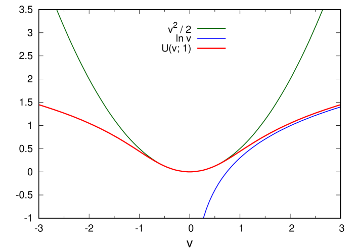
Figure 1: The weakly confining potential $U(v;v_{c})$ (1) with the controlling parameter $v_{c}=1$ (red curve). For the sake of comparison, a parabolic (green curve) and logarithmic (blue curve) potentials are also shown.

For a small $v$ much less than $v_{c}$, the potential $U(v;v_{c})$ is well approximated with $v^{2}/2$, and for a large $v$ much lager than $v_{c}$, the potential $U(v;v_{c})$ behaves as $v_{c}^{2}\ln v$, i.e.,

$$U(v;v_{c})\sim\left\{\begin{array}[]{ll}v^{2}/2,&\quad(v\ll v_{c}),\\ v_{c}^{2}\,\ln v,&\quad(v\gg v_{c}).\end{array}\right.$$ (15)

The constitutive relation for this weakly confining potential becomes

$$K(v;v_{c}):=-\alpha\frac{d}{dv}U(v;v_{c})=-\frac{\alpha v}{\sqrt{1+\left(\frac{v}{v_{c}}\right)^{4}}},$$ (16)

where $K(v;v_{c})$ is the nonlinear drift force associated with the potential $U(v;v_{c})$. From the behavior of $U(v;v_{c})$ described in Eq. (15) we see that for a small $v\ll v_{c}$ the drift force $K(v;v_{c})$ is well approximated with the linear constitutive relation $K(v;v_{c})=-\alpha v$, while for a larger $v\gg v_{c}$ $K(v;v_{c})\propto-1/v$, which means that the particle cannot be captured in the region $R_{c}$ around the minimum point of this potential $U(v;v_{c})$ if the particle velocity $v$ is much larger than $v_{c}$.

Now, we consider the canonical pdf $p(v)$ of a thermal particle in the weakly confining potential $U(v;v_{c})$,

$$p(v)\propto\exp\left[-\beta\,U(v;v_{c})\right]=\exp\left[-\beta\,\frac{v_{c}^{2}}{2}\operatorname{arsinh}\left(\frac{v^{2}}{v_{c}^{2}}\right)\right],$$ (17)

where $\beta$ is the coldness, or inverse temperature $1/(k_{\rm B}T)$. At this stage let us re-parametrize the controlling parameter $v_{c}$ as

$$\frac{v_{c}^{2}}{2}=\frac{1}{\kappa\beta},$$ (18)

where $\kappa$ is a new real parameter. With this reparametrization, the parameter $v_{c}$ is a function of $\kappa$ and $\beta$, i.e., $v_{c}=v_{c}(\kappa,\beta)$. We then find that

$$p(v) \propto\exp\left[\frac{1}{\kappa}\operatorname{arsinh}\left(-\kappa\beta\,\frac{v^{2}}{2}\right)\right]=\operatorname{\exp_{\kappa}}\left[-\beta\,\frac{v^{2}}{2}\right],$$ (19)

where we used the relation (6) in the last step. We thus see that the canonical pdf of a thermal particle in the weakly confining potential is the $\kappa$-deformed Gaussian.

Next we consider the following linear FP equation W10

$$\frac{\partial}{\partial t}p(v,t)=-\frac{\partial}{\partial v}\Big{(}K(v;v_{c})\,p(v,t)\Big{)}+D\frac{\partial^{2}}{\partial v^{2}}p(v,t),$$ (20)

where $K(v;v_{c})$ denotes the nonlinear drift coefficient in Eq. (16), and $D$ a constant diffusion coefficient. The stationary condition $\frac{\partial}{\partial t}p_{s}(v)=0$ leads to

$$\frac{\partial}{\partial v}\ln p_{s}(v) =\frac{K(v;v_{c})}{D}=-\frac{\frac{\alpha}{D}v}{\sqrt{1+\left(\frac{v}{v_{c}}\right)^{4}}}=-\frac{\alpha v_{c}^{2}}{2D}\,\frac{\partial}{\partial v}\operatorname{arsinh}\left(\frac{v^{2}}{v_{c}^{2}}\right).$$ (21)

This relation becomes

$$\ln p_{s}(v) =\frac{\alpha v_{c}^{2}}{2D}\,\operatorname{arsinh}\left(-\frac{v^{2}}{v_{c}^{2}}\right)+\textrm{const.}$$ (22)

We thus obtain the stationary pdf of the FP equation (20) as

$$p_{s}(v) \propto\exp\left[\frac{\alpha v_{c}^{2}}{2D}\operatorname{arsinh}\left(-\frac{v^{2}}{v_{c}^{2}}\ \right)\right].$$ (23)

Next we introduce the parameters as

$$\kappa=\frac{2D}{\alpha v_{c}^{2}},\quad\beta=\frac{\alpha}{D},$$ (24)

which are consistent with the relation (18). Rewriting Eq. (23) by using these parameters, we have

$$p_{s}(v) =\frac{1}{Z(\beta)}\exp\left[\frac{1}{\kappa}\operatorname{arsinh}\left(-\kappa\,\beta\,\frac{v^{2}}{2}\right)\right]=\frac{1}{Z(\beta)}\operatorname{\exp_{\kappa}}\left(-\beta\,\frac{v^{2}}{2}\right),$$ (25)

which is the $\kappa$-deformed Gaussian. In this analysis it is remarkable that: i) as shown in Eq. (24), the deformed parameter $\kappa$ is expressed in terms of the microscopic physical parameters $\alpha,D$ and the controlling parameter $v_{c}$ which determines the nonlinear constitutive relation (16). In the limit of $v_{c}\to\infty$ the deformed parameter $\kappa$ reduces to $0$; ii) the parameter $\beta$ is expressed as the ratio of the friction coefficient $\alpha$ to the diffusion coefficient $D$, in analogy with the fluctuation-dissipation relation; iii) for the region $\kappa>2$ of the deformed parameter $\kappa$, the integral $\int dvp_{s}(v)$ diverges, and consequently $p_{s}(v)$ is no longer a pdf since it cannot be normalized. By using the above parameters (24), this condition is equivalently expressed as $v_{c}^{2}<k_{B}T=1/\beta=D/\alpha$, which physically means the captured energy $v_{c}^{2}/2$ of the weakly confining potential $U(v;v_{c})$ at $v=v_{c}$ is smaller than the mean thermal energy $k_{B}T/2$. Then a thermal particle which has an enough high thermal energy cannot be captured in the region $R_{c}$ around the minimum of $U(v;v_{c})$. In other words, for a fixed value of $v_{c}$, only the limited value $\beta>1/v_{c}^{2}$ of $\beta$ is allowed for convergence of the pdf $p_{s}(v)$; iv) in the deformed parameter region $2/3<\kappa$, the second moment

$$\left\langle v^{2}\right\rangle=\int dv\,v^{2}p_{s}(v),$$ (26)

of the $\kappa$-Gaussian becomes infinite, in which the mean kinetic energy $\left\langle v^{2}\right\rangle/2$ diverges, and it is a hall-mark of anomalous transport. We will discuss this point later.

By introducing the Lyapunov functional ${\mathcal{F}[p]}$ as

$${\mathcal{F}[p]} \equiv U[p]-\frac{D}{\alpha}\,S^{\rm BG}[p],$$ (27)

with

$$S^{\rm BG}[p] =-\int dv\;p(v,t)\ln p(v,t),$$ (28)

$$U[p] \equiv\int dv\;U(v;v_{c})\,p(v,t),$$ (29)

we show W10 that

$$\frac{d{\mathcal{F}}}{dt} =\int dv\;\frac{\partial}{\partial p}\left[U(v;v_{c})\,p+\frac{D}{\alpha}\,p\ln p\right]\;\frac{\partial p}{\partial t}$$

$$=\int dv\;\left[U(v;v_{c})+\frac{D}{\alpha}\,(\ln p+1)\right]\frac{\partial}{\partial v}\,\left[-K(v;v_{c})p+D\frac{\partial p}{\partial v}\right]$$

$$=-\int dv\,\frac{p}{\alpha}\left[-K(v;v_{c})+D\,\frac{\partial}{\partial p}\ln p\right]^{2}\leq 0,$$ (30)

which states the time evolution of ${\mathcal{F}}[p]$ is non-increasing, i.e., ${\mathcal{F}}[p]$ is the Lyapunov functional w.r.t. the FP equation (20). Consequently the ${\mathcal{F}}[p]$ is minimized by the stationary solution, which is a $\kappa$-generalized Gaussian.

Having described the FP analysis of a thermal particle in the weakly confining potential $U(v;v_{c})$, we next point out the violation of the standard formula

$$\left\langle U(v)\right\rangle=-\frac{\partial}{\partial\beta}\ln Z(\beta),$$ (31)

on the average energy for a canonical pdf. It is well known that the average energy $\left\langle U(v)\right\rangle$ for a canonical pdf

$$p(v)=\frac{1}{Z(\beta)}\,\exp\left[-\beta U(v)\right],$$ (32)

is obtained by the famous relation (31). In the derivation of this formula we assume that a potential $U(v)$ is independent of $\beta$. However this assumption is no longer valid for the weakly confining potential $U(v;v_{c})$, since $v_{c}=v_{c}(\kappa,\beta)$ is a function of $\kappa$ and $\beta$. This weakly confining potential $U(v;v_{c})$ depends not only on $v$ but also on $\beta$; in other words, $U(v;v_{c})$ is temperature dependent. Consequently the above formula (31) is no longer valid. Taking into account the $\kappa$- and $\beta$-dependence of $v_{c}$, we can obtain

$$\int dv\,\frac{v^{2}}{2}\frac{p_{s}(v)}{\sqrt{1+\left(\frac{v}{v_{c}}\right)^{4}}}=-\frac{\partial}{\partial\beta}\ln Z(\beta),$$ (33)

by the straightforward calculations. The r.h.s. can be easily calculated by using the expression (25) and the analytical expression K02 for the $\kappa$-deformed Gaussian integral, as follows

$$Z(\beta) =\int_{-\infty}^{\infty}dv\,\operatorname{\exp_{\kappa}}(-\beta\frac{v^{2}}{2})$$

$$=\sqrt{\frac{\pi}{\beta\kappa}}\,\frac{\Gamma(\frac{1}{2\kappa}-\frac{1}{4})}{(1+\frac{\kappa}{2})\Gamma(\frac{1}{2\kappa}+\frac{1}{4})}\;\underset{\kappa\to 0}{\longrightarrow}\;\sqrt{\frac{2\pi}{\beta}}.$$ (34)

Then

$$-\frac{\partial}{\partial\beta}\ln Z(\beta)=\frac{\partial}{\partial\beta}\ln\sqrt{\beta}=\frac{1}{2\beta}.$$ (35)

The l.h.s. of Eq. (33) is the half of the following average energy

$$\left\langle v\frac{d}{dv}U(v;v_{c})\right\rangle =\int_{-\infty}^{\infty}dv\,\frac{v^{2}}{\sqrt{1+\left(\frac{v}{v_{c}}\right)^{4}}}\,p_{s}(v).$$ (36)

By using the relation

$$-\frac{1}{\beta}\frac{d}{dv}\,\operatorname{\exp_{\kappa}}\left(-\beta\frac{v^{2}}{2}\right)=\frac{v\operatorname{\exp_{\kappa}}\left(-\beta\frac{v^{2}}{2}\right)}{\sqrt{1+\left(\frac{v}{v_{c}}\right)^{4}}},$$ (37)

and integration by part, the r.h.s. of Eq. (36) becomes

$$-\frac{v}{\beta Z(\beta)}\operatorname{\exp_{\kappa}}\left(-\beta\frac{v^{2}}{2}\right)\Big{|}_{-\infty}^{\infty}+\frac{1}{\beta}\int_{-\infty}^{\infty}dv\,p_{s}(v).$$ (38)

Finally, let us consider the case in the parameter region $2/3<\kappa<2$, in which the second moment $\left\langle v^{2}\right\rangle$ of the $\kappa$-deformed Gaussian diverges as stated before. In this parameter region, the first term in (38) becomes zero and the stationary pdf $p_{s}(v)$ is normalized, we then obtain

$$\left\langle v\frac{d}{dv}U(v;v_{c})\right\rangle=\frac{1}{\beta}=\frac{D}{\alpha},$$ (39)

which reminds us of a generalization of equipartition theorem To ,

$$\left\langle p\frac{\partial}{\partial p}\mathcal{H}\right\rangle=k_{\rm B}T,$$ (40)

where $\mathcal{H}$ is the Hamiltonian of a system in thermal equilibrium with the temperature $T$, and $p$ is a generalized momentum conjugate w.r.t a generalized position $q$. Thus, while the mean kinetic energy diverges, the average energy (36) remains finite and is characterized by the ratio $D/\alpha$ of the diffusion coefficient $D$ to the drift coefficient $\alpha$. We note that the average energy (36) is characterized with the so called un-normalized $\kappa$-escort expectation, or $\kappa$-canonical expectation MW15 , which is written in our model by

$${\rm E}_{\kappa,p}[f(v)] :=\int dv\;f(v)\frac{d}{dx}\operatorname{\exp_{\kappa}}(x)\Big{|}_{x=-\beta\frac{v^{2}}{2}}$$

$$=\int dv\;f(v)\frac{\operatorname{\exp_{\kappa}}\left(-\beta\frac{v^{2}}{2}\right)}{\sqrt{1+\kappa^{2}\beta^{2}(v^{2}/2)^{2}}}=\int dv\;f(v)\frac{\operatorname{\exp_{\kappa}}\left(-\beta\frac{v^{2}}{2}\right)}{\sqrt{1+\left(\frac{v}{v_{c}}\right)^{4}}},$$ (41)

where we used relation (8). Then, the $\kappa$-canonical expectation of the kinetic energy $v^{2}/2$ is expressed as

$${\rm E}_{\kappa,p}\left[\frac{v^{2}}{2}\right] =\int dv\;\frac{v^{2}}{2}\;\frac{Z(\beta)p_{s}(v)}{\sqrt{1+\left(\frac{v}{v_{c}}\right)^{4}}}=-\frac{\partial}{\partial\beta}Z(\beta),$$ (42)

where the relation (33) was used in the last step. In the limit of $\kappa\to 0$, the relation (42) reduces to the standard relation

$$Z(\beta)\left\langle\frac{v^{2}}{2}\right\rangle=-\frac{\partial}{\partial\beta}Z(\beta).$$ (43)

4 Conclusion and perspective

We have considered a thermal particle in a weakly confining potential $U(v;v_{c})$ in $v$-space with a control parameter $v_{c}$. We have shown that its stationary state is a canonical probability distribution which is the $\kappa$-deformed Gaussian. In this model the parameter $v_{c}$ characterizes the $v$-dependency of the weakly confining potential $U(v;v_{c})$, and consequently determines the nonlinear constitutive relation (16). Then, the deformed parameter $\kappa$ is determined by $v_{c}$ and $\beta$ as shown in relations (24). In this way, we provide a possible physical meaning of the deformed parameter $\kappa$ in this model. Note also that our nonlinear velocity-dependent potential $U(v;v_{c})$ can be considered as a generalization of Rayleigh dissipation function with the deformed parameter $v_{c}$.

Recently, Chaudhuri Chaudhuri discussed the stochastic dynamics of the active Brownian particles which are modeled in terms of nonlinear velocity dependent force. Using the associated FP equation, he derived the expression for the total entropy production. Since our model is also described by the nonlinear velocity dependent force, it is worth to further study our model from the view of the entropy production and associated fluctuation theorem.

It is interesting to further study the relation (42) from the view points of both statistical physics and Information geometry.

Another possible further study is to generalize our model by utilizing Naudts’ $\phi$-exponential function Naudts . It is a unification of some deformed-exponential functions. It includes the $q$- and $\kappa$-exponential functions as special cases. The inverse function of the $\phi$-exponential function is called $\phi$-logarithmic function, which is defined by

$$\ln_{\phi}(x)\equiv\int_{1}^{x}\frac{ds}{\phi(s)},$$ (44)

for a positive increasing function $\phi(s)$. The $\kappa$-logarithm is a special case of Naudt’s $\phi$-logarithm with

$$\phi(s)=\frac{2s}{s^{\kappa}+s^{-\kappa}}.$$ (45)

References

- (1) Strutt, J. W. (Lord Rayleigh): Some general theorems relating to vibrations. Proc. London Math. Soc. s1-4, 357-368, (1871)
- (2) Wada, T.,: A nonlinear drift which leads to -generalized distribution. Eur. Phys. J. B 73 287-291 (2010)
- (3) Lutz, E., Renzoni, F.: Beyond Boltzmann-Gibbs statistical mechanics in optical lattices. Nature Physics, 9, 615-619 (2013)
- (4) Scarfone, A.M., Wada, T.: Legendre structure of -thermostatistics revisited in the framework of information geometry. J. Phys. A: Math. Theor. 47, 275002 (2014)
- (5) Wada, T., Scarfone, A.M.: Information geometry on the -thermostatistics. Entropy 17, 1204-1217 (2015)
- (6) Wada, T., Matsuzoe, H., Scarfone, A.M.: Dualistic Hessian structures among the thermodynamic potentials in the -thermostatistics. Entropy 17, 7213-7229 (2015)
- (7) Scarfone, A.M., Matsuzoe, H., Wada, T.: Information Geometry of -Exponential Families: Dually-Flat, Hessian and Legendre Structures. Entropy 20, 436 (2018)
- (8) Amari, S-I.: Information Geometry and Its Applications. Springer: Tokyo, Japan, (2016)
- (9) Tsallis, C.: Introduction to Nonextensive Statistical Mechanics. Approaching a Complex World. Springer: NY, USA, (2009)
- (10) Kaniadakis, G., Scarfone, A.M.: A new one-parameter deformation of the exponential function. Physica A, 305, 69-75 (2002)
- (11) Kaniadakis, G.: Statistical mechanics in the context of special relativity. Phys. Rev. E 66, 056125 (2002)
- (12) Kaniadakis, G.: Statistical mechanics in the context of special relativity II. Phys. Rev. E 72, 036108 (2005)
- (13) Kaniadakis, G.: Theoretical foundations and mathematical formalism of the power-law tailed statistical distributions. Entropy, 15, 3983-4010 (2013)
- (14) Scarfone, A. M.: On the, kappa-Deformed Cyclic Functions and the Generalized Fourier Series in the Framework of the kappa-Algebra. Entropy, 17, 2812-2833 (2015)
- (15) Scarfone, A. M.: -deformed Fourier transform. Physica A, 480, 63-78 (2017)
- (16) Kaniadakis, G., Scarfone, A. M., Sparavigna, A., Wada, T.: Composition law of -entropy for statistically independent systems. Phys. Rev. E 95, 052112 (2017)
- (17) Tolman, R. C.: A General Theory of Energy Partition with Applications to Quantum Theory. Phys. Rev. 11, 261-275, (1918)
- (18) Matsuzoe, H., Wada, T.: Deformed Algebras and Generalizations of Independence on Deformed Exponential Families. Entropy 17, 5729-5751 (2015)
- (19) Chaudhuri, D.: Entropy production by active particles: Coupling of odd and even functions of velocity. Phys. Rev. E 94, 032603 (2016)
- (20) Naudts, J.: Generalized Thermostatistics. Springer: Berlin, Germany, (2011)