Weakly-Convex Concave Min-Max Optimization: Provable Algorithms and Applications in Machine Learning
Abstract
Min-max problems have broad applications in machine learning, including learning with non-decomposable loss and learning with robustness to data distribution. Convex-concave min-max problem is an active topic of research with efficient algorithms and sound theoretical foundations developed. However, it remains a challenge to design provably efficient algorithms for non-convex min-max problems with or without smoothness. In this paper, we study a family of non-convex min-max problems, whose objective function is weakly convex in the variables of minimization and is concave in the variables of maximization. We propose a proximally guided stochastic subgradient method and a proximally guided stochastic variance-reduced method for the non-smooth and smooth instances, respectively, in this family of problems. We analyze the time complexities of the proposed methods for finding a nearly stationary point of the outer minimization problem corresponding to the min-max problem.
keywords:
min-max optimization, non-smooth optimization; stochastic optimization; non-convex optimization1 Introduction
The goal of this paper is to design provably efficient algorithms for solving min-max (aka saddle-point) problems of the following form:
| (1) |
where is continuous, and and are proper and closed.111A closed function can be also called a lower semi-continuous function. Detailed assumptions (e.g. weak convexity) on , and will be given in Assumptions 1, 2 and 3. Many machine learning tasks can be formulated as (1) and some applications are given in Section 1.1. Although there exist many studies on min-max problems in the form of (1), most of them focus on convex-concave problems, where both and are convex and is convex in given and is concave in given . On the contrary, this paper focuses on developing provably efficient algorithms for (1) that exhibits non-convexity in .
When designing an algorithm for (1) with non-convexity, the important questions are what type of solutions can the algorithm guarantees and what runtime the algorithm needs to find such solutions. In the recent studies on non-convex minimization [9, 8, 7, 10, 13, 12, 15, 16, 18, 29, 31, 32], polynomial-time algorithms have been developed for finding a nearly stationary point, namely, a point close to another point where the subdifferential of objective function almost contains zero. However, these developments are for a general minimization problem without utilizing the max-structure in (1) when it arises, and thus are not directly applicable to (1). For example, the method in [10] required that a stochastic subgradient of is available at each iteration. This might not be true if the maximization over in (1) is non-trivial or if is given as an expectation.
To fill this gap, in this paper, we analyze the complexity of a first-order algorithm designed to find a nearly stationary point of in (1) without solving the possibly complex inner maximization problem exactly for each . We focus on a typical case of (1) that is non-convex but weakly convex in and is concave in . We refer to this case of (1) as a weakly-convex-concave (WCC) min-max problem. We provide complexity analysis for two primal-dual stochastic first-order methods under different settings of . We will discuss some important applications of WCC min-max problems in machine learning next and summarize our main contributions at the end of this section.
1.1 Applications Of WCC Min-Max Problem
Distributionally robust learning. [25] formulates the problem of distributionally robust learning as
| (2) |
where denotes the loss of a model on the th data point, , is a closed convex set, and is a closed convex function, e.g., for some , where is an all-one vector and denotes some distance measure (e.g., KL divergence and Euclidean distance) between two vectors. The loss can be a non-convex function such as the loss function defined by a neural network or the non-convex truncated loss [39]. It is easy to see that (2) is a special case of (1).
Learning with non-decomposable loss. Problem (1) also covers some models where the objective function cannot be represented as a summation of the losses over a training set. One example is minimizing the sum of top- losses [14, 11]:
where is a permutation of such that . When , it reduces to the minimization of maximum loss [34]. This problem can be reformulated as the form (1) according to [3] and [11] and our methods can be applied even if is non-convex.
Robust learning from multiple distributions. Let denote distributions of data, e.g., different perturbed versions of the underlying true distribution . Robust learning from multiple distributions is to minimize the maximum of the expected losses over the distributions, i.e.,
| (3) |
where , is a non-convex loss function (e.g., the loss defined by a deep neural network) of a model parameterized by on an example , and denotes the expected loss on distribution . It is an instance of (1) that is non-convex in and concave in . Such a formulation also has applications in adversarial machine learning [24, 37], in which corresponds to a distribution used to generate adversarial examples.
1.2 Contributions
Despite the concavity of in , there still remain challenges in developing provably efficient algorithms for (1) due to the non-convexity of in . The major contribution of this work is the development and analysis of two efficient stochastic algorithms for the WCC min-max problem (1) without evaluating the maximization in (1) exactly at each iteration. We establish the convergence of the proposed algorithms to a nearly stationary point of . The main key assumption we make is that is weakly convex in and concave in . We summarize our contributions as follows.
-
•
When is potentially non-smooth and given as the expectation of a stochastic function, we present a stochastic primal-dual subgradient algorithm for (1). This method achieves time complexity of for finding a nearly -stationary solution. 222Here and in the rest of the paper, suppresses all logarithmic factors.
-
•
When is strongly convex and can be represented as the average of potentially non-smooth functions linear in (see D2 in Assumption 2), the complexity of our method can be improved to . To the best of our knowledge, this is the first result on accelerating a stochastic primal-dual subgradient algorithm for a non-convex and non-smooth min-max problem under strong concavity.
-
•
When is represented as the average of smooth functions, we present a stochastic variance-reduced gradient method for (1). When is strongly convex, our method has time complexity of for finding a nearly -stationary solution. When is convex, this method has time complexity of .
2 Related Work
Recently, there is a growing interest in stochastic algorithms for non-convex optimization. When the objective function is smooth, stochastic gradient descent [15] and its variants [40, 16] have been analyzed for finding a stationary point of the objective function. When the objective function has a finite-sum structure, accelerated stochastic algorithms with improved complexity have been developed based on the variance reduction techniques [32, 31, 18, 1, 2]. However, these methods are not directly applicable to (1) because of the non-smoothness of .
Several recent papers have proposed algorithms and provided theoretical guarantees for non-convex optimization with non-smooth objective functions by assuming the objective function is weakly convex [8, 9, 12, 10, 6, 41]. Although the objective function in our problem is also weakly convex, most of the aforementioned methods cannot be directly applied to (1) because they need to compute the (stochastic) subgradient of which requires exactly solving the concave maximization problem that can be challenging, e.g., when involves expectations as in (3).
The following weakly convex composite optimization has been studied by [12],
| (4) |
where is closed and convex, is Lipschitz-continuous and convex and is smooth with a Lipschitz-continuous Jacobian matrix. It is a special case of (1) because we can reformulate (4) as
| (5) |
where is the conjugate of . [12] proposed a prox-linear method for (4) where the iterate is updated by approximately solving
| (7) |
Here, is the Jacobian matrix of and is a step length. They considered using accelerated gradient method to solve (7). However, this approach requires the exact evaluation of and which is computationally expensive, for example, when is given as an expectation or a finite sum of many terms (see (2) and (3)). One approach to avoid this issue is to solve (7) as a min-max subproblem
| (10) |
using primal-dual stochastic first-order methods that only require the sample approximation of and . However, they still require to be smooth to ensure the convergence of . In contrast, our convergence analysis covers the case where is non-smooth.
The authors of [5] considered robust learning from multiple datasets to tackle uncertainty in the data, which is a special case of (3). They assumed that the minimization over for any fixed can be solved up to a certain optimality gap relative to the global minimum value. However, such an assumption does not hold when the minimization over is non-convex. [30] considered a similar problem to (3) and analyzed a primal-dual stochastic algorithm. There are several differences between their results and ours: (i) they require to be smooth while we assume it is weakly convex but not necessarily smooth; (ii) they proved the convergence of the partial gradient of with respect to while we provide the convergence of the gradient of the Moreau envelope of ; (iii) when is smooth and has a finite-sum structure, we provide an accelerated stochastic algorithm based on variance reduction which they did not consider. [38, 22, 23, 27] propose deterministic algorithms for a problem similar to (1) and [20, 4] consider both deterministic and stochastic methods for (1). These studies, except [4], all assume is smooth, and [27] further assume satisfies the Polyak-Lojasiewicz condition in . On the contrary, our results cover the case where is non-smooth and, without strong concavity in , our stochastic algorithm has lower complexity than [20, 4]. In particular, the complexity of our method for finding a nearly -stationary point is without strong concavity while the complexity of [20, 4] is .
3 Preliminaries
We consider the min-max problem (1) where is continuous, and are proper and closed. According to most of the applications of (1) (see Section 1.1), the roles of and are often not symmetric, e.g., are often restricted to a simplex in but are not. Hence, we only equip with the Euclidean norm but equip with a generic norm so that the algorithm can better adapt to the geometry of the feasible set of . We denote the dual norm of by and define for any set .
Given , the subdifferential of is
where each element in is called a subgradient of at . Let be the subdifferential of with respective to and be the subdifferential of with respective to .
Let
Let be a distance generating function with respect to , meaning that is convex on , continuously differentiable and -strongly convex with respect to on . The Bregman divergence associated to is defined as such that
| (11) |
Note that we have . We say a function is -strongly convex () with respect to if
for any and any . We say a function is -weakly convex () if
for any and any .
The following assumptions are made throughout the entire paper:
Assumption 1.
The following statements hold:
-
(A)
is -weakly convex in for any .
-
(B)
is concave in for any .
-
(C)
is closed and -strongly convex with respect to with ( can be zero) and is closed and convex.
-
(D)
.
Under Assumption 1, is -weakly convex (but not necessarily convex) so that finding the global optimal solution in general is difficult. An alternative goal is to find a stationary point of (1), i.e., a point with . An exact stationary point, in general, can only be approached in the limit as the number of iterations increases to infinity. Within finitely many iterations, a more reasonable goal is to find an -stationary point defined below.
Definition 3.1.
A point is an -stationary point if .
However, when is non-smooth, computing an -stationary point is still difficult even for a convex problem. A simple example is where the only stationary point is but is not an -stationary point with no matter how close is to . This situation is likely to occur in problem (1) because of not only the potential non-smoothness of and but also the inner maximization. Therefore, following [8], [10], [7] and [41], we consider the Moreau envelope of defined as
| (12) |
for a constant . For a -weakly convex function , it can be shown that is smooth when [10] and its gradient is
| (13) |
where
Note that, when , the minimization in (12) and (13) is strongly convex so that is uniquely defined. We then give the following definition
Definition 3.2.
A point is a nearly -stationary point if .
According to [8], [10], [7] and [41], the norm of the gradient can be used as a measure of the quality of a solution . In fact, let . The definition (13) and the optimality condition of directly imply that
Therefore, if we can find a nearly -stationary point , we will ensure and , or in other words, we will find a solution that is -closed to -stationary point (i.e., ). Hence, we will focus on developing first-order methods for (1) and analyze their time complexity for finding a nearly -stationary point.
4 Proximally Guided Approach
The method we proposed is largely inspired by the proximally guided stochastic subgradient method by [10], which is a variant of the inexact proximal point method [33]. [10] considers with being a -weakly convex function that does not necessarily have the maximization structure in (1). Given an iterate , their method uses the standard stochastic subgradient (SSG) method to approximately solve (12) with and , namely, to compute a solution so that
| (14) |
Then returned by the SSG method will be used as the next iterate. They assume that a (stochastic) subgradient of can be computed during the SSG method, which does not hold in our setting due to the maximization in (1).
To address this issue, we consider the following min-max problem according to (14):
| (15) |
and equivalently solve (14) as
| (16) |
Existing primal-dual first-order methods can be applied to (15), or specifically, (16), and the returned approximate solution is then used as the next iterate. In this section, we will consider two cases for : when is given as an expectation and potentially non-smooth, and when is a finite sum and smooth.
For a non-smooth min-max problem, strong convexity and strong concavity are simultaneously needed to accelerate a primal-dual first-order method. Under Assumption 1, when , is -strongly convex in and -concave with respect to in . Although a deterministic primal-dual method for (16) with a non-smooth can be accelerated when , it is surprising that there is no existing stochastic primal-dual methods that can be accelerated when . In Section 4.1, we propose a new stochastic primal-dual method for (1) whose complexity for finding a nearly -stationary point can be improved from when to when under a structural assumption (D2 in Assumption 2). This is the first stochastic algorithm for non-smooth non-convex min-max problems that can be accelerated under strong concavity.
4.1 Stochastic Min-Max Problem
In this section, we make the following assumptions in addition to Assumption 1.
Assumption 2.
The following statements hold:
-
(A)
For any , we can compute two random vectors, denoted by and , such that .
-
(B)
There exist constants and such that and for any .
-
(C)
and .
-
(D)
Either one of the following two statements holds:
-
D1.
; ; and .
-
D2.
; where is -weakly convex in for any ; and satisfies for some and any and in . Moreover, and in Assumption 2 (A) above satisfy and , where is a uniformly random index from .
-
D1.
We propose a proximally guided stochastic mirror descent (PG-SMD) method for (1) in Algorithms 1 and 2. Algorithm 2 is the main algorithm which, in its th iteration, uses Algorithm 1 to approximately solve (16). The returned solution will be used as the th iterate of Algorithm 2. Algorithm 1 is exactly the primal-dual SMD method [26] applied to (15). It is initialized at where when Assumption 2 D1 holds and when Assumption 2 D2 holds. Assumption 2 D2 (i.e., is linear in ) ensures this maximization can be solved easily, for example, in a closed form. We emphasize that such an initialization of in the case of D2 is the key to utilize the strong concavity of in to reduce the complexity from when to when .
Theorem 4.1 characterizes the time complexity for PG-SMD to find a nearly -stationary point. We define the time complexity as the total number of the stochastic subgradients calculated and we count the complexity of solving in case D2 as computing stochastic subgradients. The proof and the exact expressions of are provided in Section A in Appendix.
4.2 Smooth Finite-Sum Min-Max Problem
In this section, we no longer need Assumption 2 but make the following assumption in addition to Assumption 1.
Assumption 3.
The following statements hold:
-
(A)
with .
-
(B)
is differentiable with -Lipschitz continuous and -Lipschitz continuous. 333 and are the partial gradients of with respect to and , respectively.
-
(C)
and .
Different from the previous section, we can exactly evaluate but the computational cost can be still high when is large. To reduce the cost, in Algorithm 3 and Algorithm 4, we propose a proximally guided stochastic variance-reduced gradient (PG-SVRG) method for (1). We consider a min-max problem
| (17) |
where and is defined in (15). Given the current iterate , Algorithm 4 applies Algorithm 3, which is the stochastic variance-reduced gradient (SVRG) method [28, 35], to approximately solve
| (18) |
with some and for any . The returned solution will be used as the next iterate. Compared to (15), problem (17) has an additional proximal term introduced to make (17) strongly convex and strongly concave so that (18) can be solved efficiently with the SVRG method. When is already strongly concave with respect to , we will set for any and follow the convention that so that will be removed from (18) and thus (18) is reduced to (16).
Theorem 4.2 characterizes the time complexity for PG-SVRG to find a nearly -stationary point. We define the time complexity as the total number of the stochastic gradients calculated and count the complexity of computing as computing stochastic gradients. The proof and the exact expressions of are provided in Section B in Appendix.
Theorem 4.2.
5 Numerical Experiments
In this section, we present numerical experiments to demonstrate the performance of our proposed methods. We first consider the distributionally robust learning problem in (2) with smooth and non-smooth loss function ’s. Then, we will test the algorithms on the robust learning problem from multiple distributions (3) with non-smooth losses.
5.1 Robust Learning with Smooth Loss
In this section, we consider learning from imbalanced data by solving the robust learning problem in (2) with and , where is the KL-divergence between two vectors in the simplex . We conduct two experiments with different non-convex smooth losses ’s in (2).
In the first experiment, we learn a linear model with the loss formed by truncating the logistic loss for binary classification, i.e., where denotes the feature vector, denotes its binary class label for , , and for . A truncated loss makes it robust to outliers and noisy data [21, 39], though it is not our goal to demonstrate the benefit of using truncation here. For this experiment, we focus on comparison with two baseline methods for solving (2). Note that (2) is also a special case of (4) with and . Hence, we compare our method with the proximal linear (PL) method [12] that solves (4) using the updating scheme (7). [12] suggested using the accelerated gradient method to solve (7) which has a high computational cost when is large. Hence, we also use the SMD and SVRG methods to solve (7) to reduce the complexity of the PL method through sampling . We denote the PL methods using the SMD and SVRG methods to solve (7) as PL-SMD and PL-SVRG, respectively.
| Datasets | #Train | #Test | #Feat. | - : + |
|---|---|---|---|---|
| covtype | 217594 | 30000 | 54 | 1:7.5 |
| connect-4 | 29108 | 32000 | 126 | 1:5.3 |
| protein | 10263 | 4298 | 357 | 1:4.0 |
| rcv1.binary | 12591 | 677399 | 47236 | 1:5.1 |
We perform the comparisons on four imbalanced datasets from the LIBSVM library. Table 1 contains information about the four datasets used in the experiments. The information includes the sizes of training and testing sets, the number of features, and the ratio of negative instances to positive instances in training sets (testing tests are almost balanced). For datasets covtype and connect-4, we selected two imbalanced classes from the original data and split them appropriately into imbalanced training and balanced testing sets. Datasets protein and rcv1.binary were already split into training and testing sets, so we select two classes and randomly removed some negative instances from the training sets to make them imbalanced.
In this experiment, we set . Mini-batches of size , , , and were chosen for protein, rcv1.binary, connect-4, and covtype, repectively, when we compute stochastic gradients in all methods. We implement PG-SMD in case D1. The values of some control parameters in the algorithms are selected from a discrete grid of candidate values using the objective value of (2) at termination as the criterion. Those control parameters include in (7) for the two PL methods, in both PG-SMG and PG-SVRG, the ratios and in the expressions of and in SMD as well as , , and in SVRG.
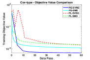
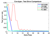
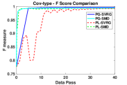
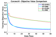
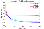
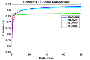
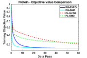
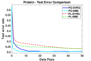
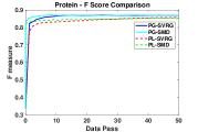
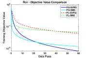
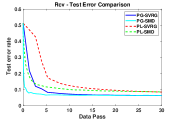
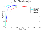
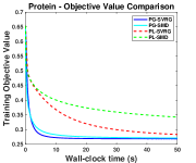
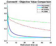
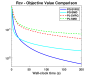
Figure 1 shows the objective value of (2), testing classification error rate and F-score as the number of data passes increases. On these datasets, the proposed PG methods are more advantageous than the PL methods. This is mainly because the gradient information (subject to stochastic noise) used in (7) in the PL methods is only updated in each outer loop while our PG methods update this in each inner loop, which ensures that the solutions are updated with the latest gradient information. Overall, PG-SVRG does well in the long run in reducing the objective value, while PG-SMD is faster in yielding a low test error rate. Additional comparisons are given in Figure 2, where we show the objective value (the training loss) obtained by the PL and PG methods at different wall-clock times in seconds. Figure 2 also shows that the PG methods are more time efficient than the PL methods.
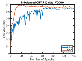
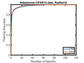
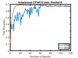
In the second experiment, we learn a non-linear model with the loss defined by a deep neural network. For this experiment, we focus on demonstrating the power of the proposed method for improving the generalization performance. We do that by solving the distributionally robust optimization (DRO) (2) in comparison with traditional empirical risk minimization (ERM) by SGD. To this end, we use an imbalanced CIFAR10 data and two popular deep neural networks (ResNet18 [17] and VGG19 [36]). The original training data of CIFAR10 has ten classes, each of which has 5000 images. We remove 4900 images from five classes to make the training set imbalanced. The test data remains intact.
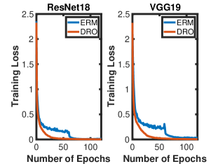
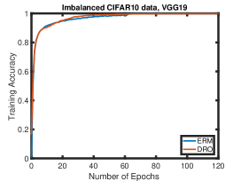
The value of is fixed to in this experiment, and the mini-batch size is fixed to 128 for both methods. We use SGD to solve ERM with a stepsize of 0.1 for epochs and for epochs following the practical training strategy [17], where one epoch means one pass of data. We implement PG-SMD in case D1 using the similar practical training strategy except that we choose , , , in epochs , , , respectively. is selected by grid search as in the first experiment. The curves for training and testing accuracy are plotted in Figure 3, which show that a robust optimization scheme is considerably better than ERM when dealing with imbalanced data in these two specific examples. Additional comparison is given in Figure 4, where we show the training loss (the objective value) obtained by the ERM and DRO methods at different epochs.
5.2 Robust Learning with Non-Smooth Loss
In this section, we perform numerical experiments on the same robust learning problem as in Section 5.1 except that we use non-smooth loss function ’s in (2) this time. In particular, we consider the loss function for binary classification defined by a two-layer fully-connected neural network where the loss in the output layer is calculated using the hinge loss. Let denote the feature vector and denote its binary class label for . Let be the number of neurons in the hidden layer and be the weights with and . Then the loss from the th data point is defined as
| (19) |
where is the component-wise sigmoid function, i.e.,
| (20) |
It can be proved that (2) with this loss function is still weakly convex in . However, since ’s are non-smooth, we cannot apply the PG-SVRG, PL-SMD, and PL-SVRG methods in the previous subsection to (2). An alternating stochastic gradient descent (Alter-SGD) method is proposed in [4], which can be applied to (2) with non-smooth ’s. Hence, we will focus on comparing PG-SMD and Alter-SGD.
We perform the comparisons on imbalanced datasets covtype and connect-4 whose construction is described in Section 5.1 and statistics can be found in Table 1. In this experiment, we set and . Mini-batches of size and were chosen for covtype and connect-4, repectively, when we compute stochastic gradients in both methods. We implement PG-SMD in case D1. The values of control parameters, including and the ratios and in PG-SMG as well as and in PG-SMD and Alter-SGD, are selected in the same way as in Section 5.1.
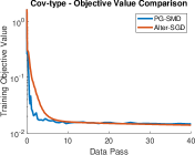
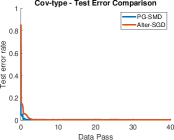
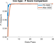
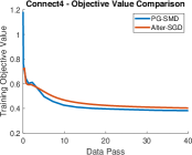
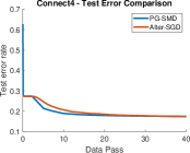
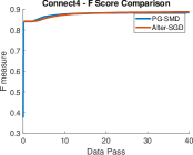
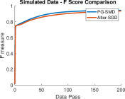
Figure 5 shows the objective value of (2), testing classification error rate and F-score as the number of data passes increases. The proposed PG-SMD method is a little more advantageous than the Alter-SGD method on these specific examples. Overall, PG-SMD reduces the objective value slightly faster than Alter-SGD when the number of data passes is small.
5.3 Robust Learning from Multiple Distribution
In this section, we present the numerical experiments on the robust learning problem from multiple distributions described in (3) with different data distributions , . We consider the case when ’s are continuous distributions and we generate ’s by simulation.
Let be a random data point from one of the five distributions, where is the feature vector and is its label. If is generated from , let the coordinates and be generated independently from a uniform distribution on , where if and if . Then let the remaining coordinates be zeros. Next, we generate the binary label corresponding to using a two-layer fully-connected neural network. To do that, we first randomly generate the true weights with and and each entry of and generated independently from a uniform distribution on . Then, we fix and, for each generated feature vector , we generate a noise from a uniform distribution on and generate the label as
With the data distribution for defined in this way, we solve (3) with and , where is defined as in (19).
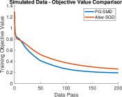
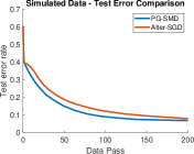
It can be proved that (3) with this loss function is weakly convex in . However, since is non-smooth and each is defined with an expectation rather than a finite sum, we cannot apply PG-SVRG or the PL methods, so we will again focus on comparing PG-SMD and Alter-SGD. A mini-batch of size was used when we compute stochastic gradients in both methods. Each sample in a mini-batch is generated using and the aforementioned procedure. The values of control parameters of both methods are selected in the same way as in Section 5.2. Besides the mini-batches used in optimization, we generate data points from each separately and use them to closely approximate the objective value of (3), testing classification error rate and F-score. These values are shown in Figure 6 as the number of data passes increases. Similar to (5), the proposed PG-SMD method is better than the Alter-SGD method in this specific example.
6 Conclusion
This paper contributes to the numerical solvers for non-convex min-max problems. We focus on a class of weakly-convex-concave min-max problems where the minimization part is weakly convex, and the maximization part is concave. This class of problems covers many important applications, such as robust learning. We consider two different scenarios: (i) the min-max objective function involves expectation, and (ii) the objective function is smooth and has a finite-sum structure. Stochastic mirror descent method and stochastic variance-reduced gradient method are developed to solve the subproblem in scenario (i) and (ii), respectively. We analyze the computational complexity of our methods for finding a nearly -stationary for the original problem under both scenarios. Numerical experiments on distributionally robust learning with non-convex losses demonstrate the effectiveness of the proposed methods.
References
- [1] Z. Allen-Zhu, Natasha: Faster Non-Convex Stochastic Optimization via Strongly Non-Convex Parameter, in Proceedings of the 34th International Conference on Machine Learning (ICML). 2017, pp. 89–97.
- [2] Z. Allen-Zhu and E. Hazan, Variance Reduction for Faster Non-Convex Optimization, in Proceedings of the 33nd International Conference on Machine Learning (ICML). 2016, pp. 699–707.
- [3] C. Bennett and R. Sharpley, Interpolation of Operators, Pure and Applied Mathematics, Elsevier Science, 1988, Available at https://books.google.com/books?id=HpqF9zjZWMMC.
- [4] R.I. Boţ and A. Böhm, Alternating proximal-gradient steps for (stochastic) nonconvex-concave minimax problems, arXiv preprint arXiv:2007.13605 (2020).
- [5] R.S. Chen, B. Lucier, Y. Singer, and V. Syrgkanis, Robust optimization for non-convex objectives, in Advances in Neural Information Processing Systems 30 (NIPS, 2017, pp. 4705–4714.
- [6] Z. Chen, Z. Yuan, J. Yi, B. Zhou, E. Chen, and T. Yang, Universal stagewise learning for non-convex problems with convergence on averaged solutions, arXiv preprint arXiv:1808.06296 (2018).
- [7] D. Davis and D. Drusvyatskiy, Complexity of finding near-stationary points of convex functions stochastically, arXiv preprint arXiv:1802.08556 (2018).
- [8] D. Davis and D. Drusvyatskiy, Stochastic subgradient method converges at the rate on weakly convex functions, arXiv preprint arXiv:1802.02988 (2018).
- [9] D. Davis and D. Drusvyatskiy, Stochastic model-based minimization of weakly convex functions, SIAM Journal on Optimization 29 (2019), pp. 207–239.
- [10] D. Davis and B. Grimmer, Proximally guided stochastic subgradient method for nonsmooth, nonconvex problems, SIAM Journal on Optimization 29 (2019), pp. 1908–1930.
- [11] O. Dekel and Y. Singer, Support Vector Machines on a Budget, in NIPS. 2006, pp. 345–352.
- [12] D. Drusvyatskiy and C. Paquette, Efficiency of minimizing compositions of convex functions and smooth maps, Mathematical Programming (2018).
- [13] D. Drusvyatskiy, The proximal point method revisited, arXiv preprint arXiv:1712.06038 (2017).
- [14] Y. Fan, S. Lyu, Y. Ying, and B. Hu, Learning with Average Top-k Loss, in Advances in Neural Information Processing Systems (NIPS). 2017, pp. 497–505.
- [15] S. Ghadimi and G. Lan, Stochastic first- and zeroth-order methods for nonconvex stochastic programming, SIAM Journal on Optimization 23 (2013), pp. 2341–2368.
- [16] S. Ghadimi and G. Lan, Accelerated gradient methods for nonconvex nonlinear and stochastic programming, Math. Program. 156 (2016), pp. 59–99.
- [17] K. He, X. Zhang, S. Ren, and J. Sun, Deep residual learning for image recognition, in Proceedings of the IEEE conference on computer vision and pattern recognition. 2016, pp. 770–778.
- [18] G. Lan and Y. Yang, Accelerated stochastic algorithms for nonconvex finite-sum and multi-block optimization, CoRR abs/1805.05411 (2018).
- [19] Q. Lin, R. Ma, and T. Yang, Level-set methods for finite-sum constrained convex optimization, in International Conference on Machine Learning. 2018, pp. 3118–3127.
- [20] T. Lin, C. Jin, and M.I. Jordan, On Gradient Descent Ascent for Nonconvex-Concave Minimax Problems, in International Conference on Machine Learning (ICML). 2020.
- [21] P.L. Loh, Statistical consistency and asymptotic normality for high-dimensional robust -estimators, The Annals of Statistics 45 (2017), pp. 866–896. Available at https://doi.org/10.1214/16-AOS1471.
- [22] S. Lu, I. Tsaknakis, and M. Hong, Block alternating optimization for non-convex min-max problems: algorithms and applications in signal processing and communications, in Proceedings of IEEE International Conference on Acoustics, Speech and Signal Processing (ICASSP). 2019.
- [23] S. Lu, I. Tsaknakis, M. Hong, and Y. Chen, Hybrid block successive approximation for one-sided non-convex min-max problems: algorithms and applications, IEEE Transactions on Signal Processing (2020).
- [24] A. Madry, A. Makelov, L. Schmidt, D. Tsipras, and A. Vladu, Towards deep learning models resistant to adversarial attacks, arXiv preprint arXiv:1706.06083 (2017).
- [25] H. Namkoong and J.C. Duchi, Variance-based Regularization with Convex Objectives, in Advances in Neural Information Processing Systems (NIPS). 2017, pp. 2975–2984.
- [26] A. Nemirovski, A. Juditsky, G. Lan, and A. Shapiro, Robust stochastic approximation approach to stochastic programming, SIAM Journal on Optimization 19 (2009), pp. 1574–1609.
- [27] M. Nouiehed, M. Sanjabi, T. Huang, J.D. Lee, and M. Razaviyayn, Solving a class of non-convex min-max games using iterative first order methods, in Advances in Neural Information Processing Systems. 2019, pp. 14934–14942.
- [28] B. Palaniappan and F. Bach, Stochastic Variance Reduction Methods for Saddle-Point Problems, in Advances in Neural Information Processing Systems. 2016, pp. 1408–1416.
- [29] C. Paquette, H. Lin, D. Drusvyatskiy, J. Mairal, and Z. Harchaoui, Catalyst for Gradient-based Nonconvex Optimization, in International Conference on Artificial Intelligence and Statistics. 2018, pp. 613–622.
- [30] Q. Qian, S. Zhu, J. Tang, R. Jin, B. Sun, and H. Li, Robust optimization over multiple domains, in Proceedings of the AAAI Conference on Artificial Intelligence, Vol. 33. 2019, pp. 4739–4746.
- [31] S.J. Reddi, A. Hefny, S. Sra, B. Póczós, and A. Smola, Stochastic Variance Reduction for Nonconvex Optimization, in Proceedings of the 33rd International Conference on International Conference on Machine Learning (ICML). JMLR.org, 2016, pp. 314–323.
- [32] S.J. Reddi, S. Sra, B. Póczos, and A.J. Smola, Fast incremental method for smooth nonconvex optimization, in 55th IEEE Conference on Decision and Control (CDC). 2016, pp. 1971–1977.
- [33] R.T. Rockafellar, Monotone operators and the proximal point algorithm, SIAM J. on Control and Optimization 14 (1976). Available at http://epubs.siam.org/sicon/resource/1/sjcodc/v14/i5/p877_s1.
- [34] S. Shalev-Shwartz and Y. Wexler, Minimizing the Maximal Loss: How and Why, in Proceedings of the 33nd International Conference on Machine Learning, ICML 2016, New York City, NY, USA, June 19-24, 2016. 2016, pp. 793–801. Available at http://jmlr.org/proceedings/papers/v48/shalev-shwartzb16.html.
- [35] Z. Shi, X. Zhang, and Y. Yu, Bregman divergence for stochastic variance reduction: saddle-point and adversarial prediction, in Advances in Neural Information Processing Systems. 2017, pp. 6031–6041.
- [36] K. Simonyan and A. Zisserman, Very deep convolutional networks for large-scale image recognition, arXiv preprint arXiv:1409.1556 (2014).
- [37] A. Sinha, H. Namkoong, R. Volpi, and J. Duchi, Certifying some distributional robustness with principled adversarial training, arXiv preprint arXiv:1710.10571 (2017).
- [38] K.K. Thekumparampil, P. Jain, P. Netrapalli, and S. Oh, Efficient algorithms for smooth minimax optimization, in Advances in Neural Information Processing Systems. 2019, pp. 12680–12691.
- [39] Y. Xu, S. Zhu, S. Yang, C. Zhang, R. Jin, and T. Yang, Learning with non-convex truncated losses by SGD, in Uncertainty in Artificial Intelligence. PMLR, 2020, pp. 701–711.
- [40] T. Yang, Q. Lin, and Z. Li, Unified convergence analysis of stochastic momentum methods for convex and non-convex optimization, arXiv preprint arXiv:1604.03257 (2016).
- [41] S. Zhang and N. He, On the convergence rate of stochastic mirror descent for nonsmooth nonconvex optimization, arXiv preprint arXiv:1806.04781 (2018).
Appendix A Proof of Theorem 4.1
We first present the convergence result of SMD for solving (15) proved by [26]. The proof is well-known and included only for the sake of completeness.
Proposition A.1 (Convergence of Algorithm 1).
Proof.
For simplicity of notation, we write as in this proof and define
Next, we will perform the standard analysis of SMD (e.g. the proof of Proposition 3.2 in [26]). According to the updating equations of , we have
Summing these two inequalities and organizing terms imply
| (22) | |||||
where
By Young’s inequality, we can show that
where, in the last inequality, we use Assumption 2B and the strong convexity of . Adding both sides of this inequality to those of (22) yields
Recall that and according to Assumption 2A. The inequality above, the -weak convexity of , and the concavity of in together imply
| (23) | |||||
for any and any .
Let and let
for . Using a similar analysis as above, we can obtain the following inequality similar to (23)
The following inequality is then obtained by adding (23) and (A) and reorganizing terms:
Summing the inequality above for and using the fact that , we obtain the following inequality after reorganizing terms:
Since and Assumption 2C holds, the inequality above implies
Similar to , we define . Dividing the inequality above by and applying the convexity in and the concavity of in , we obtain for any and any
We then choose in the inequality above and maximize the left-hand side of the inequality above over . Since the maximum solution is , we just replace on the right-hand side by and obtained
Since , and conditioning on all the stochastic events up to iteration for , we obtain the second inequality in (21) by taking expectation on both sides of the inequality above. The first inequality in (21) is because of the -strong convexity of in .
∎
Proof of Theorem 4.1
Proof.
Note that . By the definition of in (14), we have
| (25) |
Borrowing the inequalities derived by [10] in the proof of their Theorem 2, we have
| (26) |
In iteration of Algorithm 2, Algorithm 1 is called as
where the choices of and depend on whether case D1 or case D2 holds in Assumption 2. We then prove the convergence property of Algorithm 2 by applying Proposition A.1 under case D1 and case D2, separately.
Case D1: According to Algorithm 2, Algorithm 1 is called with
Let , , and in Proposition A.1. By Assumption 2, we have and in Proposition A.1. Applying these two inequalities and the definitions of above to 21, we have
| (27) |
where the second inequality is because and
The first inequality in (21) implies
| (28) |
Using (27) and (28) together with (26), we can show that
where the first three inequalities are because of (27), (26), and (28), respectively, and the last inequality is because as . Combining this inequality with (25) leads to
Adding the inequalities for yields
Rearranging the inequality above gives
where . Let be a uniform random variable supported on . Then, we have
| (29) |
Since in Algorithm 2 in Case D1, we have
| (30) |
Recall that by the definition of . According to (29) and (30), we can ensure by setting large enough so that
Solving the two inequalities for , we find that such can be chosen as
In Case D1, only one stochastic subgradient of is computed in each iteration of Algorithm 1. Hence, the total number of subgradients computed to generate is bounded by
Case D2: In this case, we have , and in Algorithm 2. By the -strong convexity of with respect to , we have the following two inequalities:
Adding these two inequalities and organizing terms give
where the last inequality is due to the -strong convexity of the distance generating function with respect to the norm . This inequality simply implies
| (31) |
According to Algorithm 2, Algorithm 1 is called with
Setting , , and in Proposition A.1 gives
| (32) | |||||
where the second inequality is due to (31) and the third inequality is because of the choices of , and as well as the fact that . Let
Reorganizing (32), we can obtain
| (33) |
where the second inequality is from (25). Applying (33) to the right hand side of (32), we have
| (34) | |||||
Reorganizing this inequality gives
| (35) |
where the second inequality is due to (25) and the third is from the Young’s inequality, i.e., for a positive constant to be determined later.
By the -strong convexity of and (34), we have
Applying this inequality to the right hand side of (35), we have
Choosing and using the fact that as , we derived the following inequality from the one above
or equivalently,
Adding the inequality above for yields
Rearranging the inequality above gives
where . Let be a uniform random variable supported on . Then, we have
| (36) |
Since in Algorithm 2in Case D2, we have
Recall that by the definition of . According to (36), we can ensure by setting large enough so that
Solving the two inequalities for , we find that such can be chosen as
In Case D2, only one stochastic subgradient is computed in each iteration of Algorithm 1. However, at the beginning of each iteration of Algorithm 2, we need to compute through computing for all ’s whose computation complexity is equivalent to computing stochastic subgradients of . Hence, the total (equivalent) number of subgradients computed to generate is bounded by
∎
Appendix B Proof of Theorem 4.2
We first present the convergence property of the SVRG method (Algorithm 4) in solving (17). This convergence result is well known and can be found in several works [28, 35, 19]. For simplicity of notation, we write in (18) as and define
We need the following lemma to facilitate the proof.
Lemma B.1.
Proof.
We will only prove the first conclusion because the proof of the second conclusion is similar.
Because is -strongly convex () with respect to (and thus with respect to the norm ), according to Assumption 1, the solution of is unique and we denoted it by to reflect its dependency on . According to Danskin’s theorem, is differentiable and its gradient is .
We next show is Lipschitz continuous with respect to on . Given any , by the definition of and and the strong convexity of with respect to norm , the following two inequalities hold
Summing up these two inequality gives us
where the second and the fourth inequalities are because of the -Lipschitz continuity of , the third is from Cauchy-Schwarz inequality, and the last one is from Young’s inequality. Reorganizing the terms in the inequality above leads to
| (38) |
In addition, by -Lipschitz continuity of again, we have
Applying (38) to this inequality implies the first conclusion of this lemma. ∎
Proposition B.2 (Convergence of Algorithm 3).
Proof.
We denote the saddle-point of (17) as . We first focus on the th outer iteration of in Algorithm 3. Let represent the conditional expectation conditioning on and all random events that happen before the th inner iteration of Algorithm 3.
The optimality conditions of the updating equations of imply
| (41) |
for any and . We define
| (42) | |||||
| (43) |
Note that and . By the -strong convexity of with respect to Euclidean distance444This is because is -strongly convex and as . and the -strong convexity of with respect to , we can show that
| (44) |
We choose in (B) and in (B), and then add (B) and (B) together. After organizing terms, we obtain
We reorganize the right hand side of the inequality above as follows
| (45) | |||||
Next, we study the three lines on the right hand side of (23), respectively. Since the random index is independent of and , we have
| (46) |
by the definition of and . By the definition of , Cauchy-Schwarz inequality and Young’s inequality, we have
| (47) |
where is a constant to be determined later. Similarly, we can prove that
| (48) |
where is a constant to be determined later. Next, we consider the third line in the right hand side of (45). We first show that
| (49) |
where is a constant to be determined later. Similarly, we have
| (50) |
where is a constant to be determined later.
Applying inequalities from (46) to (B) to (45) leads to the following inequality
| (51) |
Choosing , , and in the inequality above, we obtain
| (52) |
Given that and with , we have and . After organizing terms, inequality (52) becomes
Applying this inequality recursively for and organizing terms, we have
Recall that and and the fact that in Algorithm 3. The inequality above implies
| (53) | |||||
Accordiong to Lemma B.1, the function (of ) is smooth and its gradient is -Lipschitz continuous, and the function (of ) is smooth and its gradient is -Lipschitz continuous. Therefore, we define
and we can easily show that
| (54) |
for any and . Note that, by the definition of , we have
By a similar argument, we can show that . With these results, inequality (54) implies
Choosing and applying (53) to the inequality above yield
Applying this inequality and (53) recursively for , we have
According to the facts that and , we have
Because and Assumption 3C holds, we have . As a result, we have
which completes the proof of the second inequality in (39) after applying the definitions of and in Assumption 3C. The first inequality in (39) holds because of -strong convexity of in and the fact that as . ∎
Proof of Theorem 4.2
Proof.
Recall that . We choose , , , , and in Proposition B.2 with , , and defined as in the th iteration of Algorithm 4, and obtain
| (55) | |||
| (56) |
where
Using the inequalities above together with (26), we can show that
where the first two inequalities are because of (55) and (26), respectively, and the last inequality is because (56) and . Combining this inequality with (25) leads to
Adding the inequalities for yields
Rearranging the inequality above gives
where . Let be a uniform random variable supported on . Then, we have
| (57) |
Next, we derive the complexity of Algorithm 4 when and separately.
Suppose . Algorithm 4 chooses
such that , , and . Therefore,
Recall that holds by the definition of . According to (57), we can ensure by choosing
In this case, there are inner iterations in Algorithm 3 at iterate of Algorithm 4. One stochastic gradient of is computed in each inner iteration of Algorithm 3 and thus there are stochastic gradients computed in the th iteration of Algorithm 4. One deterministic gradient of is computed in each outer iteration of Algorithm 3 whose complexity is equivalent to computing stochastic gradients of . Hence, there are (equivalent) stochastic gradients computed in the th iteration of Algorithm 4. Therefore, the total number of stochastic gradients computed to generate is bounded by
Suppose . Algorithm 4 chooses
such that and . We denote in Algorithm 3 under this case as so that . Therefore,
Recall that holds by the definition of . According to (57), we can ensure by choosing
Following the same scheme of counting as in the case when , the total (equivalent) number of stochastic gradients computed to generate is bounded by
∎