Majorana-Josephson Interferometer

Abstract

We propose an interferometer for chiral Majorana modes where the interference effect is caused and controlled by a Josephson junction of proximity-induced topological superconductors, hence, a Majorana-Josephson interferometer. This interferometer is based on a two-terminal quantum anomalous Hall bar, and as such its transport observables exhibit interference patterns depending on both the Josephson phase and the junction length. Observing these interference patterns will establish quantum coherent Majorana transport and further provide a powerful characterization tool for the relevant system.

Introduction.—The emergence of Majorana fermion modes in condensed matter systems Read00prb ; Kitaev01usp ; FuL08prl ; Oreg10prl ; Lutchyn10prl ; Wilczek09np ; Alicea12rpp ; Beenakker13arcmp ; Elliott-15rmp ; Sato17rpp ; SQS has shed light on the feasible realization of topological quantum computation Kitaev03ap ; Nayak08rmp ; Alicea11np ; Stern13science ; DasSarma15npj ; Karzig17prb ; Obrien18prl ; Litinski18prb . To this day, observations of Majorana modes have been reported in various structures exhibiting topological superconductivity Mourik12science ; Williams12prl ; DengMT12nanoletter ; Das12np ; Nadj14science ; XuJP15prl ; Jeon17science ; He17sci ; ZhangP18science ; ZhangH18nature ; Bernevigbook . It becomes imperative to demonstrate the quantum coherent manipulation of Majorana modes in order, for example, to showcase the much desired non-Abelian braiding statistics Moore91npb ; WenXG91prl ; Ivanov01prl ; Stern10nature . One appealing route towards this goal involves the utilization of interferometers, which was originally proposed for the fractional quantum Hall anyonic platform DasSarma05prl ; Bonderson06prl ; Feldman06prl ; Bishara09prb . Indeed, building interferometers of chiral Majorana modes ($\chi$MMs) LawKT09prl ; FuL09prl ; Akhmerov09prl ; Strubi11prl ; LiJ12prb can be particularly facilitated by hybrid structures Qi10prb ; ChungSB11prb ; WangJ15prb composed of quantum anomalous Hall insulators (QAHIs) Yu10Science ; Chang13sci ; LuHZ13prl and conventional superconductors. Such a Majorana interferometer, in turn, can serve to pinpoint the presence of quantum coherent Majorana transport in the device He17sci , where inelastic scattering may otherwise obscure the current experimental evidence Ji18prl ; HuangY18prb .

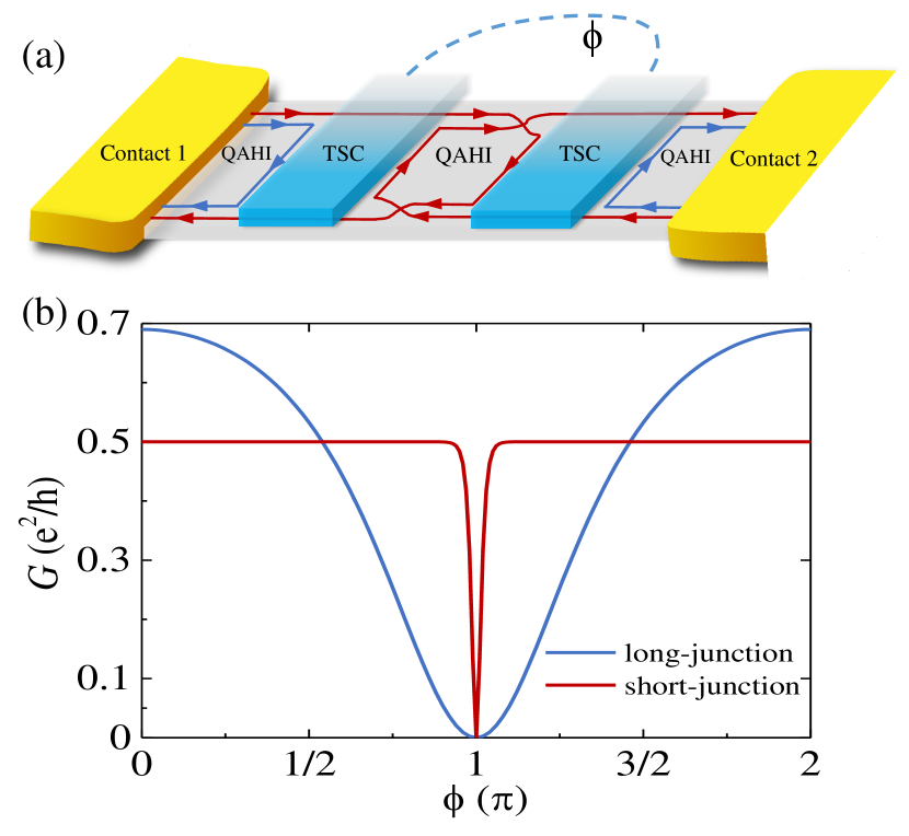
Figure 1: (a) Schematic of a Majorana-Josephson interferometer. A quantum anomalous Hall bar (gray) is in contact with two conventional superconductors (cyan) on its top and two normal metals (yellow) at its ends. The two superconducting contacts are grounded and maintain a tunable phase difference $\phi$. The arrowed lines represent generic scattering of chiral Majorana modes in the interferometer. (b) Typical two-terminal conductance $G$ as a function $\phi$ in a Majorana-Josephson interferometer when the superconducting junction is long (blue line) and short (red line), respectively.

In this paper, we propose a Majorana interferometer with its interference loop generated and controlled by a Josephson junction, as illustrated in Fig. 1(a). The Josephson junction is composed of two topological superconductors (TSCs) induced by conventional superconductors in contact with a QAHI He17sci ; Qi10prb ; ChungSB11prb ; WangJ15prb . Such a Josephson junction effectively polarizes and filters a $\chi$MM in terms of its $U(1)$ degree of freedom associated with the superconducting phase. As a consequence of this novel Majorana valve effect, quantum interference patterns in two-terminal conductance measured with the normal metallic contacts can be observed by tuning the Josephson phase $\phi$, as exemplified in Fig. 1(b). This Majorana-Josephson interferometer (MJI), on the one hand, extends straightforwardly an existing experimental setup He17sci , and hence is expected to be readily accessible. On the other hand, its interference effect demonstrates highly nontrivial Majorana physics, and can be used not only as a smoking-gun signature for the presence of $\chi$MMs, but also potentially in operations of Majorana-based topological quantum computation.

Model for Majorana Josephson interferometer. —The Bogoliubov-de Gennes Hamiltonian that describes the low-energy physics of the MJI sample area is given by Qi10prb ; ChungSB11prb

$$H=\begin{pmatrix}h_{0}(\hat{{\bf k}})-\mu&\Delta(x)\\ \Delta(x)^{*}&h_{0}(-\hat{{\bf k}})+\mu\end{pmatrix},$$ (1)

where $h_{0}(\hat{{\bf k}})=(b\hat{{\bf k}}^{2}-m)\sigma_{z}+v\hat{k}_{x}\sigma_{x}+v\hat{k}_{y}\sigma_{y}$ is the effective Hamiltonian for the underlying QAHI with positive parameters $b$, $m$ and $v$, the Pauli matrices $\sigma_{x,y,z}$ for spin, and two-dimensional wavevector operator $\hat{{\bf k}}\equiv(\hat{k}_{x},\hat{k}_{y})\equiv-i(\partial_{x},\partial_{y})$; $\mu$ is the chemical potential. The proximity-induced pairing potential across the sample is assumed to depend only on $x$ (see Fig. 2): $\Delta(x)=\Delta_{0}$ if $x_{1}<x<x_{2}$; $\Delta_{0}e^{i\phi}$ if $x_{3}<x<x_{4}$; and $0$ otherwise, where $\Delta_{0}$ is taken to be positive, and $\phi$ stands for the Josephson phase. In the Hamiltonian in Eq. (1), we have adopted the Nambu basis which, in real space, reads $\Psi_{{\bf r}}=\left(c_{{\bf r}\uparrow},c_{{\bf r}\downarrow},c_{{\bf r}\downarrow}^{\dagger},-c_{{\bf r}\uparrow}^{\dagger}\right)^{T}$ with $c_{{\bf r}s}$ and $c_{{\bf r}s}^{\dagger}$ the annihilation and creation operators for an electron with spin $s=\uparrow,\downarrow$ at ${\bf r}=(x,y)$, respectively. This Hamiltonian is manifestly particle-hole symmetric: $\mathcal{P}H\mathcal{P}^{-1}=-H$ with the particle-hole operator $\mathcal{P}=\tau_{y}\otimes\sigma_{y}\mathcal{K}$, where $\mathcal{K}$ is the complex conjugate operator, and $\tau_{x,y,z}$ are the Pauli matrices for a Nambu spinor.

The above model defines an MJI if $\Delta_{0}^{2}>m^{2}-\mu^{2}>0$ such that, by labeling the regions with different pairing potentials to be A to E as shown in Fig. 2, the topological invariant $\mathcal{N}=2$ in the bulk of regions A, C and E, and $\mathcal{N}=1$ in the bulk of regions B and D Qi10prb . Throughout this paper, we assume that the relevant energy range, determined by temperature, bias voltages etc., is close enough to zero energy, such that the scattering processes are approximately energy-independent. We also assume that the sizes of regions A and E (B and D) are large compared with the transverse penetration length $\xi_{\mathrm{QAH}}$ ($\xi_{\mathrm{TSC}}$) of the QAHI (TSC) edge modes, such that the scattering channels as depicted in Fig. 2 are well defined. We distinguish, however, two limits in terms of the length of region C, $l_{C}\equiv x_{3}-x_{2}$, which separates the two TSC regions: the long-junction limit with $l_{C}\gg\xi_{\mathrm{QAH}}$, and the short-junction limit with $l_{C}\ll\xi_{\mathrm{QAH}}$.

Before we analyze the transport behaviors of the MJI, it is useful to gain insight from the solutions of the $\chi$MMs, denoted by $\Psi_{B,D}$ in the TSC regions B and D, respectively (see Sec. I in Ref. Note-on-SM ). At $E=0$, both solutions satisfy the Majorana condition $\mathcal{P}\Psi_{B,D}=\Psi_{B,D}$. In addition, because the bulk Hamiltonians in regions B and D differ only in the superconducting phase, $\Psi_{B}$ and $\Psi_{D}$ are related by a simple transformation $\Psi_{D}=U(\phi)\Psi_{B}$ with $U(\phi)=\exp({i\frac{\phi}{2}\tau_{z}})\otimes\sigma_{0}$. As $\mathcal{P}$ is an antiunitary operator, it follows immediately that

$$\langle\Psi_{B}|\Psi_{D}\rangle=\langle\Psi_{D}|\Psi_{B}\rangle=\cos\frac{\phi}{2},$$ (2)

which represents a mismatch between the two $\chi$MMs at finite $\phi$. Physically, this implies an inner $U(1)$ degree of freedom associated with the $\chi$MMs Note-on-MP , or Majorana polarization as analogous to the spin polarization of spin-$\frac{1}{2}$ particles. Thus the TSC Josephson junction effectively becomes a Majorana valve, similar to a spin valve Datta90apl ; Dieny91prb ; Zutic04rmp by the same analogy. This Majorana valve leads directly to an interference loop in the MJI, as we proceed to show.

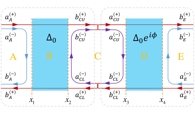
Figure 2: Scattering picture of the chiral Majorana modes in the long-junction limit of a Majorana-Josephson interferometer at $\mu=0$. Regions with different superconducting order parameters are labeled by A through E. The full scattering matrix can be obtained by first analyzing the composite regions ABC and CDE (in gray dashed frames) individually, and then connecting them by taking into account the $\phi$-dependent local basis. Labels for the incoming ($a$’s) and the outgoing ($b$’s) Majorana modes are indicated.

The long-junction limit.— When the two TSC regions are well separated, i.e., when $l_{C}\gg\xi_{\mathrm{QAH}}$, the MJI can be analyzed by first considering the composite ABC region or CDE region individually, and then treating their connection with care. This procedure is particularly physical transparent in the $\mu=0$ case, where the partial Hamiltonian for either region ABC or CDE can be brought to a block-diagonal form by a global unitary transformation Qi10prb ; ChungSB11prb : $U_{p}^{\dagger}H_{p}(\mu=0)U_{p}=h_{p}^{(+)}\oplus h_{p}^{(-)}$ with $p=ABC$ or $CDE$. Here, $h_{p}^{(\pm)}=h_{0}(\hat{{\bf k}})\mp|\Delta(x)|\sigma_{z}$,

$$U_{ABC}=\frac{1}{\sqrt{2}}\begin{pmatrix}\sigma_{0}&\sigma_{0}\\ -\sigma_{z}&\sigma_{z}\end{pmatrix},\quad U_{CDE}=U(\phi)U_{ABC}.$$ (3)

For the sake of clarity, we assume that the partial Hamiltonian with $p=ABC$ ($p=CDE$) is limited to the range $x<\frac{x_{2}+x_{3}}{2}$ ($x>\frac{x_{2}+x_{3}}{2}$). The particle-hole operator in the transformed basis also becomes block-diagonal and is identical for $p=ABC$ and $p=CDE$: $\tilde{\mathcal{P}}\equiv U_{p}^{\dagger}\mathcal{P}U_{p}=-\sigma_{z}\otimes\sigma_{x}\mathcal{K}$, which indicates that each block may allow for $\chi$MM solutions independently. Indeed, the two subspaces corresponding to $h_{p}^{(\pm)}$ each support one $\chi$MM along the QAHI edge, but scattered differently at the QAHI-TSC interfaces (see Fig. 2). This scenario, for $p=ABC$ or $p=CDE$ individually, has been analyzed by Chung et al. ChungSB11prb , and the scattering matrix in the Majorana basis is given by

$$\begin{pmatrix}b_{p,U}^{(+)}\\ b_{p,L}^{(+)}\\ b_{p,U}^{(-)}\\ b_{p,L}^{(-)}\end{pmatrix}=\begin{pmatrix}1&0&0&0\\ 0&1&0&0\\ 0&0&0&-1\\ 0&0&1&0\end{pmatrix}\begin{pmatrix}a_{p,U}^{(+)}\\ a_{p,L}^{(+)}\\ a_{p,U}^{(-)}\\ a_{p,L}^{(-)}\end{pmatrix},$$ (4)

where $a_{p,U/L}^{(+/-)}$ ($b_{p,U/L}^{(+/-)}$) stands for the incoming (outgoing) Majorana current amplitude corresponding to the $h_{p}^{(+/-)}$ block along the upper/lower edge of region $p$. Note that the $-1$ in the above scattering matrix comes from the requirement that the determinant of the full scattering matrix is $+1$ (see Sec. II A in Ref. Note-on-SM ). Hereafter we will abbreviate the labels of these amplitudes according to Fig. 2 without ambiguity.

The key idea of the MJI proposed in this paper is that, despite the trivial appearance of the scattering processes in either the ABC or the CDE region individually, the connection between the two parts is nontrivial as suggested by the Majorana polarization mismatch in Eq. (2). The same mismatch is reflected in Eq. (3) as the different basis used for $p=ABC$ and $p=CDE$ in block-diagonalizing the partial Hamiltonians when $\phi\neq 0$. It follows that the change of basis introduces effective scattering between the $\chi$MMs as (see Sec. II A in Ref. Note-on-SM )

$$\begin{pmatrix}a_{C\beta}^{(+)}\\ a_{C\beta}^{(-)}\end{pmatrix}=\begin{pmatrix}\cos\varphi_{\beta}&\sin\varphi_{\beta}\\ -\sin\varphi_{\beta}&\cos\varphi_{\beta}\end{pmatrix}\begin{pmatrix}b_{C\beta}^{(+)}\\ b_{C\beta}^{(-)}\end{pmatrix},$$ (5)

where $\beta=U,L$ and $\varphi_{U/L}=\pm\phi/2$. Combining this equation and Eq. (4), we obtain the full Majorana scattering matrix connecting the two normal contacts to be

$$\begin{pmatrix}b_{E}^{(+)}\\ b_{A}^{(+)}\\ b_{E}^{(-)}\\ b_{A}^{(-)}\end{pmatrix}=\begin{pmatrix}t&-r&0&0\\ r&t&0&0\\ 0&0&0&-1\\ 0&0&1&0\end{pmatrix}\begin{pmatrix}a_{A}^{(+)}\\ a_{E}^{(+)}\\ a_{A}^{(-)}\\ a_{E}^{(-)}\end{pmatrix},$$ (6)

where $t=\frac{2\cos\frac{\phi}{2}}{1+\cos^{2}\frac{\phi}{2}}$ and $r=\frac{1-\cos^{2}\frac{\phi}{2}}{1+\cos^{2}\frac{\phi}{2}}$. Thus the MJI functions effectively as a Fabry-Perot interferometer for $\chi$MMs LiJ12prb ; LawKT09prl with its transmission and reflection amplitudes tuned by the Josephson phase $\phi$.

More generally, when $\mu\neq 0$, the global transformation that block-diagonalizes either partial Hamiltonian $H_{p}$ is not readily available, such that we need to begin with generic scattering matrices at the QAHI-TSC interfaces. To make progress, we use symmetry analysis and reduction (see Sec. II B in Ref. Note-on-SM ). The strategy here is the same as in Ref. LiJ12prb : By exploiting the particle-hole symmetry and the electronic $U(1)$ gauge degree of freedom, we can reduce a generic scattering matrix to its canonical, yet still general, form which contains only symmetry-compliant and physically relevant parameters. This leads to formally the same scattering matrices as in Eqs. (4-6) except that: first, the Majorana basis here is no longer attached to any (globally) block-diagonalized Hamiltonians; second, $\varphi_{U}$ and $\varphi_{L}$ in general become independent, such that the expressions for $t$ and $r$ in Eq. (6) become $t=({\cos\varphi_{U}+\cos\varphi_{L}})/({1+\cos\varphi_{U}\cos\varphi_{L}})$ and $r=-{\sin\varphi_{U}\sin\varphi_{L}}/({1+\cos\varphi_{U}\cos\varphi_{L}})$. Indeed, by considering two limiting cases, with $\mu=0$ or $\phi=0$, respectively, it is straightforward to deduce $\varphi_{U/L}=\pm\phi/2+k_{F}l_{C}$, where $k_{F}$ is the Fermi wave vector for the QAHI edge mode in region C. For the Hamiltonian in Eq. (1), $k_{F}=\mu/v$. Physically, this means that the propagation of a QAHI edge mode at a finite momentum effectively introduces precession of Majorana polarization to the composing $\chi$MMs Note-on-MP . Finally, we obtain the Majorana transmission and reflection amplitudes,

$$t=\frac{2\cos(k_{F}l_{C})\cos({\phi}/{2})}{\cos^{2}(k_{F}l_{C})+\cos^{2}({\phi}/{2})},\;r=\frac{\cos^{2}(k_{F}l_{C})-\cos^{2}({\phi}/{2})}{\cos^{2}(k_{F}l_{C})+\cos^{2}({\phi}/{2})},$$ (7)

which are to be substituted into Eq. (6).

By using the scattering theory developed for $\chi$MM interferometry in Ref. LiJ12prb , we further write down the average current and the zero-frequency zero-temperature noise (shot noise) power in the two normal contacts,

$$I_{n}=\frac{e^{2}}{h}(1-r)V_{n},\qquad(n=1,2),$$ (8)

$$I_{s}=-(I_{1}+I_{2})=-\frac{e^{2}}{h}(1-r)(V_{1}+V_{2}),$$ (9)

$$P_{a}=\frac{e^{3}}{h}\frac{t^{2}}{2}\max(|V_{1}|,|V_{2}|),$$ (10)

$$P_{c}=\frac{e^{3}}{h}\frac{t^{2}}{2}\text{sgn}(V_{1}V_{2})\min(|V_{1}|,|V_{2}|),$$ (11)

where $V_{n}$ is the bias voltage applied on contact $n=1,2$; $I_{n}\equiv\langle\hat{I}_{n}\rangle$ is the time-averaged current through normal contact $n$; $I_{s}$ is the time-averaged total current through the superconducting contacts to the ground; $P_{a}\equiv P_{11}=P_{22}$ and $P_{c}\equiv P_{12}=P_{21}$ are the auto-correlator and the cross-correlator, respectively; $P_{nn^{\prime}}\equiv\int_{-\infty}^{\infty}dt\,\frac{1}{2}\langle\{\hat{I}_{n}(t)-{I}_{n},\,\hat{I}_{n^{\prime}}(0)-{I}_{n^{\prime}}\}\rangle$, with $\{$,$\}$ standing for the anti-commutator, is the zero-frequency current correlation function (noise power) between normal contact $n$ and $n^{\prime}$ Buttiker92prb ; Blanter00pr . Several remarks are in order. First, the average current $I_{n}$ in contact $n$ appears only depending on $r$ and $V_{n}$ on the same contact $n$. This is a common feature of $\chi$MM interferometers resulting from the fact that electric current can always be interpreted as interference between two $\chi$MMs Note-on-CMM – only Majoranas sourced from the same contact can maintain quantum phase coherence in single-particle scattering processes, and therefore contribute to a nonvanishing average current. Second, the current correlation functions, in contrast to the average current, generally depend on $t$, and the bias voltages on both normal contacts. In particular, the current cross-correlator $P_{c}$ is contributed solely by the exchange of two Majoranas sourced from different contacts in the form of identical particles LiJ12prb . Third, if measurements are made by setting $I_{s}=0$, then the bias voltages must satisfy $V_{1}=-V_{2}$. In this case, we denote $V_{0}=V_{1}-V_{2}=2V_{1}$, and $I_{0}=I_{1}=-I_{2}$. From Eq. (8) we immediately obtain the two-terminal conductance, $G\equiv I_{0}/V_{0}$, to be

$$G_{\textrm{long}}=\frac{e^{2}}{h}\frac{\cos^{2}({\phi}/{2})}{\cos^{2}(k_{F}l_{C})+\cos^{2}({\phi}/{2})},$$ (12)

Clearly, $G_{\textrm{long}}$ oscillates with both $\phi$ and $k_{F}l_{C}$ as a consequence of the interference effect.

The short-junction limit.—When the separation $l_{C}$ between regions B and D becomes comparable to or less than $\xi_{\mathrm{QAH}}$, the otherwise well-separated $\chi$MMs along the B-C and the C-D interfaces strongly hybridize to become Andreev bound states. The spectrum of these Andreev bound states is generally gapped unless the Josephson phase $\phi\mod 2\pi=\pi$ FuL08prl ; FuL09prb . In this case, it is necessary to take into account the finite width $W$ of any realistic sample, and hence the finite tunneling rate of $\chi$MMs between the upper and the lower edges through the interface, especially when the gap of the Andreev bound state spectrum approaches 0. In the following, we demonstrate the generic behavior of the MJI in the short-junction limit by assuming $\mu=0$ and $l_{C}=0$ for simplicity.

At the interface between the two TSCs (regions B and D with $l_{C}=0$), the Andreev bound state dispersion can be solved at low energy to be (see Sec. III A in Ref. Note-on-SM )

$$E_{\text{Andreev}}\simeq\pm\sqrt{(vk_{y})^{2}+(\varepsilon\delta\phi)^{2}},$$ (13)

where $\varepsilon=(\Delta_{0}^{2}-m^{2})/(2\Delta_{0})$ and $\delta\phi\equiv(\phi-\pi)\mod 2\pi$. This indicates the gap along the interface varies as $|\varepsilon\delta\phi|$ when $\delta\phi$ is small, and the penetration depth along $\hat{y}$ of the evanescent states at $E=0$ is $\xi_{\phi}=v/|\varepsilon\delta\phi|$. When $\xi_{\phi}\gtrsim W$, the tunneling of $\chi$MMs between the upper and the lower edge of the sample along the interface becomes significant Wieder14 . Such a tunneling problem can be explicitly solved in the form of an effective model for the $\chi$MMs (see Sec. III B in Ref. Note-on-SM ), which leads to the scattering relation (cf. Eq. (6))

$$\begin{pmatrix}b_{E}^{(+)}\\ b_{A}^{(+)}\end{pmatrix}=\begin{pmatrix}\tanh(W/\xi_{\phi})&-\text{sech}(W/\xi_{\phi})\\ \text{sech}(W/\xi_{\phi})&\tanh(W/\xi_{\phi})\end{pmatrix}\begin{pmatrix}a_{A}^{(+)}\\ a_{E}^{(+)}\end{pmatrix}.$$ (14)

Subsequently we obtain the average current and the current correlators by substituting $t=\tanh(W/\xi_{\phi})$ and $r=\text{sech}(W/\xi_{\phi})$ into Eqs. (8-11). In particular, by setting $I_{s}=0$, the two-terminal conductance becomes

$$G_{\textrm{short}}\simeq\frac{e^{2}}{h}\frac{1-\text{sech}(\varepsilon W\delta\phi/v)}{2},$$ (15)

which vanishes when $\delta\phi=0$ and saturates to $e^{2}/2h$ when $\delta\phi\gg v/\varepsilon W$. Incidentally, we note that in the short-junction limit of the MJI, the topological property of region C becomes irrelevant as long as the interface $\chi$MMs couple strongly to form Andreev bound states.

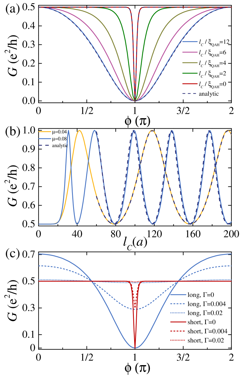
Figure 3: (a) Two-terminal conductance $G$ as a function of $\phi$ for different junction length $l_{C}$ with the chemical potential $\mu=0$. The solid lines are numerical results, whereas the dashed lines are analytical results for the long-junction and the short-junction limits, respectively. (b) $G$ as a function of $l_{C}$ with different $\mu$ at $\phi=0$. The solid lines are numerical results, whereas the dashed lines are analytical results for the long-junction limit plotted from $l_{C}=60a$. (c) $G$ as a function of $\phi$ for different inverse quasiparticle life time $\Gamma$ with $\mu=0.04$, in the long-junction (blue line, $l_{C}=100a$) and the short-junction (red line) limits, respectively. All plots here share the following parameters: $W=200a$, $x_{2}-x_{1}=x_{4}-x_{3}=100a$, $b=v=1$, $\Delta_{0}=3m=0.3$. With these parameters we estimate $\xi_{\mathrm{QAH}}/a\approx v/(2m)=5$.

Numerical simulations.— Up to now we have analyzed two limits of the MJI to demonstrate its generic transport behavior, as highlighted in Fig. 1(b). In order to extend our results to general settings beyond the analytically tractable ones, we perform numerical simulations based on the discretized version (with the lattice constant $a=1$) of the Hamiltonian in Eq. (1), by using the Landauer-B$\ddot{\mathrm{u}}$ttiker formalism Buttiker92prb ; Landauer70pm ; Buttiker86prl ; Fisher81prb ; Dattabook adapted to superconducting systems Anantram96prb . First of all, we verify our preceding analytical results in Eqs. (12) and (15)). The dependence of the numerically calculated two-terminal conductance $G$ (see Sec. IV A in Ref. Note-on-SM ) on the Josephson phase $\phi$ and the junction length $l_{C}$ is shown in Figs. 3(a) and (b), respectively. We find very good agreement between our numerical and analytical results in both the long-junction and the short-junction limits. Next, we examine the effect of inelastic scattering in the form of a finite quasiparticle life time Ji18prl ; HuangY18prb , signified by $1/\Gamma$ (see Sec. IV C in Ref. Note-on-SM ). Evidently shown in Fig. 3(c), the interference pattern weakens with increasing $\Gamma$, and disappears when $G$ becomes a constant $e^{2}/2h$ at large enough $\Gamma$ Ji18prl ; HuangY18prb .

Discussion.—One obvious advantage of the MJI is that its interference pattern is a direct manifestation of phase coherent $\chi$MM transport, and hence can be used as a smoking-gun signature for the presence of $\chi$MMs in the setup. This will solve the current controversy over the origin of the half-quantized conductance plateau in the experiment reported in Ref. He17sci – the trivial mechanisms such as those proposed in Refs. Ji18prl ; HuangY18prb generally rely on substantial electron inelastic scattering especially around the half-quantized plateau region, which necessarily destroys the interference pattern. As such, the MJI can also be used as a tool to measure the decoherence rate of the $\chi$MMs caused by various environmental noises. Here, we stress that the physics of the interference effect in an MJI is intrinsically different from that of the well-established dc Josephson effect: The former concerns the nonequilibrium current carried by the $\chi$MMs and measured at the normal metallic contacts; the latter concerns the equilibrium supercurrent through the superconducting contacts that is not necessarily associated with any $\chi$MMs olund_current-phase_2012 ; snelder_andreev_2013 ; chen_emergent_2018 . More importantly, the MJI may further offer an effective platform for the braiding of chiral Majorana fermions LianB17arXiv , or even the manipulation of Majorana qubits that can be defined upon the Majorana zero modes induced in the vortices in the TSC regions Beenakker18arXiv . An in-depth investigation in this direction will be the subject of our future work.

- (1) N. Read and D. Green, Phys. Rev. B 61, 10267 (2000).
- (2) A. Y. Kitaev, Phys. Usp. 44, 131 (2001).
- (3) L. Fu and C. L. Kane, Phys. Rev. Lett. 100, 096407 (2008).
- (4) Y. Oreg, G. Refael, and F. von Oppen, Phys. Rev. Lett. 105, 177002 (2010).
- (5) R. M. Lutchyn, J. D. Sau, and S. Das Sarma, Phys. Rev. Lett. 105, 077001 (2010).
- (6) F. Wilczek, Nat. Phys. 5, 614 (2009).
- (7) J. Alicea, Rep. Prog. Phys. 75, 076501 (2012).
- (8) C. Beenakker, Annu. Rev. Condens. Matter Phys. 4, 113 (2013).
- (9) S. R. Elliott and M. Franz, Rev. Mod. Phys. 87, 137 (2015).
- (10) M. Sato and Y. Ando, Rep. Prog. Phys. 80, 076501 (2017).
- (11) S.-Q. Shen, Topological Insulators: Dirac Equation in Condensed Matter, 2nd ed. (Springer, Singapore, 2017).
- (12) A. Kitaev, Ann. Phys. 303, 2 (2003).
- (13) C. Nayak, S. H. Simon, A. Stern, M. Freedman, and S. Das Sarma, Rev. Mod. Phys. 80, 1083 (2008).
- (14) J. Alicea, Y. Oreg, G. Refael, F. von Oppen, and M. P. A. Fisher, Nat. Phys. 7, 412 (2011).
- (15) A. Stern and N. H. Lindner, Science 339, 1179 (2013).
- (16) S. D. Sarma, M. Freedman, and C. Nayak, npj Quantum Inf. 1, 15001 (2015).
- (17) T. Karzig, C. Knapp, R. M. Lutchyn, P. Bonderson, M. B. Hastings, C. Nayak, J. Alicea, K. Flensberg, S. Plugge, Y. Oreg, C. M. Marcus, and M. H. Freedman, Phys. Rev. B 95, 235305 (2017).
- (18) T. E. O’Brien, P. Rozek, and A. R. Akhmerov, Phys. Rev. Lett. 120, 220504 (2018).
- (19) D. Litinski and F. von Oppen, Phys. Rev. B 97, 205404 (2018).
- (20) V. Mourik, K. Zuo, S. M. Frolov, S. R. Plissard, E. P. A. M. Bakkers, and L. P. Kouwenhoven, Science 336, 1003 (2012).
- (21) J. R. Williams, A. J. Bestwick, P. Gallagher, S. S. Hong, Y. Cui, A. S. Bleich, J. G. Analytis, I. R. Fisher, and D. Goldhaber-Gordon, Phys. Rev. Lett. 109, 056803 (2012).
- (22) M. T. Deng, C. L. Yu, G. Y. Huang, M. Larsson, P. Caroff, and H. Q. Xu, Nano Lett. 12, 6414 (2012).
- (23) A. Das, Y. Ronen, Y. Most, Y. Oreg, M. Heiblum, and H. Shtrikman, Nat. Phys. 8, 887 (2012).
- (24) S. Nadj-Perge, I. K. Drozdov, J. Li, H. Chen, S. Jeon, J. Seo, A. H. MacDonald, B. A. Bernevig, and A. Yazdani, Science 346, 602 (2014).
- (25) J. P. Xu, M. X. Wang, Z. L. Liu, J. F. Ge, X. Yang, C. Liu, Z. A. Xu, D. Guan, C. L. Gao, D. Qian, Y. Liu, Q. H. Wang, F. C. Zhang, Q. K. Xue, and J.-F. Jia, Phys. Rev. Lett. 114, 017001 (2015).
- (26) S. Jeon, Y. Xie, J. Li, Z. Wang, B. A. Bernevig, and A. Yazdani, Science 358, 772 (2017).
- (27) Q. L. He, L. Pan, A. L. Stern, E. C. Burks, X. Che, G. Yin, J. Wang, B. Lian, Q. Zhou, E. S. Choi, K. Mu- rata, X. Kou, Z. Chen, T. Nie, Q. Shao, Y. Fan, S.-C. Zhang, K. Liu, J. Xia, and K. L. Wang, Science 357, 294 (2017).
- (28) P. Zhang, K. Yaji, T. Hashimoto, Y. Ota, T. Kondo, K. Okazaki, Z. Wang, J. Wen, G. D. Gu, H. Ding, and S. Shin, Science 360, 182 (2018).
- (29) H. Zhang, C.-X. Liu, S. Gazibegovic, D. Xu, J. A. Logan, G. Wang, N. van Loo, J. D. S. Bommer, M. W. A. de Moor, D. Car, R. L. M. Op het Veld, P. J. van Veldhoven, S. Koelling, M. A. Verheijen, M. Pendharkar, D. J. Pennachio, B. Shojaei, J. S. Lee, C. J. Palmstrom, E. P. A. M. Bakkers, S. D. Sarma, and L. P. Kouwenhoven, Nature (London) 556, 74 (2018).
- (30) B. A. Bernevig and T. L. Hughes, Topological insulators and topological superconductors (Princeton University Press, Princeton, NJ, 2013).
- (31) G. Moore and N. Read, Nucl. Phys. B 360, 362 (1991).
- (32) X. G. Wen, Phys. Rev. Lett. 66, 802 (1991).
- (33) D. A. Ivanov, Phys. Rev. Lett. 86, 268 (2001).
- (34) A. Stern, Nature 464, 187 (2010).
- (35) S. Das Sarma, M. Freedman, and C. Nayak, Phys. Rev. Lett. 94, 166802 (2005).
- (36) P. Bonderson, K. Shtengel, and J. K. Slingerland, Phys. Rev. Lett. 97, 016401 (2006).
- (37) D. E. Feldman, and A. Kitaev, Phys. Rev. Lett. 97, 186803 (2006).
- (38) W. Bishara, P. Bonderson, C. Nayak, K. Shtengel, and J. K. Slingerland, Phys. Rev. B 80, 155303 (2009).
- (39) K. T. Law, P. A. Lee, and T. K. Ng, Phys. Rev. Lett. 103, 237001 (2009).
- (40) L. Fu, and C. L. Kane, Phys. Rev. Lett. 102, 216403 (2009).
- (41) A. R. Akhmerov, Johan Nilsson, and C. W. J. Beenakker, Phys. Rev. Lett. 102, 216404 (2009).
- (42) G. Strbi, W. Belzig, M.-S. Choi, and C. Bruder, Phys. Rev. Lett. 107, 136403 (2011).
- (43) J. Li, G. Fleury, and M. Bttiker, Phys. Rev. B 85, 125440 (2012).
- (44) X. L. Qi, T. L. Hughes, and S. C. Zhang, Phys. Rev. B 82, 184516 (2010).
- (45) S. B. Chung, X. L. Qi, J. Maciejko, and S. C. Zhang, Phys. Rev. B 83, 100512 (2011).
- (46) J. Wang, Q. Zhou, B. Lian, and S. C. Zhang, Phys. Rev. B 92, 064520 (2015).
- (47) R. Yu, W. Zhang, H. J. Zhang, S. C. Zhang, X. Dai, and Z. Fang, Science 329, 61 (2010).
- (48) C. Z. Chang, J. Zhang, X. Feng, J. Shen, Z. Zhang, M. Guo, K. Li, Y. Ou, P. Wei, L. L. Wang, Z. Q. Ji, Y. Feng, S. Ji, X. Chen, J. Jia, X. Dai, Z. Fang, S. C. Zhang, K. He, Y. Wang, L. Lu, X. C. Ma, and Q. K. Xue, Science 340, 167 (2013).
- (49) H. Z. Lu, A. Zhao, and S. Q. Shen, Phys. Rev. Lett. 111, 146802 (2013).
- (50) W. Ji and X. G. Wen, Phys. Rev. Lett. 120, 107002 (2018).
- (51) Y. Huang, F. Setiawan, and J. D. Sau, Phys. Rev. B 97, 100501 (2018).
- (52) See Supplemental Materials at [URL XXX] for details, which includes Refs. LiJ12prb ; ZhangYT17prb ; Buttiker86prb ; JiangH09prl .
- (53) The origin of Majorana polarization is transparent and is associated with the electronic degree of freedom in defining Majorana modes: and .
- (54) S. Datta and B. Das, Appl. Phys. Lett. 56, 665 (1990).
- (55) B. Dieny, V. S. Speriosu, S. S. P. Parkin, B. A. Gurney, D. R. Wilhoit, and D. Mauri, Phys. Rev. B 43, 1297 (1991).
- (56) I. utic, J. Fabian, and S. Das Sarma, Rev. Mod. Phys. 76, 323 (2004).
- (57) M. Bttiker, Phys. Rev. B 46, 12485 (1992).
- (58) Y. M. Blanter and M. Bttiker, Phys. Rep. 336, 1 (2000).
- (59) As an intuitive way to see the interpretation of electric current as interference between two MMs, we simply notice that the electron number operator can be expressed in terms of the multiplication of two Majorana operators: if and , then .
- (60) L. Fu and C. L. Kane, Phys. Rev. B 79, 161408 (2009).
- (61) B. J. Wieder, F. Zhang, and C. L. Kane, Phys. Rev. B 89, 075106 (2014).
- (62) R. Landauer, Philos. Mag. 21, 863(1970).
- (63) M. Bttiker, Phys. Rev. Lett. 57, 1761 (1986).
- (64) D. S. Fisher and P. A. Lee, Phys. Rev. B 23, 6851 (1981).
- (65) S. Datta, Electronic Transport in Mesoscopic Systems (Cambridge University Press, Cambridge, U.K., 1995).
- (66) M. P. Anantram and S. Datta, Phys. Rev. B 53, 16390 (1996).
- (67) C. T. Olund and E. Zhao, Phys. Rev. B 86, 214515 (2012).
- (68) M. Snelder, M. Veldhorst, A. A. Golubov, and A. Brinkman, Phys. Rev. B 87, 104507 (2013).
- (69) C.-Z. Chen, J. J. He, D.-H. Xu, and K. T. Law, Phys. Rev. B 98, 165439 (2018).
- (70) B. Lian, X.-Q. Sun, A. Vaezi, X.-L. Qi, and S.-C. Zhang, Proc. Natl. Acad. Sci. USA 115, 10938 (2018).
- (71) C. W. J. Beenakker, P. Baireuther, Y. Herasymenko, I. Adagideli, L. Wang, and A. R. Akhmerov, arXiv:1809.09050 (2018).
- (72) Y.-T. Zhang, Z. Hou, X. C. Xie, and Q.-F. Sun, Phys. Rev. B 95, 245433 (2017).
- (73) M. Bttiker, Phys. Rev. B 33, 3020 (1986).
- (74) H. Jiang, S. Cheng, Q.-F. Sun, and X. C. Xie, Phys. Rev. Lett. 103, 036803 (2009).