Galerkin Approximation of Dynamical Quantities using Trajectory Data

Abstract

Understanding chemical mechanisms requires estimating dynamical statistics such as expected hitting times, reaction rates, and committors. Here, we present a general framework for calculating these dynamical quantities by approximating boundary value problems using dynamical operators with a Galerkin expansion. A specific choice of basis set in the expansion corresponds to estimation of dynamical quantities using a Markov state model. More generally, the boundary conditions impose restrictions on the choice of basis sets. We demonstrate how an alternative basis can be constructed using ideas from diffusion maps. In our numerical experiments, this basis gives results of comparable or better accuracy to Markov state models. Additionally, we show that delay embedding can reduce the information lost when projecting the system’s dynamics for model construction; this improves estimates of dynamical statistics considerably over the standard practice of increasing the lag time.

I Introduction

Molecular dynamics simulations allow chemical mechanisms to be studied with atomistic detail. By averaging over trajectories, one can estimate dynamical statistics such as mean first-passage times or committors. These quantities are integral to chemical rate theories.Kramers (1940); Hänggi, Talkner, and Borkovec (1990); Vanden-Eijnden (2006) However, events of interest often occur on timescales several orders of magnitude longer than the timescales of microscopic fluctuations. In such cases, collecting chemical-kinetic statistics by integrating the system’s equations of motion and directly computing averages (sample means) requires prohibitively large amounts of computational resources.

The traditional way to address this separation in timescales was through theories of activated processes.Hänggi, Talkner, and Borkovec (1990); Berezhkovskii et al. (2014) By assuming that the kinetics are dominated by passage through a single transition state, researchers were able to obtain approximate analytical forms for reaction rates and related quantities. These expressions can be connected with microscopic simulations by evaluating contributing statistics such as the potential of mean force and the diffusion tensor.Ma, Nag, and Dinner (2006); Ovchinnikov, Nam, and Karplus (2016); Ghysels et al. (2017) However, many processes involve multiple reaction pathways, such as the folding of larger proteins Dinner and Karplus (1999); Dinner et al. (2000). In these cases it may not be possible in practice, or even in principle, to represent the system in a way that the assumptions underlying theories of activated processes are reasonable.

More recently, rates and other dynamical statistics have been estimated using transition path sampling algorithms. These focus sampling only on the pathways connecting metastable states.Dellago et al. (1998); Bolhuis et al. (2002) While this can be done efficiently if these pathways are short, if they are long and include multiple intermediates the sampling task becomes difficult.Grünwald, Dellago, and Geissler (2008); Gingrich and Geissler (2015) Another approach is to use splitting schemes, which aim to efficiently direct sampling by intelligently splitting and reweighting short trajectory segments.Huber and Kim (1996); van Erp, Moroni, and Bolhuis (2003); Faradjian and Elber (2004); Allen, Frenkel, and ten Wolde (2006); Warmflash, Bhimalapuram, and Dinner (2007); Vanden-Eijnden and Venturoli (2009); Dickson, Warmflash, and Dinner (2009); Guttenberg, Dinner, and Weare (2012); Bello-Rivas and Elber (2015); Dinner et al. (2018) Some of these methods can yield results that are exact up to statistical precision, with minimal assumptions about the dynamics Warmflash, Bhimalapuram, and Dinner (2007); Vanden-Eijnden and Venturoli (2009); Dickson, Warmflash, and Dinner (2009); Guttenberg, Dinner, and Weare (2012); Bello-Rivas and Elber (2015); Dinner et al. (2018). However, the efficiency of these schemes is generally dependent on a reasonable choice of low-dimensional collective variable (CV) space: a projection of the system’s phase space. Not only can this choice be nonobvious, it can be statistic specific. Moreover, starting and stopping the molecular dynamics many times based on the values of the CVs may be impractical depending on the implementation of the molecular dynamics engine and the overhead associated with computational communication.

A third approach is the construction of Markov state models (MSMs).Schütte et al. (1999); Swope, Pitera, and Suits (2004); Pande, Beauchamp, and Bowman (2010) Here, the dynamics of the system are modeled as a discrete-state Markov chain with state-to-state transition probabilities estimated from previously sampled data. Projecting the dynamics onto a finite-dimensional model introduces a systematic bias, although this bias goes to zero in the correct limit of infinitely many states.Sarich, Noé, and Schütte (2010) While MSMs were initially developed as a technique for approximating the slowest eigenmodes of a system’s dynamics,Schütte et al. (1999) MSMs can also be used to calculate dynamical statistics for the study of kinetics.Noé and Fischer (2008); Noé and Prinz (2014); Keller, Aleksic, and Donati (2019) Since MSM construction only requires time pairs separated by a single lag time, one has more freedom in how one generates the molecular dynamics data. In particular, if the lag time is sufficiently short, MSMs can be used to estimate rates even in the absence of full reactive trajectories. Constructing an efficient MSM requires projection onto CVs, and the systematic error in the resulting estimates can depend strongly on how they are defined. However, the CV space can generally be higher dimensional since it is only used to define Markov states.

It has been shown that calculating the system’s eigenmodes with MSMs can be generalized to a basis expansion of the eigenmodes using an arbitrary basis set.Weber (2006); Sarich, Noé, and Schütte (2010); Noé and Nüske (2013) In this paper, we show that a similar generalization is possible for other dynamical statistics. Rather than solving eigenproblems, these quantities solve linear boundary value problems. This raises additional challenges: not only do the solutions obey specific boundary conditions, the resulting approximations are sensitive to the choice of lag time. We provide numerical schemes to address these difficulties.

We organize our work as follows. In Section II we give background on the transition operator and review both MSMs and more general schemes for data-driven analysis of the spectrum of dynamical operators. We then continue our review with the connection between operator equations and chemical kinetics in Section III. In Section IV we present our formalism. We discuss the choice of basis set in Section V and introduce a new algorithm for constructing basis sets that obey the boundary conditions our formalism requires. In Section VI we show that delay embedding can recover information lost in projecting the system’s dynamics onto a few degrees of freedom, negating the need for increasing the scheme’s lag time to enforce Markovianity. We then demonstrate our algorithm on a collection of long trajectories of the Fip35 WW domain dataset in Section VII, and conclude in Section VIII.

II Background

Many key quantities in chemical kinetics can be expressed through solutions to linear operator equations. Key to this formalism is the transition operator. We begin by assuming that the system’s dynamics are given by a Markov process $\xi^{(t)}$ that is time-homogeneous, i.e. that the dynamics are time-independent. We do not put any restrictions on the nature of the system’s state space. For example, if $\xi$ is a diffusion process, the state space could be the space of real coordinates, $\mathbb{R}^{n}$. Similarly, for a finite-state Markov chain, it would be a finite set of configurations. We also do not assume that the dynamics are reversible or that the system is in a stationary state unless specifically noted.

The transition operator at a lag time of $s$ is defined as

$$\mathcal{K}_{s}f(x)=\mathrm{\mathbf{E}}\left[f\left(\xi^{(s)}\right)|\xi^{(0)}=x\right],$$ (1)

where $f$ is a function on the state space, and $\mathrm{\mathbf{E}}$ denotes expectation. Note that due to time-homogeneity, we could just as easily have defined the transition operator with the time pair $\left(\xi^{(t)},\xi^{(t+s)}\right)$ in place of $\left(\xi^{(0)},\xi^{(s)}\right)$. Depending on the context in question, $\mathcal{K}_{s}$ may also be referred to as the Markov or Koopman operator.Eisner et al. (2015); Klus et al. (2018) We use the term transition operator as it is well established in the mathematical literature and stresses the notion that $\mathcal{K}_{s}$ is the generalization of the transition matrix for finite-state Markov processes. For instance, the requirement that the rows of a transition matrix sum to one generalizes to

$$\mathcal{K}_{s}1=\mathrm{\mathbf{E}}\left[1|\xi^{(0)}=x\right]=1.$$ (2)

Studying the transition operator provides, in principle, a route to analyzing the system’s dynamics. Unfortunately $\mathcal{K}_{s}$ is often either unknown or too complicated to be studied directly. This has motivated research into data-driven approaches that instead treat $\mathcal{K}_{s}$ indirectly by analyzing sampled trajectories.

II.1 Markov State Modeling

One approach to studying chemical dynamics through the transition operator is the construction of Markov state models.Schütte et al. (1999); Swope, Pitera, and Suits (2004); Pande, Beauchamp, and Bowman (2010) In this technique one constructs a Markov chain on a finite state space to model the true dynamics of the system. The transition matrix of this Markov chain is then taken as a model for the true transition operator.

To construct an MSM from trajectory data, we partition the system’s state space into $M$ nonoverlapping sets. We refer to these sets as Markov states and denote them as $S_{i}$. Now, let $\mu$ be an arbitrary probability measure. If the system is initially distributed according to $\mu$, the probability of transitioning from a set $S_{i}$ to $S_{j}$ after a time $s$ is given by

$$P_{ij}=\frac{\int\mathds{1}_{S_{i}}(x)\mathcal{K}_{s}\mathds{1}_{S_{j}}(x)\mu(dx)}{\int\mathds{1}_{S_{i}}(x)\mu(dx)},$$ (3)

where $\mathds{1}_{S_{i}}$ is the indicator function

$$\mathds{1}_{S_{i}}(x)=\begin{cases}1\text{ for }x\text{ in }S_{i}\\ 0\text{ otherwise.}\end{cases}$$ (4)

Here $\int f(x)\mu(dx)$ is the expectation with respect to the probability measure $\mu$.Billingsley (2008) When $\mu$ has a probability density function this integral is the same as the integral against the density, and in a finite state space it would be a weighted average over states. This formalism lets us treat both continuous and discrete state spaces with one notation.

Because the sets $S_{i}$ partition the state space, a simple calculation shows that the elements in each row of $P_{ij}$ sum to one. $P_{ij}$ therefore defines a transition matrix for a finite-state Markov process where state $i$ corresponds to the set $S_{i}$. The dynamics of this process are a model for the true dynamics, and $P_{ij}$ is a model for the transition operator.

To build this model, we construct an estimate of $P_{ij}$ from sampled data. A simple approach is to collect a dataset consisting of $N$ time pairs, $(X_{n},Y_{n})$. Here the initial point $X_{n}$ is drawn from $\mu$, and $Y_{n}$ is collected by starting at $X_{n}$ and propagating the dynamics for time $s$. Note that since the choice of $\mu$ in (3) is relatively arbitrary, it can be defined implicitly through the sampling procedure. For instance, one can construct a dataset by extracting all pairs of points separated by the lag time $s$ from a collection of trajectories; since we have assumed the dynamics are time-homogeneous, the actual physical time at which $X_{n}$ was collected does not matter. We then define $\mu$ to be the measure from which our initial points $X_{n}^{(0)}$ were sampled. With this dataset, $P_{ij}$ is now approximated as

$$\bar{P}_{ij}=\frac{\sum_{n=1}^{N}\mathds{1}_{S_{j}}\left(Y_{n}\right)\mathds{1}_{S_{i}}\left(X_{n}\right)}{\sum_{n=1}^{N}\mathds{1}_{S_{i}}\left(X_{n}\right)}$$ (5)

Like $P_{ij}$, (5) defines a valid transition matrix. This is not the only approach for constructing estimates of $P_{ij}$. One commonly used approach modifies this procedure to ensure that $\bar{P}_{ij}$ gives reversible dynamics. In this approach, one adds a self-consistent iteration that seeks to find the reversible transition matrix with the maximum likelihood given the data.Bowman et al. (2009); Prinz et al. (2011)

The MSM approach has many attractive features. Conceptually, an MSM gives a reduced model of the dynamics which helps the practitioner gain intuition. MSMs can also be used to calculate a wide class of dynamical quantities, including committors, reaction rates, and expected hitting times.Noé and Fischer (2008); Noé and Prinz (2014); Keller, Aleksic, and Donati (2019) Importantly, as constructing MSMs only requires datapoints separated by a short lag time, these long-time dynamical quantities can be evaluated using a collection of short trajectories.Noé et al. (2009) In this paper, we focus exclusively on the latter application and consider MSMs as a technique for calculating the dynamical quantities required in rate theories.

The accuracy with which $P_{ij}$ approximates $\mathcal{K}_{s}$ depends strongly on the choice of the sets $S_{i}$, and choosing good sets is a nontrivial problem in high-dimensional state spaces.Schwantes and Pande (2013); Pérez-Hernández et al. (2013); Schwantes, McGibbon, and Pande (2014); Schütte and Sarich (2015); Shukla et al. (2015) To address this issue, states are generally constructed by projecting the system’s state space onto a CV space. Sets are then defined by either gridding the CV space or clustering sampled configurations based on the values of their CVs. Unfortunately, when gridding, the number of states grows exponentially with the dimension of the CV space. This is not necessarily the case for partitioning schemes based on data clustering and recent work in this direction appears promising. Prinz et al. (2011); Berezovska, Prada-Gracia, and Rao (2013); Sheong et al. (2014); Li and Dong (2016); Husic and Pande (2017); Husic et al. (2018) However, effectively clustering high-dimensional data is a nontrivial problem,Steinbach, Ertöz, and Kumar (2004); Kriegel, Kröger, and Zimek (2009) and constructing an MSM that accurately reflects the dynamics may still require knowledge of a good, relatively low-dimensional CV space. Schwantes and Pande (2013); Pérez-Hernández et al. (2013); Scherer et al. (2015)

II.2 Data-driven Solutions to Eigenfunctions of Dynamical Operators

A related approach to characterizing chemical systems is to estimate the eigenfunctions and eigenvalues of operators associated with the system’s dynamics from sampled data.Klus et al. (2018) These separate the dynamics by timescale: eigenfunctions with larger eigenvalues correlate with the system’s slower degrees of freedom. These eigenfunctions and eigenvalues can often be approximated from trajectory data, even when the transition operator is unknown. Multiple schemes that attempt this have been proposed, often independently, in different fields.Molgedey and Schuster (1994); Takano and Miyashita (1995); Hirao, Koseki, and Takano (1997); Schütte et al. (1999, 2011); Weber (2006); Noé and Nüske (2013); Giannakis, Slawinska, and Zhao (2015); Giannakis (2017); Williams, Kevrekidis, and Rowley (2015) We will refer to the family of these techniques using the umbrella term Dynamical Operator Eigenfunction Analysis (DOEA) for brevity and convenience. Below, we summarize a simple DOEA scheme for the transition operator for the reader’s convenience, largely following work in reference Hirao, Koseki, and Takano, 1997. Other schemes exist and we refer the reader to reference Klus et al., 2018 for further reading.

Here, we consider the solution to the eigenproblem

$$\mathcal{K}_{s}\psi_{l}(x)=\lambda_{l}\psi_{l}(x).$$ (6)

We approximate $\psi_{l}$ as a sum of basis functions $\phi_{j}$ with unknown coefficients $a_{j}$,

$$\psi_{l}(x)=\sum_{j=1}^{M}a_{j}\phi_{j}(x).$$ (7)

This is an example of Galerkin approximation of (6), Schütte et al. (1999) a formalism we cover more closely in Section IV. We now assume our data takes the form discussed in Section II.1. Substituting the basis expansion into (6), multiplying by $\phi_{i}(x)$, and taking the expectation against $\mu$, we obtain the matrix equation

$$\sum_{j=1}^{M}K_{ij}a_{j}=\lambda_{l}\sum_{j=1}^{M}S_{ij}a_{j}$$ (8)

where $K_{ij}$ and $S_{ij}$ are defined as

$$K_{ij} =\int\phi_{i}(x)\mathcal{K}_{s}\phi_{j}(x)\mu(dx)$$ (9)

$$S_{ij} =\int\phi_{i}(x)\phi_{j}(x)\mu(dx)$$ (10)

respectively. The matrix elements can be approximated as

$$\bar{K}_{ij}= \frac{1}{N}\sum_{n=1}^{N}\phi_{i}(X_{n})\phi_{j}(Y_{n})$$ (11)

$$\bar{S}_{ij}= \frac{1}{N}\sum_{n=1}^{N}\phi_{i}(X_{n})\phi_{j}(X_{n}).$$ (12)

We substitute these approximations into (8) and solve for estimates of $a_{i}$ and $\lambda_{l}$. Equation (7) can then be used to give an approximation for $\psi_{l}$.

DOEA schemes are closely linked to MSMs. Using the indicator functions from Section II.1 is mathematically equivalent to solving for the eigenfunctions of $P_{ij}$. Indeed, one of the first uses for MSMs was for approximating the eigenfunctions and eigenvalues of the transition operator.Schütte et al. (1999); Sarich, Noé, and Schütte (2010)

The use of more general basis sets in DOEA allows information to be more easily extracted from high-dimensional CV spaces and gives added flexibility in algorithm design.Molgedey and Schuster (1994); Schwantes and Pande (2013); Pérez-Hernández et al. (2013); Boninsegna et al. (2015); Vitalini, Noé, and Keller (2015) Time-lagged independent component analysis (TICA) corresponds to a basis of linear functions and is commonly applied as a preprocessing step to generate CVs for MSM construction.Molgedey and Schuster (1994); Schwantes and Pande (2013); Pérez-Hernández et al. (2013) Variational principles can be exploited to obtain the eigenfunctions of $\mathcal{K}_{s}$ for reversible dynamics (variational approach of conformation dynamics, VAC) Noé and Nüske (2013) and, more generally, for the singular value decomposition of $\mathcal{K}_{s}$ (the variational approach for Markov processes, VAMP).Wu and Noé (2017); Mardt et al. (2018) These principles can allow the creation of cost functions that can be used to assess how well a basis recapitulates the spectral properties of $\mathcal{K}_{s}$.Noé and Nüske (2013); Nüske et al. (2014); Wu and Noé (2017) Furthermore, by directly minimizing these cost functions, one can construct nonlinear basis sets using complex machine learning approaches such as tensor-product algorithms or neural networks.Nüske et al. (2016); Mardt et al. (2018)

While attempts have been made to define a theory of chemical dynamics purely in terms of the transition operator’s eigenfunctions and eigenvalues,Prinz, Chodera, and Noé (2014) most chemical theories require dynamical quantities such as committors and mean first-passage times. In this work, we show that it is possible to construct estimates of these quantities using a general basis expansion. Just as DOEA schemes extend MSM estimates of spectral properties to general basis functions, our formalism generalizes MSM estimation of the quantities used in rate theory.

III The Generator and Chemical Kinetics

Many key quantities in chemical kinetics solve operator equations acting on functions of the state space. Below, we give a quick review of this formalism, detailing a few examples of chemically relevant quantities that can be expressed in this manner. These include statistics such as the mean first-passage time, forwards and backwards committors, and autocorrelation times. In particular, many of these operator equations are examples of Feynman-Kac formulas. For an in-depth treatment of this formalism, we refer the reader to references Del Moral, 2004; Karatzas and Shreve, 2012.

In this work, we focus on analyzing data gathered from experiment or simulation. We expect the data to consist of a series of measurements collected at a fixed time interval. Therefore, rather than considering the dynamics of $\xi^{(t)}$, we will consider the dynamics of a discrete-time process $\Xi^{(t)}$ constructed by recording $\xi$ every $\Delta t$ units of time. If $\Delta t$ is sufficiently small, this should not appreciably change any kinetic quantities.

In the discussion that follows, we choose to work with the generator of $\Xi^{(t)}$, defined as

$$\mathcal{L}f(x)=\frac{\mathcal{K}_{\Delta t}f(x)-f(x)}{\Delta t},$$ (13)

instead of the transition operator. This makes no mathematical difference, but using $\mathcal{L}$ simplifies the presentation. We also stress that, with the exception of (24) below, the equations that follow hold only for a lag-time of $s=\Delta t$. For larger lag times, i.e. $s>\Delta t$, these equations only hold approximately. This is discussed further in Section VI.

III.1 Equations using the Generator

We begin by considering the mean first-passage time and forward committor, two central quantities in chemical kinetics.Hänggi, Talkner, and Borkovec (1990); Du et al. (1998); Bolhuis, Dellago, and Chandler (2000) Let $A$ and $B$ be disjoint subsets of state space and let $\tau_{A}$ be the first time the system enters $A$:

$$\tau_{A}=\min\left\{t\geq 0|\Xi^{(t)}\in A\right\}.$$ (14)

The mean first-passage time is the expectation of $\tau_{A}$, conditioned on the dynamics starting at $x$:

$$m_{A}(x)=\mathrm{\mathbf{E}}\left[\tau_{A}|\Xi^{(0)}=x\right].$$ (15)

Note that $1/m_{A}(x)$ is a commonly used definition of the rate.Hänggi, Talkner, and Borkovec (1990) The forward committor is defined as the probability of entering $B$ before $A$, conditioned on starting at $x$:

$$q_{+}(x)=\mathrm{\mathbf{P}}\left[\tau_{B}<\tau_{A}|\Xi^{(0)}=x\right].$$ (16)

Both of these quantities solve operator equations using the generator. The mean first-passage obeys the operator equation

$$\begin{split}\mathcal{L}m_{A}(x)&=-1\text{ for }x\text{ in }A^{c}\\ m_{A}(x)&=0\text{ for }x\text{ in }A.\end{split}$$ (17)

Here $A^{c}$ denotes the set of all state space configurations not in $A$. Equation (17) can be derived by conditioning on the first step of the dynamics. For all $x$ in $A^{c}$ we have

$$m_{A}(x) =\mathrm{\mathbf{E}}\left[\tau_{A}|\Xi^{(0)}=x\right]$$

$$=\mathrm{\mathbf{E}}\left[m_{A}\left(\Xi^{(\Delta t)}\right)+\Delta t\bigg{|}\Xi^{(0)}=x\right]$$

$$=\mathrm{\mathbf{E}}\left[m_{A}\left(\Xi^{(\Delta t)}\right)\bigg{|}\Xi^{(0)}=x\right]+\Delta t$$

$$=\mathcal{K}_{\Delta t}m_{A}(x)+\Delta t$$

where the second line follows from the time-homogeneity of $\Xi$. Rearranging then gives (17).

We can show that the forward committor obeys

$$\mathcal{L}q_{+}(x) =0\text{ for }x\text{ in }(A\cup B)^{c}$$

$$q_{+}(x) =0\text{ for }x\text{ in }A$$ (18)

$$q_{+}(x) =1\text{ for }x\text{ in }B$$

by similar arguments. We introduce the random variable

$$\mathbf{1}_{\tau_{B}<\tau_{A}}=\begin{cases}1\text{ if }\tau_{B}<\tau_{A}\\ 0\text{ otherwise}.\end{cases}$$ (19)

For all $x$ outside $A$ and $B$, we can then write

$$q_{+}(x) =\mathrm{\mathbf{E}}\left[\mathbf{1}_{\tau_{B}<\tau_{A}}\big{|}\Xi^{(0)}=x\right]$$

$$=\mathrm{\mathbf{E}}\left[q_{+}\left(\Xi^{(\Delta t)}\right)\bigg{|}\Xi^{(0)}=x\right]$$

$$=\mathcal{K}_{\Delta t}q_{+}(x),$$

which gives (III.1) on rearranging.

III.2 Expressions using Adjoints of the Generator

Additional quantities can be characterized using adjoints of the generator. We reintroduce the sampling measure $\mu$ from Section II, and define the inner product

$$\left\langle u,v\right\rangle=\int u(x)v(x)\mu(dx).$$ (20)

Equipped with this inner product, the space of all functions that are square-integrable against $\mu$ forms a Hilbert space that that we denote as $L^{2}_{\mu}$. The unweighted adjoint of $\mathcal{L}$ is the operator $\mathcal{L}^{\dagger}$ such that for all $u$ and $v$ in the Hilbert space,

$$\left\langle\mathcal{L}^{\dagger}u,v\right\rangle=\left\langle u,\mathcal{L}v\right\rangle.$$ (21)

We now assume that the system has a unique stationary measure. The change of measure from $\mu$ to the stationary measure is defined as the function $\pi$ such that

$$\int\mathrm{\mathbf{E}}\left[f\left(\Xi^{(t)}\right)|\Xi^{(0)}=x\right]\pi(x)\mu(dx)=\int f(x)\pi(x)\mu(dx)$$ (22)

or equivalently,

$$\int\mathcal{L}f(x)\pi(x)\mu(dx)=0$$ (23)

holds for all functions $f$. As an example, if the system’s state space is Euclidean space and the dynamics are stationary at thermal equilibrium, we would have

$$\pi(x)\mu(dx)\propto e^{\frac{H(x)}{k_{B}T}}dx$$

where $H(x)$ is the system’s Hamiltonian, $T$ is the system’s temperature, and $k_{B}$ is the Boltzmann constant. However, this relation is not necessarily true for general state spaces or for nonequilibrium stationary states.

The change of measure to the stationary measure can be written as the solution to an expression with $\mathcal{L}^{\dagger}$. Interpreting (23) as an inner product, the definition of the adjoint implies

$$0=\left\langle\pi,\mathcal{L}f\right\rangle=\left\langle\mathcal{L}^{\dagger}\pi,f\right\rangle$$

for all $f$, or equivalently

$$\mathcal{L}^{\dagger}\pi(x)=0.$$ (24)

Other equations may use weighted adjoints of $\mathcal{L}$. Let $p$ be the change of measure from $\mu$ to another, currently unspecified measure. The $p$-weighted adjoint of $\mathcal{L}$ is the operator $\mathcal{L}_{p}^{\dagger}$ such that

$$\left\langle u,p\mathcal{L}v\right\rangle=\left\langle\mathcal{L}^{\dagger}_{p}u,pv\right\rangle.$$ (25)

A few manipulations show that the weighted adjoint can be expressed as

$$\mathcal{L}^{\dagger}_{p}f(x)=\frac{1}{p(x)}\mathcal{L}^{\dagger}\left(fp\right)(x).$$ (26)

This reduces to the unweighted adjoint when $p(x)=1$.

One example of a formula that uses a weighted adjoint is a relation for the backwards committor. The backwards committor is the probability that, if the system is observed at configuration $x$ and the system is in the stationary state, the system exited state $A$ more recently than state $B$. It satisfies the equation

$$\mathcal{L}^{\dagger}_{\pi}q_{-}(x) =0\text{ for }x\text{ in }(A\cup B)^{c}$$

$$q_{-}(x) =1\text{ for }x\text{ in }A$$ (27)

$$q_{-}(x) =0\text{ for }x\text{ in }B.$$

Finally, we note that some quantities in chemical dynamics require the solution to multiple operator equations. For instance, in transition path theoryVanden-Eijnden (2006) the total reactive current and reaction rate between $A$ and $B$ require evaluating the backwards committor and the forward committor, followed by another application of the generator. The total reactive current between the two sets is given by

$$I_{AB}= \int q_{-}(x)\mathds{1}_{C}(x)\mathcal{L}\left(\mathds{1}_{C^{c}}q_{+}\right)(x)\pi(x)\mu(dx)$$ (28)

$$-\int q_{-}(x)\mathds{1}_{C^{c}}(x)\mathcal{L}\left(\mathds{1}_{C}q_{+}\right)(x)\pi(x)\mu(dx).$$

Here $C$ is a set that contains $B$ but not $A$. The reaction rate constant is then given by

$$k_{AB}=\frac{I_{AB}}{\int q_{-}(x)\pi(x)\mu(dx)}.$$ (29)

We derive these expressions in the Supplementary Information in Section X.3 through arguments very similar to those presented in reference Metzner, Schütte, and Vanden-Eijnden, 2009.

Evaluating the integrated autocorrelation time (IAT) of a function requires estimating $\pi$, as well as solving an equation using the generator. For a function with $\int f(x)\pi(x)\mu(dx)=0$, the IAT is the sum over the correlation function

$$t_{f}=\left(2\sum_{i=0}^{\infty}\frac{\int f(x)\mathcal{K}_{i\Delta t}f(x)\pi(x)\mu(dx)}{\int\left(f(x))\right)^{2}\pi(x)\mu(dx)}-1\right)\Delta t$$ (30)

and, using the Neumann series representationYosida (1971) of the appropriate pseudo-inverse of $\mathcal{L}$, can be expressed as

$$t_{f}=2\frac{\int f(x)\omega(x)\pi(x)\mu(dx)}{\int f(x)^{2}\pi(x)\mu(dx)}-\Delta t,$$ (31)

where $\omega$ is the solution to the equation

$$\mathcal{L}\omega(x) =f(x)$$ (32)

constrained to have $\int\omega(x)\pi(x)\mu(dx)=0$.

Note that although the quantities above give us information about the long-time behavior of the system, the formalism introduced here only requires information over short time intervals. This suggests that solving these equations directly could lead to a numerical strategy for estimating these long-time statistics from short-time data.

IV Dynamical Galerkin Approximation

Inspired by the theory behind DOEA and MSMs, we seek to solve the equations in Section III in a data-driven manner. We first note that the equations follow the general form

$$\begin{split}\mathcal{L}g(x)=&h(x)\text{ for }x\text{ in }D\\ g(x)=&b(x)\text{ for }x\text{ in }D^{c}\end{split}$$ (33)

or

$$\begin{split}\mathcal{L}_{p}^{\dagger}g(x)=&h(x)\text{ for }x\text{ in }D\\ g(x)=&b(x)\text{ for }x\text{ in }D^{c}.\end{split}$$ (34)

Here $D$ is a set in state space that constitutes the domain, $g$ is the unknown solution, and $h$ and $b$ are known functions. If the generator and its adjoints are known, these equations can in principle be solved numerically.Lapelosa and Abrams (2013); Lai and Lu (2018); Khoo, Lu, and Ying (2018) However, this is generally not the case, and even if the operators are known, the dimension of the full state space is often too high to allow numerical solution. In our approach, we use approximations similar to (11) and (12) to estimate these quantities from trajectory data. This procedure only requires collections of short trajectories of the system, and works when the dynamical operators are not known explicitly.

We first discuss operator equations using the generator; equations using an adjoint require only slight modification and are discussed at the end of the subsection. We construct an approximation of the operator equation through the following steps.

1. Homogenize boundary conditions: If necessary, rewrite (33) as a problem with homogeneous boundary conditions using a guess for $g$.

2. Construct a Galerkin scheme: Approximate the solution as a sum of basis functions and convert the result of step 1 into a matrix equation.

3. Approximate inner products with trajectory averages: Approximate the terms in the Galerkin scheme using trajectory averages and solve for an estimate of $g$.

Since we use dynamical data to estimate the terms in a Galerkin approximation, we refer to our scheme as Dynamical Galerkin Approximation (DGA).

IV.1 Homogenizing the Boundary Conditions

First, we rewrite (33) as a problem with homogeneous boundary conditions. This allows us to enforce the boundary conditions in step 2 by working within a vector space where every function vanishes at the boundary of the domain. If the boundary conditions are already homogeneous, either because $b$ is explicitly zero or because $D$ includes all of state space, this step can be skipped. We introduce a guess function $r$ that is equal to $b$ on $D^{c}$. We then rewrite (33) in terms of the difference between the guess and the true solution:

$$\gamma(x)= g(x)-r(x).$$ (35)

This converts (33) into a problem with homogeneous boundary conditions:

$$\mathcal{L}\gamma(x)= h(x)-\mathcal{L}r(x)\text{ for }x\text{ in }D$$ (36)

$$\gamma(x)= 0\text{ for }x\text{ in }D^{c}.$$ (37)

A naive guess can always be constructed as

$$r^{naive}(x)=\mathds{1}_{D^{c}}(x)b(x),$$ (38)

but if possible, one should attempt to choose $r$ so that $\gamma$ can be efficiently expressed using the basis functions introduced in step 2.

IV.2 Constructing the Galerkin Scheme

We now approximate the solution of (36) and (37) via basis expansion using the formalism of Galerkin approximation. Equation (36) implies that

$$\left\langle u\mathds{1}_{D},\mathcal{L}\gamma\right\rangle=\left\langle u\mathds{1}_{D},h\right\rangle-\left\langle u\mathds{1}_{D},\mathcal{L}r\right\rangle$$ (39)

holds for all $u$ in the Hilbert space $L^{2}_{\mu}$. This is known as the weak formulation of (36).Evans (1998)

The space $L^{2}_{\mu}$ is typically infinite dimensional. Consequently, we cannot expect to ensure that (39) holds for every function in $L^{2}_{\mu}$. We therefore attempt to solve (39) only on a finite-dimensional subspace of $L^{2}_{\mu}$. To do this, we introduce a set of $M$ linearly independent functions denoted $\left\{\phi_{1},...,\phi_{M}\right\}$ that obey the homogeneous boundary conditions; we refer to these as the basis functions. The space of all linear combinations of the basis functions forms a subspace in $L^{2}_{\mu}$ which we call the Galerkin subspace, $G$. By construction, every function in $G$ obeys the homogeneous boundary conditions. We now project (39) onto this subspace, giving the approximate equation

$$\left\langle\tilde{u},\mathcal{L}\tilde{\gamma}\right\rangle=\left\langle\tilde{u},h\right\rangle-\left\langle\tilde{u},\mathcal{L}r\right\rangle$$ (40)

for all $\tilde{u}$ in $G$. Here $\tilde{\gamma}$ is the projection of $\gamma$ onto $G$. Constructing $G$ using a linear combination of basis functions that obey the homogeneous boundary conditions ensures that $\tilde{\gamma}$ obeys the homogeneous boundary conditions as well. If we had constructed $G$ using arbitrary basis functions, this would not be true. As we increase the dimensionality of $G$, we expect the error between $\gamma$ and $\tilde{\gamma}$ to become arbitrarily small. Since $\tilde{u}$ is in $G$, it can be written as a linear combination of basis functions. Consequently, if

$$\left\langle\phi_{i},\mathcal{L}\tilde{\gamma}\right\rangle=\left\langle\phi_{i},h\right\rangle-\left\langle\phi_{i},\mathcal{L}r\right\rangle$$

holds for all $\phi_{i}$, then (40) holds for all $\tilde{u}$. Moreover, the construction of $G$ implies that there exist unique coefficients $a_{j}$ such that

$$\tilde{\gamma}(x)=\sum_{j=1}^{M}a_{j}\phi_{j}(x),$$ (41)

enabling us to write

$$\sum_{j=1}^{M}L_{ij}a_{j}=h_{i}-r_{i}$$ (42)

where

$$L_{ij}= \left\langle\phi_{i},\mathcal{L}\phi_{j}\right\rangle$$ (43)

$$h_{i}= \left\langle\phi_{i},h\right\rangle$$ (44)

$$r_{i}= \left\langle\phi_{i},\mathcal{L}r\right\rangle.$$ (45)

If the terms in (43)-(45) are known, (42) can be solved for the coefficients $a_{j}$, and an estimate of $g$ can be constructed as

$$\tilde{g}(x)=r(x)+\sum_{j=1}^{M}a_{j}\phi_{j}(x).$$ (46)

Since $\tilde{\gamma}$ is zero on $D^{c}$ and $r$ obeys the inhomogeneous boundary conditions by construction,

$$\tilde{g}=r(x)=b(x)\text{ for }x\text{ in }D^{c}.$$ (47)

Consequently, our estimate of $g$ obeys the boundary conditions.

A similar scheme can be constructed for equations with a weighted adjoint $\mathcal{L}^{\dagger}_{p}$ by adding one additional step to the procedure. After homogenizing the boundary conditions, we multiply both sides of (36) by $p$. We then proceed as before, and obtain (42) with terms defined as

$$L_{ij}= \left\langle\phi_{i},p\mathcal{L}^{\dagger}_{p}\phi_{j}\right\rangle=\left\langle\mathcal{L}\phi_{i},p\phi_{j}\right\rangle$$ (48)

$$h_{i}= \left\langle\phi_{i},ph\right\rangle$$ (49)

$$r_{i}= \left\langle\phi_{i},p\mathcal{L}^{\dagger}_{p}r\right\rangle=\left\langle\mathcal{L}\phi_{i},pr\right\rangle$$ (50)

instead of (43), (44), and (45) respectively.

IV.3 Approximating Inner Products through Monte Carlo

Solving for $a_{j}$ in (41) requires estimates of the other terms in (42). In general, these terms cannot be evaluated directly, due to the complexity of the dynamical operators and the high dimensionality of these integrals. However, we can estimate these terms using trajectory averages, in the style of the estimates in (11). Let $\rho_{\Delta t}$ be the joint probability measure of $\Xi^{(0)}$ and $\Xi^{(\Delta t)}$, such that for two sets $X$ and $Y$ in state space,

$$\int_{X,Y}\rho_{\Delta t}(dx,dy)=\mathrm{\mathbf{P}}[\Xi^{(0)}\in X,\Xi^{(\Delta t)}\in Y].$$ (51)

We observe that

$$\left\langle u,\mathcal{L}v\right\rangle= \int u(x)\frac{\mathrm{\mathbf{E}}\left[v\left(\Xi^{(\Delta t)}\right)|\Xi^{(0)}=x\right]-v(x)}{\Delta t}\mu(dx)$$

$$= \int u(x)\frac{v(y)-v(x)}{\Delta t}\rho_{\Delta t}(dx,dy).$$ (52)

We now assume that we have a dataset of the form described in Section II.1, with a lag time of $\Delta t$. Since each pair $\left(X_{n},Y_{n}\right)$ is a draw from $\rho_{\Delta t}$, (IV.3) can be approximated using the Monte Carlo estimate

$$\overline{\left\langle u,\mathcal{L}v\right\rangle}=\frac{1}{N}\sum_{n=1}^{N}u(X_{n})\frac{v(Y_{n})-v(X_{n})}{\Delta t}.$$ (53)

Similarly, inner products of the form $\left\langle u,v\right\rangle$ can be estimated as

$$\overline{\left\langle u,v\right\rangle}=\frac{1}{N}\sum_{n=1}^{N}u(X_{n})v(X_{n}).$$ (54)

If the Galerkin scheme arose from an equation with a weighted adjoint, evaluating the expectations in (48) and (50) may require knowing $p$ a priori. However, if $p=\pi$, one can construct an estimate of $\pi$ by applying the DGA framework to equation (24).

IV.4 Pseudocode

The DGA procedure can thus be summarized as follows.

1. Sample $N$ pairs of configurations $\left(X_{n},Y_{n}\right)$, where $Y_{n}$ is the configuration resulting from propagating the system forward from $X_{n}$ for time $\Delta t$.

2. Construct a set of $M$ basis functions $\phi_{i}$ obeying the homogeneous boundary conditions and, if needed, the guess function $r$.

3. Estimate the terms in (42) using the expressions in (IV.3).

4. Solve the resulting matrix equations for the coefficients and substitute them into (46) to construct an estimate of the function of interest.

Some DGA estimates may require additional manipulation to ensure physical meaning. For instance, change of measures and expected hitting times are nonnegative, and committors are constrained to be between zero and one. These bounds are not guaranteed to hold for estimates constructed through DGA. To correct this, we apply a simple postprocessing step, and round the DGA estimate to the nearest value in the range. Alternatively, constraints on the mean of the solution (e.g., that for $\omega$ below (32)) can be applied by subtracting a constant from the estimate.

Finally, many dynamical quantities require evaluation of additional inner products. For instance, to estimate the autocorrelation time, $t_{f}$, one must construct approximations to $\omega$ and $\pi$ and set $\omega$ to have zero mean against $\pi(x)\mu(dx)$. One would then evaluate the numerator and denominator of (31) using (54).

To aid the reader in constructing estimates using this framework, we have written a Python package for creating DGA estimates.Thiede (2018) This package also contains code for constructing the basis set we introduce in Section V. As part of the documentation, we have included Jupyter notebooks to aid the reader in reproducing the calculations in this work.

IV.5 Connection with Other Schemes

As we have previously discussed, this formalism is closely related to DOEA. Rather than considering the solution for a linear system, we could construct a Galerkin scheme for the eigenfunctions of $\mathcal{L}$. Since $\mathcal{L}$ and $\mathcal{K}_{s}$ have the same eigenfunctions, in the limit of infinite sampling this would give equivalent results to the scheme in II.2. DOEA techniques have also been extended to solve (24).Wu et al. (2017) A similar algorithm for addressing boundary conditions has also been suggested in the context of the data-driven study of partial differential equations and fluid flows.Chen, Tu, and Rowley (2012)

Our scheme is also closely related to Markov state modeling. Let $\phi_{i}$ be a basis set of indicator functions on disjoint sets $S_{i}$ covering the state space. Under minor restrictions, applying DGA with this basis is equivalent to estimating the quantities in III with an MSM. We give a more thorough treatment in the Supplementary Information in Section X.1; here we quickly motivate this connection by examining (43) for this particulary choice of basis. We note that we can divide both sides of (42) by $\int\phi(x)\mu\left(dx\right)$ without changing the solution. For this choice of basis, we would then have

$$\frac{L_{ij}}{\int\phi(x)\mu(dx)}=\frac{1}{\Delta t}\left(P-I\right)_{ij}$$ (55)

where $P$ is the MSM transition matrix defined in (3) and $I$ is the identity matrix. Because of this similarity, we refer to a basis set constructed in this manner as an “MSM” basis.

V Basis Construction using Diffusion Maps

One natural route to improving the accuracy of DGA schemes is to improve the set of basis functions $\phi$, thus reducing the error caused by projecting the operator equation onto the finite-dimensional subspace. Various approaches have been used to construct basis sets for describing dynamics in DOEA schemes.Molgedey and Schuster (1994); Schwantes and Pande (2013); Pérez-Hernández et al. (2013); Boninsegna et al. (2015); Vitalini, Noé, and Keller (2015) However, if $D^{c}$ is nonempty these functions cannot be used in DGA. In particular, the linear basis in TICA cannot be used. Here, we provide a simple method for constructing basis functions with homogeneous boundary conditions based on the technique of diffusion maps.Coifman and Lafon (2006); Berry and Harlim (2016)

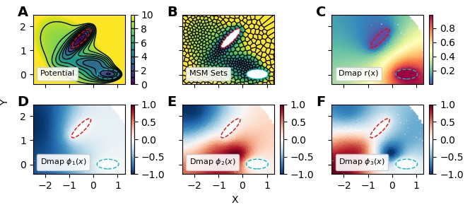
Figure 1: Example basis and guess functions constructed by the diffusion-map basis on the scaled Müller-Brown potential. (A) The potential energy surface. Black contour lines indicate the potential energy in units of $k_{B}T$, red and cyan dotted contours indicate the boundaries of states $A$ and $B$ respectively. (B) An MSM clustering with 500 sets on the domain; the color scale is the same as in (A). Each MSM basis function is one inside a cell and zero otherwise. Sets inside states A and B are not shown to emphasize the boundary conditions. (C) Scatter plot of the guess function for the committor for hitting $B$ before $A$, constructed using (58). (D–F) Scatter plots of the first three basis functions constructed according to (57).

Diffusion maps are a technique shown to have success in finding global descriptions of molecular systems from high-dimensional input data.Ferguson et al. (2010); Rohrdanz et al. (2011); Zheng et al. (2011); Ferguson et al. (2011); Long and Ferguson (2014); Kim et al. (2015) A simple implementation proceeds by constructing the transition matrix

$$P^{\rm DMAP}_{mn}=\frac{K_{\varepsilon}(x_{m},x_{n})}{\sum_{n}K_{\varepsilon}(x_{m},x_{n})},$$ (56)

where $K_{\varepsilon}$ is a kernel function that decays exponentially with the distance between datapoints $x_{m}$ and $x_{n}$ at a rate set by $\varepsilon$. Multiple choices of $K_{\varepsilon}$ exist; we give the algorithm used to construct the kernel in the Supplementary Information in Section X.2. The eigenvectors of $P^{\rm DMAP}$ with $M$ highest positive eigenvalues were historically used to define a new coordinate system for dimensionality reduction. They can also be used as a basis set for DOEA and similar analyses.Boninsegna et al. (2015); Berry, Giannakis, and Harlim (2015); Giannakis (2017) Here we extend this line of research, showing that diffusion maps can also be used to construct basis functions that obey homogeneous boundary conditions on arbitrary sets as required for use in DGA. We note that the diffusion process represented by $P^{\rm DMAP}$ is not intended as an approximation of the dynamics, but rather as a tool for building the basis functions $\phi_{i}$. In particular, while the $P^{\rm DMAP}$ matrix is typically reversible, this imposes no reversible constraint in the DGA scheme using the basis derived from $P^{\rm DMAP}$.

To construct a basis set that obeys nontrivial boundary conditions, we first take the submatrix of $P^{\rm DMAP}$ such that $x_{m},x_{n}\in D$. We then calculate the eigenvectors $\varphi_{i}$ of this submatrix that have the $M$ highest positive eigenvalues, and take as our basis

$$\phi_{i}(x)=\begin{cases}\varphi_{i}(x)\text{ for }x\text{ in }D,\\ 0\text{ otherwise}.\end{cases}$$ (57)

In addition to allowing us to define a basis set, $P^{\rm DMAP}$ gives a natural way of constructing guess functions that obey the boundary conditions. Since (56) is a transition matrix, it corresponds to a discrete Markov chain on the data. Therefore, we can construct guesses by solving analogs to (33) using the dynamics specified by the diffusion map. For equations using the generator, we solve the problem

$$\sum_{n}(P^{\rm DMAP}-I)_{mn}r_{n} =h(x_{m})\text{ for }m\text{ in }D$$ (58)

$$r_{m} =b(x_{m})\text{ for }m\text{ in }D^{c}$$ (59)

where $I$ is the identity matrix. Here the sum runs over all datapoints, not just those in $D$. The resulting estimate obeys the boundary conditions for all datapoints sampled in $D^{c}$.

Equation (58) can also be used to construct guesses for equations using weighted adjoints. In principle, one could replace $P^{\rm DMAP}$ with its weighted adjoint against $p$ and solve the corresponding equation. However, $r_{n}$ still obeys the boundary conditions irrespective of the weighted adjoint used. We therefore take the adjoint of $P^{\rm DMAP}$ with respect to its stationary measure. Since the Markov chain associated with the diffusion map is reversible,Coifman and Lafon (2006) $P^{\rm DMAP}$ is self-adjoint with respect to its stationary measure and we again solve (58). We discuss how to perform out-of-sample extension on the basis and the guess functions in the Supplementary Information in Section X.2.

To help the reader visualize a diffusion-map basis, we analyze a collection of datapoints sampled from the Müller-Brown potential,Müller and Brown (1979) scaled by 20 so that the barrier height is about 7 energy units; we set $k_{B}T=1$. This potential is sampled using a Brownian particle with isotropic diffusion coefficient of $0.1$ using the BAOAB integrator for overdamped dynamics with a time step of 0.01 time units.Leimkuhler and Matthews (2012) Trajectories are initialized out of the stationary measure by uniformly picking 10000 starting locations on the interval $x\in\left(-2.5,1.5\right),y\in\left(-2.5,1.5\right)$. Initial points with potential energies larger than $100$ are rejected and resampled to avoid numerical artifacts. Each trajectory is then constructed by simulating the dynamics for 500 steps, saving the position every 100 steps.

We then define two states $A$ and $B$ (red and cyan dashed contours in Figure 1, respectively) and construct the basis and guess functions required for the committor. The results, plotted in Figure 1, demonstrate that the diffusion-map basis functions are smoothly varying with global support.

V.1 Basis Set Performance in High-Dimensional CV spaces.

We now test the effect of dimension on the performance of the basis set by attempting to calculate the forward committor and total reactive flux for a series of toy systems based on the model above. To be able to vary the dimensionality of the system, we add up to $18$ harmonic “nuisance” degrees of freedom. Specifically,

$$U\left(x,y,z_{3},...,z_{d}\right)=U_{\rm MB}(x,y)+\sum_{l=3}^{d}z_{l}^{2},$$ (60)

where $U_{\rm MB}$ is the scaled Müller-Brown potential discussed above. We compare our results with references computed by a grid-based scheme described in the Supplementary Information. Our reference for the committor is plotted in Figure 3A. We initialize the $x$ and $y$ dimensions as above; the initial values of the nuisance coordinates were drawn from their marginal distributions at equilibrium. We then sampled the system using the same procedure as before.

Throughout this section and all subsequent numerical comparisons, we compare the diffusion-map basis with a basis of indicator functions. Since, with minor restrictions, using a basis of indicator functions is equivalent to calculating the same dynamical quantities using a MSM, we estimate committors, mean first-passage times, and stationary distributions by constructing a MSM in PyEMMA and using established formulas.Metzner, Schütte, and Vanden-Eijnden (2009); Noé and Prinz (2014); Keller, Aleksic, and Donati (2019) In general, it is not our intention to compare an optimal diffusion-map basis to an optimal MSM basis. Multiple diffusion-map and clustering schemes exist and performing an exhaustive comparison would require comparison over multiple methods and hyperparameters. We leave such a comparison for future work, and only seek to present reasonable examples of both schemes.

MSM clusters are constructed using $k$-means, as implemented in PyEMMA.Scherer et al. (2015) While MSMs are generally constructed by clustering points globally, this does not guarantee that a given clustering satisfies a specific set of boundary conditions. Consequently, we modify the set definition procedure slightly.

We first construct $M$ clusters on the domain $D$, and then cluster $D^{c}$ separately. The number of states inside $D^{c}$ is chosen so that states inside $D^{c}$ have approximately the same number of samples on average as states in the domain. For the current calculation, this corresponded to approximately one state inside set $A$ or $B$ for every five states outside the domain; we round to a ratio of $1/5$ for numerical simplicity. We note that clustering on the interior of $D^{c}$ does not affect calculated committors or mean first-passage times. We use 500 basis functions for both the MSM and diffusion-map basis sets. We give plots supporting this choice in Section X.5 of the Supplementary Information.

In modern Markov state modeling, one commonly constructs the transition matrix only over a well-connected subset of states named the active set.Prinz et al. (2011); Beauchamp et al. (2011) We have follow this practice, and exclude points outside the active set from any error analyses of the resulting MSMs. We believe this gives the MSM basis an advantage over the diffusion-map basis in our comparisons, as we are explicitly ignoring points where it fails to provide an answer and would presumably give poor results.

It is also common to ensure that the resulting matrix obeys detailed balance through a maximum likelihood procedure.Bowman et al. (2009); Prinz et al. (2011) We choose not to do this because we do not wish to assume reversibility in our formalism. Moreover, our calculations have also shown that enforcing reversibility can introduce a statistical bias that dominates the error in any estimates. We give numerical examples of this phenomenon in Section X.6 of the Supplementary Information.

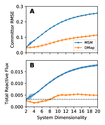
Figure 2: Comparison of basis performance the dimensionality of the toy system increases. (A) The average error in the forward committor between states $B$ and $A$ in Figure 3 for both the MSM and the diffusion-map basis functions, as a function of the number of nuisance degrees of freedom. (B) Estimated reactive using both MSM and the diffusion-map basis functions as function of the same. In both plots shading indicates the standard deviation over 30 datasets. The dotted line in (B) is the reactive flux as calculated by an accurate reference scheme.

In Figure 2A, we plot root-mean-square error (RMSE) between the estimated and reference forward committors as a function of the number of nuisance degrees of freedom. While for low-dimensional systems the MSM and the diffusion-map basis give comparable results, as we increase the dimensionality, the MSM gives increasingly worse answers.

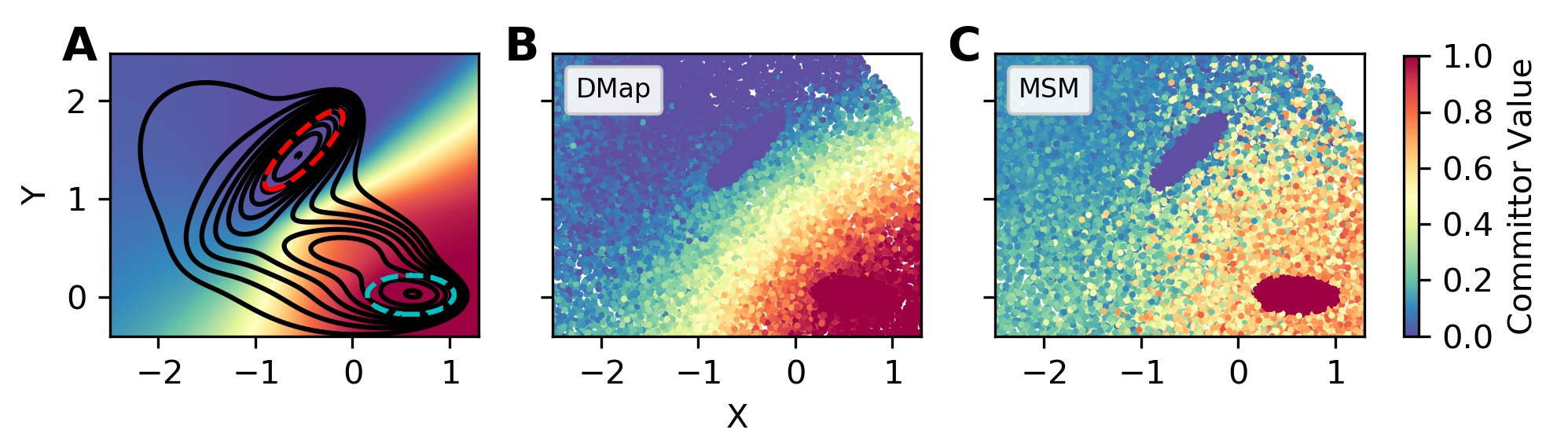
Figure 3: Example forward committors calculated using the diffusion-map and MSM bases on a high-dimensional toy problem. The system is the same as in Figure 1, with 18 additional nuisance dimensions. (A) Forward committor function calculated using an accurate grid-based scheme. The black lines indicate the contours of free energy in the $x$ and $y$ coordinates, and the red and cyan dashed contours indicate the two states. Every subsequent dimension has a harmonic potential with force constant of 2. (B–C) Estimated forward committor constructed using the diffusion map and MSM bases, respectively.

To aid in understanding these results, we plot example forward committor estimates for the 20-dimensional system in Figure 3. We see that the diffusion-map basis manages to capture the general trends in the reference in Figure 3A. In contrast, the MSM basis gives considerably noisier results.

We also estimate the total reactive flux across the same dataset, setting $C$ and $C^{c}$ in (83) to be the sets on either side of the calculated isocommittor (Figure 2B). The large errors that we observe in the reactive flux occur due to the nature of the dataset. If data were collected from a long equilibrium trajectory, it would not be necessary to estimate $\pi(x)$ separately, and we could set $\pi(x)=1$. In that case, provided the number of MSM states was sufficient, the MSM reactive flux reverts to direct estimation of the number of reactive trajectories per unit time. This would give an accurate reactive flux regardless of the quality of the estimated forwards or backwards committors.

VI Addressing Projection Error Through Delay Embedding

Our results suggest that improving basis set choice can yield DGA schemes with better accuracy in higher-dimensional CV spaces. However, even large CV spaces are considerably lower-dimensional than the system’s full state space. Consequently, they may still omit key degrees of freedom needed to describe the long-time dynamics. In both MSMs and DOEA, this projection error is often addressed by increasing the lag time of the transition operator.Prinz et al. (2011); Suárez, Adelman, and Zuckerman (2016); Nüske et al. (2016); Mardt et al. (2018) This is based on the assumption that degrees of freedom omitted from the CV space equilibrate quickly and contribute little to the long-time dynamics. However, there is no guarantee that this assumption holds for any specific choice of CVs. This is reflected by existing bounds on the approximation error for DOEA. For instance, the relative error in the estimate of the dominant eigenvalue is bounded above by the projection error of the basis onto the dominant eigenfunction; this bound does not decrease with the lag time.Djurdjevac, Sarich, and Schütte (2012)

Moreover, whereas changing the lag time does not affect the eigenfunctions in (6), the equations in Section III hold only for a lag time of $\Delta t$. Using a longer time is effectively making the approximation

$$\mathcal{L}f(x)\approx\frac{\mathcal{K}_{s}f(x)-f(x)}{s}.$$ (61)

This causes a systematic bias in the estimates of the dynamical quantities discussed in Section III. While for small lag times this bias is likely negligible, it may become large as the lag time increases. For instance, estimates of the mean first-passage time grow linearly with $s$ as the lag time goes to infinity.Suárez, Adelman, and Zuckerman (2016)

Here, we propose an alternative strategy for dealing with projection error. Rather than looking at larger time lags, we use past configurations in CV space to account for contributions from the removed degrees of freedom. This idea is central to the Mori-Zwanzig formalism.Zwanzig (2001) Here, we use delay embedding to include history information. Let $\zeta^{(t)}$ be the projection of $\Xi^{(t)}$ at time $t$. We define the delay-embedded process with $d$ delays as

$$\theta^{(t)}=\left(\zeta^{(t)},\zeta^{(t-\Delta t)},\zeta^{(t-2\Delta t)},\ldots,\zeta^{(t-d\Delta t)}\right).$$ (62)

Delay embedding has a long history in the study of deterministic, finite-dimensional systems, where it has been shown that delay embedding can recapture attractor manifolds up to diffeomorphism.Takens (1981); Aeyels (1981) Weaker mathematical results have been extended to stochastic systems,Muldoon et al. (1998); Stark et al. (1997) although these are not sufficient to guarantee its effectiveness in all cases.

Delay embedding has been used previously with dimensionality reduction on both experimentalBerry et al. (2013) and simulated chemical systems,Wang and Ferguson (2016, 2018) and has also been used in applications of DOEA in geophysics.Giannakis (2017) In references Giannakis, 2017; Fung et al., 2016 it was argued that delay embedding can improve statistical accuracy for noise-corrupted and time-uncertain data. Other methods of augmenting the dynamical process with history information have been used in the construction of MSMs. In reference Suarez et al., 2014, each trajectory was augmented with a labeling variable indicating its origin state. In reference Suárez, Adelman, and Zuckerman, 2016, it was suggested to write transition probabilities as a function of both the current and the preceding MSM state. This corresponds to a specific choice of basis on a delay embedded process.

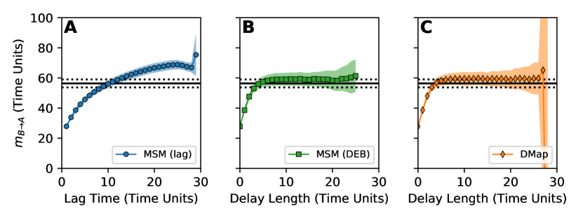
Figure 4: Comparison of methods for dealing with the projection error in an incomplete CV space. In all subplots we estimate the mean first-passage time from state $B=\left\{y<0.15\right\}$ to state $A=\left\{y>1.15\right\}$ using a DGA scheme on only the $y$ coordinate of the Müller-Brown potential. (A) Estimate constructed using an MSM basis with increasing lag time in (61), as a function of the lag time. (B) Estimate constructed using an MSM basis, but applying delay embedding rather than increasing the lag time, as a function of the delay length. (C) Estimate constructed using the diffusion-map basis with delay embedding, as a function of the delay length. In each plot, the symbols show the mean over 30 identically constructed trajectories, and the shading indicates the standard deviation across trajectories. The black solid line is an estimate of the mean first-passage time calculated using the reference scheme in the Supplementary Information, and the dashed error bars represent the standard deviation of the mean first-passage time over state $B$.

Here we show that delay embedding can be used to improve dynamical estimates in DGA. To apply DGA to the delay-embedded process, we must extend the functions $h$ and $b$ in (33) and (33) to the delay-embedded space. We do this by using the value of the function on the central timepoint,

$$f\left(\theta^{(t)}\right)=f\left(\zeta^{(t-\lfloor d/2\rfloor\Delta t}\right)$$ (63)

where $\lfloor\ldots\rfloor$ denotes rounding down to the nearest integer. The states $D$ and $D^{c}$ in the delay-embedded space are extended similarly. One can easily show that this preserves dynamical quantities such as mean first-passage times and committors. The basis set is then constructed directly on $\theta$, and the DGA formalism is applied as before.

We test the effect of delay embedding in the presence of projection error by constructing DGA schemes on the same system as in Section V and taking as our CV space only the $y$-coordinate. For this study we revise our dataset to include 2000 trajectories, each sampled for 3000 time steps. While using longer trajectories changes the density such that it is closer to equilibrium, it allows us to test longer lag times and delay lengths. To ensure that our states are well-defined in this new CV space, we redefine state $A$ to be the set $\{y>1.15\}$, and state $B$ to be the set $\{y<0.15\}$. We then estimate the mean first-passage time into state $A$, conditioned on starting in state $B$ at equilibrium.

$$m_{B\to A}=\frac{\int\mathds{1}_{B}(x)m_{A}(x)\pi(x)\mu(dx)}{\int\mathds{1}_{B}(x)\pi(x)\mu(dx)}.$$

We construct estimates using an MSM basis with varying lag time, an MSM basis with delay embedding, and a diffusion-map basis with delay embedding.

In Figure 4, we plot the average mean first-passage time as a function of the lag time and the trajectory length used in the delay embedding. We compare the resulting estimates with an estimate of the mean first-passage time constructed using our grid-based scheme. In addition, an implied timescale analysis for the two MSM schemes is given in the Supplementary Information in Section X.7.

The mean first-passage time estimated from the MSM basis with the lag time steadily increases as the lag time becomes longer (Figure 4A), as predicted in reference Suárez, Adelman, and Zuckerman, 2016. In contrast, the estimates obtained from delay embedding both converge as the delay length increases, albeit to a value slightly larger than the reference. We believe this small error is because we treat the dynamics as having a discrete time step, while the reference curve approximates the mean first-passage time for a continuous-time Brownian dynamics. In particular, The latter includes events in which the system enters and exits the target state within the duration of a discrete-time time step, but such events are missing from the discrete-time dynamics.

In all three schemes, we see anomalous behavior as the length of the lag time or delay length increases. This is due to an increase in statistical error when the delay length or lag time becomes close to the length of the trajectory. If each trajectory has $N$ datapoints, performing a delay-embedding with $d$ delays means that each trajectory only gives $N-d$ samples. When $N$ and $d$ are of the same order of magnitude, this leads to increased statistical error in the estimates in IV.3, to the point of making the resulting linear algebra problem ill-posed. The diffusion-map basis fluctuates to unreasonable values at long delay lengths, and the MSM basis fails completely, truncating the curve in Figures 4B and C. Similarly, the lagged MSM has an anomalous downturn in the average mean first-passage time near 26 time units. We give additional plots supporting this theory in the Supplementary Information in Section X.7.

Finally, we observe that the delay length required for the estimate to converge is substantially smaller than the mean first-passage time. This suggests that delay embedding can be effectively used on short trajectories to get estimates of long-time quantities.

VII Application to the Fip35 WW Domain

To further assess our methods, we now apply them to molecular dynamics data and seek to evaluate committors and mean first-passage times. In contrast to the simulations above, we do not have accurate reference values and cannot directly calculate the error in our estimates. Instead, we observe that both the mean first-passage time and forward committor are conditional expectations, and obey the following relations Durrett (2010)

$$m_{A}(x)= \operatorname*{arg\,min}_{f(x)}\mathrm{\mathbf{E}}\left[\left(\tau_{A}-f(x)\right)^{2}\right]$$

$$q_{+}(x)= \operatorname*{arg\,min}_{f(x)}\mathrm{\mathbf{E}}\left[\left(\mathbf{1}_{\tau_{B}<\tau_{A}}-f(x)\right)^{2}\right].$$

This suggests a scheme for assessing the quality of our estimates. If we have access to long trajectories, each point in the trajectory has an associated sample of $\tau_{A}$ and $\mathbf{1}_{\tau_{B}<\tau_{A}}$. We define the two empirical cost functions

$$\text{COST}_{m_{A}}= \frac{1}{N}\sum_{n=1}^{N}(\bar{m}_{A}(x_{n})-\tau_{{A},n})^{2}$$ (64)

$$\text{COST}_{q_{+}}= \frac{1}{N}\sum_{n=1}^{N}(\bar{q}_{+}(x_{n})-\mathbf{1}_{{\tau_{B}<\tau_{A}},n})^{2}.$$ (65)

Here $x_{n}$ is a collection of samples from a long trajectory, $\tau_{{A},n}$ is the time from $x_{n}$ to $A$, and $\mathbf{1}_{{\tau_{B}<\tau_{{A},n}}}$ is one if the sampled trajectory next reaches $B$ and zero if it next reaches $A$. The numerical estimates of the mean first-passage time and committor are written as $\bar{m}_{A}$ and $\bar{q}$, respectively. In the limit of $N\to\infty$, the true mean first-passage time and committor would minimize (64) and (65). We consequently expect lower values of our cost functions to indicate improved estimates. For a perfect estimate, however, these cost functions would not go to zero. Rather, in the limit of infinite sampling, (64) and (65) would converge to the variances of $\tau_{A}$ and $\mathbf{1}_{\tau_{B}<\tau_{A}}$. For the procedure to be valid, it is important that the cost estimates are not constructed using the same dataset used to build the dynamical estimates. This avoids spurious correlations between the dynamical estimate and the estimated cost.

We applied our methods to the Fip35 WW domain trajectories described by D.E. Shaw Research in references Shaw et al., 2010; Piana et al., 2011. The dataset consists of six trajectories, each of length 100000 ns with frames output every 0.2 ns. Each trajectory has multiple folding and unfolding events, allowing us to evaluate the empirical cost functions. To avoid correlations between the DGA estimate and the calculated cost, we perform a test/train split and divide the data into two halves. We choose three trajectories to construct our estimate, and use the other three to approximate the expectations in (64) and (65). Repeating this for each possible choice of trajectories creates a total of 20 unique test/train splits.

To reduce the memory requirements in constructing the diffusion map kernel matrix, we subsampled the trajectories, keeping every 100th frame. This allowed us to test the scheme over a broad range of hyperparameters. We expect that in practical applications a finer time resolution would be used, and any additional computational expense could be offset by using landmark diffusion maps.Long and Ferguson (2017)

To define the folded and unfolded states, we follow reference Berezovska, Prada-Gracia, and Rao, 2013 and calculate $r_{\beta 1}$ and $r_{\beta 1}$, the minimum root-mean-square-displacement for each of the two $\beta$ hairpins, defined as amino acids 7-23 and 18-29, respectively.Berezovska, Prada-Gracia, and Rao (2013) We define the folded configuration as having both $r_{\beta 1}<0.2$ nm and $r_{\beta 2}<0.13$ nm and the unfolded configuration as having $0.4$ nm $<r_{\beta 1}<1.0$ nm and $0.3$ nm $<r_{\beta 2}<0.75$ nm. For convenience, we refer to these states as $A$ and $B$ throughout this section. We then attempt to estimate the forward committor between the two states and the mean first-passage time into $A$ using the same methods as in Section VI.

We take as our CVs the pairwise distances between every other $\alpha$-carbon, leading to a 153-dimensional space. In previous studies, dimensionality-reduction schemes such as TICA have been applied prior to MSM construction. We choose not to do this, as we are interested in the performance of the schemes in large CV spaces. This also helps control the number of hyperparameters and algorithm design choices, although we think the interaction between dimensionality-reduction schemes and families of basis sets merits future investigation.

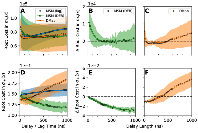
Figure 5: Results from a DGA calculation on a dataset of six long folding and unfolding trajectories of the Fip35 WW domain. (A,D) The root cost in the mean first-passage time and forward committor respectively, calculated using an MSM basis with increasing lag time, an MSM basis with delay embedding, and diffusion map basis with delay embedding, averaged over all test/train splits. (B,C,E,F) Difference in root cost relative to the best parameter choice for the estimate constructed using the MSM basis with increasing lag time. Negative values are better. (B) Difference in cost for the mean first-passage time estimated with an MSM basis with delay embedding. (C) The same as in (B) but with the diffusion map basis instead. (E) Difference in cost for the committor estimated with an MSM basis with delay embedding. (F) The same as in (E) but with the diffusion map basis instead. In all plots the symbols are the average over test/train splits, and the shading indicates the standard deviation across test/train splits.

Our results are given in Figure 5. In panels A and B, we give the mean value of the cost for the mean first-passage time and forward committor over all test/train splits, as calculated using 200 basis functions for each algorithm. The number of basis functions was chosen to give the best result for the MSM scheme with increasing lag over any lag time, although we see only very minor differences in behavior for larger basis sets. The large standard deviations primarily reflect variation in the cost across different test/train splits, rather than any difference between the methods. This suggests the presence of large numerical noise in our results.

To get a more accurate comparison, we instead look at the expected improvement in cost between schemes for a given test/train split. To quantify whether an improvement occurs, we first determine the best parameter choice for the MSM basis with increasing lag. We estimate the cost for the MSM basis with delay embedding and for the diffusion-map basis, and calculate the difference in cost versus the lagged MSM scheme for each test/train split. We then average and calculate the standard deviation over pairs, and plot the results in figures 5C through 5F. As the difference is calculated against the best parameter choice for the lagged MSM scheme, they are intrinsically conservative: in practice, one should not expect to have the optimal lagged MSM parameters.

In our numerical experiments, we see that the diffusion map seems to give the best results for relatively short delay lengths. However, the diffusion-map basis performs progressively worse as the delay length increases. The mechanism causing this loss in accuracy requires further analysis. This tentatively suggests the use of the diffusion-map basis for datasets consisting of very short trajectories, where using long delays may be infeasible. In contrast, our results with the delay-embedded MSM basis are more ambiguous. For the mean first-passage time, we do not see significant improvement over the results from the lagged MSM results. We do see noticeable improvement in the estimated forward committor probability as the delay length increases. However, we observe that the delay lengths required to improve upon the diffusion map result are comparable in magnitude to the average time required for the trajectory to reach either the $A$ or $B$ states. Indeed, we only see an improvement over the diffusion-map result at a delay length of 180 ns, and we observe that the longest the trajectory spends outside of both state $A$ or state $B$ is 223 ns. This negates any advantage of using datasets of short trajectories.

Caution is warranted in interpreting these results. We see large variances between different test/train splits, suggesting that despite having 300 $\mu s$ of data in each training dataset, we are still in a relatively data-poor regime. Similarly, we cannot make an authoritative recommendation for any particular scheme for calculating dynamical quantities without further research. Such a study would not only require more simulation data, but also a comparison of multiple clustering and diffusion map schemes across several hyperparameters and their interaction with various dimensionality-reduction schemes. We leave this task for future work. However, our initial results are promising, suggesting that further development of DGA schemes and basis sets is warranted.

VIII Conclusions

In this paper, we introduce a new framework for estimating dynamical statistics from trajectory data. We express the quantity of interest as the solution to an operator equation using the generator or one of its adjoints. We then apply a Galerkin approximation, projecting the unknown function onto a finite-dimensional basis set. This allows us to approximate the problem as a system of linear equations, whose matrix elements we approximate using Monte Carlo integration on dynamical data. We refer to this framework as Dynamical Galerkin Approximation (DGA). These estimates can be constructed using collections of short trajectories initialized from relatively arbitrary distributions. Using a basis set of indicator functions on nonoverlapping sets recovers MSM estimates of dynamical quantities. Our work is closely related to existing work on estimating the eigenfunctions of dynamical operators in a data-driven manner.

To demonstrate the utility of alternative basis sets, we introduce a new method for constructing basis functions based on diffusion maps. Results on a toy system shows that this basis has the potential to give improved results in high-dimensional CV spaces. We also combine our formalism with delay-embedding, a technique for recovering degrees of freedom omitted in constructing a CV space. Applying it to an incomplete, one-dimensional projection of our test system, we see that delay embedding can improve on the current practice of increasing the lag time of the dynamical operator.

We then applied the method to long folding trajectories of the Fip35 WW domain to study the performance of the schemes in a large CV space on a nontrivial biomolecule. Our results suggest that the diffusion-map basis gives the best performance for short delay times, giving results that are as good or better than the best time-lagged MSM parameter choice. Moreover, our results suggest that combining the MSM basis with delay embedding gives promising results, particularly for long delay lengths. However, long delay lengths are required to see an improvement over the diffusion-map basis, potentially negating any computational advantage in using short trajectories to estimate committors and mean first-passage times.

We believe our work raises new theoretical and algorithmic questions. Most immediately, we hope our preliminary numerical results motivate the need for new approaches to building basis sets and guess functions obeying the necessary boundary conditions. Further theoretical work is also required to assess the validity of using delay embedding in our schemes. Finally, we believe it is worth searching for connections between our work and VAC and VAMP theory.Noé and Nüske (2013); Nüske et al. (2014, 2016); Wu and Noé (2017); Mardt et al. (2018) In particular, a variational reformulation of the DGA scheme would allow substantially more flexible representation of solutions. With these further developments, we believe DGA schemes have the potential to give further improved estimates of dynamical quantities for difficult molecular problems.

IX Acknowledgements

This work was supported by National Institutes of Health Award R01 GM109455 and by the Molecular Software Sciences Institute (MolSSI) Software Fellows program. Computing resources where provided by the University of Chicago Research Computing Center (RCC). The Fip35 WW domain data was provided by D.E. Shaw Research. Most of this work was completed while JW was a member of the Statistics Department and the James Franck Institute at the University of Chicago. We thank Charles Matthews, Justin Finkel, and Benoit Roux for helpful discussions, as well as Fabian Paul, Frank Noé, and the anonymous reviewers for their constructive feedback on earlier versions of the manuscript.

X Supplementary Information

X.1 Connection between DGA and Markov State Modeling

Here, we describe in detail the connection between DGA and certain dynamical estimates calculated using a MSM.

To map the general dynamics onto the state space of the Markov Chain, we make three assumptions.

Assumption X.1.

Each Markov state $S_{i}$ is contained entirely in either $D$ or in $D^{c}$.

Assumption X.2.

The boundary conditions $b$ can be expressed as

$$b(x)=\sum_{l\in D^{c}}^{M^{\prime}}b_{l}\mathds{1}_{S_{l}}(x).$$ (66)

Assumption X.3.

For any $\mathcal{L}_{p}^{\dagger}$ considered, $p$ can be written as

$$p(x)=\sum_{j\in D}^{M}\frac{p_{j}}{\left\langle\mathds{1}_{j}\right\rangle}\mathds{1}_{j}(x)+\sum_{l\in D^{c}}^{M^{\prime}}\frac{p_{l}}{\left\langle\mathds{1}_{l}\right\rangle}s\mathds{1}_{l}(x).$$ (67)

The first assumption is necessary for the basis set to obey the homogeneous boundary conditions, and can be enforced explicitly in the construction of the MSM. The second two assumptions will be required to make the action of $\mathcal{L}$ representable as the action of matrices on vectors over the MSM states. While these assumptions should not be expected to hold for general $b$ and $p$, in the correct limit of infinite sampling and sufficiently small Markov states, we expect (66) and (67) to be arbitrarily good approximations. In fact, for most $b$ in Section III, assumption X.2 can hold exactly. We also note that the vector $p_{i}$ sums to one, as

$$1= \int p(x)\mu(dx)$$

$$= \int\sum_{j\in D}^{M}\frac{p_{j}}{\left\langle\mathds{1}_{j}\right\rangle}\mathds{1}_{j}(x)+\sum_{l\in D^{c}}^{M^{\prime}}\frac{p_{l}}{\left\langle\mathds{1}_{l}\right\rangle}\mathds{1}_{l}(x)\mu(dx)$$

$$= \sum_{j\in D}^{M}p_{j}+\sum_{l\in D^{c}}^{M^{\prime}}p_{l}.$$

Consequently, $p_{i}$ is a probability distribution over the MSM state-space.

X.1.1 Equations with the Transition Operator

We first consider equations that take the form of (33). As our guess, we will use (38). Substituting into (42), applying Assumption X.2, and dividing by $\left\langle 1_{S_{i}}\right\rangle$, we arrive at

$$\sum_{j\in D}^{M}\frac{1}{\Delta t}\left(P-I\right)_{ij}a_{j}=\eta_{i}-\sum_{l\in D^{c}}^{M^{\prime}}\frac{1}{\Delta t}\left(P-I\right)_{il}b_{l}.$$ (68)

Here $P_{ij}$ is the MSM transition matrix defined in (3) with a time lag of $\Delta t$, and $\eta_{i}$ is defined as

$$\eta_{i}=\frac{\left\langle\mathds{1}_{i},h\right\rangle}{\left\langle\mathds{1}_{i}\right\rangle}$$ (69)

This can be rewritten as

$$\begin{split}\sum_{j}\frac{1}{\Delta t}\left(P-I\right)_{ij}a_{j}&=\eta_{i}\text{ for }i\in D\\ a_{i}&=b_{i}\text{ for }i\in D^{c}\end{split}$$ (70)

where the sum is over states on the entire domain. This is equivalent to (33) for the dynamics given by the MSM.

X.1.2 Equations with Transition Adjoints

For equations that take the form of (34) we again begin with (42), this time with terms defined by equations (48), (50), and (49). Substituting in our guess function and Assumptions X.3 and X.1, we have

$$\begin{split}\sum_{j\in D}^{M}\left\langle\mathcal{L}\mathds{1}_{i},\mathds{1}_{j}\right\rangle&\left(\frac{p_{j}}{\left\langle\mathds{1}_{j}\right\rangle}\right)a_{j}\\ =\left(\frac{p_{i}}{\left\langle\mathds{1}_{i}\right\rangle}\right)&\left\langle\mathds{1}_{i},h\right\rangle-\sum_{l\in D^{c}}^{M^{\prime}}\left\langle\mathcal{L}\mathds{1}_{i},\mathds{1}_{l}\right\rangle b_{l}\left(\frac{p_{l}}{\left\langle\mathds{1}_{l}\right\rangle}\right)\end{split}$$ (71)

We then divide both sides by $p_{i}$. Applying the definition of $P_{ij}$, we arrive at

$$\sum_{j\in D}^{M}p_{i}^{-1}\left(P-I\right)_{ij}^{T}p_{j}a_{j}=\eta_{i}-\sum_{l\in D^{c}}^{M^{\prime}}p_{i}^{-1}\left(P-I\right)_{il}p_{l}b_{l}.$$ (72)

which, as before, is equivalent to solving

$$\begin{split}\sum_{j}p_{i}^{-1}\left(P-I\right)^{T}_{ij}p_{j}&=\eta_{i}\text{ for }i\in D\\ a_{i}&=b_{i}\text{ for }i\in D^{c}.\end{split}$$ (73)

Comparing with (26), we see that the matrix with elements $p_{i}^{-1}\left(P-I\right)_{ij}^{T}p_{j}$ is the weighted adjoint of the MSM generator against $p_{i}$. Consequently, (73) is equivalent to (34) for the MSM.

X.2 Details of Diffusion Map Construction

Here, we give the specific kernel and parameter choice used in our calculations used to construct the diffusion map in our calculations. Our procedure closely follows work in references Berry, Giannakis, and Harlim, 2015 and Berry and Harlim, 2016. Specifically, our algorithm corresponds to the parameter choice $\alpha=0$ and $\beta=-1/d$ in reference Berry and Harlim, 2016 and not performing the bandwidth normalization in equation (5).

X.2.1 Kernel Construction

As in Section V, let $x_{m}$ be a collection of $N$ datapoints. We define the initial bandwidth function

$$\varsigma_{0}(x_{m})=\frac{1}{k_{0}}\sum_{l=1}^{k_{0}}||x_{m}-x_{I(m,l)}||^{2}$$

where $I(m,l)$ is the index of the $l$’th nearest neighbor to point $x_{m}$ (not including $x_{m}$). Here $k_{0}$ is a neighborhood parameter giving the number of nearest neighbors considered, we follow reference Berry and Harlim, 2016 and set it to 7. We then construct the kernel density estimate

$$\begin{split}q(x_{m})=\frac{(2\pi\varepsilon_{0})^{-d/2}}{N\varsigma_{0}(x_{m})^{d}}\sum_{n=1}^{N}K_{0}(x_{m},x_{n};\varepsilon_{0})\text{, where}\\ K_{0}(x_{m},x_{n};\varepsilon_{0})=\exp\left(\frac{-||x_{m}-x_{n}||^{2}}{2\varepsilon_{0}\varsigma_{0}(x_{m})\varsigma_{0}(x_{n})}\right)\end{split}$$

where $d$ is the intrinsic dimensionality of the data manifold and $\varepsilon_{0}$ is a bandwidth parameter. To estimate $d$ and a good choice for $\varepsilon_{0}$, we consider all possible choices of $eps_{0}$ of the form $2^{k}$ with $k=-40,-39,\dots,39,40$. We then set

$$d=\frac{2}{\ln(2)}\max_{k}\left[\ln\left(\frac{\sum_{m,n}K_{0}(x_{m},x_{n},2^{k+1})}{\sum_{m,n}K_{0}(x_{m},x_{n},2^{k})}\right)\right]$$ (74)

Reference Berry, Giannakis, and Harlim, 2015 suggests setting $\varepsilon_{0}$ by using the $k$ where the right-hand-side attains its maximum. In practice we find this can be overly aggressive, so we subsequently multiply $\varepsilon_{0}$ by 2. We then construct the Diffusion map kernel matrix as

$$K(x_{m},x_{n})=\exp\left(\frac{||x-y||^{2}}{\varepsilon q(x_{m})^{-1/d}q(x_{n})^{-1/d}}\right)$$ (75)

where we select the $\varepsilon$ using the same procedure as before.

X.2.2 Out-of-sample Extension for the Diffusion-Map Basis

To predict the values of the quantities in Section III at new datapoints, we will need to extend the diffusion-map basis and guess functions to new configurations. Initially, one might attempt this by constructing a new diffusion map matrix that contains both the old and the new points and recomputing the guess and eigenvectors. However, not only would this procedure be expensive, it would change the values of the basis and guess functions on the old points. Consequently, the estimates of $a_{j}$ would be incorrect, and the entire DGA scheme would need to be repeated. We therefore seek a method for extending the basis and guess functions to new points that leave their values on older points unchanged.

Let $x_{\nu}$ be a new point added to the dataset. To extend the basis functions to $x_{\nu}$, we can use the established method of Nyström extension.Williams and Seeger (2001); Long and Ferguson (2017) Let $\varphi_{i}$ be an eigenvector of the submatrix discussed in Section V, and let $\kappa_{i}$ be the associated eigenvalue. The estimate of the basis function on $x_{\nu}$ is given by

$$\varphi_{i}(x_{\nu})=\frac{1}{\kappa_{i}}\frac{\sum_{m}K_{\varepsilon}(x_{m},x_{\nu})\varphi_{i}(x_{m})}{\sum_{m}K_{\varepsilon}(x_{m},x_{\nu})}$$ (76)

To extend the guess function to new configurations, we introduce a new method based on the Jacobi method.Bronshtein et al. (2007) We first consider $\hat{P}$, a new diffusion map matrix built using both the old datapoints $x_{1..N}$ and the new datapoint $x_{\nu}$. The guess function associated with $\hat{P}$ would then solve the problem

$$\left(\hat{P}-I\right)g=h$$ (77)

for all of the points in $D$. We will construct our estimate of $g$ at the new point by considering a single iteration of the Jacobi method for solving (77). Our initial vector takes values of $g_{m}$ on $x_{m}$ and $0$ on $x_{\nu}$. This gives us the following out-of-sample extension formula

$$g_{\nu}=\frac{1}{\hat{P}_{\nu\nu}-1}\left(h_{\nu}-\sum_{m=1}^{N}\hat{P}_{\nu m}g_{m}\right)$$ (78)

where the sum runs only over points in the original dataset. This can be further simplified using the definition of $\hat{P}$ to

$$g_{\nu}=\frac{\sum_{m=1}^{N}K_{\varepsilon}\left(x_{\nu},x_{m}\right)g_{m}}{\sum_{m=1}^{N}K_{\varepsilon}\left(x_{\nu},x_{m}\right)}-h_{\nu}\left(1+\frac{K_{\varepsilon}\left(x_{\nu},x_{\nu}\right)}{\sum_{m=1}^{N}K_{\varepsilon}\left(x_{\nu},x_{m}\right)}\right).$$ (79)

X.3 Derivation of Transition Path Theory Reactive Flux and Rate in Discrete Time

Transition path theory was originally formulated for diffusion processesVanden-Eijnden (2006) and was extended to finite-state Markov jump processes.Metzner, Schütte, and Vanden-Eijnden (2009) Here, we derive analogous equations for discrete-time Markov chains on arbitrary state spaces. The derivation closely follows reference Vanden-Eijnden, 2006. Let $x(t)$ be a single trajectory ergodically sampling the stationary measure. We will extend the trajectory both forwards and backwards in time so the time index $t$ takes values from $-\infty$ to $\infty$. For all $t$, let

$$t_{AB}^{+}(t) =\min\left\{t^{\prime}|t^{\prime}\geq t,x(t^{\prime})\in A\cup B\right\}$$ (80)

$$t_{AB}^{-}(t) =\max\left\{t^{\prime}|t^{\prime}\leq t,x(t^{\prime})\in A\cup B\right\}$$ (81)

be the next time the system entered $A$ or $B$ and the most recent time the system left $A$ or $B$, respectively. Now let $C$ be as in (28). The total reactive current is defined as

$$I_{B\to A}= \lim_{T\to\infty}\frac{1}{2T}\sum_{t\in[-T,T]}\left[\mathds{1}_{C}\left(x(t)\right)\mathds{1}_{C^{c}}\left(x(t+\Delta t)\right)\right.$$

$$\qquad\qquad-\left.\mathds{1}_{C^{c}}\left(x(t)\right)\mathds{1}_{C}\left(x(t+\Delta t)\right)\right]$$ (82)

$$\qquad\qquad\left[\mathds{1}_{A}\left(x(t_{AB}^{-}(t)\right)\mathds{1}_{B}\left(x(t_{AB}^{+}(t+\Delta t)\right)\right]$$

Using ergodicity and the strong Markov property, we can rewrite this as an average against $\rho_{\Delta t}$.

$$I_{B\to A}= \int\mathds{1}_{C^{c}}(y)q_{+}(y)q_{-}(x)\mathds{1}_{C}(x)\pi(x)\rho_{\Delta t}(dx,dy)$$ (83)

$$-\int\mathds{1}_{C}(y)q_{+}(y)q_{-}(x)\mathds{1}_{C^{c}}(x)\pi(x)\rho_{\Delta t}(dx,dy)$$

This is the discrete-time equivalent of equation (30) in reference Vanden-Eijnden, 2006. Applying the definition of the generator and observing that that $\mathds{1}_{C}(x)\mathds{1}_{C^{c}}(x)=0$ everywhere gives (28). We then arrive at (29) in our work by the same arguments as in reference E and Vanden-Eijnden, 2010.

X.4 Grid-Based Reference Scheme

Here we discuss the scheme used to calculate the reference values for our test system in Sections V and VI. Instead of considering the discrete time process directly, we will attempt to approximate the dynamics of the continuous-time Brownian dynamics on the test potential. To this end, we define a Markov hopping process on a grid that converges to the continuous time dynamics as the grid becomes finer. Specifically, we allow nearest neighbor hops on a square grid with spacing $\epsilon$. The hopping probabilities are given by

$$P(x+\epsilon,y)= \left(\frac{1}{4}\right)\left(\frac{1}{1+\exp\left[U(x+\epsilon,y)-U(x,y)\right]}\right)$$

$$P(x-\epsilon,y)= \left(\frac{1}{4}\right)\left(\frac{1}{1+\exp\left[U(x-\epsilon,y)-U(x,y)\right]}\right)$$

$$P(x,y+\epsilon)= \left(\frac{1}{4}\right)\left(\frac{1}{1+\exp\left[U(x,y+\epsilon)-U(x,y)\right]}\right)$$ (85)

$$P(x,y-\epsilon)= \left(\frac{1}{4}\right)\left(\frac{1}{1+\exp\left[U(x,y-\epsilon)-U(x,y)\right]}\right)$$

$$P(x,y)= 1-P(x+\epsilon,y)-P(x-\epsilon,y)$$

$$-P(x,y+\epsilon)-P(x,y-\varepsilon).$$

Here $P(x\pm\epsilon,y)$ is the probability of hopping one grid point to the right or left, $P(x,y\pm\epsilon)$ is the probability of hopping up or down the grid, and $P(x,y)$ is the probability of remaining in place.

We will not give a full proof of convergence. Instead we merely demonstrate that as $\epsilon\to 0$, we approximate the infinitesimal generator $\mathcal{L}^{\rm brwn}$ for Brownian Dynamics. Let $P$ be the transition matrix associated with the transition probabilities given by (X.4), $f$ be a three-times continuously differentiable function, and the vector $\vec{f}$ the values of $f$ evaluated at each grid point. In the limit of $\epsilon\to 0$,

$$\frac{16(P-I)\vec{f}}{\epsilon^{2}}(x,y)=\mathcal{L}^{\rm brwn}f(x,y)+\mathcal{O}(\epsilon)$$ (86)

where $\mathcal{L}^{\rm brwn}$ is the infinitesimal generator for Brownian dynamics with isotropic diffusion constant,

$$\mathcal{L}^{\rm brwn}f(x,y)= -\partial_{x}U(x,y)\partial_{x}f(x,y)-\partial_{y}U(x,y)\partial_{y}f(x,y)$$

$$+\partial_{x}^{2}f(x,y)+\partial_{y}^{2}f(x,y).$$

To demonstrate this, we write $(P-I)\vec{f}$ explicitly as

$$(P-I)f(x,y)= P(x+\epsilon,y)f(x+\epsilon,y)$$

$$+P(x-\epsilon,y)f(x-\epsilon,y)$$

$$+P(x,y+\epsilon)f(x,y+\epsilon)$$

$$+P(x,y-\epsilon)f(x,y-\epsilon)$$

$$+P(x,y)f(x,y)+\mathcal{O}(\epsilon^{3})$$

If we expand $f$ to second order around $(x,y)$, the zeroth order term cancels, leaving

$$(P-I)f(x,y)= P(x+\epsilon,y)\left(\epsilon\partial_{x}f+\frac{1}{2}\epsilon^{2}\partial^{2}_{x}f\right)$$

$$-P(x-\epsilon,y)\left(\epsilon\partial_{x}f-\frac{1}{2}\epsilon^{2}\partial^{2}_{x}f\right)$$

$$+P(x,y+\epsilon r)\left(\epsilon\partial_{y}f+\frac{1}{2}(\epsilon r)^{2}\partial^{2}_{y}f\right)$$

$$-P(x,y-\epsilon r)\left(\epsilon\partial_{y}f-\frac{1}{2}(\epsilon r)^{2}\partial^{2}_{y}f\right)+\mathcal{O}(\epsilon^{3})$$

We then expand the transition probabilities to first order, giving

$$P(x\pm\epsilon,y) =\frac{1}{8}\left(1\mp\frac{1}{2}\partial_{x}U(x,y)\epsilon\right)+\mathcal{O}(\epsilon^{2})$$

$$P(x,y\pm\epsilon r) =\frac{1}{8}\left(1\mp\frac{1}{2}\partial_{x}U(x,y)\epsilon\right)+\mathcal{O}(\epsilon^{2}).$$

Substituting, simplifying, and multiplying by $16/\epsilon^{2}$ gives (86).

To estimate the reference quantities for our test system, we constructed a square grid on the interval $-2.5\leq x\leq 1.5$ and $-1.5\leq y\leq 2.5$ with grid spacing of 0.005. We then construct the transition rate matrix $16(P-I)/\epsilon^{2}$, and estimate the dynamical quantities using the corresponding formulas in Section III.

X.5 Basis Size Choice for Müller-Brown model

In Figure 6, we show the dependence of the root-mean-square error in the committor on basis size for the Müller-Brown model. While using 1000 basis functions gives a slightly better result at higher dimensions, it is not enough to appreciably change the trends depicted in Figure 2. However, choosing 1000 or more basis functions gives worse results for the two-dimensional system. We therefore chose to use $500$ dimensions to avoid giving the impression that the diffusion-map basis outperforms the MSM basis at low dimensions.

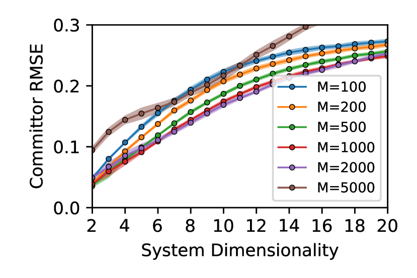
Figure 6: Dependence of the MSM committor root-mean-square error (RMSE) on the number of clusters. Different curves correspond to different numbers of Markov states.

X.6 Numerical Effect of Enforcing Detailed Balance

To test the effect of enforcing detailed balance in MSMs through a maximum likelihood procedure, we returned to our two-dimensional test potential without any additional nuisance degrees of freedom. Using the clusterings described in Section V.1, we constructed MSMs in PyEMMA both with and without the reversible option set to True. We then estimated the mean first-passage time from state $B$ into state $A$, using the states depicted in Figure 1A. As before, we repeated this procedure over thirty replicates. Moreover, we also varied the number of short trajectories included in the dataset to observe trends in statistical convergence.

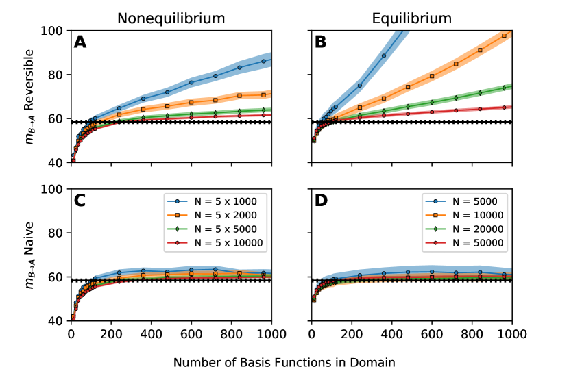
Figure 7: Effect of enforcing MSM reversibility on the estimated mean first-passage time from state $B$ to state $A$ on the scaled Müller-Brown potential. Estimates in the top row are constructed using the reversible MSM estimator and estimates in the bottom row are not. The columns correspond to two different datasets: the left column shows estimates constructed from the nonequilibrium dataset detailed in section V, and the right column shows estimates constructed from a long equilibrium trajectory. Different curves correspond to MSMs constructed from datasets of different sizes.

Our results are given in Figure 7. The mean first-passage time calculated using reversible MSMs, depicted in panel A, grows unboundedly with increasing basis size. To demonstrate that this not due to the nature of the data, we repeated the calculation on a long equilibrium trajectory of commensurate length. Our results, shown in panel B, exhibit the same phenomenon. We also varied the error tolerance for convergence, as well as the minimum count required for connectivity. Neither affected the results. Moreover, an in-house code for the iteration described in reference Bowman et al., 2009 gave the same results as PyEMMA. Rather, we see that the bias decays with increasing dataset sizes, suggesting that it is statistical in nature.

In panels C and D, we show estimates constructed without enforcing reversibility, which we term the naive estimator. The naive estimator does not have the same bias. This suggests that the maximum likelihood iteration introduces a large, slowly decaying statistical error.

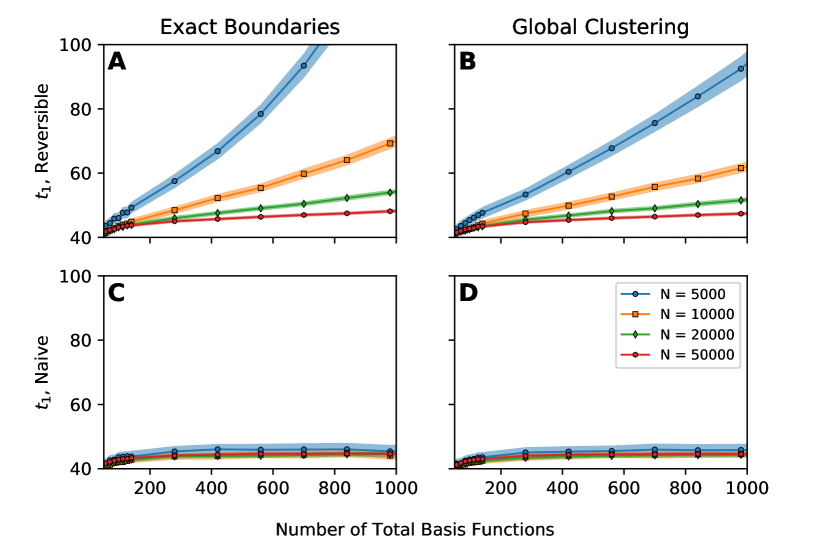
Figure 8: Dominant implied timescale for MSMs constructed on a long equilibrium trajectory on the scaled Müller-Brown potential. Estimates in the top row are constructed using the reversible MSM estimator and estimates in the bottom row use the naive estimator. Columns correspond two different clustering schemes. The left column gives estimates constructed using the clustering described in Section V.1, and the right column gives estimates obtained by clustering the data without regard for the boundary conditions (i.e., globally). Different curves correspond to MSMs constructed on different size datasets.

To ensure that this is not an artifact of the clustering procedure, we also constructed MSMs by applying $k$-means globally to the data, without regard to boundary conditions. We then estimated the dominant implied timescale for both clustering schemes, which we plot in Figure 8. We see the same trends as in the mean first-passage time: for reversible MSMs, the implied timescale grows unboundedly with the number of basis functions for both clustering methods. In contrast, both clustering methods converge equally well when using the naive estimator.

X.7 Supplementary Plots for Delay Embedding the Müller-Brown model

In Figure 9, we give implied timescales for the MSMs constructed in Section VI.

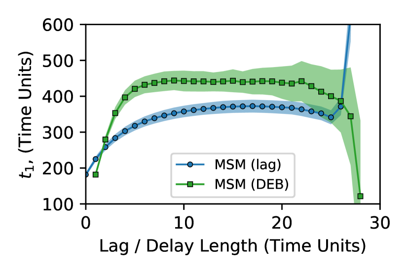
Figure 9: Implied timescales for the delay-embedded MSM and lagged MSMs in Section VI.

To test the effect of trajectory length on the one-dimensional, delay-embedded data, we repeated the calculation for three additional datasets. The total number of points in each dataset is fixed, but each nonequilibrium trajectory is of different length. We plot the resulting curves in Figure 10. In all cases, we see an anomalous behavior when the delay length or lag time approaches the total length of the trajectory.

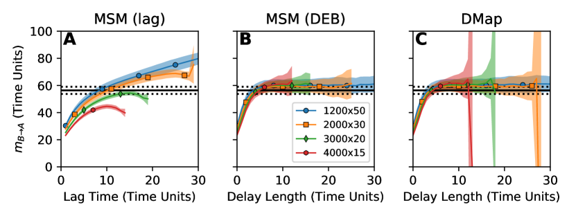
Figure 10: Comparison of methods for controlling the projection error in an incomplete CV space. Plots are as in Figure 4, with the addition of three new datasets. The curves correspond to datasets consisting of 1200 trajectories, each 50 time units long (blue circles), 200 points, each 30 time units long (orange squares, the same data as pictured in Figure 4), 3000 trajectories, each 20 units long (green diamonds), and 4000 trajectories, each 15 units long (red hexagons).

References

- Kramers (1940) H. A. Kramers, “Brownian motion in a field of force and the diffusion model of chemical reactions,” Physica 7, 284–304 (1940).
- Hänggi, Talkner, and Borkovec (1990) P. Hänggi, P. Talkner, and M. Borkovec, “Reaction-rate theory: fifty years after Kramers,” Reviews of Modern Physics 62, 251 (1990).
- Vanden-Eijnden (2006) E. Vanden-Eijnden, “Transition path theory,” in Computer Simulations in Condensed Matter Systems: From Materials to Chemical Biology Volume 1 (Springer, 2006) pp. 453–493.
- Berezhkovskii et al. (2014) A. M. Berezhkovskii, A. Szabo, N. Greives, and H.-X. Zhou, “Multidimensional reaction rate theory with anisotropic diffusion,” The Journal of Chemical Physics 141, 11B616_1 (2014).
- Ma, Nag, and Dinner (2006) A. Ma, A. Nag, and A. R. Dinner, “Dynamic coupling between coordinates in a model for biomolecular isomerization,” The Journal of chemical physics 124, 144911 (2006).
- Ovchinnikov, Nam, and Karplus (2016) V. Ovchinnikov, K. Nam, and M. Karplus, “A simple and accurate method to calculate free energy profiles and reaction rates from restrained molecular simulations of diffusive processes,” The Journal of Physical Chemistry B 120, 8457–8472 (2016).
- Ghysels et al. (2017) A. Ghysels, R. M. Venable, R. W. Pastor, and G. Hummer, “Position-dependent diffusion tensors in anisotropic media from simulation: oxygen transport in and through membranes,” Journal of chemical theory and computation 13, 2962–2976 (2017).
- Dinner and Karplus (1999) A. R. Dinner and M. Karplus, “The thermodynamics and kinetics of protein folding: a lattice model analysis of multiple pathways with intermediates,” The Journal of Physical Chemistry B 103, 7976–7994 (1999).
- Dinner et al. (2000) A. R. Dinner, A. Šali, L. J. Smith, C. M. Dobson, and M. Karplus, “Understanding protein folding via free-energy surfaces from theory and experiment,” Trends in Biochemical Sciences 25, 331–339 (2000).
- Dellago et al. (1998) C. Dellago, P. G. Bolhuis, F. S. Csajka, and D. Chandler, “Transition path sampling and the calculation of rate constants,” The Journal of Chemical Physics 108, 1964–1977 (1998).
- Bolhuis et al. (2002) P. G. Bolhuis, D. Chandler, C. Dellago, and P. L. Geissler, “Transition path sampling: Throwing ropes over rough mountain passes, in the dark,” Annual Review of Physical Chemistry 53, 291–318 (2002).
- Grünwald, Dellago, and Geissler (2008) M. Grünwald, C. Dellago, and P. L. Geissler, “Precision shooting: Sampling long transition pathways,” The Journal of Chemical Physics 129, 194101 (2008).
- Gingrich and Geissler (2015) T. R. Gingrich and P. L. Geissler, “Preserving correlations between trajectories for efficient path sampling,” The Journal of Chemical Physics 142, 06B614_1 (2015).
- Huber and Kim (1996) G. A. Huber and S. Kim, “Weighted-ensemble Brownian dynamics simulations for protein association reactions,” Biophysical Journal 70, 97 (1996).
- van Erp, Moroni, and Bolhuis (2003) T. S. van Erp, D. Moroni, and P. G. Bolhuis, “A novel path sampling method for the calculation of rate constants,” The Journal of Chemical Physics 118, 7762–7774 (2003).
- Faradjian and Elber (2004) A. K. Faradjian and R. Elber, “Computing time scales from reaction coordinates by milestoning,” The Journal of Chemical Physics 120, 10880–10889 (2004).
- Allen, Frenkel, and ten Wolde (2006) R. J. Allen, D. Frenkel, and P. R. ten Wolde, “Simulating rare events in equilibrium or nonequilibrium stochastic systems,” The Journal of chemical physics 124, 024102 (2006).
- Warmflash, Bhimalapuram, and Dinner (2007) A. Warmflash, P. Bhimalapuram, and A. R. Dinner, “Umbrella sampling for nonequilibrium processes,” The Journal of Chemical Physics 127, 114109 (2007).
- Vanden-Eijnden and Venturoli (2009) E. Vanden-Eijnden and M. Venturoli, “Exact rate calculations by trajectory parallelization and tilting,” The Journal of chemical physics 131, 044120 (2009).
- Dickson, Warmflash, and Dinner (2009) A. Dickson, A. Warmflash, and A. R. Dinner, “Separating forward and backward pathways in nonequilibrium umbrella sampling,” The Journal of Chemical Physics 131, 154104 (2009).
- Guttenberg, Dinner, and Weare (2012) N. Guttenberg, A. R. Dinner, and J. Weare, “Steered transition path sampling,” The Journal of Chemical Physics 136, 06B609 (2012).
- Bello-Rivas and Elber (2015) J. M. Bello-Rivas and R. Elber, “Exact milestoning,” The Journal of Chemical Physics 142, 03B602_1 (2015).
- Dinner et al. (2018) A. R. Dinner, J. C. Mattingly, J. O. Tempkin, B. V. Koten, and J. Weare, “Trajectory stratification of stochastic dynamics,” SIAM Review 60, 909–938 (2018).
- Schütte et al. (1999) C. Schütte, A. Fischer, W. Huisinga, and P. Deuflhard, “A direct approach to conformational dynamics based on hybrid Monte Carlo,” Journal of Computational Physics 151, 146–168 (1999).
- Swope, Pitera, and Suits (2004) W. C. Swope, J. W. Pitera, and F. Suits, “Describing protein folding kinetics by molecular dynamics simulations. 1. Theory,” The Journal of Physical Chemistry B 108, 6571–6581 (2004).
- Pande, Beauchamp, and Bowman (2010) V. S. Pande, K. Beauchamp, and G. R. Bowman, “Everything you wanted to know about Markov state models but were afraid to ask,” Methods 52, 99–105 (2010).
- Sarich, Noé, and Schütte (2010) M. Sarich, F. Noé, and C. Schütte, “On the approximation quality of Markov state models,” Multiscale Modeling & Simulation 8, 1154–1177 (2010).
- Noé and Fischer (2008) F. Noé and S. Fischer, “Transition networks for modeling the kinetics of conformational change in macromolecules,” Current Opinion in Structural Biology 18, 154–162 (2008).
- Noé and Prinz (2014) F. Noé and J.-H. Prinz, “Analysis of Markov models,” in An Introduction to Markov State Models and Their Application to Long Timescale Molecular Simulation, vol. 797 of Advances in Experimental Medicine and Biology, edited by G. R. Bowman, V. S. Pande, and F. Noé (Springer, 2014) Chap. 6.
- Keller, Aleksic, and Donati (2019) B. G. Keller, S. Aleksic, and L. Donati, “Markov state models in drug design,” in Biomolecular Simulations in Drug Discovery, edited by F. L. Gervasio and V. Spiwok (Wiley-VCH, 2019) Chap. 4.
- Weber (2006) M. Weber, Meshless Methods in Conformation Dynamics, Ph.D. thesis, Freie Universität Berlin (2006).
- Noé and Nüske (2013) F. Noé and F. Nüske, “A variational approach to modeling slow processes in stochastic dynamical systems,” Multiscale Modeling & Simulation 11, 635–655 (2013).
- Eisner et al. (2015) T. Eisner, B. Farkas, M. Haase, and R. Nagel, Operator Theoretic Aspects of Ergodic Theory, Vol. 272 (Springer, 2015).
- Klus et al. (2018) S. Klus, F. Nüske, P. Koltai, H. Wu, I. Kevrekidis, C. Schütte, and F. Noé, “Data-driven model reduction and transfer operator approximation,” Journal of Nonlinear Science 28, 985–1010 (2018).
- Billingsley (2008) P. Billingsley, Probability and Measure (John Wiley & Sons, 2008).
- Bowman et al. (2009) G. R. Bowman, K. A. Beauchamp, G. Boxer, and V. S. Pande, “Progress and challenges in the automated construction of Markov state models for full protein systems,” The Journal of Chemical Physics 131, 124101 (2009).
- Prinz et al. (2011) J.-H. Prinz, H. Wu, M. Sarich, B. Keller, M. Senne, M. Held, J. D. Chodera, C. Schütte, and F. Noé, “Markov models of molecular kinetics: Generation and validation,” The Journal of Chemical Physics 134, 174105 (2011).
- Noé et al. (2009) F. Noé, C. Schütte, E. Vanden-Eijnden, L. Reich, and T. R. Weikl, “Constructing the equilibrium ensemble of folding pathways from short off-equilibrium simulations,” Proceedings of the National Academy of Sciences 106, 19011–19016 (2009).
- Schwantes and Pande (2013) C. R. Schwantes and V. S. Pande, “Improvements in Markov state model construction reveal many non-native interactions in the folding of NTL9,” Journal of Chemical Theory and Computation 9, 2000–2009 (2013).
- Pérez-Hernández et al. (2013) G. Pérez-Hernández, F. Paul, T. Giorgino, G. De Fabritiis, and F. Noé, “Identification of slow molecular order parameters for Markov model construction,” The Journal of Chemical Physics 139, 07B604_1 (2013).
- Schwantes, McGibbon, and Pande (2014) C. R. Schwantes, R. T. McGibbon, and V. S. Pande, “Perspective: Markov models for long-timescale biomolecular dynamics,” The Journal of Chemical Physics 141, 09B201 (2014).
- Schütte and Sarich (2015) C. Schütte and M. Sarich, “A critical appraisal of Markov state models,” The European Physical Journal Special Topics 224, 2445–2462 (2015).
- Shukla et al. (2015) D. Shukla, C. X. Hernández, J. K. Weber, and V. S. Pande, “Markov state models provide insights into dynamic modulation of protein function,” Accounts of Chemical Research 48, 414–422 (2015).
- Berezovska, Prada-Gracia, and Rao (2013) G. Berezovska, D. Prada-Gracia, and F. Rao, “Consensus for the Fip35 folding mechanism?” The Journal of Chemical Physics 139, 07B608_1 (2013).
- Sheong et al. (2014) F. K. Sheong, D.-A. Silva, L. Meng, Y. Zhao, and X. Huang, “Automatic state partitioning for multibody systems (APM): an efficient algorithm for constructing Markov state models to elucidate conformational dynamics of multibody systems,” Journal of Chemical Theory and Computation 11, 17–27 (2014).
- Li and Dong (2016) Y. Li and Z. Dong, “Effect of clustering algorithm on establishing Markov state model for molecular dynamics simulations,” Journal of Chemical Information and Modeling 56, 1205–1215 (2016).
- Husic and Pande (2017) B. E. Husic and V. S. Pande, “Ward clustering improves cross-validated Markov state models of protein folding,” Journal of Chemical Theory and Computation 13, 963–967 (2017).
- Husic et al. (2018) B. E. Husic, K. A. McKiernan, H. K. Wayment-Steele, M. M. Sultan, and V. S. Pande, “A minimum variance clustering approach produces robust and interpretable coarse-grained models,” Journal of Chemical Theory and Computation 14, 1071–1082 (2018).
- Steinbach, Ertöz, and Kumar (2004) M. Steinbach, L. Ertöz, and V. Kumar, “The challenges of clustering high dimensional data,” in New Directions in Statistical Physics (Springer, 2004) pp. 273–309.
- Kriegel, Kröger, and Zimek (2009) H.-P. Kriegel, P. Kröger, and A. Zimek, “Clustering high-dimensional data: A survey on subspace clustering, pattern-based clustering, and correlation clustering,” ACM Transactions on Knowledge Discovery from Data (TKDD) 3, 1 (2009).
- Scherer et al. (2015) M. K. Scherer, B. Trendelkamp-Schroer, F. Paul, G. Pérez-Hernández, M. Hoffmann, N. Plattner, C. Wehmeyer, J.-H. Prinz, and F. Noé, “PyEMMA 2: a software package for estimation, validation, and analysis of Markov models,” Journal of Chemical Theory and Computation 11, 5525–5542 (2015).
- Molgedey and Schuster (1994) L. Molgedey and H. G. Schuster, “Separation of a mixture of independent signals using time delayed correlations,” Physical Review Letters 72, 3634 (1994).
- Takano and Miyashita (1995) H. Takano and S. Miyashita, “Relaxation modes in random spin systems,” Journal of the Physical Society of Japan 64, 3688–3698 (1995).
- Hirao, Koseki, and Takano (1997) H. Hirao, S. Koseki, and H. Takano, “Molecular dynamics study of relaxation modes of a single polymer chain,” Journal of the Physical Society of Japan 66, 3399–3405 (1997).
- Schütte et al. (2011) C. Schütte, F. Noé, J. Lu, M. Sarich, and E. Vanden-Eijnden, “Markov state models based on milestoning,” The Journal of Chemical Physics 134, 05B609 (2011).
- Giannakis, Slawinska, and Zhao (2015) D. Giannakis, J. Slawinska, and Z. Zhao, “Spatiotemporal feature extraction with data-driven Koopman operators,” in Feature Extraction: Modern Questions and Challenges (2015) pp. 103–115.
- Giannakis (2017) D. Giannakis, “Data-driven spectral decomposition and forecasting of ergodic dynamical systems,” Applied and Computational Harmonic Analysis (2017).
- Williams, Kevrekidis, and Rowley (2015) M. O. Williams, I. G. Kevrekidis, and C. W. Rowley, “A data–driven approximation of the Koopman operator: Extending dynamic mode decomposition,” Journal of Nonlinear Science 25, 1307–1346 (2015).
- Boninsegna et al. (2015) L. Boninsegna, G. Gobbo, F. Noé, and C. Clementi, “Investigating molecular kinetics by variationally optimized diffusion maps,” Journal of Chemical Theory and Computation 11, 5947–5960 (2015).
- Vitalini, Noé, and Keller (2015) F. Vitalini, F. Noé, and B. Keller, “A basis set for peptides for the variational approach to conformational kinetics,” Journal of Chemical Theory and Computation 11, 3992–4004 (2015).
- Wu and Noé (2017) H. Wu and F. Noé, “Variational approach for learning Markov processes from time series data,” arXiv preprint arXiv:1707.04659 (2017).
- Mardt et al. (2018) A. Mardt, L. Pasquali, H. Wu, and F. Noé, “VAMPnets for deep learning of molecular kinetics,” Nature Communications 9, 5 (2018).
- Nüske et al. (2014) F. Nüske, B. G. Keller, G. Pérez-Hernández, A. S. Mey, and F. Noé, “Variational approach to molecular kinetics,” Journal of Chemical Theory and Computation 10, 1739–1752 (2014).
- Nüske et al. (2016) F. Nüske, R. Schneider, F. Vitalini, and F. Noé, “Variational tensor approach for approximating the rare-event kinetics of macromolecular systems,” The Journal of Chemical Physics 144, 054105 (2016).
- Prinz, Chodera, and Noé (2014) J.-H. Prinz, J. D. Chodera, and F. Noé, “Spectral rate theory for two-state kinetics,” Physical Review X 4, 011020 (2014).
- Del Moral (2004) P. Del Moral, Feynman-Kac Formulae (Springer, 2004).
- Karatzas and Shreve (2012) I. Karatzas and S. Shreve, Brownian Motion and Stochastic Calculus, Vol. 113 (Springer Science & Business Media, 2012).
- Du et al. (1998) R. Du, V. S. Pande, A. Y. Grosberg, T. Tanaka, and E. S. Shakhnovich, “On the transition coordinate for protein folding,” The Journal of Chemical Physics 108, 334–350 (1998).
- Bolhuis, Dellago, and Chandler (2000) P. G. Bolhuis, C. Dellago, and D. Chandler, “Reaction coordinates of biomolecular isomerization,” Proceedings of the National Academy of Sciences 97, 5877–5882 (2000).
- Metzner, Schütte, and Vanden-Eijnden (2009) P. Metzner, C. Schütte, and E. Vanden-Eijnden, “Transition path theory for Markov jump processes,” Multiscale Modeling & Simulation 7, 1192–1219 (2009).
- Yosida (1971) K. Yosida, “Functional analysis, 1980,” Spring-Verlag, New York/Berlin (1971).
- Lapelosa and Abrams (2013) M. Lapelosa and C. F. Abrams, “Transition-path theory calculations on non-uniform meshes in two and three dimensions using finite elements,” Computer Physics Communications 184, 2310–2315 (2013).
- Lai and Lu (2018) R. Lai and J. Lu, “Point cloud discretization of Fokker–Planck operators for committor functions,” Multiscale Modeling & Simulation 16, 710–726 (2018).
- Khoo, Lu, and Ying (2018) Y. Khoo, J. Lu, and L. Ying, “Solving for high dimensional committor functions using artificial neural networks,” arXiv preprint arXiv:1802.10275 (2018).
- Evans (1998) L. Evans, Partial Differential Equations (Orient Longman, 1998).
- Thiede (2018) E. Thiede, “PyEDGAR,” https://github.com/ehthiede/PyEDGAR/ (2018).
- Wu et al. (2017) H. Wu, F. Nüske, F. Paul, S. Klus, P. Koltai, and F. Noé, “Variational Koopman models: slow collective variables and molecular kinetics from short off-equilibrium simulations,” The Journal of Chemical Physics 146, 154104 (2017).
- Chen, Tu, and Rowley (2012) K. K. Chen, J. H. Tu, and C. W. Rowley, “Variants of dynamic mode decomposition: boundary condition, Koopman, and Fourier analyses,” Journal of nonlinear science 22, 887–915 (2012).
- Coifman and Lafon (2006) R. R. Coifman and S. Lafon, “Diffusion maps,” Applied and Computational Harmonic Analysis 21, 5–30 (2006).
- Berry and Harlim (2016) T. Berry and J. Harlim, “Variable bandwidth diffusion kernels,” Applied and Computational Harmonic Analysis 40, 68–96 (2016).
- Ferguson et al. (2010) A. L. Ferguson, A. Z. Panagiotopoulos, P. G. Debenedetti, and I. G. Kevrekidis, “Systematic determination of order parameters for chain dynamics using diffusion maps,” Proceedings of the National Academy of Sciences 107, 13597–13602 (2010).
- Rohrdanz et al. (2011) M. A. Rohrdanz, W. Zheng, M. Maggioni, and C. Clementi, “Determination of reaction coordinates via locally scaled diffusion map,” The Journal of Chemical Physics 134, 03B624 (2011).
- Zheng et al. (2011) W. Zheng, B. Qi, M. A. Rohrdanz, A. Caflisch, A. R. Dinner, and C. Clementi, “Delineation of folding pathways of a -sheet miniprotein,” The Journal of Physical Chemistry B 115, 13065–13074 (2011).
- Ferguson et al. (2011) A. L. Ferguson, A. Z. Panagiotopoulos, I. G. Kevrekidis, and P. G. Debenedetti, “Nonlinear dimensionality reduction in molecular simulation: The diffusion map approach,” Chemical Physics Letters 509, 1–11 (2011).
- Long and Ferguson (2014) A. W. Long and A. L. Ferguson, “Nonlinear machine learning of patchy colloid self-assembly pathways and mechanisms,” The Journal of Physical Chemistry B 118, 4228–4244 (2014).
- Kim et al. (2015) S. B. Kim, C. J. Dsilva, I. G. Kevrekidis, and P. G. Debenedetti, “Systematic characterization of protein folding pathways using diffusion maps: Application to trp-cage miniprotein,” The Journal of Chemical Physics 142, 02B613_1 (2015).
- Berry, Giannakis, and Harlim (2015) T. Berry, D. Giannakis, and J. Harlim, “Nonparametric forecasting of low-dimensional dynamical systems,” Physical Review E 91, 032915 (2015).
- Müller and Brown (1979) K. Müller and L. D. Brown, “Location of saddle points and minimum energy paths by a constrained simplex optimization procedure,” Theoretica Chimica Acta 53, 75–93 (1979).
- Leimkuhler and Matthews (2012) B. Leimkuhler and C. Matthews, “Rational construction of stochastic numerical methods for molecular sampling,” Applied Mathematics Research eXpress 2013, 34–56 (2012).
- Beauchamp et al. (2011) K. A. Beauchamp, G. R. Bowman, T. J. Lane, L. Maibaum, I. S. Haque, and V. S. Pande, “MSMBuilder2: Modeling conformational dynamics on the picosecond to millisecond scale,” Journal of Chemical Theory and Computation 7, 3412–3419 (2011).
- Suárez, Adelman, and Zuckerman (2016) E. Suárez, J. L. Adelman, and D. M. Zuckerman, “Accurate estimation of protein folding and unfolding times: beyond Markov state models,” Journal of Chemical Theory and Computation 12, 3473–3481 (2016).
- Djurdjevac, Sarich, and Schütte (2012) N. Djurdjevac, M. Sarich, and C. Schütte, “Estimating the eigenvalue error of Markov state models,” Multiscale Modeling & Simulation 10, 61–81 (2012).
- Zwanzig (2001) R. Zwanzig, Nonequilibrium Statistical Mechanics (Oxford University Press, 2001).
- Takens (1981) F. Takens, “Detecting strange attractors in turbulence,” Lecture Notes in Mathematics 898, 366–381 (1981).
- Aeyels (1981) D. Aeyels, “Generic observability of differentiable systems,” SIAM Journal on Control and Optimization 19, 595–603 (1981).
- Muldoon et al. (1998) M. R. Muldoon, D. S. Broomhead, J. P. Huke, and R. Hegger, “Delay embedding in the presence of dynamical noise,” Dynamics and Stability of Systems 13, 175–186 (1998).
- Stark et al. (1997) J. Stark, D. Broomhead, M. Davies, and J. Huke, “Takens embedding theorems for forced and stochastic systems,” Nonlinear Analysis: Theory, Methods & Applications 30, 5303–5314 (1997).
- Berry et al. (2013) T. Berry, J. R. Cressman, Z. Greguric-Ferencek, and T. Sauer, “Time-scale separation from diffusion-mapped delay coordinates,” SIAM Journal on Applied Dynamical Systems 12, 618–649 (2013).
- Wang and Ferguson (2016) J. Wang and A. L. Ferguson, “Nonlinear reconstruction of single-molecule free-energy surfaces from univariate time series,” Physical Review E 93, 032412 (2016).
- Wang and Ferguson (2018) J. Wang and A. L. Ferguson, “Recovery of protein folding funnels from single-molecule time series by delay embeddings and manifold learning,” The Journal of Physical Chemistry B 122, 11931–11952 (2018).
- Fung et al. (2016) R. Fung, A. M. Hanna, O. Vendrell, S. Ramakrishna, T. Seideman, R. Santra, and A. Ourmazd, “Dynamics from noisy data with extreme timing uncertainty,” Nature 532, 471 (2016).
- Suarez et al. (2014) E. Suarez, S. Lettieri, M. C. Zwier, C. A. Stringer, S. R. Subramanian, L. T. Chong, and D. M. Zuckerman, “Simultaneous computation of dynamical and equilibrium information using a weighted ensemble of trajectories,” Journal of Chemical Theory and Computation 10, 2658–2667 (2014).
- Durrett (2010) R. Durrett, Probability: Theory and Examples (Cambridge university press, 2010).
- Shaw et al. (2010) D. E. Shaw, P. Maragakis, K. Lindorff-Larsen, S. Piana, R. O. Dror, M. P. Eastwood, J. A. Bank, J. M. Jumper, J. K. Salmon, Y. Shan, and W. Wriggers, “Atomic-level characterization of the structural dynamics of proteins,” Science 330, 341–346 (2010).
- Piana et al. (2011) S. Piana, K. Sarkar, K. Lindorff-Larsen, M. Guo, M. Gruebele, and D. E. Shaw, “Computational design and experimental testing of the fastest-folding -sheet protein,” Journal of Molecular Biology 405, 43–48 (2011).
- Long and Ferguson (2017) A. W. Long and A. L. Ferguson, “Landmark diffusion maps (L-dMaps): Accelerated manifold learning out-of-sample extension,” Applied and Computational Harmonic Analysis (2017).
- Williams and Seeger (2001) C. K. Williams and M. Seeger, “Using the Nyström method to speed up kernel machines,” in Advances in Neural Information Processing Systems (2001) pp. 682–688.
- Bronshtein et al. (2007) I. Bronshtein, K. Semendyayev, G. Musiol, and H. Muehlig, Handbook of Mathematics, 3rd ed. (Springer, 2007).
- E and Vanden-Eijnden (2010) W. E and E. Vanden-Eijnden, “Transition-path theory and path-finding algorithms for the study of rare events,” Annual Review of Physical Chemistry 61, 391–420 (2010).