Multi-time Formulation of Matsubara Dynamics

Abstract

Matsubara dynamics has recently emerged as the most general form of a quantum-Boltzmann-conserving classical dynamics theory for the calculation of single-time correlation functions. Here, we present a generalization of Matsubara dynamics for the evaluation of multi-time correlation functions. We show that the Matsubara approximation can also be used to approximate the two-time symmetrized double Kubo transformed correlation function. By a straightforward extension of these ideas to the multi-time realm, a multi-time Matsubara dynamics approximation can be obtained for the multi-time fully symmetrized Kubo transformed correlation function. Although not a practical method, due to the presence of a phase-term, this multi-time formulation of Matsubara dynamics represents a benchmark theory for future development of Boltzmann preserving semi-classical approximations to general higher order multi-time correlation functions.

I Introduction

It is undebatable that quantum thermal time correlation functions (TCFs) play a central role in the description of dynamical properties of chemical systems. Chandler_Book ; Nitzan_Book ; McQuarrie_Book This has in large been driven by linear response theoryKubo1957 , which connects linear absorption spectroscopy, diffusion coefficients and reaction rates constants with single-time correlation functions. Although sometimes a complete classical description of these properties suffices, there are plenty of examples were nuclear quantum effects (NQE), such as zero-point energy fluctuations and tunneling, play crucial roles and modulate the dynamical behavior of the system.Kuharski1984 ; Wallqvist1985 ; Berne1986 ; Stern2001 ; Chen2003 ; Miller2005_1 ; Morrone2008 ; Paesani2009 ; Paesani2009_1 ; Ceriotti2013 ; Ceriotti2016_1 However, despite the great advances in recent years of algorithms for the exact quantum mechanical propagation of small systems comprising few particles,Wang2015ML ; Greene2017 ; Richings2018 the exact full quantum mechanical calculations of TCFs for condensed phases systems involving many degrees of freedom is still impractical. Therefore, there is great interest in the development of reliable approximate methods based on classical molecular dynamics that retain the quantum nature of the Boltzmann distribution.

Over the past three decades significant progress has been made in this direction, with the development of approximate classical-like methodologies that to some extent include quantum statistics, Cao1994-2 ; Cao1994-4 ; Wang1998 ; Jang1999 ; Craig2004 ; Habershon2013 ; Rossi2014 ; liu2014path ; Smith2015 providing efficient and robust ways of including NQE into dynamical properties like vibrational spectra, diffusion coefficients and reaction rates constants for a variety of condensed phases systems.Batista1999 ; Liu2009 ; Liu2011 ; Habershon2008 ; Paesani2009 ; Rossi2014 ; Medders2015 ; Medders2016 ; Smith2015A ; Liu2016 ; Videla2018 Very recently, a new approximation known as Matsubara dynamics Hele2015Mats was derived and demonstrated to give the most consistent way of obtaining classical dynamics from quantum dynamics while preserving the quantum Boltzmann statistics. Although not a practical methodology, due to the presence of a phase factor in the quantum distribution that gives rise to a sign problem, Matsubara dynamics represents a benchmark theory to develop and to rationalize approximate methods. Upon performing additional approximationsHele2015 ; Willatt2018 to Matsubara dynamics it is possible to obtain previous heuristic methodologies such as centroid molecular dynamics (CMD)Cao1994-2 ; Cao1994-4 ; Jang1999 , ring-polymer molecular dynamics (RPMD)Craig2004 ; Habershon2013 and the planetary modelSmith2015 ; Smith2015A (also known as the Feynman-Kleinert Quasi Classical Wigner method) but it’s true potential comes from it’s ability to yield new approximations.Trenins2018 The theory of Matsubara dynamics for the evaluation of single-time correlation functions provides a step towards the correct theoretical description of the combination of classical dynamics and quantum Boltzmann statistics.

However, not all experimental observables can be related to single-time correlations functions. Multi-time correlations function involving more than one time variable are of great importance in chemical physics since there are implicated in the description of non-linear spectroscopyMukamel_Book ; Cho_Book and non-linear chemical kinetics.Mukamel2014 Very recently we have presented a basic theoryJung2018 that relates two-time double Kubo transformed correlationReichman2000 functions with the second order response function as a practical approach to include NQE into the simulation of 2D RamanIto2015 and 2D Terahertz-Raman spectroscopy.Savolainen2013 Obtaining quantum-Boltzmann-conserving classical approximations for the evaluation of multi-time correlation functions is of great interest. Here, we present the extension of Matsubara dynamics to the multi-time realm, providing a general quantum Boltzmann preserving classical approximation to multi-time symmetrized Kubo transformed correlation functions.

This paper should be viewed as an extension of the work of Hele et al.Hele2015Mats and is organized as follows: we first review the derivation of the single-time Matsubara dynamics approximationHele2015Mats in Sec. II using a slightly different, albeit completely equivalent, notation that makes use of the Janus operatorLittlejohn1986 along with the Wigner-Moyal series. In Sec. III we present the two-time Matsubara dynamics approximation. Sec. IV presents the generalization of the Matsubara approximation to multi-times. Final remarks and future applications are discussed in Sec. V.

II Single-Time Matsubara Dynamics

To facilitate the derivation of the multi-time Matsubara dynamics approximation, we first review the formulation of single-time Matsubara dynamics.Hele2015Mats This allows us to present the notation that will be used in the paper and to focus on the critical steps of the derivation that will be important for the multi-time generalization. This section closely follows the derivation presented in Ref. 37 and the references therein. The reader is referred to these for further details.

The starting point for deriving Matsubara dynamics is to obtain a path integral discretization of the Kubo transformed single-time correlation function defined byKubo1957

$$K_{AB}(t)=\frac{1}{Z\beta}\int^{\beta}_{0}d\lambda\>Tr\left[e^{-(\beta-\lambda)\hat{H}}\hat{A}e^{-\lambda\hat{H}}e^{i\hat{H}t/\hbar}\hat{B}e^{-i\hat{H}t/\hbar}\right],$$ (1)

where $\beta=1/k_{B}T$ is the inverse temperature and $Z$ is the partition function defined as

$$Z=Tr\left[e^{-\beta\hat{H}}\right].$$ (2)

For clarity of presentation, we consider a one-dimensional system with a Hamiltonian of the form $\hat{H}=\hat{p}^{2}/2m+V(\hat{x})$, with the extension to multidimensional systems being straightforward.(Hele2015Mats, ) Also, to further simplify the derivation, $\hat{A}=A(\hat{x})$ and $\hat{B}=B(\hat{x})$ are assumed to be position-dependent operators, although similar expressions can be obtained for operators that only depend on the momentum operator.

Discretizing the integral over lambda into $N$ terms, and inserting $N-1$ identities of the form

$$\hat{1}=e^{i\hat{H}t/\hbar}e^{-i\hat{H}t/\hbar},$$ (3)

Eq. (1) can be recast as:Shi2003

$$K^{[N]}_{AB}(t) = \frac{1}{Z_{N}N}\sum^{N}_{k=1}Tr\bigg{[}\bigg{(}e^{-\beta_{N}\hat{H}}e^{i\hat{H}t/\hbar}e^{-i\hat{H}t/\hbar}\bigg{)}^{N-k-1}e^{-\beta_{N}\hat{H}}\hat{A}e^{i\hat{H}t/\hbar}e^{-i\hat{H}t/\hbar}$$ (4)

$$\times\bigg{(}e^{-\beta_{N}\hat{H}}e^{i\hat{H}t/\hbar}e^{-i\hat{H}t/\hbar}\bigg{)}^{k-1}e^{-\beta_{N}\hat{H}}e^{i\hat{H}t/\hbar}\hat{B}e^{-i\hat{H}t/\hbar}\bigg{]}$$

where

$$Z_{N}=Tr\left[\bigg{(}e^{-\beta_{N}\hat{H}}\bigg{)}^{N}\right],$$ (5)

and $\beta_{N}=\beta/N$. Note that the symmetric structure of Eq. (4) allows for the interpretation of the trace in terms of a repeating block structure of the form $\hat{J}^{(1)}\equiv e^{-\beta_{N}\hat{H}}e^{i\hat{H}t/\hbar}e^{-i\hat{H}t/\hbar}$, with the operator $\hat{A}$ evaluated inside a particular block depending on the value of the sum index $k$ and the operator $\hat{B}$ evaluated at the last block.

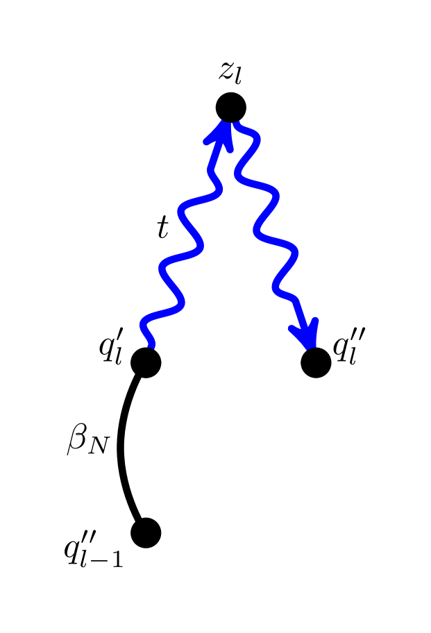
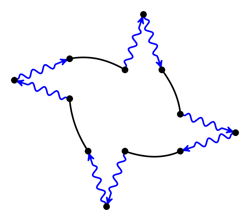
Figure 1: Left: Schematic diagram of the path integral discretization of the block structure $\hat{J}^{(1)}$ (Eq. (6)) used to obtained the generalized Kubo transform in Eq. (9). Blue wavy lines represent the $t$ time propagation. Black lines show the $\beta_{N}$ imaginary time propagation. Right: Schematic diagram of the structure of the Kubo transform time correlation function (Eq. (9)) for $N=4$.

A path integral representation of Eq. (4) can be obtained by inserting identities inside the building blocks $\hat{J}^{(1)}$ in the form (see the schematic representation in Fig. 1)

$$\hat{J}^{(1)} = \int dq^{\prime}_{l}\int dq^{\prime\prime}_{l}\int dz_{l}\ e^{-\beta_{N}\hat{H}}\ket{q^{\prime}_{l}}\bra{q^{\prime}_{l}}e^{i\hat{H}t/\hbar}\ket{z_{l}}\bra{z_{l}}e^{-i\hat{H}t/\hbar}\ket{q^{\prime\prime}_{l}}\bra{q^{\prime\prime}_{l}},$$ (6)

to yield

$$K_{AB}^{[N]}(t) = \frac{1}{Z_{N}}\int d\bm{q^{\prime}}\int d\bm{q^{\prime\prime}}\int d\bm{z}A(\bm{q^{\prime}})B(z_{N})\prod_{l=1}^{N}\langle q^{\prime\prime}_{l-1}|e^{-\beta_{N}\hat{H}}\left|q^{\prime}_{l}\right\rangle$$ (7)

$$\times\left\langle q^{\prime}_{l}\right|e^{i\hat{H}t/\hbar}|z_{l}\rangle\langle z_{l}|e^{-i\hat{H}t/\hbar}\left|q^{\prime\prime}_{l}\right\rangle,$$

where

$$O(\bm{x})=\frac{1}{N}\sum^{N}_{k=1}O(x_{k}),$$ (8)

and $\int d\bm{x}=\int dx_{1}\int dx_{2}\cdots\int dx_{N}$ (with $x_{0}=x_{N}$). Note, however, that due to the cyclic structure of the path integral representation, the operator $\hat{B}$ can be averaged over all $\bm{z}$ coordinates to give an even more symmetric form of the Kubo transform

$$K_{AB}^{[N]}(t) = \frac{1}{Z_{N}}\int d\bm{q^{\prime}}\int d\bm{q^{\prime\prime}}\int d\bm{z}A(\bm{q^{\prime}})B(\bm{z})\prod_{l=1}^{N}\langle q^{\prime\prime}_{l-1}|e^{-\beta_{N}\hat{H}}\left|q^{\prime}_{l}\right\rangle$$ (9)

$$\times\left\langle q^{\prime}_{l}\right|e^{i\hat{H}t/\hbar}|z_{l}\rangle\langle z_{l}|e^{-i\hat{H}t/\hbar}\left|q^{\prime\prime}_{l}\right\rangle.$$

This expression, whose schematic representation is presented in Fig. 1 for $N=4$, represents an exact path integral representation of Eq. (1) in the limit $N\to\infty$ and emphasizes the symmetry with respect to cyclic permutations of the coordinates of the path integral.Hele2015Mats ; Hele2017

In order to make the Matsubara approximation, it is necessary to express Eq. (9) in terms of a phase space average.Wigner1932 To this end, making a change of variables on the Cartesian $\bm{q^{\prime}}$ and $\bm{q^{\prime\prime}}$ variables to sum/difference coordinates

$$q_{l}=\frac{q^{\prime}_{l}+q^{\prime\prime}_{l}}{2}$$ (10)

$$\Delta_{l}=q^{\prime}_{l}-q^{\prime\prime}_{l}$$ (11)

for each value $l=1,...,N$, allows us to re-express Eq. (9) as

$$K_{AB}^{[N]}(t)=\int d\bm{q}\int d\bm{\Delta}\int d\bm{z}A\big{(}\bm{q}+\bm{\Delta}/2\big{)}B(\bm{z})\rho(\bm{q},\bm{\Delta};\beta)G(\bm{q},\bm{\Delta},\bm{z};t),$$ (12)

where we have defined

$$\rho(\bm{q},\bm{\Delta};\beta)=\frac{1}{Z_{N}}\prod_{l=1}^{N}\left\langle q_{l-1}-\frac{\Delta_{l-1}}{2}\right|e^{-\beta_{N}\hat{H}}\left|q_{l}+\frac{\Delta_{l}}{2}\right\rangle,$$ (13)

and

$$G(\bm{q},\bm{\Delta},\bm{z};t)=\prod_{l=1}^{N}\left\langle q_{l}+\frac{\Delta_{l}}{2}\right|e^{i\hat{H}t/\hbar}\Bigl{|}z_{l}\Bigr{\rangle}\Bigl{\langle}z_{l}\Bigr{|}e^{-i\hat{H}t/\hbar}\left|q_{l}-\frac{\Delta_{l}}{2}\right\rangle.$$ (14)

Eq. (12) is known in the literature as the Generalized Kubo Transformed correlation functionJang2016 ; Hele2015Mats . We anticipate that obtaining an expression of this form for multi-time correlation functions would be a key step in the multi-time generalization of Matsubara dynamics (see Secs. III and IV)

Eq. (12) can be recast as a phase space average by inserting identities of the form

$$1=\int d\Delta^{\prime}_{l}\ \delta(\Delta_{l}+\Delta^{\prime}_{l})=(2\pi\hbar)^{-1}\int d\Delta^{\prime}_{l}\int dp_{l}\ e^{ip_{l}(\Delta_{l}+\Delta_{l}^{\prime})/\hbar}$$ (15)

for each $l=1,...,N$, to obtain

$$K_{AB}^{[N]}(t)=\frac{1}{(2\pi\hbar)^{N}}\int d\bm{q}\int d\bm{p}\left[e^{-\beta\hat{H}}\hat{A}\right]_{\overline{N}}(\bm{q},\bm{p})\left[\hat{B}(t)\right]_{N}(\bm{q},\bm{p}),$$ (16)

where

$$\left[e^{-\beta\hat{H}}\hat{A}\right]_{\overline{N}}(\bm{q},\bm{p})=\frac{1}{Z_{N}}\int d\bm{\Delta}A\big{(}\bm{q}+\bm{\Delta}/2\big{)}\prod_{l=1}^{N}\left\langle q_{l-1}-\frac{\Delta_{l-1}}{2}\right|e^{-\beta_{N}\hat{H}}\left|q_{l}+\frac{\Delta_{l}}{2}\right\rangle e^{i\Delta_{l}p_{l}/\hbar},$$ (17)

and

$$\left[\hat{B}(t)\right]_{N}(\bm{q},\bm{p}) = \int d\bm{\Delta}\int d\bm{z}B(\bm{z})\prod_{l=1}^{N}\left\langle q_{l}-\frac{\Delta_{l}}{2}\right|e^{i\hat{H}t/\hbar}\Bigl{|}z_{l}\Bigr{\rangle}$$ (18)

$$\times\Bigl{\langle}z_{l}\Bigr{|}e^{-i\hat{H}t/\hbar}\left|q_{l}+\frac{\Delta_{l}}{2}\right\rangle e^{i\Delta_{l}p_{l}/\hbar}.$$

The generalized Wigner transformWigner1932 in Eq. (17) contains a complex structure that couples different variables together whereas the generalized Wigner transform in Eq. (18) is just a sum of one-dimensional Wigner transformed products. Note that since $\hat{B}$ is just a function of $\hat{x}$ it follows that at time $t=0$

$$\left[\hat{B}(t=0)\right]_{N}(\bm{q},\bm{p})=B(\bm{q}).$$ (19)

To complete the phase space representation of the Kubo transform it is useful to recast Eq. (16) in terms of the quantum Liouvillian instead of the Hamiltonian. By noting that Hillery1984 ; Hele2017

$$\frac{d}{dt}\left[\hat{B}(t)\right]_{N}(\bm{q},\bm{p}) = \hat{L}_{N}\left[\hat{B}(t)\right]_{N}(\bm{q},\bm{p}),$$ (20)

one can formally write the exact correlation function in Eq. (16) as

$$K_{AB}^{[N]}(t)=\frac{1}{(2\pi\hbar)^{N}}\int d\bm{q}\int d\bm{p}\left[e^{-\beta\hat{H}}\hat{A}\right]_{\overline{N}}(\bm{q},\bm{p})e^{\hat{L}_{N}t}B(\bm{q}).$$ (21)

In Eqs. (20) and (21) $\hat{L}_{N}$ represents the Moyal expansion of the quantum Liouvillian of the $N$ blocks as defined byHillery1984 ; Groenewold1946 ; Moyal1949

$$\hat{L}_{N}=\frac{2}{\hbar}\sum_{l=1}^{N}\left[\frac{p_{l}^{2}}{2m}+V(q_{l})\right]\sin\bigg{(}\frac{\hbar}{2}\hat{\Lambda}_{l}\bigg{)}$$ (22)

where

$$\hat{\Lambda}_{l}=\frac{\overleftarrow{\partial}}{\partial p_{l}}\frac{\overrightarrow{\partial}}{\partial q_{l}}-\frac{\overleftarrow{\partial}}{\partial q_{l}}\frac{\overrightarrow{\partial}}{\partial p_{l}},$$ (23)

is known as the Janus operatorLittlejohn1986 and the arrows indicate the direction in which the differential operators are applied, i.e to the left or right. In what follows, it will be convenient to rewrite the Liouvillian more compactly as

$$\hat{L}_{N}=\frac{2}{\hbar}\left[\frac{\bm{p}^{2}}{2m}+U_{N}(\bm{q})\right]\sin\bigg{(}\frac{\hbar}{2}\hat{\Lambda}_{N}\bigg{)},$$ (24)

where

$$U_{N}(\bm{q})=\sum_{l=1}^{N}V(q_{l}),$$ (25)

$$\hat{\Lambda}_{N}=\mathbf{\overleftarrow{\nabla}}_{\bm{p}}\cdot\mathbf{\overrightarrow{\nabla}}_{\bm{q}}-\mathbf{\overleftarrow{\nabla}}_{\bm{q}}\cdot\mathbf{\overrightarrow{\nabla}}_{\bm{p}}$$ (26)

and

$$\mathbf{\nabla}_{\bm{q}}^{T}=\left(\frac{\partial}{\partial q_{1}},\frac{\partial}{\partial q_{2}},\ldots,\frac{\partial}{\partial q_{N}}\right).$$ (27)

The advantage of having the Kubo transformed correlation function expressed as a phase space average in ring polymer coordinates, namely Eq. (21), is that now it is possible to make a coordinate transformation to the normal modes describing the centroid and the fluctuations of the free ring polymer.Richardson2009 ; Markland2008 The normal transformation is defined by the matrix $\underline{\underline{\rm T}}$ with elements

$$T_{lk}=\begin{cases}\sqrt{\frac{1}{N}}&k=0\\ \sqrt{\frac{2}{N}}\sin(2\pi lk/N)&0<k\leq\bar{N}\\ \sqrt{\frac{2}{N}}\cos(2\pi lk/N)&-\bar{N}\leq k<0,\end{cases}$$ (28)

where $\bar{N}=(N-1)/2$ is chosen to be odd for convenience (even N leads to the same resultHele2015Mats ). The normal mode coordinates (denoted as $\bm{Q}$ and $\bm{P}$) are defined by the relations

$$\bm{q}=\sqrt{N}\underline{\underline{\rm T}}\bm{Q}$$ (29)

and

$$\bm{p}=\sqrt{N}\underline{\underline{\rm T}}\bm{P},$$ (30)

where we have included an extra $\sqrt{N}$ factor to ensure that the $\bm{Q}$ converge in the limit $N\to\infty$, giving the centroid for $Q_{0}$. The square roots of the eigenvalues of the matrix defined in Eq. (28) are given by

$$\tilde{\omega}_{k}=\frac{2\sin(k\pi/N)}{\beta_{N}\hbar}.$$ (31)

In these new coordinates Eq. (21) takes the form

$$K_{AB}^{[N]}(t)=\frac{1}{(2\pi\hbar)^{N}}\int d\bm{Q}\int d\bm{P}\left[e^{-\beta\hat{H}}\hat{A}\right]_{\overline{N}}(\bm{Q},\bm{P})e^{\hat{L}_{N}t}B(\bm{Q}),$$ (32)

where $\int d\bm{X}=\int dX_{-\bar{N}}\int dX_{-\bar{N}+1}\cdots\int dX_{\bar{N}-1}\int dX_{\bar{N}}$ and where the Liouvillian in these new coordinates is given by

$$\hat{L}_{N}=\frac{2N}{\hbar}\left[\frac{\bm{P}^{2}}{2m}+\frac{U_{N}(\bm{Q})}{N}\right]\sin\bigg{(}\frac{\hbar}{2N}\hat{\Lambda}_{N}\bigg{)},$$ (33)

with the Janus operator now defined as

$$\hat{\Lambda}_{N}=\overleftarrow{\nabla}_{\bm{P}}\cdot\overrightarrow{\nabla}_{\bm{Q}}-\overleftarrow{\nabla}_{\bm{Q}}\cdot\overrightarrow{\nabla}_{\bm{P}}$$ (34)

Following the notation of T. J. Hele et al.,Hele2015Mats in the above equations and for what follows it is to be understood that all instances of $\bm{Q}$ ($\bm{P}$) inside a function should be interpreted as $\sqrt{N}\underline{\underline{T}}\bm{Q}$ ($\sqrt{N}\underline{\underline{T}}\bm{P}$), i.e. the coordinate transformations defined in Eqs. (29) and (30).

The $M$ lowest frequencies of Eq. (31) in the limit as $N\to\infty$ are known in thermal field theories as the Matsubara modes of distinguishable particles.Matsubara1955 An explicit form for these frequencies exists,

$$\lim_{N\to\infty}\tilde{\omega}_{k}=\omega_{k}=\frac{2\pi k}{\beta\hbar}\ ,\ |k|<\bar{M},$$ (35)

where $\bar{M}=(M-1)/2$. In this limit, the $M$ lowest modes (the Matsubara modes) become Fourier coefficients of the position $q(\tau)=q_{l}$ (with $\tau=\beta_{N}\hbar l$), which means that $q(\tau)$ can be built from a superposition of Matsubara modes as

$$q(\tau)=Q_{0}+\sqrt{2}\sum_{k=1}^{\bar{M}}\sin(\omega_{k}\tau)Q_{k}+\cos(\omega_{k}\tau)Q_{-k}.$$ (36)

The significance of working with the Matsubara modes is that $q(\tau)$ is a smooth and continuous function of the imaginary time variable $\tau$.Hele2015Mats This will not in general be true if $q(\tau)$ is built of both Matsubara and non-Matsubara modes, where the later will give rise to non-smooth (non-Boltzmann) distributions. Note that quite remarkably, at time $t=0$, one can integrate out the non-Matsubara modes of Eq. (32) giving rise to an alternative expression for the Kubo transform in the limit $M\to\infty$, $M<<N$Willatt2018 ; Ceperley1995 ; Chakravarty1997 ; Chakravarty1998 ; Freeman1984

$$K_{AB}^{[M]}(0)=\frac{1}{(2\pi\hbar)^{M}Z_{M}}\int d\bm{Q}\int d\bm{P}e^{-\beta R_{M}(\bm{Q},\bm{P})}A_{M}(\bm{Q})B_{M}(\bm{Q}),$$ (37)

where

$$R_{M}(\bm{Q},\bm{P})=\sum_{n=-\bar{M}}^{\bar{M}}\left(\frac{P^{2}_{n}}{2m}+\frac{m}{2}\omega^{2}_{n}Q^{2}_{n}\right)+U_{M}(\bm{Q}),$$ (38)

$$U_{M}(\bm{Q})=\frac{1}{\beta\hbar}\int_{0}^{\beta\hbar}{\rm d}\tau\ V(q(\tau)),$$ (39)

and

$$Z_{M}=\frac{1}{(2\pi\hbar)^{M}}\int d\bm{Q}\int d\bm{P}e^{-\beta R_{M}(\bm{Q},\bm{P})},$$ (40)

with $A_{M}(\bm{Q})$ and $B_{M}(\bm{Q})$ defined analogously to $U_{M}(\bm{Q})$. This expression is significant since it implies that only smooth Matsubara modes contribute to the Boltzmann average of the Kubo correlation function at time zero. At finite times, unless the potential is harmonic, non-Matsubara modes will couple to the smooth modes due to Eq. (33) and, hence, the distribution would become jagged and detailed balance will not be satisfied. It is worth mentioning that the Janus operator (Eq. (34)) does not couple different normal modes together. It is only through the sine function in Eq. (33) that the Janus operator mixes the modes together in the Liouvillian.

The Matsubara approximation is then to assume that one can neglect the coupling to the non-Matsubara modes for all times and use only the Matsubara modes to describe the time evolution of the system. This is done by neglecting the non-Matsubara mode terms in Eq. (34) which produces the effect of decoupling the non-Matsubara modes from the Matsubara modes in the dynamical evolution. The quantum Liouvillian then reduces to a classical Liouvillian in the Matsubara modes in the limit $N\to\infty$

$$\lim_{N\to\infty}L_{N}\approx\bar{L}_{M}=\sum_{k=-\bar{M}}^{\bar{M}}\frac{P_{k}}{m}\frac{\partial}{\partial Q_{k}}-\frac{1}{N}\frac{\partial U_{N}(\bm{Q})}{\partial Q_{k}}\frac{\partial}{\partial P_{k}},$$ (41)

which happens because in the Matsubara subspace $\hbar$ is replaced by an effective Planck’s constant $\hbar/N$ which in the limit as $N\to\infty$ vanishes. The Matsubara approximation to the Kubo transformed correlation function is then

$$K_{AB}^{[M]}(t)=\lim_{N\to\infty}\frac{1}{(2\pi\hbar)^{N}}\int d\bm{Q}\int d\bm{P}\left[e^{-\beta\hat{H}}\hat{A}\right]_{\overline{N}}(\bm{Q},\bm{P})e^{\bar{L}_{M}t}B(\bm{Q}).$$ (42)

Note that Eq. (42) still depends on the non-Matsubara modes through the potential. However, since these modes are decoupled from the Matsubara modes they can be analytically integrated out to giveHele2015Mats ; footnote_about_delta

$$K_{AB}^{[M]}(t)=\frac{1}{2\pi\hbar Z_{M}}\int d\bm{Q}\int d\bm{P}e^{-\beta H_{M}(\bm{Q},\bm{P})}e^{i\beta\theta_{M}(\bm{Q},\bm{P})}A_{M}(\bm{Q)}e^{L_{M}t}B_{M}(\bm{Q}),$$ (43)

where it is to be understood that all the variables are now of the Matsubara modes only. $L_{M}$ is the classical Liouvillian in the Matsubara subspace (Eq. (41)) but with the Matsubara potential $U_{M}(\bm{Q})$ (defined by Eq. (39)) replacing $U_{N}(\bm{Q})/N$. The Matsubara Hamiltonian is given by

$$H_{M}(\bm{Q},\bm{P})=\sum_{k=-\bar{M}}^{\bar{M}}\frac{P_{k}^{2}}{2m}+U_{M}(\bm{Q}),$$ (44)

and the Matsubara phase, which converts what would be a classical Boltzmann distribution into a quantum one, is

$$\theta_{M}(\bm{Q},\bm{P})=\sum_{k=-\bar{M}}^{\bar{M}}\omega_{k}Q_{-k}P_{k}.$$ (45)

It can be straightforwardly shown that the Matsubara correlation function of Eq. (43) contains all the symmetries of the Kubo transformed correlation function. Furthermore, it can be shown that the classical dynamics generated by the Matsubara Liouvillian preserve both the Matsubara phase and the Boltzmann distribution, which ensures the quantum Boltzmann distribution is conserved during the classical evolution of the Matsubara modes. Matsubara dynamics is also exact in the harmonic limit for any correlation function due to the fact that for this particular potential the non-Matsubara modes do not couple to the Matsubara modes. Matsubara dynamics will perform better than Ring Polymer Molecular Dynamics (RPMD)Craig2004 ; Habershon2008 and Centroid Molecular Dynamics (CMD)Cao1994-2 ; Cao1994-4 ; Jang1999 in general due to the fact that it explicitly includes the fluctuation dynamics that both CMD and RPMD miss. This is to date the most general form of classical Boltzmann preserving dynamics from which it has been shown that RPMD, CMD and the Planetary ModelSmith2015 are in fact approximations of Matsubara dynamicsHele2015 ; Willatt2018 .

III Two-Time Matsubara Dynamics

Having established the key steps of the formulation of single-time Matsubara dynamics, we now present the derivation of the Matsubara approximation for the two-time symmetrized double Kubo transform correlation function. To keep the discussion concise we utilize many of the results from Sec. II.

III.1 Path Integral Discretization of the Symmetrized Double Kubo Transform

We start by defining the symmetrized double Kubo transform as Reichman2000 ; Jung2018

$$K_{ABC}^{sym}(t,t^{\prime})=\frac{1}{Z\beta^{2}}\int_{0}^{\beta}d\lambda\int_{0}^{\beta}d\lambda^{\prime}\bigl{\langle}\hat{T}_{\beta}\hat{A}(-i\hbar\lambda)\hat{B}(-i\hbar\lambda^{\prime}+t)\hat{C}(t^{\prime})\bigr{\rangle},$$ (46)

where $\hat{O}(\tau)=e^{i\hat{H}\tau/\hbar}\hat{O}e^{-i\hat{H}\tau/\hbar}$ and $\hat{T}_{\beta}$ is the imaginary time ordering operator

$$\hat{T}_{\beta}\hat{O}(-i\hbar\lambda)\hat{P}(-i\hbar\lambda^{\prime})=\begin{cases}\hat{O}(-i\hbar\lambda)\hat{P}(-i\hbar\lambda^{\prime})\ \ \ \text{if }\lambda>\lambda^{\prime}\\ \hat{P}(-i\hbar\lambda^{\prime})\hat{O}(-i\hbar\lambda)\ \ \ \text{if }\lambda<\lambda^{\prime}\end{cases}$$ (47)

Here, $t$ and $t^{\prime}$ are taken to be independent time variables. By using the definition of the imaginary time ordering operator and exchanging the integration limits, Eq. (46) can be expressed as

$$K_{ABC}^{sym}(t,t^{\prime})=I_{1}+I_{2}$$ (48)

where

$$I_{1}=\frac{1}{Z\beta^{2}}\int_{0}^{\beta}d\lambda\int_{0}^{\lambda}d\lambda^{\prime}Tr\bigg{[}e^{-(\beta-\lambda)\hat{H}}\hat{A}e^{-(\lambda-\lambda^{\prime})\hat{H}}\hat{B}(t)e^{-\lambda^{\prime}\hat{H}}\hat{C}(t^{\prime})\bigg{]}$$ (49)

and

$$I_{2}=\frac{1}{Z\beta^{2}}\int_{0}^{\beta}d\lambda\int_{0}^{\lambda}d\lambda^{\prime}Tr\bigg{[}e^{-(\beta-\lambda)\hat{H}}\hat{B}(t)e^{-(\lambda-\lambda^{\prime})\hat{H}}\hat{A}e^{-\lambda^{\prime}\hat{H}}\hat{C}(t^{\prime})\bigg{]}.$$ (50)

Note here that $\beta\geq\lambda\geq\lambda^{\prime}\geq 0$, which ensures that there is no backwards imaginary time propagation. The symmetrized Double Kubo transform is a real function of time that shares the formal properties and symmetries with classical two-time correlation functions (see Appendix of Ref. 44) and has recently been related to the second-order response function of nonlinear spectroscopy.Jung2018

Following the ideas of the previous section, we discretize the iterated integrals and make the expression more symmetric by inserting $N-1$ identities of the form

$$\hat{1}=e^{i\hat{H}t/\hbar}e^{-i\hat{H}t/\hbar}e^{i\hat{H}t^{\prime}/\hbar}e^{-i\hat{H}t^{\prime}/\hbar},$$ (51)

to obtain

$$I_{1} = \frac{1}{Z_{N}N^{2}}\sum^{N}_{k=1}\sum^{k}_{l=1}Tr\bigg{[}\bigg{(}e^{-\beta_{N}\hat{H}}e^{i\hat{H}t/\hbar}e^{-i\hat{H}t/\hbar}e^{i\hat{H}t^{\prime}/\hbar}e^{-i\hat{H}t^{\prime}/\hbar}\bigg{)}^{N-k-1}$$ (52)

$$\times e^{-\beta_{N}\hat{H}}\hat{A}e^{i\hat{H}t/\hbar}e^{-i\hat{H}t/\hbar}e^{i\hat{H}t^{\prime}/\hbar}e^{-i\hat{H}t^{\prime}/\hbar}\bigg{(}e^{-\beta_{N}\hat{H}}e^{i\hat{H}t/\hbar}e^{-i\hat{H}t/\hbar}e^{i\hat{H}t^{\prime}/\hbar}e^{-i\hat{H}t^{\prime}/\hbar}\bigg{)}^{k-l-1}$$

$$\times e^{-\beta_{N}\hat{H}}e^{i\hat{H}t/\hbar}\hat{B}e^{-i\hat{H}t/\hbar}e^{i\hat{H}t^{\prime}/\hbar}e^{-i\hat{H}t^{\prime}/\hbar}\bigg{(}e^{-\beta_{N}\hat{H}}e^{i\hat{H}t/\hbar}e^{-i\hat{H}t/\hbar}e^{i\hat{H}t^{\prime}/\hbar}e^{-i\hat{H}t^{\prime}/\hbar}\bigg{)}^{l-1}$$

$$\times e^{-\beta_{N}\hat{H}}e^{i\hat{H}t/\hbar}e^{-i\hat{H}t/\hbar}e^{i\hat{H}t^{\prime}/\hbar}\hat{C}e^{-i\hat{H}t^{\prime}/\hbar}\bigg{]}$$

and

$$I_{2} = \frac{1}{Z_{N}N^{2}}\sum^{N}_{k=1}\sum^{k}_{l=1}Tr\bigg{[}\bigg{(}e^{-\beta_{N}\hat{H}}e^{i\hat{H}t/\hbar}e^{-i\hat{H}t/\hbar}e^{i\hat{H}t^{\prime}/\hbar}e^{-i\hat{H}t^{\prime}/\hbar}\bigg{)}^{N-k-1}$$ (53)

$$\times e^{-\beta_{N}\hat{H}}e^{i\hat{H}t/\hbar}\hat{B}e^{-i\hat{H}t/\hbar}e^{i\hat{H}t^{\prime}/\hbar}e^{-i\hat{H}t^{\prime}/\hbar}\bigg{(}e^{-\beta_{N}\hat{H}}e^{i\hat{H}t/\hbar}e^{-i\hat{H}t/\hbar}e^{i\hat{H}t^{\prime}/\hbar}e^{-i\hat{H}t^{\prime}/\hbar}\bigg{)}^{k-l-1}$$

$$\times e^{-\beta_{N}\hat{H}}\hat{A}e^{i\hat{H}t/\hbar}e^{-i\hat{H}t/\hbar}e^{i\hat{H}t^{\prime}/\hbar}e^{-i\hat{H}t^{\prime}/\hbar}\bigg{(}e^{-\beta_{N}\hat{H}}e^{i\hat{H}t/\hbar}e^{-i\hat{H}t/\hbar}e^{i\hat{H}t^{\prime}/\hbar}e^{-i\hat{H}t^{\prime}/\hbar}\bigg{)}^{l-1}$$

$$\times e^{-\beta_{N}\hat{H}}e^{i\hat{H}t/\hbar}e^{-i\hat{H}t/\hbar}e^{i\hat{H}t^{\prime}/\hbar}\hat{C}e^{-i\hat{H}t^{\prime}/\hbar}\bigg{]}.$$

The structure of Eqs. (52) and (53) suggests that the interpretation of the double Kubo transforms can be cast in terms of a new block structure of the form $\hat{J}^{(2)}=e^{-\beta\hat{H}}e^{i\hat{H}t/\hbar}e^{-i\hat{H}t/\hbar}e^{i\hat{H}t^{\prime}/\hbar}e^{-i\hat{H}t^{\prime}/\hbar}$ with the operators $\hat{A}$ and $\hat{B}$ evaluated in different blocks depending of the sum indexes. Note, however, that in Eq. (52) the operator $\hat{A}$ is evaluated over all the blocks whereas the operator $\hat{B}$ is evaluated only at particular blocks (constrained by the inner sum index); in Eq. (53) the opposite behavior is found, i.e. $\hat{B}$ is evaluated over all the blocks whereas $\hat{A}$ is constrained at particular blocks. This is a consequence of the imaginary time ordering found in Eqs. (49) and (50). However, since the underling block structure is the same for both $I_{1}$ and $I_{2}$ (i.e. the block structure $\hat{J}^{(2)}$ is common to both traces), the sum of $I_{1}$ and $I_{2}$ allows the evaluation of both $\hat{A}$ and $\hat{B}$ over all the blocks. This is vital for obtaining a symmetric form of the Kubo transform and will be crucial for constructing the multi-time generalization of Matsubara dynamics (see section IV).

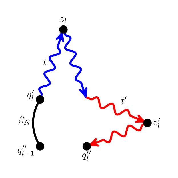
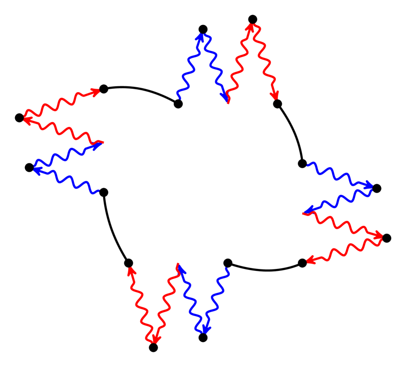
Figure 2: Left: Schematic diagram of the path integral discretization of the block structure $\hat{J}^{(2)}$ used to obtained the generalized symmetrized double Kubo transform in Eq. (56). Blue wavy lines show the $t$ propagation. Red wavy lines show the $t^{\prime}$ propagation. Black lines show the $\beta_{N}$ propagation. Note that there is no identity inserted between the forward $t$ evolution and the backward $t^{\prime}$ evolution. Right: Schematic diagram of the structure of the generalized symmetrized double Kubo transform time correlation function (Eq. (56))

To obtain a path integral representation of the double Kubo transform, we path integral discretize the building blocks $\hat{J}^{(2)}$ in the form (see Fig. 2 for an schematic representation)

$$\hat{J}^{(2)} = \int dq^{\prime}_{l}\int dq^{\prime\prime}_{l}\int dz_{l}\int dz^{\prime}_{l}\ e^{-\beta_{N}\hat{H}}\ket{q^{\prime}_{l}}\bra{q^{\prime}_{l}}e^{i\hat{H}t/\hbar}\ket{z_{l}}\bra{z_{l}}e^{-i\hat{H}t/\hbar}e^{i\hat{H}t^{\prime}/\hbar}\ket{z^{\prime}_{l}}\bra{z^{\prime}_{l}}e^{-i\hat{H}t^{\prime}/\hbar}\ket{q^{\prime\prime}_{l}}\bra{q^{\prime\prime}_{l}}.$$ (54)

and add Eqs. (52) and (53) to obtain

$$K_{ABC}^{sym,[N]}(t,t^{\prime}) = \frac{1}{Z_{N}}\int d\bm{q^{\prime}}\int d\bm{q^{\prime\prime}}\int d\bm{z}\int d\bm{z^{\prime}}A(\bm{q^{\prime}})B(\bm{z})C(\bm{z^{\prime}})$$ (55)

$$\times\prod_{l=1}^{N}\left\langle q^{\prime\prime}_{l-1}\right|e^{-\beta_{N}\hat{H}}\left|q^{\prime}_{l}\right\rangle\left\langle q^{\prime}_{l}\right|e^{i\hat{H}t/\hbar}\Bigl{|}z_{l}\Bigr{\rangle}$$

$$\times\Bigl{\langle}z_{l}\Bigr{|}e^{-i\hat{H}t/\hbar}e^{i\hat{H}t^{\prime}/\hbar}\left|z_{l}^{{}^{\prime}}\right\rangle\left\langle z_{l}^{{}^{\prime}}\right|e^{-i\hat{H}t^{\prime}/\hbar}\left|q^{\prime\prime}_{l}\right\rangle.$$

An schematic diagram of this expression for $N=4$ is shown in Fig. 2 and highlights the symmetry of the symmetrized Double Kubo transform.

By making the change of variables from Cartesian coordinates to the sum/difference coordinates of Eqs. (10) and (11), we can re-express Eq. (55) as

$$K_{ABC}^{sym,[N]}(t,t^{\prime})=\int d\bm{q}\int d\bm{\Delta}\int d\bm{z}\int d\bm{z^{\prime}}A(\bm{q}+\bm{\Delta}/2)B(\bm{z})C(\bm{z^{\prime}})\rho(\bm{q},\bm{\Delta};\beta)G(\bm{q},\bm{\Delta},\bm{z},\bm{z^{\prime}};t,t^{\prime}),$$ (56)

where $\rho(\bm{q},\bm{\Delta};\beta)$ is defined in Eq. (13) and

$$G(\bm{q},\bm{\Delta},\bm{z},\bm{z}^{\prime};t,t^{\prime})=\prod_{l=1}^{N}\left\langle q_{l}+\frac{\Delta_{l}}{2}\right|e^{i\hat{H}t/\hbar}\Bigl{|}z_{l}\Bigr{\rangle}\Bigl{\langle}z_{l}\Bigr{|}e^{-i\hat{H}t/\hbar}e^{i\hat{H}t^{\prime}/\hbar}\left|z_{l}^{{}^{\prime}}\right\rangle\left\langle z_{l}^{{}^{\prime}}\right|e^{-i\hat{H}t^{\prime}/\hbar}\left|q_{l}-\frac{\Delta_{l}}{2}\right\rangle.$$ (57)

Eq. (56), which we term the Generalized Double Kubo Transformed correlation function, corresponds to an exact path integral representation of the symmetrized double Kubo transform and represents the first important result of this paper. To the best of our knowledge, this is the first time that an expression that emphasizes the symmetry with respect to cyclic permutations of the coordinates of the path integral for the symmetrized double Kubo transform has been presented.

III.2 Phase space representation

A phase space representation of the Generalized Double Kubo Transform Eq. (56) can be obtained by inserting Dirac delta identities of the form of Eq. (15) to arrive at:

$$K_{ABC}^{sym,[N]}(t,t^{\prime})=\frac{1}{(2\pi\hbar)^{N}}\int d\bm{q}\int d\bm{p}\left[e^{\beta\hat{H}}\hat{A}\right]_{\overline{N}}(\bm{q},\bm{p})\left[\hat{B}(t)\hat{C}(t^{\prime})\right]_{N}(\bm{q},\bm{p}),$$ (58)

where $\left[e^{\beta\hat{H}}\hat{A}\right]_{\overline{N}}(\bm{q},\bm{p})$ has been defined in Eq. (17) and

$$\left[\hat{B}(t)\hat{C}(t^{\prime})\right]_{N}(\bm{q},\bm{p}) = \int d\bm{\Delta}\int d\bm{z}\int d\bm{z^{\prime}}B(\bm{z})C(\bm{z^{\prime}})\prod_{l=1}^{N}\left\langle q_{l}-\frac{\Delta_{l}}{2}\right|e^{i\hat{H}t/\hbar}\Bigl{|}z_{l}\Bigr{\rangle}$$ (59)

$$\times\Bigl{\langle}z_{l}\Bigr{|}e^{-i\hat{H}t/\hbar}e^{i\hat{H}t^{\prime}/\hbar}\left|z_{l}^{{}^{\prime}}\right\rangle\left\langle z_{l}^{{}^{\prime}}\right|e^{-i\hat{H}t^{\prime}/\hbar}\left|q_{l}+\frac{\Delta_{l}}{2}\right\rangle e^{i\Delta_{l}p_{l}/\hbar}.$$

The structure of the two-time Wigner transform in Eq. (59) involves a double sum over products of one-dimensional Wigner transforms. However, with the use of the Moyal product,Hillery1984 ; star_product which replaces a Wigner transformed product with a product of Wigner transforms, it can be recast in the more compact form (see Appendix A):

$$\left[\hat{B}(t)\hat{C}(t^{\prime})\right]_{N}(\bm{q},\bm{p})=\left[\hat{B}(t)\right]_{N}(\bm{q},\bm{p})e^{-i\hbar\hat{\Lambda}_{N}/2}\left[\hat{C}(t^{\prime})\right]_{N}(\bm{q},\bm{p}),$$ (60)

with $\left[\hat{{\cal O}}(t)\right]_{N}(\bm{q},\bm{p})$ defined in Eq. (18) and the Janus operator $\hat{\Lambda}_{N}$ defined in Eq. (26). Since $\hat{A}$ and $\hat{B}$ only depend on position, at $t=t^{\prime}=0$ it follows that:

$$\left[\hat{B}(0)\hat{C}(0)\right]_{N}(\bm{q},\bm{p})=B(\bm{q})C(\bm{q}).$$ (61)

Noting that due to the identity in Eq. (60) and the fact that $t$ and $t^{\prime}$ are independent variables it holds that

$$\frac{d^{n}}{dt^{n}}\frac{d^{m}}{dt^{\prime m}}\left[\hat{B}(t)\hat{C}(t^{\prime})\right]_{N}(\bm{q},\bm{p})=(\hat{L}_{N})^{n}\left[\hat{B}(t)\right]_{N}(\bm{q},\bm{p})e^{-i\hbar\hat{\Lambda}_{N}/2}(\hat{L}_{N})^{m}\left[\hat{C}(t^{\prime})\right]_{N}(\bm{q},\bm{p}),$$ (62)

where $\hat{L}_{N}$ is the Liouvillian defined in Eq. (22), Eq. (58) can be recast in terms of a phase space representation as:

$$K_{ABC}^{sym,[N]}(t,t^{\prime})=\frac{1}{(2\pi\hbar)^{N}}\int d\bm{q}\int d\bm{p}\left[e^{\beta\hat{H}}\hat{A}\right]_{\overline{N}}(\bm{q},\bm{p})e^{\hat{L}_{N}t}B(\bm{q})e^{-i\hbar\hat{\Lambda}_{N}/2}e^{\hat{L}_{N}t^{\prime}}C(\bm{q}).$$ (63)

Eq. (63) corresponds to an exact ring polymer phase average representation of the symmetrized double Kubo transformed correlation and, to the best of our knowledge, represents a novel expression. Note that if not for the Moyal product term, $e^{-i\hbar\hat{\Lambda}_{N}/2}$, the time evolution of the double Kubo transform would involve the action of the (exact) Liouvillian operator $\hat{L}_{N}$ on the observables $\hat{B}$ and $\hat{C}$ for times $t$ and $t^{\prime}$ independently. The effect of the Moyal term is then to couple trajectories at different times with one another, which is a consequence of the interference nature of quantum mechanics.Mukamel1996

III.3 Two-Time Matsubara Dynamics Approximation

It is straightforward to recast Eq. (63) in terms of normal mode coordinates by applying the transformation in Eq. (28) to obtain

$$K_{ABC}^{sym,[N]}(t,t^{\prime}) = \frac{1}{(2\pi\hbar)^{N}Z_{N}}\int d\bm{Q}\int d\bm{P}\left[e^{\beta\hat{H}}\hat{A}\right]_{\overline{N}}(\bm{Q},\bm{P})$$ (64)

$$\times e^{\hat{L}_{N}t}B(\bm{Q})e^{-i\hbar\hat{\Lambda}_{N}/2N}e^{\hat{L}_{N}t^{\prime}}C(\bm{Q})$$

Note that since in the normal coordinates each derivative with respect to $Q_{k}$ ($P_{k}$) brings a factor of $N^{-1/2}$, the Moyal product term in Eq. (64) has an effective Planck constant of $\hbar/N$.

Note that at time $t=t^{\prime}=0$, where Eq. (61) holds, the same integration of non-Matsubara modes as in Eq. (37) can be done,Hele2015Mats resulting in an expression that only involves Matsubara modes. Following ideas from the single time Matsubara dynamics one can make the same approximation of decoupling the dynamical evolution of the non-Matsubara modes from the Matsubara modes by neglecting the non-Matsubara terms in the Janus operator (in the limit as $N\to\infty$ such that $M\ll N$). Note that this approximation has two consequences in Eq. (64): first, just as in the single-time approximation, the Liouvillian $\hat{L}_{N}$ is replaced by the classical Matsubara Liouvillian $\bar{L}_{M}$; second, due to the effective Planck constant $\hbar/N$ in the Moyal product, $e^{-i\hbar\hat{\Lambda}_{N}/2N}$ is forced to unity in the limit $N\to\infty$. Hence, under the Matsubara approximation, Eq. (64) becomes

$$K_{ABC}^{sym,[N]}(t,t^{\prime}) = \lim_{N\to\infty}\frac{1}{(2\pi\hbar)^{N}Z_{N}}\int d\bm{Q}\int d\bm{P}\left[e^{\beta\hat{H}}\hat{A}\right]_{\overline{N}}(\bm{Q},\bm{P})$$ (65)

$$\times e^{\bar{L}_{M}t}B(\bm{Q})e^{\bar{L}_{M}t^{\prime}}C(\bm{Q}).$$

Note that, just as in the original Matsubara derivation, we have not used the assumption that $\hbar\to 0$ to reach to this classical expression, but rather used the fact that in the Matsubara subspace linearization of the dynamics arises naturally in the limit as $N\to\infty$ (due to the effective Planck constant $\hbar/N$ going to zero).

Eq. (65) still depends on the non-Matsubara modes through the potential term in $\bar{L}_{M}$. However, since the conjugate momenta of the non-Matsubara modes are not present in the Liouvillian nor in $A(\bm{Q})$, $B(\bm{Q})$ or $C(\bm{Q})$ one can integrate out the non-Matsubara modes, just as in the single-time Matsubara formulation, to obtain

$$K_{ABC}^{sym,[M]}(t,t^{\prime}) = \frac{1}{2\pi\hbar Z_{M}}\int d\bm{Q}\int d\bm{P}e^{-\beta H_{M}(\bm{Q},\bm{P})}e^{i\beta\theta_{M}(\bm{Q},\bm{P})}$$ (66)

$$\times A_{M}(\bm{Q})e^{L_{M}t}B_{M}(\bm{Q})e^{L_{M}t^{\prime}}C_{M}(\bm{Q}),$$

where it is understood that the integration is performed over only the Matsubara modes. This expression represents the Matsubara approximation to the symmetrized double Kubo transform and is another major result of the paper. Since the dynamics of both $B(\bm{Q})$ and $C(\bm{Q})$ are generated from the classical Matsubara Liouvillian, which conserves both the Matsubara Hamiltonian and phase factor, it follows that Eq. (66) satisfies detailed balance and thus preserves the quantum Boltzmann distribution. Matsubara dynamics is still exact in the harmonic limit for any two-time correlation function and contains all the same symmetries as the exact double Kubo Transform correlation function. In Appendix B we present a numerical demonstration of the convergence of Eq. (66) for a model system.

At time $t=t^{\prime}=0$ one can obtain an alternative expression to Eq. (66). Following Ref. 38, one can perform the same analytic continuation of the phase factor to obtain

$$K_{ABC}^{sym,[M]}(0,0)=\frac{1}{2\pi\hbar Z_{M}}\int d\bm{Q}\int d\bm{P}e^{-\beta R_{M}(\bm{Q},\bm{P})}A_{M}(\bm{Q})B_{M}(\bm{Q})C_{M}(\bm{Q}),$$ (67)

where $R_{M}(\bm{Q},\bm{P})$ is the ring polymer Hamiltonian in normal mode coordinates defined in Eq. (38). This expression represents an exact (smoothed) path integral Fourier representation of the statistics of three operators and is equivalent (in the limit of large $M$) to previously derived expressions.Reichman2000 ; Jung2018

IV Generalization to Multi-time

Following the derivation of the previous sections, it is possible to perform a generalization of the Matsubara dynamics approximation to any order of the symmetrized Kubo transformed multi-time correlation function. In general, the fully symmetrized $n$-th order Kubo transform is given by

$$K^{sym}(\bm{t})\equiv\frac{1}{Z\beta^{n}}\int_{0}^{\beta}d\lambda_{1}\int_{0}^{\beta}d\lambda_{2}\cdot\cdot\cdot\int_{0}^{\beta}d\lambda_{n-1}\int_{0}^{\beta}d\lambda_{n}$$

$$\times\bigl{\langle}\hat{T}_{\beta}A_{0}(-i\hbar\lambda_{1})A_{1}(-i\hbar\lambda_{2}+t_{1})\cdot\cdot\cdot A_{n-1}(-i\hbar\lambda_{n}+t_{n-1})A_{n}(t_{n})\bigr{\rangle},$$ (68)

where $\bm{t}=(t_{1},t_{2},\cdots,t_{n})$ and $\hat{T}_{\beta}$ is a generalization of Eq. (47). Note that the single Kubo transform (Eq. (1)) and the symmetrized Double Kubo transform (Eq. (46)) are special cases of this definition (for $n=1$ and $n=2$, respectively).

By expanding the time ordering operator $\hat{T}_{\beta}$, using properties of the trace and exchanging the integration limits, Eq. (68) can be expressed as a sum of $n!$ terms of the form

$$K^{sym}(\bm{t})=\sum_{j=1}^{n!}I_{j}(\bm{t})$$ (69)

where $I_{j}(\bm{t})$ represents an ordered Kubo transformation with $\beta\geq\lambda_{1}\geq\lambda_{2}\geq\cdots\lambda_{n}\geq 0$. An example of what one of these terms looks like is

$$I_{1} = \frac{1}{Z\beta^{n}}\int_{0}^{\beta}d\lambda_{1}\int_{0}^{\lambda_{1}}d\lambda_{2}\cdots\int_{0}^{\lambda_{n-1}}d\lambda_{n}$$ (70)

$$Tr\bigg{[}e^{-(\beta-\lambda_{1})\hat{H}}\hat{A}_{0}e^{-(\lambda_{1}-\lambda_{2})\hat{H}}\hat{A}_{1}(t_{1})\cdots e^{-\lambda_{n}\hat{H}}\hat{A}_{n}(t_{n})\bigg{]}.$$

Note that $n!$ accounts for all the possible permutations of the $n$ operators $\{A_{0},A_{1},\cdots,A_{n-1}\}$ inside the integral. For the $n=2$ case, the $2!=2$ terms in Eq. (69) are given by Eqs. (49) and (50).

Generalizing ideas from the previous section, one can discretize the integrals and insert $N-1$ identities of the form

$$\hat{1}=e^{i\hat{H}t_{1}/\hbar}e^{-i\hat{H}t_{1}/\hbar}e^{i\hat{H}t_{2}/\hbar}e^{-i\hat{H}t_{2}/\hbar}\cdots e^{i\hat{H}t_{n}/\hbar}e^{-i\hat{H}t_{n}/\hbar},$$ (71)

to obtain for each $I_{j}$ a symmetric expression that involves repeating blocks of the form

$$\hat{J}^{(n)}=e^{-\beta\hat{H}}e^{i\hat{H}t_{1}/\hbar}e^{-i\hat{H}t_{1}/\hbar}e^{i\hat{H}t_{2}/\hbar}e^{-i\hat{H}t_{2}/\hbar}\cdots e^{i\hat{H}t_{n}/\hbar}e^{-i\hat{H}t_{n}/\hbar}$$ (72)

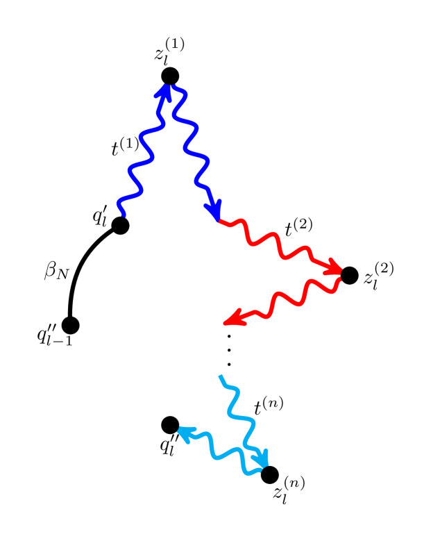
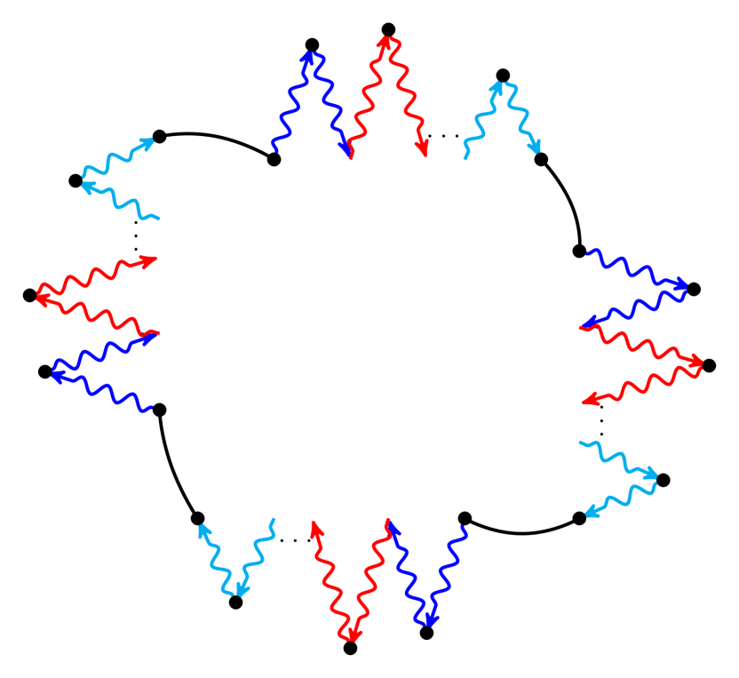
Figure 3: Left: Schematic diagram of the path integral discretization of the block structure $\hat{J}^{(n)}$ (Eq. (73)) used to obtained Eq. (74). Right: Schematic diagram of the structure of the general multi-time symmetrized Kubo transform time correlation function (Eq. (74)) for $N=4$.

with the operators $\{A_{0},A_{1},\cdots,A_{n-1}\}$ intercalated in a particular order and evaluated at a particular block. Following the same logic as in the two-time case, and noting that the underling building block structure is the same for all $I_{j}$ terms, the sum of the $n!$ terms allows to evaluate all the $A_{n}$ operators over all the blocks. Hence, by path integral discretizing the building blocks in the form (see Fig. 3)

$$\hat{J}^{(n)} = \int dq^{\prime}_{l}\int dq^{\prime\prime}_{l}\int dz^{(1)}_{l}\int dz^{(2)}_{l}\cdots\int dz^{(n)}_{l}$$ (73)

$$e^{-\beta_{N}\hat{H}}\ket{q^{\prime}_{l}}\bra{q^{\prime}_{l}}e^{i\hat{H}t_{1}/\hbar}\ket{z^{(1)}_{l}}\bra{z^{(1)}_{l}}e^{-i\hat{H}t_{1}/\hbar}e^{i\hat{H}t_{2}/\hbar}\ket{z^{(2)}_{l}}\cdots$$

$$\bra{z^{(n-1)}_{l}}e^{-i\hat{H}t_{n-1}/\hbar}e^{i\hat{H}t_{n}/\hbar}\ket{z^{(n)}_{l}}\bra{z^{(n)}_{l}}e^{-i\hat{H}t_{n}/\hbar}\ket{q^{\prime\prime}_{l}}\bra{q^{\prime\prime}_{l}}$$

and performing the change of variables from the $\bm{q^{\prime}}$ and $\bm{q^{\prime\prime}}$ Cartesian coordinates to $\bm{q}$ and $\bm{\Delta}$ sum/difference coordinates, the fully symmetrized $n$-th order Kubo transform Eq. (68) can be cast as

$$K^{sym,[N]}(\bm{t}) = \int d\bm{q}\int d\bm{\Delta}\int d\bm{z^{(1)}}\int d\bm{z^{(2)}}\cdots\int d\bm{z^{(n)}}$$ (74)

$$A_{0}(\bm{q}+\bm{\Delta}/2)A_{1}(\bm{z^{(1)}})A_{2}(\bm{z^{(2)}})\cdots A_{n}(\bm{z^{(n)}})\rho(\bm{q},\bm{\Delta};\beta)$$

$$G(\bm{q},\bm{\Delta},\bm{z^{(1)}},\bm{z^{(2)}},\cdots,\bm{z^{(n)}};\bm{t}),$$

where $\rho(\bm{q},\bm{\Delta};\beta)$ is defined in Eq. (13) and $G(\bm{q},\bm{\Delta},\bm{z},\bm{z^{(1)}},\cdots,\bm{z^{(n)}};\bm{t})$ is a multi-time generalization of Eq. (57). Eq. (74) represents the complete multi-time extension of the Generalized symmetrized Kubo transform correlation function and corresponds to an exact path integral representation of Eq. (68). An schematic representation of this expression for $N=4$ is presented in Fig. 3.

Inserting delta function identities allows one to re-express Eq. (74) as a phase space average of the form

$$K^{sym,[N]}(\bm{t}) = \frac{1}{(2\pi\hbar)^{N}}\int d\bm{q}\int d\bm{p}\left[e^{\beta\hat{H}}\hat{A}_{0}\right]_{\overline{N}}(\bm{q},\bm{p})\left[\hat{A}_{1}(t_{1})\hat{A}_{2}(t_{2})\cdots\hat{A}_{n}(t_{n})\right]_{N}(\bm{q},\bm{p}),$$ (75)

with $\left[\hat{A}_{1}(t_{1})\hat{A}_{2}(t_{2})\cdots\hat{A}_{n}(t_{n})\right]_{N}(\bm{q},\bm{p})$ being the multi-time generalization of Eq. (59). Using a generalization of the derivation presented in Appendix A

$$\left[\hat{A}_{1}(t_{1})\hat{A}_{2}(t_{2})\cdots\hat{A}_{n}(t_{n})\right]_{N} = \left[\hat{A}_{1}(t_{1})\right]_{N}e^{-i\hbar\hat{\Lambda}_{N}/2}\left[\hat{A}_{2}(t_{2})\right]_{N}e^{-i\hbar\hat{\Lambda}_{N}/2}\cdots$$ (76)

$$\left[\hat{A}_{n-1}(t_{n-1})\right]_{N}e^{-i\hbar\hat{\Lambda}_{N}/2}\left[\hat{A}_{n}(t_{n})\right]_{N},$$

and the fact that all the times are independent of one another, the $N$ bead phase space representation of Eq. (68) is given by

$$K^{sym,[N]}(\bm{t}) = \frac{1}{(2\pi\hbar)^{N}}\int d\bm{q}\int d\bm{p}\left[e^{\beta\hat{H}}\hat{A}_{0}\right]_{\overline{N}}(\bm{q},\bm{p})e^{\hat{L}_{N}t_{1}}A_{1}(\bm{q})e^{-i\hbar\hat{\Lambda}_{N}/2}$$ (77)

$$\times e^{\hat{L}_{N}t_{2}}A_{2}(\bm{q})\cdot\cdot\cdot e^{\hat{L}_{N}t_{n-1}}A_{n-1}(\bm{q})e^{-i\hbar\hat{\Lambda}_{N}/2}e^{\hat{L}_{N}t_{n}}A_{n}(\bm{q}).$$

The Matsubara approximation to Eq. (77) can be obtained by transforming to normal modes, taking the limit $N\to\infty$ and neglecting the non-Matsubara modes from the Janus operator $\hat{\Lambda}_{N}$ to yield

$$K^{sym,[M]}(\bm{t}) = \frac{1}{2\pi\hbar Z_{M}}\int d\bm{Q}\int d\bm{P}\ e^{-\beta H(\bm{Q},\bm{P})}e^{i\beta\theta(\bm{Q},\bm{P})}$$ (78)

$$\times A_{0}(\bm{Q})e^{L_{M}t_{1}}A_{1}(\bm{Q})e^{L_{M}t_{2}}A_{2}(\bm{Q})\cdots$$

$$\times e^{L_{M}t_{n-1}}A_{n-1}(\bm{Q})e^{L_{M}t_{n}}A_{n}(\bm{Q}).$$

The multi-time generalization of Matsubara dynamics is, just as the single-time counterpart, a classical-like approximation to the Kubo transformed quantum multi-time correlation function that preserves the Boltzmann distribution. Eq. (78) is the most general form of Matsubara dynamics under the Born-Oppenheimer approximation from which it can be seen that the single-time formulation is just a special case of it.

V Conclusions and Future Work

In the present work we have presented a multi-time generalization of Matsubara dynamicsHele2015Mats for the calculation of multi-time correlation functions. The theory is based on the decoupling of the non-Matsubara modes from the Matsubara modes in the dynamical evolution and provides a general consistent way of obtaining classical dynamics from quantum dynamics while preserving the quantum Boltzmann statistics. Any practical approximation that has been developed for the single-time caseWillatt2018 ; Craig2004 ; Cao1994-4 ; Trenins2018 should be straightforwardly applicable.

The multi-time generalization of Matsubara dynamics approximates multi-time fully symmetrized Kubo transformed correlation functions. The symmetrized nature of these functions guarantees they are always real-valued. However, for general multi-time correlation functions, other possible Kubo correlation functions exist. For example, we have shown how the second order response function of non-linear spectroscopy can be expressed in terms of symmetrized and asymmetric double Kubo transform, the latter being a purely imaginary function of time.Jung2018 This raises the question if similar Boltzmann conserving classical dynamics approximations to the one presented here can be developed to more general Kubo transformed correlation functions. Future work in this are will be needed to address this question.

Besides deriving the multi-time formulation of Matsubara dynamics, which is the main purpose of the work, the derivation presented here also provides an exact expression for the evaluation of the multi-time symmetrized Kubo transform, both in path integral form (Eq. (74)) or as a phase space average (Eq. (77)). Although these expressions are impractical for the calculation of multi-time correlations functions for condensed phases systems, they might serve as starting points for the development of other semi-classical approximations. Work in this direction is currently underway.

Appendix A Proof of Eq. (60)

To prove that Eq. (60) holds, it is useful to re-express Eq. (59), by noting that $N-1$ of the forward-backward propagations are identities, as

$$\left[\hat{B}(t)\hat{C}(t^{\prime})\right]_{N}(\bm{q},\bm{p}) = \sum_{j=1}^{N}\left[\hat{B}(t)\hat{C}(t^{\prime})\right]_{W}(q_{j},p_{j})$$ (79)

$$+ \sum_{\begin{subarray}{c}j,k=1\\ j\neq k\end{subarray}}^{N}\left[\hat{B}(t)\right]_{W}(q_{j},p_{j})\left[\hat{C}(t^{\prime})\right]_{W}(q_{k},p_{k})$$

where $\left[\hat{O}\right]_{W}$ defines the Wigner transform of operator $\hat{O}$ as

$$\left[\hat{O}\right]_{W}(q,p)=\int d\Delta e^{ip\Delta/\hbar}\bra{q-\Delta/2}\hat{O}\ket{q+\Delta/2}.$$ (80)

Noting that the Wigner transform of a product is given byHillery1984

$$\left[\hat{O_{1}}\hat{O_{2}}\right]_{W}(q,p)=\left[\hat{O_{1}}\right]_{W}(q,p)e^{-i\hat{\Lambda}\hbar/2}\left[\hat{O_{2}}\right]_{W}(q,p)$$ (81)

where $\hat{\Lambda}$ is the Janus operator (see Eq. 23), the terms in the first sum can be further re-expressed as

$$\left[\hat{B}(t)\hat{C}(t^{\prime})\right]_{N}(\bm{q},\bm{p}) = \sum_{j=1}^{N}\left[\hat{B}(t)\right]_{W}(q_{j},p_{j})e^{-i\hat{\Lambda}_{j}\hbar/2}\left[\hat{C}(t^{\prime})\right]_{W}(q_{j},p_{j})$$ (82)

$$+ \sum_{\begin{subarray}{c}j,k=1\\ j\neq k\end{subarray}}^{N}\left[\hat{B}(t)\right]_{W}(q_{j},p_{j})\left[\hat{C}(t^{\prime})\right]_{W}(q_{k},p_{k}).$$

Using the definition of the Janus operator $\hat{\Lambda}_{j}$ and noting that the leading order of an exponential is 1, the previous expression can be cast as

$$\left[\hat{B}(t)\hat{C}(t^{\prime})\right]_{N}(\bm{q},\bm{p}) = \sum_{j,k=1}^{N}\left[\hat{B}(t)\right]_{W}(q_{j},p_{j})e^{-i\hat{\Lambda}_{j}\hbar/2}\left[\hat{C}(t^{\prime})\right]_{W}(q_{k},p_{k}).$$ (83)

Noting that mixed derivatives inside the sum are zero, namely

$$\left[\hat{B}(t)\right]_{W}(q_{j},p_{j})e^{-i\hat{\Lambda}_{j}\hbar/2}=\left[\hat{B}(t)\right]_{W}(q_{j},p_{j})e^{-i\sum_{l=1}^{N}\hat{\Lambda}_{l}\hbar/2}$$ (84)

the previous equation can be recast as

$$\left[\hat{B}(t)\hat{C}(t^{\prime})\right]_{N}(\bm{q},\bm{p}) = \left(\sum_{j=1}^{N}\left[\hat{B}(t)\right]_{W}(q_{j},p_{j})\right)e^{-i\sum_{l=1}^{N}\hat{\Lambda}_{l}\hbar/2}\left(\sum_{k=1}^{N}\left[\hat{C}(t^{\prime})\right]_{W}(q_{k},p_{k})\right)$$ (85)

Recognizing that $\sum_{l=1}^{N}\hat{\Lambda}_{l}=\hat{\Lambda}_{N}$ and that

$$\sum_{j=1}^{N}\left[\hat{B}(t)\right]_{W}(q_{j},p_{j})=\left[\hat{B}(t)\right]_{N}(\bm{q},\bm{p})$$ (86)

it follows that

$$\left[\hat{B}(t)\hat{C}(t^{\prime})\right]_{N}(\bm{q},\bm{p}) = \left[\hat{B}(t)\right]_{N}(\bm{q},\bm{p})e^{-i\hat{\Lambda}_{N}\hbar/2}\left[\hat{C}(t^{\prime})\right]_{N}(\bm{q},\bm{p})$$ (87)

Appendix B Matsubara Dynamics Computational Details

To test the performance of the two-time Matsubara dynamics, we perform numerical comparisons between Eq. (66) and the exact result for a model potential. We considered the quartic potential $V(q)=\frac{1}{4}q^{4}$ and evaluate the correlation $K^{sym}_{q^{2}qq}(t,t^{\prime})$ for a temperature $\beta=1$ (atomic units are used). Note that this potential represents a severe test for any method that neglects (real-time) quantum phase information. In Fig. 4 we present comparisons between exact results and the Matsubara dynamics for three different cuts along the $t^{\prime}$ axis. At short times, Matsubara dynamics it is seen to be an excellent approximation, but the accuracy decreases as either $t$ or $t^{\prime}$ increases. Note that at time $t=t^{\prime}=0$ Matsubara dynamics is exact. The Matsubara correlation function was calculated entirely in the normal mode representation for polynomial potentials as described in the supplemental information of Ref. 37. The initial normal mode position and momenta were sampled from a normal distribution and thermalized using the Metropolis-Hastings algorithm by sampling from the Matsubara Hamiltonian. Approximately $1\times 10^{7}$ thermalization steps were needed. A long molecular dynamics simulation was then run on the thermalized configuration with a time step of $0.1$ a.u. with momentum resampling every 15 a.u. from the Hamiltonian distribution for each mode to compute the correlation function

$$K_{ABC}^{sym,[M]}(t,t^{\prime})=\frac{\langle e^{i\beta\theta_{M}(\bm{Q},\bm{P})}A_{M}(\bm{Q})B_{M}(\bm{Q}_{t})C_{M}(\bm{Q}_{t^{\prime}})\rangle}{\langle e^{i\beta\theta_{M}(\bm{Q},\bm{P})}\rangle},$$ (88)

where

$$\langle\cdots\rangle=\frac{\int d\bm{Q}\int d\bm{P}e^{-\beta H_{M}(\bm{Q},\bm{P})}\cdots}{\int d\bm{Q}\int d\bm{P}e^{-\beta H_{M}(\bm{Q},\bm{P})}}.$$ (89)

We found that $M=5$ Matsubara modes were sufficient for reaching convergence. The convergence of the Matsubara two-time correlation function is slower than that of the single-time and adding more Matsubara modes requires much larger samples restricting the calculation to the high temperature regime.

Figure 4: Comparison of the two-time Matsubara approximation and the exact correlation function.

References

- (1) D. Chandler, Introduction to Modern Statistical Mechanics, Oxford University Press, 1987.
- (2) A. Nitzan, Chemical Dynamics in Condensed Phases, Oxford University Press, 2006.
- (3) D. A. McQuarrie, Statistical Mechanics, University Science Books, 2000.
- (4) R. Kubo, Journal of the Physical Society of Japan 12, 570 (1957).
- (5) R. A. Kuharski and P. J. Rossky, Chemical Physics Letters 103, 357 (1984).
- (6) A. Wallqvist and B. Berne, Chemical Physics Letters 117, 214 (1985).
- (7) B. J. Berne and D. Thirumalai, Annual Review of Physical Chemistry 37, 401 (1986).
- (8) H. A. Stern and B. J. Berne, The Journal of Chemical Physics 115, 7622 (2001).
- (9) B. Chen, I. Ivanov, M. L. Klein, and M. Parrinello, Phys. Rev. Lett. 91, 215503 (2003).
- (10) T. F. M. III and D. E. Manolopoulos, The Journal of Chemical Physics 123, 154504 (2005).
- (11) J. A. Morrone and R. Car, Phys. Rev. Lett. 101, 017801 (2008).
- (12) F. Paesani, S. S. Xantheas, and G. A. Voth, The Journal of Physical Chemistry B 113, 13118 (2009).
- (13) F. Paesani and G. A. Voth, The Journal of Physical Chemistry B 113, 5702 (2009).
- (14) M. Ceriotti, J. Cuny, M. Parrinello, and D. E. Manolopoulos, Proceedings of the National Academy of Sciences 110, 15591 (2013).
- (15) M. Ceriotti et al., Chemical Reviews 116, 7529 (2016).
- (16) H. Wang, The Journal of Physical Chemistry A 119, 7951 (2015).
- (17) S. M. Greene and V. S. Batista, Journal of Chemical Theory and Computation 13, 4034 (2017).
- (18) G. W. Richings and S. Habershon, The Journal of Chemical Physics 148, 134116 (2018).
- (19) J. Cao and G. A. Voth, The Journal of Chemical Physics 100, 5106 (1994).
- (20) J. Cao and G. A. Voth, The Journal of Chemical Physics 101, 6168 (1994).
- (21) H. Wang, X. Sun, and W. H. Miller, The Journal of Chemical Physics 108, 9726 (1998).
- (22) S. Jang and G. A. Voth, The Journal of Chemical Physics 111, 2371 (1999).
- (23) I. R. Craig and D. E. Manolopoulos, The Journal of Chemical Physics 121, 3368 (2004).
- (24) S. Habershon, D. E. Manolopoulos, T. E. Markland, and T. F. Miller, Annual Review of Physical Chemistry 64, 387 (2013).
- (25) M. Rossi, M. Ceriotti, and D. E. Manolopoulos, The Journal of Chemical Physics 140, 234116 (2014).
- (26) J. Liu, The Journal of chemical physics 140, 224107 (2014).
- (27) K. K. G. Smith, J. A. Poulsen, G. Nyman, and P. J. Rossky, The Journal of Chemical Physics 142, 244112 (2015).
- (28) V. S. Batista, M. T. Zanni, B. J. Greenblatt, D. M. Neumark, and W. H. Miller, The Journal of Chemical Physics 110, 3736 (1999).
- (29) J. Liu, W. H. Miller, F. Paesani, W. Zhang, and D. A. Case, The Journal of Chemical Physics 131, 164509 (2009).
- (30) J. Liu et al., The Journal of Chemical Physics 135, 244503 (2011).
- (31) S. Habershon, G. S. Fanourgakis, and D. E. Manolopoulos, The Journal of Chemical Physics 129, 074501 (2008).
- (32) G. R. Medders and F. Paesani, Journal of Chemical Theory and Computation 11, 1145 (2015).
- (33) G. R. Medders and F. Paesani, Journal of the American Chemical Society 138, 3912 (2016).
- (34) K. K. G. Smith, J. A. Poulsen, G. Nyman, A. Cunsolo, and P. J. Rossky, The Journal of Chemical Physics 142, 244113 (2015).
- (35) J. Liu and Z. Zhang, The Journal of Chemical Physics 144, 034307 (2016).
- (36) P. E. Videla, P. J. Rossky, and D. Laria, The Journal of Chemical Physics 148, 102306 (2018).
- (37) T. J. H. Hele, M. J. Willatt, A. Muolo, and S. C. Althorpe, The Journal of Chemical Physics 142, 134103 (2015).
- (38) T. J. H. Hele, M. J. Willatt, A. Muolo, and S. C. Althorpe, The Journal of Chemical Physics 142, 191101 (2015).
- (39) M. J. Willatt, M. Ceriotti, and S. C. Althorpe, The Journal of Chemical Physics 148, 102336 (2018).
- (40) G. Trenins and S. C. Althorpe, The Journal of Chemical Physics 149, 014102 (2018).
- (41) S. Mukamel, Principles of Nonlinear Optical Spectroscopy, Oxford University Press, 1995.
- (42) M. Cho, Two-Dimensional Optical Spectroscopy, CRC Press, 2009.
- (43) M. Kryvohuz and S. Mukamel, The Journal of Chemical Physics 140, 034111 (2014).
- (44) K. A. Jung, P. E. Videla, and V. S. Batista, The Journal of Chemical Physics 148, 244105 (2018).
- (45) D. R. Reichman, P.-N. Roy, S. Jang, and G. A. Voth, The Journal of Chemical Physics 113, 919 (2000).
- (46) H. Ito, J.-Y. Jo, and Y. Tanimura, Structural Dynamics 2, 054102 (2015).
- (47) J. Savolainen, S. Ahmed, and P. Hamm, Proceedings of the National Academy of Sciences 110, 20402 (2013).
- (48) R. Littlejohn, Physics Reports 138, 193 (1986).
- (49) Q. Shi and E. Geva, The Journal of Chemical Physics 118, 8173 (2003).
- (50) T. J. H. Hele, Molecular Physics 115, 1435 (2017).
- (51) E. Wigner, Physical Review 40, 749 (1932).
- (52) S. Jang and G. A. Voth, The Journal of Chemical Physics 144, 084110 (2016).
- (53) M. Hillery, R. O’Connell, M. Scully, and E. Wigner, Physics Reports 106, 121 (1984).
- (54) H. Groenewold, Physica 12, 405 (1946).
- (55) J. E. Moyal and M. S. Bartlett, Mathematical Proceedings of the Cambridge Philosophical Society 45, 99 (1949).
- (56) J. O. Richardson and S. C. Althorpe, The Journal of Chemical Physics 131, 214106 (2009).
- (57) T. E. Markland and D. E. Manolopoulos, The Journal of Chemical Physics 129, 024105 (2008).
- (58) T. Matsubara, Progress of Theoretical Physics 14, 351 (1955).
- (59) D. M. Ceperley, Reviews of Modern Physics 67, 279 (1995).
- (60) C. Chakravarty, International Reviews in Physical Chemistry 16, 421 (1997).
- (61) C. Chakravarty, M. C. Gordillo, and D. M. Ceperley, The Journal of Chemical Physics 109, 2123 (1998).
- (62) D. L. Freeman and J. D. Doll, The Journal of Chemical Physics 80, 5709 (1984).
- (63) In the Matsubara limit the depedence is integrated out leaving the observable solely as a function of .
- (64) This is also known as the phase-space star product.
- (65) S. Mukamel, V. Khidekel, and V. Chernyak, Physical Review E 53, R1 (1996).