The deepest Chandra X-ray study of the plerionic Supernova Remnant G21.5$-$0.9

Abstract

G21.5$-$0.9 is a plerionic supernova remnant (SNR) used as a calibration target for the Chandra X-ray telescope. The first observations found an extended halo surrounding the bright central pulsar wind nebula (PWN). A 2005 study discovered that this halo is limb-brightened and suggested the halo to be the missing SNR shell. In 2010 the spectrum of the limb-brightened shell was found to be dominated by non-thermal X-rays. In this study, we combine 15 years of Chandra observations comprising over 1 Msec of exposure time (796.1 ks with the Advanced CCD Imaging Spectrometer (ACIS) and 306.1 ks with the High Resolution Camera (HRC)) to provide the deepest-to-date imaging and spectroscopic study. The emission from the limb is primarily non-thermal and is described by a power-law model with a photon index $\Gamma=2.22\,(2.04-2.34)$, plus a weak thermal component characterized by a temperature $kT=0.37\,(0.20-0.64)$ keV and a low ionization timescale of $n_{e}t<2.95\times 10^{10}$ cm^-3 s. The northern knot located in the halo is best fitted with a two-component power-law + non-equilibrium ionization thermal model characterized by a temperature of 0.14 keV and an enhanced abundance of silicon, confirming its nature as ejecta. We revisit the spatially resolved spectral study of the PWN and find that its radial spectral profile can be explained by diffusion models. The best fit diffusion coefficient is $D\sim 2.1\times 10^{27}\rm cm^{2}/s$ assuming a magnetic field $B=130\mu G$, which is consistent with recent 3D MHD simulation results.

1 Introduction

A pulsar wind nebula (PWN) is a magnetic bubble of relativistic, non-thermal particles inflated by a rapidly rotating neutron star (Gaensler & Slane, 2006). It results from the interaction between the relativistic magnetized pulsar wind and the freely expanding supernova ejecta (or surrounding interstellar material). In the inner boundary of the PWN, the ram pressure of the pulsar wind is balanced with the confining pressure of the surrounding medium, leading to the formation of the so-called termination shock (TS). At the TS, relativistic particles injected by the rapidly rotating neutron star are thermalized and accelerated, which are then able to produce synchrotron emission from radio to X-ray energies (e.g. Gaensler & Slane, 2006; Kargaltsev et al., 2013). At the outer boundary of the nebula, the magnetic field winds up and the shocked wind flow decelerates to match the velocity and pressure condition of the surrounding ejecta or circumstellar medium. As a result, a young PWN is centrally peaked in radio and X-ray emission. In radio, it is generally characterized by a flat spectral index.

G21.5$-$0.9 is a composite, young plerionic SNR which displays a limb-brightened shell (Matheson & Safi-Harb (2005)) and a central PWN. The PWN is significantly brighter than the surrounding shell and has been well studied at radio wavelengths. The initial mapping was done in the 1970’s. Becker & Kundu (1976) and Wilson & Weiler (1976) found a flat spectral index with $S_{\nu}\propto\nu^{-\alpha},\alpha\sim 0.1$ and a strongly polarized elliptical brightness distribution which is peaked near the geometric centre, similar to the Crab Nebula and 3C 58. The first X-ray observations were taken with the Einstein Observatory. Becker & Szymkowiak (1981) found the X-ray emitting region is comparable to the radio size. Furst et al. (1988) suggested a symmetric double cone outflow structure, based on 22.3 GHz observations.

The launch of Chandra and XMM-Newton in 1999 revealed X-ray structure beyond the PWN. A 150" radius halo was observed surrounding the PWN with knots of enhanced emission to the north (Slane et al. (2000); Safi-Harb et al. (2001); Warwick et al. (2001)). The X-ray halo was found to have a non-thermal spectrum and was interpreted as either an extension of the PWN or a dust scattering halo (Safi-Harb et al. (2001); Bocchino et al. (2005)). There were problems with both of these interpretations. The X-ray PWN exceeding that seen in radio did not fit with evolutionary models and dust scattering alone could not account for the excess emission from the knots. Bandiera & Bocchino (2004) achieved a good fit to the diffuse emission with a dust scattering model and found evidence of a thermal component in the northern knot. Matheson & Safi-Harb (2005) combined available Chandra observations to reveal a candidate shell with limb-brightening observed at the eastern edge of the halo. The power-law photon index increased from the centre of the PWN to the edge, then remained flat within the halo out to a radius of 150^′′. Bocchino et al. (2005) analysed Chandra and XMM-Newton data and interpreted the diffuse halo as a result of scattering off foreground dust and the northern knot as shock-heated ejecta. Matheson & Safi-Harb (2010) extended their previous work with additional Chandra observations and found the knot required a thermal component supporting the ejecta assumption, while the limb was equally fit with non-thermal and thermal models. The non-thermal interpretation of the limb implied particle acceleration at the shock out to TeV energies. Matheson & Safi-Harb (2010) also found the first evidence of variability in the PWN and weak thermal X-ray emission from the neutron star.

Radio pulsations from PSR J1833-1034 were detected independently by Gupta et al. (2005) and Camilo et al. (2006) who found a period of 62 ms, $\dot{P}=2.0\times 10^{13}$, surface magnetic field of $B=3.6\times 10^{12}$ G, characteristic age of 4.8 kyr, and spin-down luminosity of $\dot{E}=3.3\times 10^{37}$ erg s^-1. Bietenholz & Bartel (2008) combined Very Large Array (VLA) observations from 1991 and 2006 to estimate a PWN expansion age of 870${}^{+200}_{-150}$ yr, which makes the remnant one of the youngest Galactic PWNe behind G29.7-0.3 with age estimates of about 400 years (Gelfand et al. (2014); Reynolds et al. (2018)). The shell remains undetected at radio wavelengths (Bietenholz et al. (2011)).

At higher energies, G21.5$-$0.9 has been detected by INTEGRAL in the soft $\gamma$-ray band (Terrier et al., 2004; de Rosa et al., 2009), who found the PWN was dominant in the hard X-ray band, while H.E.S.S. observations showed the PSR J1833–1034 was the main source above 200 keV, with a 1–10 TeV flux of 2% that of the Crab. Abdo et al. (2013) detected $\gamma$-ray pulsations with the Fermi Large Area Telescope (LAT). Tsujimoto et al. (2011) used G21.5$-$0.9 data to conduct a cross-calibration study of the instruments onboard Chandra, Suzaku, Swift, XMM-Newton, INTEGRAL and RXTE. Nynka et al. (2014) used NuSTAR observations up to 40 keV and found evidence of the knot and limb features indicating non-thermal emission processes, with a break at 9 keV in the PWN spectrum. This break was most recently refined to 7.1 keV using Hitomi’s broadband coverage (Aharonian et al. (2018)).

The distance to the SNR has been estimated by several authors to be in the 4.3–5.1 kpc range (e.g., Safi-Harb et al. (2001); Camilo et al. (2006); Bietenholz & Bartel (2008); Kilpatrick et al. (2016)). A kinematic distance of 4.8 kpc was also proposed by Tian & Leahy (2008). In this paper we adopt a distance of 5 kpc and refer to $D_{5}$ as the distance in units of 5 kpc.

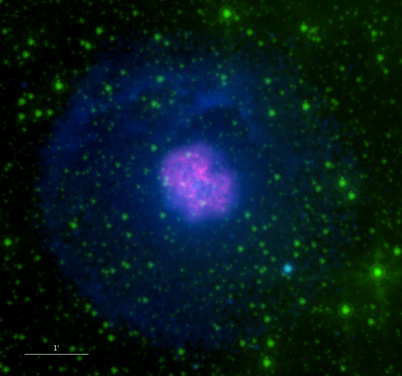
Figure 1: Multi-wavelength image of G21.5$-$0.9. From Chandra: 0.5–10 keV (Blue), VLA: 4.75 GHz (Pink) from Bietenholz & Bartel (2008), Spitzer: 5.8 microns (Green) Zajczyk et al. (2012). Note the 4.75 GHz data covers only the central PWN.

2 Observations

As a calibration target for the Chandra X-ray observatory, G21.5–0.9 was observed regularly by both the Advanced CCD Imaging Spectrometer (ACIS) and the High Resolution Camera (HRC). Recently, Matheson & Safi-Harb (2010) analyzed 578.6 ks (1999-2006) of ACIS observations to study limb-brightening in the eastern limb and search for thermal emission. In this work, we extend this study utilizing 86 ACIS observations totaling of 786.1ks (1999-2014) and 17 HRC observations with totalling of 306.1ks. Data processing was performed using the Chandra Interactive Analysis of Observations (CIAO) software package (Fruscione et al. (2006)), while spectral analysis made use of the X-ray Spectral fitting package XSPEC version 12.9.1 (Arnaud (1996)).

2.1 Structure

A multi-wavelength image is shown in Figure 1. The remnant G21.5$-$0.9 is dominated by a bright PWN (visible from radio (pink) through x-ray (blue)), which is 40^′′ in radius, centered at $\alpha(2000)=18^{h}33^{m}33.37^{s}$, $\delta(2000)=-10^{o}34^{\prime}06".25$ and powered by the central pulsar PSR J1833–1034. The diffuse emission is only revealed by deep x-ray observations, extends to a radius of 150^′′ and displays a limb-brightened eastern edge. Knots with enhanced soft x-ray emission appear to the north and merge with the limb-brightened edge to the east. The diffuse emission fills a circle coincident with the geometry of the limb-brightened eastern edge, but the additional $\sim 200$ks of ACIS data still do not reveal limb-brightening to the west. The diffuse emission merely blends with the background level. Point source SS 397 is located to the south west within the extended shell. Zajczyk et al. (2012) found infrared emission (green) from the inner 4^′′ but no extended emission at larger scales with the dominant contribution from field stars.

2.2 Brightness Profile

The presence of a dust scattering halo complicates analysis of the faint outer regions identified as the supernova shell. We use the wealth of observations to update the surface brightness profiles of Bocchino et al. (2005) and Matheson & Safi-Harb (2005). Profiles were extracted from quadrants of the merged event file and filtered into 4 energy bands: 0.3–1.5, 1.5–3, 3–5, and 5–8 keV. The results are shown in Figure 2. The bottom left quadrant shows the limb brightened edge revealed by Matheson & Safi-Harb (2005), the brightest knot is clearly visible in the top right profile. The top left shows the contribution from the fainter knot structures and the bottom right which displays no limb brightening smoothly declines to the background level.

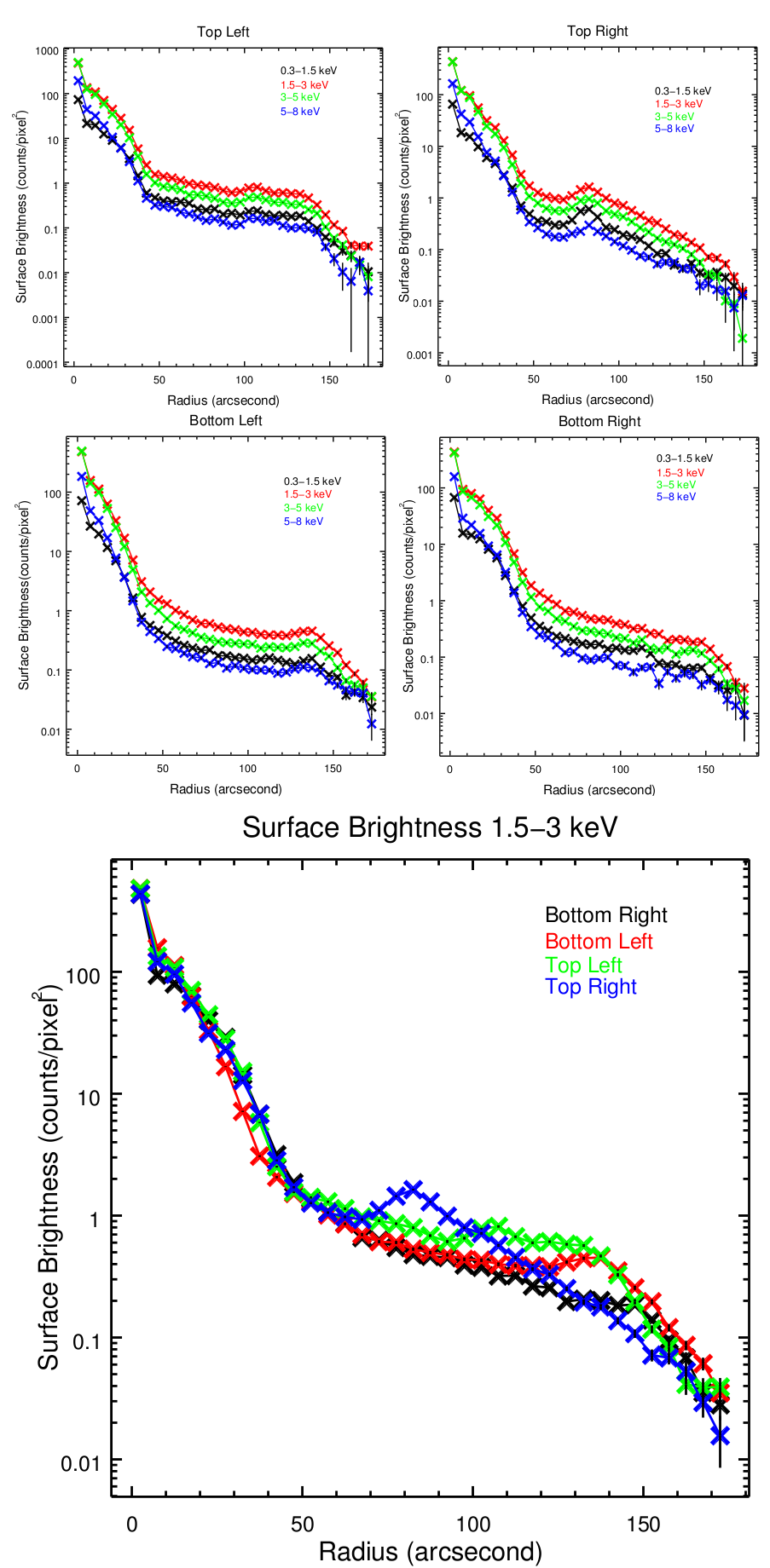
Figure 2: Upper panel: Surface brightness profiles of four quadrants of G21.5-0.9 at four different energy bands. Bottom panel: Overlay of the profile of each quadrant in the 1.5–3 keV band.

3 Spectroscopy

3.1 Processing

Weighted spectra were extracted for each observation using the CIAO routine specextract. Each spectrum has an associated background which is extracted from the same CCD chip, but outside the shell and is not overlapping with any regions listed in the Chandra Source Catalogue. The observations were processed with the CIAO 4.7 Chandra-repro script and is fitted simultaneously without merging the individual spectra as recommended by the Chandra X-ray Center. The fitting was performed with the X-ray Spectral analysis software XSPEC v12.9.1 over the range 0.5–8 keV.

3.2 Detector Contamination

Since the observational data are taken many years apart, we checked if the changing response affected our results. The build up of contaminants has a stronger effect on low energy emission (Marshall et al., 2004), which is likely to affect the derived column density. To explore a systematic change in this parameter, we extract spectra from the PWN, group them by year of observation and fit individually to an absorbed power-law. We adopt the Tuebingen-Boulder ISM absorption model (TBABS in XSPEC), which calculates the cross-section for X-ray absorption. The required ISM abundances were set to those from Wilms et al. (2000). The results of this analysis are presented in Fig.3. No general trend with increasing column density is found. Therefore, in what follows, we use the single best-fit value estimated with the total simultaneous fit in section 3.3.

Figure 3: Fitting observations of the PWN grouped by year to an absorbed power-law. The column density has units of $10^{22}$ atoms cm^-2. The dotted line marks the best fit value for all observations fit simultaneously. See §3.3 for details.

3.3 Pulsar Wind Nebula

In order to properly account for the absorption along the line of sight, spectra from the PWN were extracted from a 40^′′ circle centered at $\alpha(2000)=18^{h}33^{m}33.37^{s}$, $\delta(2000)=-10^{o}34^{\prime}06".25$. This was fit with an absorbed power-law with the absorption given by the TBABS model in XSPEC (see Table 1). The best fit parameter for the column density was frozen in subsequent region analysis to 3.237 $\times 10^{22}$ cm^-2 (see section 3.5 for further discussion).

Table 1: Spectral-fitting results for the pulsar wind nebula^a

$N_{H}(10^{22}$ atoms cm${}^{-2})$	3.237 (3.225 - 3.250)
$\Gamma$	1.841 (1.835 - 1.847)
Norm ($10^{-2}$)b	1.886 (1.869 - 1.903)
${\chi}^{2}_{\nu}(\nu)$	1.114 (26369)
Absorbed Flux ($10^{-11}$ erg cm-2 s-1)	4.555 $\pm$ 0.005
Luminosity($10^{35}$ erg s-1)c	2.822 $\pm$ 0.003
Effective Exposure	590.3 ks
a All confidence ranges are 90%. Models were fit over
the range 0.5-8 keV.
b Units are photons keV-1 cm-2 s-1
c Unabsorbed, assuming a distance of 5 kpc to G21.5$-$0.9

3.4 Spectral Map

To generate a photon index map, we applied the contour binning software contbin (Sanders, 2006), which produces adaptive bin size following the surface brightness of an input image, such that each bin meets a given signal limit. The exposure corrected merged flux counts image spanning the range 0.5–10 keV was used as input with a signal limit of 150. This corresponds to a limit of a few hundred counts in the resulting spectra for a single observation of each generated region. The spectra were fitted with an absorbed power-law and the absorption coefficient is frozen to the best fit value derived for the PWN (see section 3.3). The generated regions were coloured with their best fit value of the photon index, which is illustrated in Fig. 4. A zoomed in view of the small scale in the PWN is presented in Figure 5 with details. The non-symmetric nature of the emission is clearly shown in the figure, where the hardest emission is offset from the location of the PSR (marked with a cross) with a bubble of higher energy emission extending to the north.

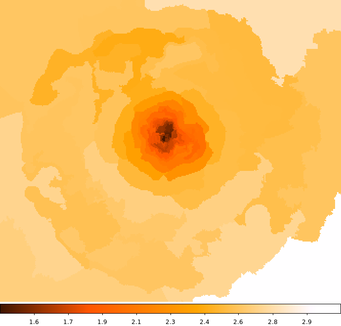
Figure 4: Photon index map for the entire remnant. The colourbar shows the power-law photon index, with the darker (lighter) colour reflecting a harder (softer) spectrum.

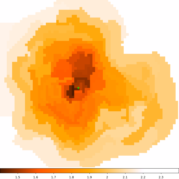
Figure 5: Photon index map zoomed in on the PWN. The green cross marks the position of the PSR. See §3.3.1 for details

3.5 Radial Profile

Spectra were extracted from rings centered on the pulsar, and fit with an absorbed power-law. The column density is found to be $3.237\times 10^{22}\,cm^{-2}$ for the external background region selection and $3.222\times 10^{22}\,cm^{-2}$ for the internal background selection. As shown in Fig. 6, the photon index is shown to increase to the edge of the PWN at 40^′′, which is consistent with previous studies (e.g. Matheson & Safi-Harb 2005). However, a higher column density is derived comparing with previous work (Slane et al. 2000, Safi-Harb et al. 2001, Warwick et al. 2001, Bocchino et al. 2005, Matheson & Safi-Harb 2010) , which is likely because we apply the TBABS model with $wilm$ abundances. We verify this by fitting the PWN spectra with the previously used WABS model for photoelectric absorption which uses the Wisconsin cross-sections (Morrison & McCammon (1983)) and find a smaller value of $2.37\pm 0.01\times 10^{22}$cm^-2 which is consistent with previously published results. To account for the halo emission, an annulus centred on the pulsar with radius 44^′′–48^′′ was chosen as background which had a negligible effect on the spectral index. This is expected due to the drop in surface brightness outside the PWN. Figure 2 shows that the surface brightness where the internal background was taken is fainter by a factor of more than 20 from the inner PWN. Therefore the dust scattered halo component leads to a systematic underestimation of the photon index errors, yet the overall result will remain unchanged. Additionally, the halo contributes minimally above 5 keV (Bocchino et al. (2005)) and when we restrict our fits to the range 5–8 keV we find the trend is unchanged. The high energy profile differs in that the pulsar component is not visible in the first data-point.

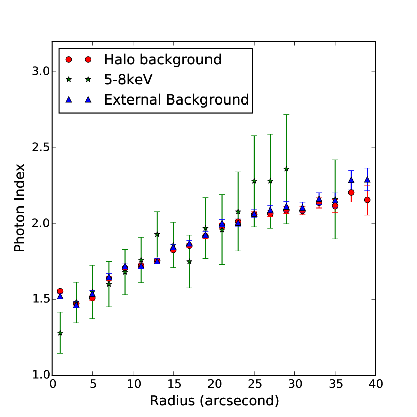
Figure 6: Photon index found for rings of increasing size within the central bright PWN. The External (triangles, blue symbols) and Halo (circles, red symbols) background profiles correspond to the 0.5–8 keV bands and use a background region outside and from within the halo, respectively. The 5–8 keV profile (stars, green points) also use the internal background, which is an annulus centred on the pulsar with a radius of 44^′′–48^′′ to minimize contribution from the dust scattering halo. Errorbars on the photon index are at the 90% confidence level.

The near linear increase of the spectral index with radius is consistent with that observed in other young PWNe, such as 3C 58 (Slane et al. (2004)). The spectral index continues to rise beyond the edge of the PWN at 40^′′, which reaches a maximum at 50^′′ and remains roughly flat to the edge of the remnant, see Figure 7. The model fitting of the spectral index profile will be discussed in detail in section 5.2. We include the best fit power-law parameters in the appendix to assist with future modeling work (see Tables A1-A4), and in spatially resolved spectroscopic studies of the whole remnant, including the halo and shell emission.

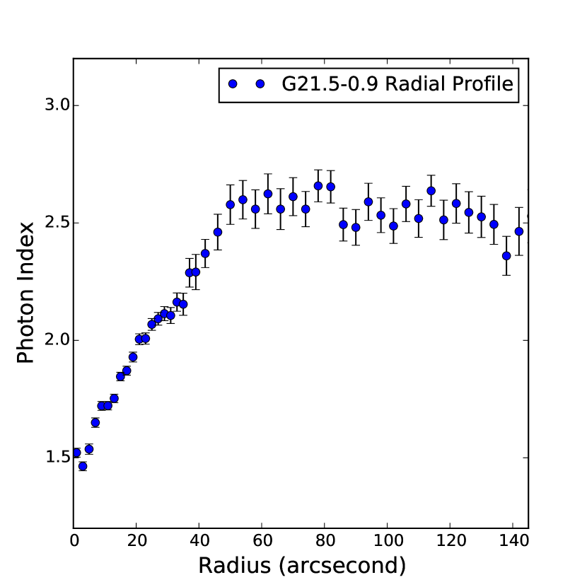
Figure 7: Spectral index vs radius fit for the entire remnant over 0.5–8 keV, with the absorption frozen to the best fit value found from fitting the PWN. The northern knot region coincides with the slight increase at 80^′′ and the limb-brightened edge of the remnant corresponds to the drop at 140^′′.

3.6 PSR J1833–1034

Evidence of weak thermal x-ray emission from the pulsar powering $G21.5-0.9$ has been suggested (Matheson & Safi-Harb 2010). To follow up on this study with the deeper exposure, we select a 2^′′ radius centred on the pulsar at $\alpha(2000)=18^{h}33^{m}33.54^{s}$, $\delta(2000)=-10^{o}34^{\prime}07.6"$ using observations with an off-axis angle less than 3^′. The background was extracted from a circular annulus centred on the PSR with radius 2^′′– 4^′′ to remove contamination from the PWN. The spectra were fitted with an absorbed power-law utilizing the best fit column density in the PWN. The fitting results are provided in Table 2, and a combined spectrum is shown in Figure 8. The single power-law model derives a hard spectral index $\Gamma=1.54\pm 0.02$ with $\chi^{2}_{\nu}(\nu)=1.075(3731)$. The addition of a thermal blackbody component improves the fit slightly, which yields a harder spectral index $\Gamma=1.35\pm 0.12$ with temperature $kT=0.43^{+0.04}_{-0.09}$ keV and $\chi^{2}_{\nu}(\nu)=1.072(3729)$. F-test is a statistical measure of the requirement of an additional model based on improvement in the reduced chi-squared value vs the change in the number of degrees of freedom. We find that the thermal component is required over a power-law alone with an F-test probability of 7.6$\times 10^{-3}$. This is notably less significant than the previous result by Matheson & Safi-Harb (2010), which found a probability of $2.6\times 10^{-4}$.

Figure 8: Combined spectra of the PSR with the simultaneous model fit (solid line), power-law and blackbody components (dashed lines).

Table 2: Spectral-fitting results for PSR J1833–1034.

Model	Model Parameter	PSR
	Effective Exposure	280.2 ks
Power-law	$N_{H}(10^{22}$ atoms cm${}^{-2})$	3.237 (Frozen)
	$\Gamma$	1.54 (1.52 - 1.56)
	Norm ($(10^{-4})^{a})$	8.34 (8.13 - 8.57)
	${\chi}^{2}_{\nu}(\nu)$	1.075 (3731)
	Flux ($10^{-12}$)b	3.19 $\pm$ 0.02
Power-law	$N_{H}(10^{22}$ atoms cm${}^{-2})$	3.237 (Frozen)
+	$\Gamma$	1.35 (1.23 - 1.46)
Blackbody	Norm ($(10^{-4})^{a})$	6.14 (5.04 - 7.08)
	kT (keV)	0.43 (0.34 - 0.47)
	Norm ($(10^{-6})^{c})$	5.74 (2.89 - 8.68)
	${\chi}^{2}_{\nu}(\nu)$	1.072 (1421)
	Flux ($10^{-12}$)b	3.16 (3.13 - 3.18)
	Thermal flux($10^{-13}$)b	1.18
	Non-thermal flux ($10^{-12}$)b	3.04
	Thermal flux ($10^{-13}$)d	4.57
a photons keV-1 cm-2 s-1
b Observed flux in units of erg cm-2 s-1
c $L_{39}/D^{2}_{10}$
d Unabsorbed flux in units of erg cm-2 s-1

3.7 Northern Knot

The bright knot to the north of the PWN appears as a region of enhanced soft X-ray emission. Previous studies suggested a two-component model with both thermal and non-thermal emission. However, the thermal emission component was not well constrained. Bocchino et al. (2005) found evidence for thermal emission in the ‘North Spur’, which is characterized by a two-component power-law plus vnei model. The fitting to Chandra and XMM-Newton data produced two minima: one is consistent with solar abundances and the other with enhanced abundance of Si (2–20 times solar) and Mg (0.6–3 times solar). Matheson & Safi-Harb (2010) show the northern knot is dominated by non-thermal emission while the thermal component comprising only 6% of the observed flux. The abundances are more consistent with the solar abundances provided by Bocchino et al. with $Mg$ = 0.72 (0.40–1.06), $Si$ = 0.84 (0.32–1.35) although also included a large (albeit poorly constrained) abundance of Sulphur, $S$ = 107 (4–210). In addition to the two-component model, we fit the data with thermal and non-thermal models separately. The results (see Table 3 and Figure 9) are consistent with the previous Chandra study. The thermal model requires solar abundances but a higher temperature. The addition of a non-thermal component improves the fit, meanwhile lowering the required temperature and enhancing the abundance of Si. The abundance of Si is poorly constrained and tied to the VPSHOCK normalization. When both parameters are allowed to vary, there is no plausible upper limit found on the Si abundance; however the lower limit is still characteristic of enhancement. In order to place plausible constraints on the abundance, the normalization of the VPSHOCK model was frozen at its best fit value for the calculation of the Silicon error range. Our results are consistent with the 2nd minima discussed in Bocchino et al. (2005) and supports the interpretation of an ejecta knot of Si. Assuming the emitting volume is an ellipsoid with $V=1.77\times 10^{55}D_{5}fcm^{3}$, where $f$ is the filling factor, we estimate the density of the emitting plasma to be $42$ cm^-3, which is significantly higher than the ambient density calculated in section 3.8.

Figure 9: Combined Spectra of the knot plotted with the simultaneous fit result for a power-law + VPSHOCK model. See text for details.

Table 3: Spectral-fitting results for the northern knot. See text for details.

Model	Parameter	Northern Knot
	Effective Exposure	509.4 ks
	$N_{H}(10^{22}$ atoms cm${}^{-2})$	3.237 (Frozen)
Power-law	$\Gamma$	2.62 (2.578-2.67)
	Norm ($10^{-4}$)a	3.67 (3.51-3.84)
	${\chi}^{2}_{\nu}(\nu)$	1.306 (815)
	Flux ($10^{-13}$)b	3.12 (3.07-3.16)
vpshock	kT (keV)	4.2 (3.8-4.7)
	Mg	0.56 (0.39-0.72)
	Si	0.31 (0.24-0.39)
	S	0.16 (0.04-0.28)
	$n_{et}(10^{10}$cm-3 s)	2.86 (1.70-4.75)
	Norm ($10^{-4}$ cm-5)	5.04 (4.64-5.55)
	${\chi}^{2}_{\nu}(\nu)$	1.062 (811)
	Flux ($10^{-13}$)b	3.33 (3.27-3.36)
Power-law	$\Gamma$	2.24 (2.17-2.31)
+	Norm ($10^{-4}$)a	2.51 (2.28-2.72)
vpshock	kT (keV)	0.15 (0.12-0.17)
	Mg	0.77 (0.35-1.72)
	Si	15.7 (7.7-26.2)
	$n_{et}$($10^{13}$ cm3 s-1)	5.0 ($>$0.3)
	Norm (cm-5)	0.102 (0.042-0.177)
	${\chi}^{2}_{\nu}(\nu)$	1.041 (1178)
	Flux ($10^{-13}$)b	3.20 (3.04-3.21)
	Non-thermal flux ($10^{-13}$)b	3.05
	Thermal flux ($10^{-13}$)b	0.15
Power-lawc	$\Gamma$	2.55 (Frozen)
+	Norm ($10^{-4}$)a	2.70 (1.64-2.96)
Power-law	$\Gamma$	1.3 (0.4-2.1)
+	Norm ($10^{-5}$)a	2.0 (1.6-8.0)
vpshock	kT (keV)	0.14 (0.13-0.15)
	Mg	1.1 (0.5-1.8)
	Si	37 (5-118)
	$n_{et}$($10^{13}$ cm3 s-1)	2.7 ($>$0.04)
	Norm (cm-5)	0.14 (0.08-0.28)
	${\chi}^{2}_{\nu}(\nu)$	1.041 (1176)
a Photons keV-1 cm-2 s-1
b Observed flux in erg cm-2 s-1
c Dust scattering halo component

The dust scattering halo complicates the analysis of the faint thermal emission. To better understand its effect on our fits we extract a background from an annulus surrounding the knot. The general result does not change. We find a power-law photon index and temperature that are consistent (within error) with the external background. The abundances show the same trend with an approximately solar abundance of Mg and an enhanced abundance of Si; however the parameters are less bound with the upper limit for Si remaining unconstrained. Alternatively, we try adding an additional power-law component with its photon index fixed to the value at which the radial profile (see Figure 7) appears to level off, and allow the normalization to vary. Again, the thermal parameters are consistent with the previous result. A harder photon index of 1.3 is found for the non-thermal component yet this addition does not improve the fitting statistic (see Table 3).

3.8 Eastern Limb

The nature of the extended emission surrounding the central PWN in G21.5$-$0.9 has been a puzzle since the first Chandra observations (Slane et al. (2000); Safi-Harb et al. (2001)). Models including dust scattering and shock heated ejecta have been proposed. Imaging analysis by Matheson & Safi-Harb (2010) found limb-brightening along the south eastern edge of the remnant, concluding that the dust scattering halo could not account for the total extended emission. Spectral analysis found an unreasonably high temperature for the emission to be purely thermal, which implied particle acceleration rather than shock-heated ejecta (Matheson & Safi-Harb 2010). Nynka et al. (2014) found an excess of emission above 10 keV in the direction of the eastern limb with NuSTAR data, which further support the non-thermal model. Our results are presented in Table 4, with a combined spectra shown in Figure 10. The spectrum is best explained with a two-component power-law plus PSHOCK model. The emission is primarily non-thermal and the thermal component contributes only 3.5% of the total flux. Although the thermal contribution is small, it is statistically required with a F-test probability of $2.7\times 10^{-11}$. No emission lines are observed and the thermal component is characterized by a temperature $kT=0.37$ keV and small ionization time-scale $n_{et}=6.57\times 10^{9}$ cm^-3 s (see Table 4). For a limb emitting volume of $6\times 10^{56}D^{3}_{5}fcm^{3}$, where $f$ is the filling factor, the small amount of thermal emission suggests an emitting density of 1.76 cm^-3. The explosion energy implications of this density are further discussed in section 5.3.

Figure 10: Combined Limb spectra plotted with the simultaneous fit to a power-law + PSHOCK model.

Table 4: Spectral-fitting results for the eastern limb. See text for details.

Model	Parameter	Eastern Limb
	Effective Exposure	318.7 ks
	$N_{H}(10^{22}$ atoms cm${}^{-2})$	3.237 (Frozen)
Power-law	$\Gamma$	2.49 (2.44-2.54)
	Norm ($10^{-4}$)a	5.36 (5.11-5.63)
	Flux ($10^{-13}$)b	5.38 (5.32-5.45)
	${\chi}^{2}_{\nu}(\nu)$	1.016 (1040)
pshock	kT (keV)	3.04 (2.85-3.37)
	$n_{et}$($10^{12}$ cm3 s-1)	2.07 (0.97-4.78)
	Norm ($10^{-4}$ cm-5)	9.73 (8.87-10.02)
	${\chi}^{2}_{\nu}(\nu)$	1.177 (1039)
	Flux ($10^{-13}$)b	5.49 (5.42-5.58)
Power-law	$\Gamma$	2.22 (2.04-2.34)
+	Norm ($10^{-4}$)a	3.76 (2.90-4.41)
pshock	kT (keV)	0.37 (0.20-0.64)
	$n_{et}$($10^{9}$ cm3 s-1)	6.57 ($<29.5$)
	Norm ($10^{-3}$ cm-5)	6.21 (1.25-96.18)
	${\chi}^{2}_{\nu}(\nu)$	0.966 (1037)
	Flux ($10^{-13}$)b	5.61 (5.37-5.67)
	Non-thermal flux ($10^{-13}$)b	5.41
	Thermal flux ($10^{-13}$)b	0.20
Power-lawc	$\Gamma$	2.55 (Frozen)
+	Norm ($10^{-4}$)a	4.3 (0-4.9)
Power-law	$\Gamma$	1.5 (0.5-2.3)
+	Norm ($10^{-5}$)a	3.7 (0.6-44.6)
pshock	kT (keV)	0.23 (0.15-0.37)
	$n_{et}$($10^{13}$ cm3 s-1)	5 (Unconstrained)
	Norm ($10^{-3}$ cm-5)	4.2 (1.1-36.8)
	${\chi}^{2}_{\nu}(\nu)$	0.966 (1036)
a Photons keV-1 cm-2 s-1
b Observed flux in erg cm-2 s-1
c Dust scattering halo component

In order to decouple the scattered halo emission from the limb itself, we extract a background from just inside the limb, with a similar treatment to the northern knot. However the limb brightening is not significant enough to provide robust statistics. Instead we add a power-law component with the photon index fixed to the leveled off value from the radial profile and allow the normalization to vary. With this added non-thermal component we again find a faint thermal contribution with temperature of 0.23 keV (Table 4) - consistent within error of our non-halo result and a photon index of 1.5. Again, the added component does not improve the fitting statistic.

4 Variability in the Pulsar Wind Nebula

Bright Knots, which appear and fade away on time-scales of weeks to months with velocities of $\sim 0.5c$, have been observed in PWNe such as the Crab and Vela nebulae (Hester et al., 2002; Pavlov et al., 2001). We searched for such features in G21.5$-$0.9 with the HRC observations from the same date, which were merged and normalized to 20 ks exposures. Figure 11 shows the result. The same process was followed for the ACIS observations, which are displayed in Figure 12. The images are available as a video slide show in the online journal. Unlike the Crab and Vela nebulae, G21.5$-$0.9 does not show persistent structure in the PWN. To reveal changes, difference images (see Figure 13) were created by subtracting one set of observations from the next.

If we assume that the features we see are persistent structures which have moved rather than new wisps which formed between observations we can calculate the velocity required. Tracking several bright knots we find velocities of 0.2–0.75 c with an average of 0.5 c. Performing the same analysis on the ACIS observations yields consistent results.

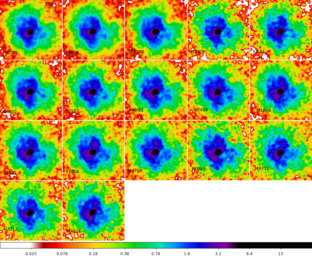
Figure 11: Variability seen with HRC.

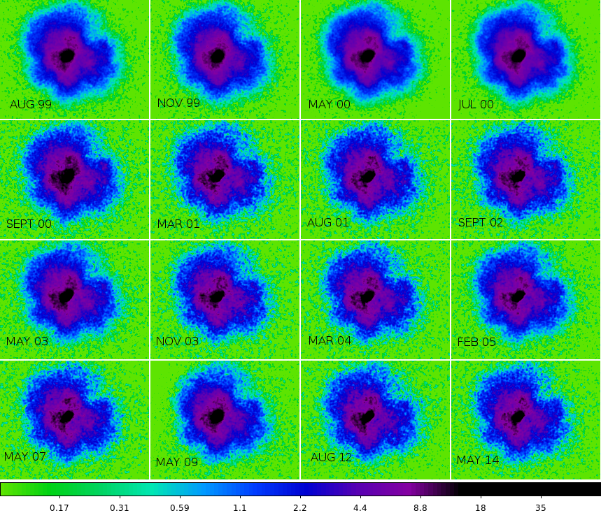
Figure 12: Variability seen with ACIS

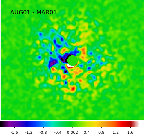
Figure 13: Sample ACIS difference image. The PSR has been removed to highlight the faint changes

5 Discussion

5.1 Pulsar J1833-1034

The spectra of PSR J1833–1034 can be fitted reasonably well with a single power-law. The addition of a thermal blackbody component does improve the fit but only marginally. The F-test probability of 0.17 indicates that this component is unimportant compared to the previous result of Matheson & Safi-Harb (2010).We assume this thermal component is real and then examine the effect of the fit on the pulsar parameters. We assume black-body radiation, i.e., $L=4\pi R^{2}\sigma T^{4}$. The unabsorbed thermal flux of $4.57\times 10^{-13}$ erg cm^-2 s^-1 at a distance of 5 kpc and temperature of 0.43 keV suggest an emitting region of 0.6 km in size, which is much smaller than the canonical radius of a neutron star and is consistent with the previous suggestion that the source is a small hot spot on the neutron star surface. The spectral map of the PWN (Figure 5) reveals that the PSR is offset from the regions of harder spectra. If we attribute this offset to the termination shock radius, then the nebular magnetic field can be estimated as follows. Given the spin-down energy loss $\dot{E}=3.37\times 10^{37}$ erg s^-1 (Camilo et al., 2006), $\theta_{s}=0.46^{\prime\prime}\eta^{-1/2}d^{-1}_{5}B^{-1}_{mG}$, where $\theta_{s}=r_{s}/d$, $\eta$ is the filling factor of pulsar wind and $B_{mG}$ is the nebular magnetic field in mG. The offset of 3^′′.5 suggests a magnetic field of 0.13 mG.

5.2 Pulsar wind nebula

Kennel & Coroniti (1984a, b) (hereafter KC) treat the pulsar wind as magnetohydrodynamic (MHD) flow and then derive the steady-state particle and magnetic field structure in the PWN with spherical symmetry and a purely advective wind flow. The KC model was able to explain the spectral and spatial distribution of the optical and X-ray emission in the Crab Nebula, but failed in the radio band. The discovery of axisymmetric jet-torus structures in PWNe like the Crab nebula with high resolution X-ray and optical imaging (e.g. Weisskopf et al., 2000; Hester, 2008) motivates 2-dimensional (2D) MHD simulations of PWNe with anisotropic pulsar wind power. Current 2D MHD simulations are able to reproduce the jet-torus structure and the inner ring feature in PWNe with polar angle dependent pulsar wind power (e.g. Komissarov & Lyubarsky, 2003; Del Zanna et al., 2006). However, toroidal structures are only detected in the inner part of the nebula (e.g. Safi-Harb et al., 2001; Slane et al., 2004; Hester, 2008), where the impact of the pulsar wind is crucial. In the outer part of the nebula, complex filamentary structures with fingers and loops are instead observed (e.g. Seward et al., 2006; Hester, 2008). It is found that the standard MHD model ran into problems to explain the spectral index distribution and surface brightness profile in the outer part of the nebula (Amato et al., 2000; Slane et al., 2004). The polarization measurements (e.g. Hester, 2008) and the deep Chandra images (e.g. Seward et al., 2006) indicate that the magnetic topology in the filamentary structure is much more complicated than the toroidal field assumed in the standard MHD model.

Tang & Chevalier (2012) show that the introduction of diffusive particle transport in PWNe can explain the spectral index distribution and the nebular size behavior in young PWNe like the Crab and 3C 58 very well. It is assumed that advection plays a dominant role in the inner part of the nebula with toroidal structure, while diffusion becomes dominant in the outer part of the nebula with filamentary structure. The exact nature of diffusion is still unclear, and is likely induced by the Rayleigh-Taylor (RT) instability at the outer boundary of the nebula (e.g. Chevalier & Gull, 1975; Jun, 1998) or/and the kink instability triggered at the TS (e.g. Begelman, 1998; Camus et al., 2009). These fluid instabilities may be able to destroy the ordered toroidal field, which is imposed by the pulsar wind, and drive turbulence in the PWN. Recent 3-dimensional MHD and test particle simulations reveal a turbulent nebula with high velocity fluctuation (Porth et al., 2016), which indicates efficient diffusive transport of particles in PWNe. The effective diffusion coefficient is estimated as (Porth et al., 2016).

$$D_{eff}\sim 2\times 10^{27}~{}\left(\frac{L_{TS}}{0.13\rm pc}\right)~{}\rm cm^{2}s^{-1}$$ (1)

which is found to be independent of energy for electrons up to PeV energy. $L_{TS}$ is the radius of TS.

In Fig. 14, we fit the spectral index distribution between $0.5$ keV and $8$ keV in G21.5-0.9 with both the KC model and a pure diffusion model (Tang & Chevalier, 2012) assuming simple spherical symmetry. The red dashed line represents the KC model results with $\sigma=3\times 10^{-3}$, $\alpha=1.9$ and $B_{TS}=50\mu G,$ where $\sigma$ is the Poynting flux to particle energy flux ratio at the TS, $\alpha$ is the power law index of the injected particle spectrum and $B_{TS}$ is the magnetic field at the TS. $\sigma$ is chosen to be $3\times 10^{-3}$ to match the expansion velocity of $910$ km/s at the outer boundary of G21.5–0.9 (Bietenholz & Bartel, 2008). It is clear that the KC model is inconsistent with the spectral index distribution in G21.5–0.9, which is similar to the previous study of 3C 58 (Slane et al., 2004). The blue solid line presents the diffusion model results with $\alpha=1.9$, $D\sim 2.1\times 10^{27}\rm cm^{2}/s$ and $B=130\mu G$ (see §5.1). $D$ and $B$ are the diffusion coefficient and magnetic field respectively, which are assumed to be constant for simplification and should be understood as the spatial averaged values in the PWN. The angular radius of the TS is assumed to be $\theta_{s}\sim$3^′′.5. It is interesting to note that the effective diffusion coefficient $D_{eff}$ defined in eq. (1) is estimated to be $\sim 1.3\times 10^{27}\rm cm^{2}/s$ with $L_{TS}\sim 0.08$pc, which agrees with our diffusion model results.

In the pure diffusion model, the photon index distribution of the nebula is determined by the dimensionless ratio $\zeta=r^{2}/Dt_{c}$, where $r$ is the radius and $t_{c}$ is the cooling time scale. If $\zeta\ll 1$, the photon index distribution is very flat. If $\zeta\gtrsim 1$, the photon index distribution gradually steepens as $\zeta$ increases. For synchrotron-dominated cooling, $\zeta\propto r^{2}B^{3/2}\nu^{1/2}/D$, where $\nu$ is the corresponding emission frequency. The diffusion coefficient of charged particles in a nebula depends on the magnetic field configuration and the Larmor radius. The nature of this magnetic field dependence is not fully understood yet. In the limit of Bohm diffusion, $D\propto B^{-1}$ and $\zeta\propto r^{2}B^{5/2}\nu^{1/2}$ which is considered to be a reasonable choice in the presence of strong turbulence (e.g., Hussein & Shalchi, 2014). Field line random walk represents another limiting case, in which magnetic field lines wander due to turbulence and the particles follow the field lines exclusively. In this case, the diffusion coefficient scales as $D\propto B^{-2}$ and $\zeta\propto r^{2}B^{7/2}\nu^{1/2}$ (e.g., Shalchi, 2009). The magnetic dependence of $D$ in the nebula is likely between the two limiting cases.

The spatial dependence of the magnetic field in the nebula is very complicated according to 2D and 3D MHD simulations (Del Zanna et al., 2006; Porth et al., 2016), which is beyond the scope of this work. Here we briefly discuss the magnetic configuration in the KC model. Behind the termination shock, the magnetic field evolves as $B\propto r$ due to the flux freezing. As $r$ increases, the magnetic pressure gradually becomes dominant. After that, the radial speed is approximately constant and $B\propto r^{-1}$ instead. In the $B\propto r$ regime, which corresponds to the inner part of the nebula, we have $\zeta\propto r^{9/2}$ for Bohm diffusion and $\zeta\propto r^{11/2}$ for field line random walk respectively. If $\zeta$ increases with radius, we expect the photon index distribution steepens much faster with radius compared to our simplified calculation with constant $D$ and $B$. In the $B\propto r^{-1}$ regime, which corresponds to the outer part of the nebula, we instead have $\zeta\propto r^{-1/2}$ and $\zeta\propto r^{-3/2}$ for the two limiting cases of diffusion. If $\zeta$ decreases with radius, the photon index distribution becomes more flat compared to our simplified calculation. In summary, if we consider the spatial dependence of $B$ and $D$ described above, then the photon index distribution steepens in the inner region and flattens in the outer region, which appears to be more consistent with the data of G21.5–0.9.

Based on the above discussion, when $D\propto B^{3/2}$, $\zeta$ is the same and the photon index distribution remains almost the same. If we instead assume $B=50\mu G$ as indicated by de Jager et al. (2008), then we obtain $D\sim 5\times 10^{26}\rm cm^{2}/s$, which is consistent with the results derived in Porth et al. (2016) based on 3D MHD simulations. Recently, G21.5–0.9 was discussed by Lu et al. (2017) with an improved model including dynamical evolution of the central pulsar, energy dependence of diffusion coefficient $D$, and radial dependence of diffusion coefficient $D$ and magnetic field $B$. It is not straightforward to compare with their fitting results directly. Here we only consider the spatially averaged value derived at present day. Lu et al. (2017) found that $B\sim 40\mu G$ and $D\sim 1\times 10^{26}cm^{2}s^{-1}$ for the energy range of interest here, which is consistent with our simple toy model results surprisingly well (we note that the diffusion coefficient shown in Table 2 of Lu et al. (2017) is at a much lower electron energy). According to the above discussion, if we assume the diffusion coefficient provided in eq (1) is a good approximation, then we can decouple $D$ and $B$ in the pure diffusion model and apply the model to estimate the spatially averaged magnetic field in a PWN.

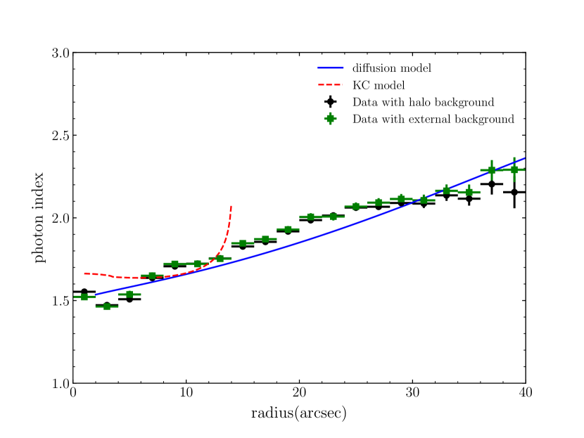
Figure 14: Fitting of the photon index distribution between $0.5$ keV and $8$ keV in G21.5–0.9. The black and green crossings are the data with halo and external background respectively. The blue solid line is the pure diffusion model fitting with $\alpha=1.9$, $B=130\mu G$ and $D\sim 2.1\times 10^{27}\rm cm^{2}/s$. The red dashed line is the KC model fitting with $\alpha=1.9$, $B_{TS}=50\mu G$ and $\sigma=3\times 10^{-3}$.

5.3 Supernova Remnant

The absence of a shell-like structure surrounding some PWNe is a long standing puzzle. Whether the undetected shells are due to expansion into a very low density medium or a consequence of a low energy electron-capture supernova explosion (e.g., Nomoto et al. (1982); Yang & Chevalier (2015)) remains an open question. Deep observations revealed thermal emission in 3C 58 (Bocchino et al., 2001; Gotthelf et al., 2007) and G54.1+0.3 (Bocchino et al., 2010), which is attributed to the missing shells and/or shock-heated supernova ejecta. The faint thermal emission detected in the eastern limb may be used to calculate the shock speed and estimate the energy released during the supernova event. The Rankine-Hugoniot relations for an adiabatic shock (Reynolds, 2008) yield $kT=\frac{3}{16}\mu m_{p}v^{2}_{s}$, where $\mu$ is the mean mass per particle ($\mu\approx 0.6$), $m_{p}$ is the proton mass and $v_{s}$ is the shock speed. The observed temperature of 0.37 keV corresponds to a shock speed of 562 km/s. Assuming a constant shock velocity and 5 kpc distance, the 140^′′ shell radius gives an age of 1.2 kyr, which is slightly larger than the 870 years derived from radio observations of the nebula expansion with a velocity of 910 km/s. For young remnants with an age less than 1000 years, the forward shock speed is expected to be higher. Although the derived temperature is low, it is consistent with that found in 3C 58 (Gotthelf et al., 2007; Bocchino et al., 2001), which is described by a dominant non-thermal component with $\Gamma\sim 2-3$ and a weaker thermal component with $kT\sim 0.2$ keV. However, 3C58 is older, and more evolved, with the thermal emission residing at the outer boundary of the PWN rather than a distinct and separate limb-brightened component. The low temperature may indicate a non-equilibrium state of the electrons and ions as suggested by Hughes et al. (2000), therefore we note that the estimated shock velocity scales as $\sqrt{T_{p}/T_{e}}$. We use the thermal component to calculate the ambient density into which the shock wave is expanding. For a limb emitting volume of $6\times 10^{56}D^{3}_{5}fcm^{3}$, where $f$ is the filling factor, we find a number density of $1.76~{}cm^{-3}$ which corresponds to a limb mass of $\sim 1M_{\odot}$. If we assume this is the swept-up mass, then the remnant must be expanding into a low-density medium with $n_{e}\sim 0.19~{}cm^{-3}$, which is smaller than the upper limit of $0.65~{}cm^{-3}$ provided by Bocchino et al. (2005). Extending the limb to a full sphere, we estimate the kinetic energy of the supernova to be $3\times 10^{49}$ erg, which is much smaller than the $10^{51}$ erg expected for a typical supernova. The minimal thermal emission may indicate the SNR is expanding into the wind blown bubble produced by its progenitor. Elwood et al. (2017) predicts cavities with radii of $\approx$ 2–20 pc. G21.5$-$0.9 is consistent with the lower limit of this range. The low mass loss prior to a type IIP supernova combined with the wind blown cavity suggests the shock has not yet swept up enough mass to transition into a Sedov-Taylor phase.

Future observations with a sensitive, high-resolution, spectrometer such as the X-Ray Imaging and Spectroscopy Mission ($XRISM$, formerly known as $XARM$) in the near future, and $ATHENA$ in the more distant future, should reveal the missing thermal X-ray emission from the shocked ambient or circumstellar material in G21.5–0.9 and other shell-less PWNe.

Appendix A PWN Radial Profile data

Table 5: Spectral fit data found for the 5–8 keV radial profile with a background taken from inside the halo. The absorption model TBABS is frozen at 3.222$\times$10²² cm^-2. Errors quoted are 90% confidence levels.

Radius	$\Gamma$	error	Norm ($10^{-4}$)	error ($10^{-4}$)
(arcsec)		$\pm$		$\pm$
0-2	1.28	0.14	6	2
2-4	1.48	0.13	9	2
4-6	1.55	0.18	7	3
6-8	1.60	0.15	8	3
8-10	1.68	0.15	11	3
10-12	1.76	0.15	14	4
12-14	1.93	0.15	17	5
14-16	1.86	0.15	14	5
16-18	1.75	0.18	10	4
18-20	1.97	0.20	13	5
20-22	1.96	0.23	10	5
22-24	2.08	0.26	11	6
24-26	2.28	0.30	13	9
26-28	2.28	0.31	12	9
28-30	2.36	0.36	11	10
30-40	2.16	0.26	16	10

Table 6: Spectral fit data for the whole SNR in the 0.5–8 keV radial profile with a background taken from inside the halo. The absorption model TBABS is frozen at 3.222$\times$10²² cm^-2. Errors quoted are 90% confidence levels.

Radius	$\Gamma$	error	Norm ($10^{-4}$)	error ($10^{-4}$)
(arcsec)		$\pm$		$\pm$
0-2	1.55	0.01	10.1	0.2
2-4	1.47	0.01	9.2	0.1
4-6	1.51	0.01	6.8	0.1
6-8	1.64	0.02	8.4	0.1
8-10	1.71	0.01	11.3	0.2
10-12	1.72	0.01	13	0.2
12-14	1.76	0.01	13.2	0.2
14-16	1.83	0.01	13.3	0.2
16-18	1.85	0.01	12.5	0.2
18-20	1.92	0.02	11.5	0.2
20-22	1.99	0.02	10.6	0.2
22-24	2.01	0.02	9.7	0.2
24-26	2.06	0.02	9.1	0.2
26-28	2.07	0.02	8.3	0.2
28-30	2.09	0.02	6.9	0.2
30-32	2.09	0.03	5.2	0.2
32-34	2.14	0.03	4	0.1
34-36	2.12	0.04	2.7	0.1
36-38	2.20	0.06	1.8	0.1
38-40	2.16	0.1	1	0.1

Table 7: Spectral fit data found for the whole SNR in the 0.5–8 keV radial profile with a background taken from outside the observed SNR shell. The absorption model TBABS is frozen at 3.237$\times$10²² cm^-2. Errors quoted are 90% confidence levels.

Radius	$\Gamma$	error	Norm ($10^{-4}$)	error ($10^{-4}$)
(arcsec)		$\pm$		$\pm$
0-2	1.52	0.02	9.5	0.2
2-4	1.46	0.02	8.9	0.2
4-6	1.54	0.02	7.0	0.2
6-8	1.65	0.02	8.6	0.2
8-10	1.72	0.02	11.7	0.3
10-12	1.72	0.02	13.3	0.3
12-14	1.75	0.02	13.4	0.3
14-16	1.85	0.02	13.9	0.3
16-18	1.87	0.02	13.0	0.3
18-20	1.93	0.02	12.1	0.3
20-22	2.01	0.02	11.2	0.3
22-24	2.01	0.02	10.1	0.3
24-26	2.07	0.03	9.8	0.3
26-28	2.09	0.03	9.2	0.3
28-30	2.11	0.03	7.7	0.3
30-32	2.11	0.03	6.0	0.2
32-34	2.16	0.04	4.9	0.2
34-36	2.15	0.05	3.6	0.2
36-38	2.29	0.06	2.8	0.2
38-40	2.29	0.08	2.1	0.2
40-44	2.37	0.06	3.1	0.2
44-48	2.46	0.08	2.5	0.2
48-52	2.58	0.08	2.5	0.2
52-56	2.60	0.08	2.5	0.2
56-60	2.56	0.08	2.4	0.2
60-64	2.62	0.09	2.6	0.2
64-68	2.60	0.09	2.3	0.2
68-72	2.61	0.08	2.7	0.2
72-76	2.56	0.08	2.9	0.2
76-80	2.66	0.07	3.7	0.3
80-84	2.65	0.07	3.9	0.3
84-88	2.49	0.07	3.1	0.2
88-92	2.48	0.08	2.7	0.2
92-96	2.59	0.08	2.9	0.2
96-100	2.53	0.07	2.8	0.2
100-104	2.49	0.07	2.8	0.2
104-108	2.58	0.08	3.0	0.2
108-112	2.52	0.08	2.6	0.2
112-116	2.64	0.07	4.1	0.3
116-120	2.51	0.08	2.5	0.2
120-124	2.58	0.08	2.5	0.2
124-128	2.55	0.09	2.3	0.2
128-132	2.53	0.09	2.3	0.2
132-136	2.49	0.09	2.4	0.2
136-140	2.36	0.08	2.0	0.2
140-144	2.46	0.10	1.8	0.2
144-148	2.53	0.11	1.6	0.2
148-152	2.66	0.13	1.6	0.2
152-156	2.65	0.17	1.2	0.2
156-160	2.96	0.20	1.2	0.2

Table 8: Spectral fit data for the dust scattering halo. Spectra were extracted from annuli segments spanning 280-360 degrees where the SNR does not display limb brightening or knot features and beginning outside the edge of the PWN. The absorption model TBABS is frozen at $3.237\times 10^{22}cm^{-2}$. Errors quoted are 90% confidence levels.

Radius	$\Gamma$	error	Norm ($10^{-4}$)	error ($10^{-4}$)
(arcsec)		$\pm$		$\pm$
45-55	2.47	0.12	1.4	0.2
55-65	2.49	0.15	1.1	0.2
65-75	2.40	0.17	1.0	0.2
75-85	2.63	0.17	1.1	0.2
85-95	2.54	0.17	1.0	0.2
95-105	2.64	0.17	1.1	0.2
105-115	2.54	0.19	0.8	0.2
115-125	2.96	0.21	1.0	0.2
125-135	2.52	0.20	0.8	0.2
135-145	2.58	0.18	1.0	0.2
145-155	2.48	0.19	0.8	0.2
155-165	2.60	0.30	0.5	0.2

References

- Abdo et al. (2013) Abdo A. A., et al., 2013, ApJS, 208, 17
- Aharonian et al. (2018) Aharonian F., et al., 2018, PASJ,
- Amato et al. (2000) Amato E., Salvati M., Bandiera R., Pacini F., Woltjer L., 2000, A&A, 359, 1107
- Arnaud (1996) Arnaud K. A., 1996, in Jacoby G. H., Barnes J., eds, Astronomical Society of the Pacific Conference Series Vol. 101, Astronomical Data Analysis Software and Systems V. p. 17
- Bandiera & Bocchino (2004) Bandiera R., Bocchino F., 2004, Advances in Space Research, 33, 398
- Becker & Kundu (1976) Becker R. H., Kundu M. R., 1976, ApJ, 204, 427
- Becker & Szymkowiak (1981) Becker R. H., Szymkowiak A. E., 1981, ApJ, 248, L23
- Begelman (1998) Begelman M. C., 1998, ApJ, 493, 291
- Bietenholz & Bartel (2008) Bietenholz M. F., Bartel N., 2008, MNRAS, 386, 1411
- Bietenholz et al. (2011) Bietenholz M. F., Matheson H., Safi-Harb S., Brogan C., Bartel N., 2011, MNRAS, 412, 1221
- Bocchino et al. (2001) Bocchino F., Warwick R. S., Marty P., Lumb D., Becker W., Pigot C., 2001, A&A, 369, 1078
- Bocchino et al. (2005) Bocchino F., van der Swaluw E., Chevalier R., Bandiera R., 2005, A&A, 442, 539
- Bocchino et al. (2010) Bocchino F., Bandiera R., Gelfand J., 2010, A&A, 520, A71
- Camilo et al. (2006) Camilo F., Ransom S. M., Gaensler B. M., Slane P. O., Lorimer D. R., Reynolds J., Manchester R. N., Murray S. S., 2006, ApJ, 637, 456
- Camus et al. (2009) Camus N. F., Komissarov S. S., Bucciantini N., Hughes P. A., 2009, MNRAS, 400, 1241
- Chevalier & Gull (1975) Chevalier R. A., Gull T. R., 1975, ApJ, 200, 399
- Del Zanna et al. (2006) Del Zanna L., Volpi D., Amato E., Bucciantini N., 2006, A&A, 453, 621
- Elwood et al. (2017) Elwood B. D., Murphy J. W., Diaz M., 2017, preprint, (arXiv:1701.07057)
- Ferrand & Safi-Harb (2012) Ferrand G., Safi-Harb S., 2012, Advances in Space Research, 49, 1313
- Fruscione et al. (2006) Fruscione A., et al., 2006, in Society of Photo-Optical Instrumentation Engineers (SPIE) Conference Series. p. 62701V, doi:10.1117/12.671760
- Furst et al. (1988) Furst E., Handa T., Morita K., Reich P., Reich W., Sofue Y., 1988, PASJ, 40, 347
- Gaensler & Slane (2006) Gaensler B. M., Slane P. O., 2006, ARA&A, 44, 17
- Gelfand et al. (2014) Gelfand J. D., Slane P. O., Temim T., 2014, Astronomische Nachrichten, 335, 318
- Gotthelf et al. (2007) Gotthelf E. V., Helfand D. J., Newburgh L., 2007, ApJ, 654, 267
- Gupta et al. (2005) Gupta Y., Mitra D., Green D. A., Acharyya A., 2005, Current Science, 89, 853
- Hester (2008) Hester J. J., 2008, ARA&A, 46, 127
- Hester et al. (2002) Hester J. J., et al., 2002, ApJ, 577, L49
- Hughes et al. (2000) Hughes J. P., Rakowski C. E., Decourchelle A., 2000, ApJ, 543, L61
- Hussein & Shalchi (2014) Hussein M., Shalchi A., 2014, ApJ, 785, 31
- Jun (1998) Jun B.-I., 1998, ApJ, 499, 282
- Kargaltsev et al. (2013) Kargaltsev O., Rangelov B., Pavlov G. G., 2013, preprint, (arXiv:1305.2552)
- Kennel & Coroniti (1984a) Kennel C. F., Coroniti F. V., 1984a, ApJ, 283, 694
- Kennel & Coroniti (1984b) Kennel C. F., Coroniti F. V., 1984b, ApJ, 283, 710
- Kilpatrick et al. (2016) Kilpatrick C. D., Bieging J. H., Rieke G. H., 2016, ApJ, 816, 1
- Komissarov & Lyubarsky (2003) Komissarov S. S., Lyubarsky Y. E., 2003, MNRAS, 344, L93
- Lu et al. (2017) Lu F.-W., Gao Q.-G., Zhu B.-T., Zhang L., 2017, MNRAS, 472, 2926
- Marshall et al. (2004) Marshall H. L., Tennant A., Grant C. E., Hitchcock A. P., O’Dell S. L., Plucinsky P. P., 2004, in Flanagan K. A., Siegmund O. H. W., eds, Proc. SPIEVol. 5165, X-Ray and Gamma-Ray Instrumentation for Astronomy XIII. pp 497–508 (arXiv:astro-ph/0308332), doi:10.1117/12.508310
- Matheson & Safi-Harb (2005) Matheson H., Safi-Harb S., 2005, Advances in Space Research, 35, 1099
- Matheson & Safi-Harb (2010) Matheson H., Safi-Harb S., 2010, ApJ, 724, 572
- Morrison & McCammon (1983) Morrison R., McCammon D., 1983, ApJ, 270, 119
- Nomoto et al. (1982) Nomoto K., Sparks W. M., Fesen R. A., Gull T. R., Miyaji S., Sugimoto D., 1982, Nature, 299, 803
- Nynka et al. (2014) Nynka M., et al., 2014, ApJ, 789, 72
- Pavlov et al. (2001) Pavlov G. G., Kargaltsev O. Y., Sanwal D., Garmire G. P., 2001, ApJ, 554, L189
- Porth et al. (2016) Porth O., Vorster M. J., Lyutikov M., Engelbrecht N. E., 2016, MNRAS, 460, 4135
- Reynolds (2008) Reynolds S. P., 2008, ARA&A, 46, 89
- Reynolds et al. (2018) Reynolds S. P., Borkowski K. J., Gwynne P. H., 2018, ApJ, 856, 133
- Safi-Harb et al. (2001) Safi-Harb S., Harrus I. M., Petre R., Pavlov G. G., Koptsevich A. B., Sanwal D., 2001, ApJ, 561, 308
- Sanders (2006) Sanders J. S., 2006, MNRAS, 371, 829
- Seward et al. (2006) Seward F. D., Tucker W. H., Fesen R. A., 2006, ApJ, 652, 1277
- Shalchi (2009) Shalchi A., ed. 2009, Nonlinear Cosmic Ray Diffusion Theories Astrophysics and Space Science Library Vol. 362, doi:10.1007/978-3-642-00309-7.
- Slane et al. (2000) Slane P., Chen Y., Schulz N. S., Seward F. D., Hughes J. P., Gaensler B. M., 2000, ApJ, 533, L29
- Slane et al. (2004) Slane P., Helfand D. J., van der Swaluw E., Murray S. S., 2004, ApJ, 616, 403
- Tang & Chevalier (2012) Tang X., Chevalier R. A., 2012, ApJ, 752, 83
- Terrier et al. (2004) Terrier R., Lebrun F., Renaud M., Bykov A., Sturner S., 2004, in Schoenfelder V., Lichti G., Winkler C., eds, ESA Special Publication Vol. 552, 5th INTEGRAL Workshop on the INTEGRAL Universe. p. 501
- Tian & Leahy (2008) Tian W. W., Leahy D. A., 2008, MNRAS, 391, L54
- Tsujimoto et al. (2011) Tsujimoto M., et al., 2011, A&A, 525, A25
- Warwick et al. (2001) Warwick R. S., et al., 2001, A&A, 365, L248
- Weisskopf et al. (2000) Weisskopf M. C., et al., 2000, ApJ, 536, L81
- Wilms et al. (2000) Wilms J., Allen A., McCray R., 2000, ApJ, 542, 914
- Wilson & Weiler (1976) Wilson A. S., Weiler K. W., 1976, A&A, 53, 89
- Yang & Chevalier (2015) Yang H., Chevalier R. A., 2015, ApJ, 806, 153
- Zajczyk et al. (2012) Zajczyk A., et al., 2012, A&A, 542, A12
- de Jager et al. (2008) de Jager O. C., Ferreira S. E. S., Djannati-Ataï A., 2008, in Aharonian F. A., Hofmann W., Rieger F., eds, American Institute of Physics Conference Series Vol. 1085, American Institute of Physics Conference Series. pp 199–202, doi:10.1063/1.3076638
- de Rosa et al. (2009) de Rosa A., Ubertini P., Campana R., Bazzano A., Dean A. J., Bassani L., 2009, MNRAS, 393, 527