Axially symmetric and static solutions of Einstein equations with self-gravitating scalar field

Abstract

The exact axisymmetric and static solution of the Einstein equations coupled to the axisymmetric and static gravitating scalar (or phantom) field is presented. The spacetimes modified by the scalar field are explicitly given for the so-called $\gamma$-metric and the Erez-Rosen metric with quadrupole moment $q$, and the influence of the additional deformation parameters $\gamma_{*}$ and $q_{*}$ generated by the scalar field is studied. It is shown that the null energy condition is satisfied for the phantom field, but it is not satisfied for the standard scalar field. The test particle motion in both the modified $\gamma$-metric and the Erez-Rosen quadrupole metric is studied; the circular geodesics are determined, and near-circular trajectories are explicitly presented for characteristic values of the spacetime parameters. It is also demonstrated that the parameters $\gamma_{*}$ and $q_{*}$ have no influence on the test particle motion in the equatorial plane.

I Introduction

One of the important problems in general relativity is to find new exact analytical solutions of the Einstein field equations. Numerous powerful methods have been developed for the derivation of new solutions of the gravitational field equations since Einstein discovered the theory of general relativity in 1915. Well-known, astrophysically relevant, external vacuum solutions of Einstein field equations have been obtained by Schwarzschild and Kerr for static and rotating black holes, respectively. In an early paper Tolman (1939), several static solutions of the Einstein equations have been presented. The Hartle-Thorne metric Hartle (1967); Hartle and Thorne (1968, 1969) describes the interior and the vacuum spacetime outside any slowly rotating astrophysical object as relativistic star. A huge number of interesting exact solutions of the Einstein field equations can be found in the books Stephani et al. (2003); D. Kramer and Herlt (1980).

Astronomical objects can be deformed for various reasons and consequently it is interesting to study the spacetime of the deformed compact gravitational objects. In Ref. Erez and Rosen (1959) an exact axisymmetric static vacuum solution of the Einstein equations in the case of a nonspherical mass distributed by a compact object has been obtained. This solution is often called the quadrupolar (quadrupole moment) metric with an external $q$ mass quadrupole moment. The exact solution of the Einstein equations for deformed spacetime, which is called $\gamma$-metric, has been obtained in Ref. Janis et al. (1968) and later in Voorhees (1970) it has been derived in a different way. These solutions belong to the class of Weyl type solutions and similar solutions have been studied by various authors, for instance in Gutsunayev et al. (1985); Quevedo and Mashhoon (1985); Quevedo (1986, 1987, 1989); Gutsunaev and Manko (1989); Quevedo and Mashhoon (1990); Quevedo (1991); Frutos-Alfaro et al. (2018); Boshkayev et al. (2016); Contopoulos et al. (2016).

The geodesic motion of the test particles in spacetime described by $\gamma$-metric has been studied in Chowdhury et al. (2012) and in the quadrupolar metric in Quevedo and Parkes (1989).

Recently, it has been shown that the massive scalar field may give a much larger contribution to the gravitational field around the slowly rotating neutron star in comparison with that of the massless scalar field Staykov et al. (2018). The exact solution of the Einstein equations for the wormhole with the scalar field has been recently studied Gibbons and Volkov (2017). Some approximate static solutions of the Einstein equations are shown in Fan and Lü (2015); Fan and Lu (2015); Fan and Lü (2015a, b) under the conformal field theory approach. The contribution of the scalar field in the spacetime of static Virbhadra (1997); Dadhich and Banerjee (2001); Herrera et al. (2005); Herdeiro and Radu (2015); Erices and Martínez (2015) and rotating Sen (1992) black holes have been also studied. Regular and quintessential black hole solutions has been recently extended to the rotating axially symmetric ones using the Newman-Janis algorithm (NJA) Toshmatov et al. (2014, 2017).

In this paper, we are interested in getting axisymmetric and static solutions of the Einstein field equations taking into account the effect of self gravitating scalar field. For this reason, we first show derivation of the Einstein field equations in Weyl and prolate coordinates in close detail. Then after deriving the requested solution we test the effect of the gravitating scalar field in the spacetime of the static black hole using test particle motion.

The paper is organized in the following way. In the Sec. II we provide in very detailed form the exact analytical solutions of the Einstein field equations with the self gravitating massless scalar field obeying the Klein-Gordon equation. For convenience in the calculations performance we use the axisymmetric Weyl coordinates and the prolate spheroidal coordinates. We derive more general form of axisymmetric and static solutions of Einstein field equations including influence of the external self-gravitating scalar field. Section III is the devoted to derivation of the $\gamma$-metric solution, which includes the external gravitating scalar field. As a probe of the modified $\gamma$-metric, we consider test particle motion and the energy condition in its spacetime. In Sec. IV we obtain the modified quadrupolar metric including the influence of the gravitating scalar field and then study particle motion in this spacetime. Finally, in Sec. V we summarize obtained results and give future outlook related to the present work.

Throughout the paper we use a spacelike signature $(-,+,+,+)$, a system of units in which $G=c=1$ and restore them when we need to compare the results with the observational data. Greek indices are taken to run from $0$ to $3$, Latin indices from $1$ to $3$.

II General solution of Einstein equations with self-gravitating scalar field

In this section we plan to incorporate into the Einstein field equations the effect of a real massless self-gravitating scalar field. The action for the system is described by the following form Gibbons and Volkov (2017):

$${\cal S}=\int d^{4}x\sqrt{-g}\left(R-2\epsilon g^{\mu\nu}\partial_{\mu}\Phi\partial_{\nu}\Phi\right)\ ,$$ (1)

where $g$ is the determinant of the metric tensor $g_{\mu\nu}$ of the arbitrary spacetime, $R$ is the Ricci scalar of the curvature and $\Phi$ is the massless gravitating scalar field, $\epsilon$ is the constant which is responsible for the scalar field at $\epsilon=1$ and the phantom field with value $\epsilon=-1$, respectively.

Hereafter minimizing the action in the equation (1) one can obtain equations of motion of the system which is described by the Einstein field equations taking into account of the gravitating scalar field and the Klein-Gordon equation for the gravitational scalar field in the following form

$$R_{\mu\nu}=2\epsilon\,\partial_{\mu}\Phi\,\partial_{\nu}\Phi\ ,$$ (2)

$$\square\Phi=0\ ,$$ (3)

where $R_{\mu\nu}$ is the Ricci tensor of the curvature and $\square$ is the d’Alembertian in four dimensional curved space. It is well known that the equations (2)-(3) are coupled differential equations and finding their solutions is not easy task so far. In this work we present axial-symmetric and static solutions of the field equations (2)-(3) and compare the solutions with those previously obtained in the literature.

II.1 Axisymmetric and static solution

In order to simplify the problem we can make an assumption that the gravitating scalar field is axially symmetric and stationary. In Weyl coordinates ($t,\rho,\phi,z$) the general form of the static metric can be described by

$$ds^{2}=-e^{2U}dt^{2}+e^{-2U}\left[e^{2V}(d\rho^{2}+dz^{2})+\rho^{2}d\phi^{2}\right]\ ,$$ (4)

where $U$ and $V$ are the functions of the coordinates $\rho$ and $z$, respectively. Then the explicit form of the field equations (2)-(3) for the spacetime metric (4) can be written as Gibbons and Volkov (2017)

$$\Delta\Phi=\Phi_{\rho\rho}+\frac{1}{\rho}\Phi_{\rho}+\Phi_{zz}=0\ ,$$ (5)

$$\Delta U=U_{\rho\rho}+\frac{1}{\rho}U_{\rho}+U_{zz}=0\ ,$$ (6)

$$V_{\rho}=\rho\left(U_{\rho}^{2}-U_{z}^{2}+\epsilon\Phi_{\rho}^{2}-\epsilon\Phi_{z}^{2}\right)\ ,$$ (7)

$$V_{z}=2\rho\left(U_{\rho}U_{z}+\epsilon\Phi_{\rho}\Phi_{z}\right)\ ,$$ (8)

where subindices indicate the derivative with respect to the coordinates $\rho$ and $z$, respectively.

For the convenience one can consider the prolate coordinates ($t,X,Y,\phi$) in which the spacetime metric (4) can be rewritten in the following form Quevedo and Mashhoon (1985); Quevedo (1986, 1987, 1989):

$$ds^{2}=-e^{2U}dt^{2}+\sigma^{2}e^{-2U}\left[e^{2V}\left(X^{2}-Y^{2}\right)\left(\frac{dX^{2}}{X^{2}-1}+\frac{dY^{2}}{1-Y^{2}}\right)+(X^{2}-1)(1-Y^{2})d\phi^{2}\right]\ ,$$ (9)

where $\sigma$ is the dimensional parameter, later in the text the physical meaning of this parameter will be introduced.

Here we can introduce useful notations which are the relations between the prolate spheroidal coordinates ($X,Y,\phi$) and Weyl coordinates ($\rho,z,\phi$) indicated as

$$\rho=\sigma\sqrt{(X^{2}-1)(1-Y^{2})}\ ,\,\,\,z=\sigma XY\ ,\,\,\,\phi=\phi\ ,$$ (10)

and similarly they can be related with the spherical coordinates ($r,\theta,\phi$) in the following form

$$X=\frac{r}{\sigma}-1\ ,\quad Y=\cos\theta\ ,\quad\phi=\phi\ .$$ (11)

Note that here zeroth (temporal) component of the coordinate $t$ is the same in all these coordinates.

Finally, the field equations (5)-(8) can be rewritten in terms of prolate coordinates $X$ and $Y$ in the form

$$\left[\left(X^{2}-1\right)\Phi_{X}\right]_{X}+\left[\left(1-Y^{2}\right)\Phi_{Y}\right]_{Y}=0\ ,$$ (13)

$$\left[\left(X^{2}-1\right)U_{X}\right]_{X}+\left[\left(1-Y^{2}\right)U_{Y}\right]_{Y}=0\ ,$$

$$V_{X}=\frac{1-Y^{2}}{X^{2}-Y^{2}}\Big{[}X(X^{2}-1)U_{X}^{2}-X(1-Y^{2})U_{Y}^{2}-2Y(X^{2}-1)U_{X}U_{Y}\Big{]}+(U\to\epsilon\Phi)\ ,$$ (14)

$$V_{Y}=\frac{X^{2}-1}{X^{2}-Y^{2}}\Big{[}Y(X^{2}-1)U_{X}^{2}-Y(1-Y^{2})U_{Y}^{2}+2X(1-Y^{2})U_{X}U_{Y}\Big{]}+(U\to\epsilon\Phi)\ .$$ (15)

One can easily see that the equations (13) and (13) are similar to each other, one can seek their solutions in the following separable form $\{\Phi,U\}=f(X)g(Y)$ (See e.g., Quevedo and Mashhoon (1985)) and using the equations (13) and (13) one can write the following Legendre equations for the functions $f(X)$ and $g(Y)$ in the form

$$\left[\left(X^{2}-1\right)f_{X}\right]_{X}-l(l+1)f=0\ ,$$ (16)

$$\left[\left(1-Y^{2}\right)g_{Y}\right]_{Y}+l(l+1)g=0\ ,$$ (17)

where $l$ is the multipole number that can take the integer values. The solutions of the equations (16) and (17) are

$$f(X) = C_{1l}P_{l}(X)+C_{2l}Q_{l}(X)\ ,$$ (18)

$$g(Y) = C_{3l}P_{l}(Y)+C_{4l}Q_{l}(Y)\ ,$$ (19)

where $P_{l}(X)$ is the Legendre polynomial, $Q_{l}(Y)$ is the Legendre function of the second kind and $C_{1l}-C_{4l}$ are the integration constants, respectively. From the physical point of view both solutions $\{\Phi,U\}$ should be asymptotically flat which means

$$\lim_{X\to\infty}f(X)=0\ ,\qquad C_{1l}=0\ ,$$ (20)

and they should be regular everywhere

$$\lim_{Y\to 0}g(Y)={\rm const}\ ,\quad C_{4l}=0\ .$$ (21)

In order to get correct results, here we use the following property of the Legendre function of the second kind $Q_{l}(-X)=(-1)^{l+1}Q_{l}(X)$. Consequently, the solutions for the functions $\Phi(X,Y)$ and $U(X,Y)$ can be written as

$$\Phi(X,Y)=\sum_{l=0}^{\infty}(-1)^{l+1}p_{l}Q_{l}(X)P_{l}(Y)\ ,$$ (22)

$$U(X,Y)=\sum_{l=0}^{\infty}(-1)^{l+1}q_{l}Q_{l}(Y)P_{l}(Y)\ ,$$ (23)

where new constants (of integration) $q_{l}$ and $p_{l}$ are the standard multipole moments of the gravitational compact object and the multipole moments generated by the gravitating scalar field, respectively, and they are totally independent quantities. The unknown function $V(X,Y)$ can be found by solving the equations (14) and (15) which is quite a complicated task. The explicit form of the function $V(X,Y)$ is given by (detailed calculation are shown in Ref. Quevedo (1989))

$$V(X,Y)=\sum_{l,n=0}^{\infty}(-1)^{l+n}(q_{l}q_{n}+\epsilon p_{l}p_{n})\Gamma^{\{ln\}}\ ,$$ (24)

where exact form of $\Gamma^{\{ln\}}$ can be found in the Appendix A.

In order to find the physically meaningful solution one can set $\epsilon=0$, $q_{0}=1$ and $q_{l}=0$ ($l>0$) in solutions (23) and (24) and obtain the well-known Schwarzschild solution

$$U=\frac{1}{2}\ln\frac{X-1}{X+1}=\frac{1}{2}\ln\left(1-\frac{2\sigma}{r}\right)\ ,$$ (25)

$$V=\frac{1}{2}\ln\frac{X^{2}-1}{X^{2}-Y^{2}}=\frac{1}{2}\ln\frac{r^{2}-2\sigma r}{r^{2}-2\sigma r+\sigma^{2}\sin^{2}\theta}\ .$$ (26)

Here one can easily see that the dimensional parameter $\sigma$ is the total mass of the compact object $\sigma=M$.

III Analytic solution of the Einstein equations with self-gravitating scalar field for the $\gamma$-metric

In this section we study the zeroth order approximation of the solutions for the profile functions and present the generalized form of the well-known $\gamma$-metric including the effect of the scalar field. By considering the case when $q_{0}=\gamma$, $p_{0}=\gamma_{*}$ and $q_{l}=p_{l}=0$ $(l>0)$ in the equations (22)-(24) one can obtain the results for the functions $\Phi(X,Y)$, $U(X,Y)$ and $V(X,Y)$ in the following form

$$\Phi(X,Y) = \frac{\gamma_{*}}{2}\ln\frac{X-1}{X+1}\ ,$$ (27)

$$U(X,Y) = \frac{\gamma}{2}\ln\frac{X-1}{X+1}\ ,$$ (28)

$$V(X,Y) = \frac{\gamma^{2}+\epsilon\gamma_{*}^{2}}{2}\ln\frac{X^{2}-1}{X^{2}-Y^{2}}\ ,$$ (29)

Using the coordinate transformation in the expression (11) we can obtain the generalized form of the $\gamma$-metric in spherical coordinates

$$ds^{2}= - \left(1-\frac{2M}{r}\right)^{\gamma}dt^{2}$$ (30)

$$+ \left(1-\frac{2M}{r}\right)^{1-\gamma}\left\{\left(1-\frac{M^{2}\sin^{2}\theta}{r^{2}-2Mr}\right)^{1-\gamma^{2}-\epsilon\gamma_{*}^{2}}\left[\left(1-\frac{2M}{r}\right)^{-1}dr^{2}+r^{2}d\theta^{2}\right]+r^{2}\sin^{2}\theta d\phi^{2}\right\}\ ,$$

and the scalar field has a form

$$\Phi(r)=\frac{\gamma_{*}^{2}}{2}\ln\left(1-\frac{2M}{r}\right)\ .$$ (31)

Note that in the absence of the scalar field, which is when $\epsilon=0$, we get the $\gamma$-metric. From the equation (30) one can see that the scalar field contributes into $g_{rr}$ and $g_{\theta\theta}$ components of the metric tensor. Other two components of the metric tensor do not depend on the parameter $\gamma_{*}$ produced by the gravitating scalar field.

In the expression (31) we can see that the scalar function $\Phi(r)$ depends on the radial coordinate only. Figure 1 draws the equipotential surface of the gravitating scalar field $\Phi(r)$ in the ($x-z$) plane for the different values of the $\gamma_{*}$ parameter. One can easily see that with increasing the $\gamma_{*}$ parameter the gravitational force is getting stronger and the spacetime around the object will be deformed due to the presence of the scalar field as shown in Fig. 1.

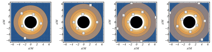
Figure 1: The shape of the scalar field $\Phi(r,\theta)$ described by the equation (31) in $x-z$ plane for the different values of $\gamma_{*}$ parameter: $\gamma_{*}=0.9$, $\gamma_{*}=1$, $\gamma_{*}=1.1$ and $\gamma_{*}=1.2$.

III.1 Energy conditions

In this subsection we briefly study energy condition in the spacetime of the generalized $\gamma$-metric given in the equation (30). The energy-momentum tensor for the scalar field can be expressed as

$$T_{\mu\nu}=\epsilon\left(\partial_{\mu}\Phi\partial_{\nu}\Phi-\frac{1}{2}g_{\mu\nu}g^{\alpha\beta}\partial_{\alpha}\Phi\partial_{\beta}\Phi\right)\ ,$$ (32)

from the expression (32) the energy density and the components of the pressure can be defined as $\rho=T_{0}^{0}$ and $P_{i}=T_{i}^{i}$, and the explicit form of the energy density and the components of the pressure is

$$\rho=P_{\theta}=P_{\phi}=-P_{r} = -\frac{\epsilon\gamma_{*}^{2}M^{2}}{2r^{4}}\left(1-\frac{2M}{r}\right)^{\gamma-2}\left(1-\frac{M^{2}\sin^{2}\theta}{r^{2}-2Mr}\right)^{\gamma^{2}+\epsilon\gamma_{*}^{2}-1}\ .$$

The null energy condition (NEC) can be found from the expression $\rho+P_{i}\geq 0$ ($i=r,\theta,\phi$), using the equation (III.1) as

$$\rho+P_{r} \equiv 0\ ,$$ (33)

$$\rho+P_{\theta} = \rho+P_{\phi}=-\frac{\epsilon\gamma_{*}^{2}M^{2}}{r^{4}}\left(1-\frac{2M}{r}\right)^{\gamma-2}\left(1-\frac{M^{2}\sin^{2}\theta}{r^{2}-2Mr}\right)^{\gamma^{2}+\epsilon\gamma_{*}^{2}-1}\ .$$ (34)

The physical interpretation of NEC is that the energy density measured by an observer traversing along null curve is always positive (never negative). One can see that the expression (33) is always satisfied by the NEC condition for the spacetime metric (30) while the expression (34) satisfies the NEC condition only in the case when $\epsilon\leq 0$ which corresponds to the phantom field. This means that the observer traversing along null curve can measure positive energy even in the case of the antigravitating phantom scalar field. Figure 2 shows the NEC precisely where the radial dependence of $\rho+P_{i}$ ($i=r,\theta,\phi$).

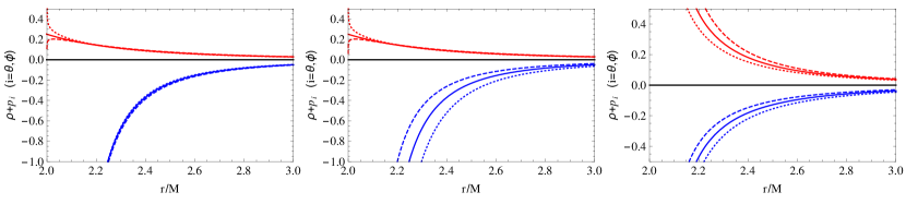
Figure 2: Radial dependence of $\{\rho+P_{i}\}$ ($i=r,\theta,\phi$) for the different values of the parameters $\gamma$ and $\gamma_{*}$. (Left panel) Solid line corresponds to $\gamma=1$, dashed line to $\gamma=0.9$ and dashed line to $\gamma=1.1$ at $\gamma_{*}=1$ and $\theta=\pi/2$. (Central panel) Solid line corresponds to $\gamma_{*}=1$, dashed line to $\gamma_{*}=0.9$ and dashed line to $\gamma_{*}=1.1$ at $\gamma=1$ and $\theta=\pi/2$. (Right panel) Solid line corresponds to $\gamma=1$, dashed line to $\gamma=0.9$ and dashed line to $\gamma=1.1$ at $\gamma_{*}=1$ and $\theta=0$.

III.2 Test particle motion

In this subsection we study test particle motion in the spacetime metric (30). The Hamiltonian for test particle with mass $m$ can be written in the form Kološ et al. (2015)

$$H=\frac{1}{2}g^{\mu\nu}p_{\mu}p_{\nu}+\frac{1}{2}\,m^{2}\ ,$$ (35)

where $p^{\mu}=mu^{\mu}$ is the kinematical four-momentum. The equations for particle motion are

$$\frac{dx^{\mu}}{d\zeta}\equiv p^{\mu}=\frac{\partial H}{\partial p_{\mu}}\ ,\qquad\frac{dp_{\mu}}{d\zeta}=-\frac{\partial H}{\partial x^{\mu}}\ .$$ (36)

Here the affine parameter $\zeta$ of the particle is related to its proper time $\tau$ by the relation $\zeta=\tau/m$.

Because of the symmetries of the modified $\gamma$-metric spacetime (30) one can easily find the conserved quantities that are the energy and the axial angular momentum of the particle and can be expressed as

$$E = -p_{t}=mg_{tt}\frac{dt}{d\tau}\ ,$$ (37)

$$L = p_{\phi}=mg_{\phi\phi}\frac{d\phi}{d\tau}\ .$$ (38)

Introducing for convenience the specific parameters, energy ${\cal E}$ and axial angular momentum ${\cal L}$

$${\cal E}=\frac{E}{m}\ ,\quad{\cal L}=\frac{L}{m}\ ,$$ (39)

one can rewrite the Hamiltonian (35) in the form

$$H=\frac{1}{2}g^{rr}p_{r}^{2}+\frac{1}{2}g^{\theta\theta}p_{\theta}^{2}+\frac{m^{2}}{2}g^{tt}\left[{\cal E}^{2}-V_{\rm eff}(r,\theta)\right]\ ,$$ (40)

where $V_{\rm eff}(r,\theta)$ denotes the effective potential of the test particle which is given by the relation

$$V_{\rm eff}(r,\theta) \equiv -g_{tt}\left(1+g^{\phi\phi}{\cal L}^{2}\right)$$

$$= \left(1-\frac{2M}{r}\right)^{\gamma}\left[1+\frac{{\cal L}^{2}}{r^{2}\sin^{2}\theta}\left(1-\frac{2M}{r}\right)^{\gamma-1}\right]\ .$$

It is important to note, that the effective potential $V_{\rm eff}(r,\theta)$ depends only on the metric parameter $\gamma$ while it is free of the parameters $\epsilon$ and $\gamma_{*}$.

The particle motion is limited by the energetic boundaries given by

$${\cal E}^{2}=V_{\rm eff}(r,\theta)\ .$$ (42)

Now we properly investigate the features of the effective potential (III.2) represented in Fig. 3. The stationary points of the effective potential $V_{\rm eff}(r,\theta)$ function, where maxima or minima can exist, are given by the equations

$$\partial_{r}V_{\rm eff}(r,\theta)=0\ ,\qquad\partial_{\theta}V_{\rm eff}(r,\theta)=0\ .$$ (43)

The second of the extrema equations (43) gives $\theta=\pi/2$. In other words, all extrema of the $V_{\rm eff}(r,\theta)$ function are located at the equatorial plane and there is no off-equatorial extrema. The first extrema equation of (43) leads to equation being quadratic with respect to the specific angular momentum ${\cal L}$ and hence the circular orbits can be determined by the relation Chowdhury et al. (2012)

$${\cal L}^{2}={\cal L}_{\rm ext}^{2}(r)\equiv\frac{\gamma Mr^{2}}{r-M(1+2\gamma)}\left(1-\frac{2M}{r}\right)^{1-\gamma}\ .$$ (44)

At Fig. 4 the function ${\cal L}_{\rm ext}(r)$ is plotted for various values of parameter $\gamma$. Similarly, the energy of the test particle can be expressed as

$${\cal E}^{2}={\cal E}_{\rm ext}^{2}(r)\equiv\frac{r-M(1+\gamma)}{r-M(1+2\gamma)}\left(1-\frac{2M}{r}\right)^{\gamma}\ .$$ (45)

The local extrema of ${\cal L}_{\rm ext}(r)$ function is equivalent to $\partial^{2}_{r}V_{\rm eff}(r,\theta=\pi/2)=0$ condition and they determine the innermost stable circular orbits (ISCO) radius located at

$$r_{\rm ISCO}/M=1+3\gamma+\sqrt{5\gamma^{2}-1}\ ,$$ (46)

and from equation (46) we can find that $\gamma$ parameter should be $\gamma\geq 1/\sqrt{5}$.

The unstable circular photon orbit $m=0$ given by the divergence of the effective potential (III.2) will be located at

$$r_{\rm ph}/M=1+2\gamma\ .$$ (47)

In the case when $\gamma=1$ one can have $r_{\rm ISCO}=6M$ and $r_{\rm ph}=3M$ which are responsible for the radius of the ISCO and photon sphere, respectively, in the Schwarzschild spacetime.

In Fig. 4 the various dependences of the radius of the ISCO and the photon sphere are shown. In the range of the values of the $\gamma\geq 1$ one can see that with increasing the $\gamma$ parameter the radius of ISCO and photon sphere increase while in the range of the values $1/\sqrt{5}\leq\gamma\leq 1$ they are small in comparison with that in general relativity.

One can easily see that the Eqs. (44), (45) and (46) for the angular momentum, the energy and radius of ISCO of the test particle, respectively, do not contain $q$ which means that the gravitating scalar field does not act on the test particles in the equatorial plane. Numerical calculations show that the effects of the gravitating scalar field can be seen in particle motion in off-equatorial plane. As a test of the spacetime geometry (30) we have presented the particle trajectories for the different values of the metric parameters $\gamma$, $\gamma_{*}$ and $\epsilon$ in several planes in Fig. 5.

Figure 3: Radial profiles of effective potential in equatorial plane $V_{\rm eff}(r,\pi/2)$ for the various values of angular momentum $L$. In the plots the different values for $\gamma$ parameter are used.

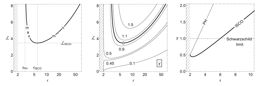
Figure 4: (Left panel) Position of extrema (max. min.) of the effective potential, giving stable (min) and unstable (max) circular orbits for the Schwarzschild ($\gamma=1$) spacetime. (Central panel) Position of extrema (max. min.) of effective potential for the different values of the $\gamma$ parameter. (Right panel) Position of the ISCO and photon orbit in the dependence from the parameter the $\gamma$.

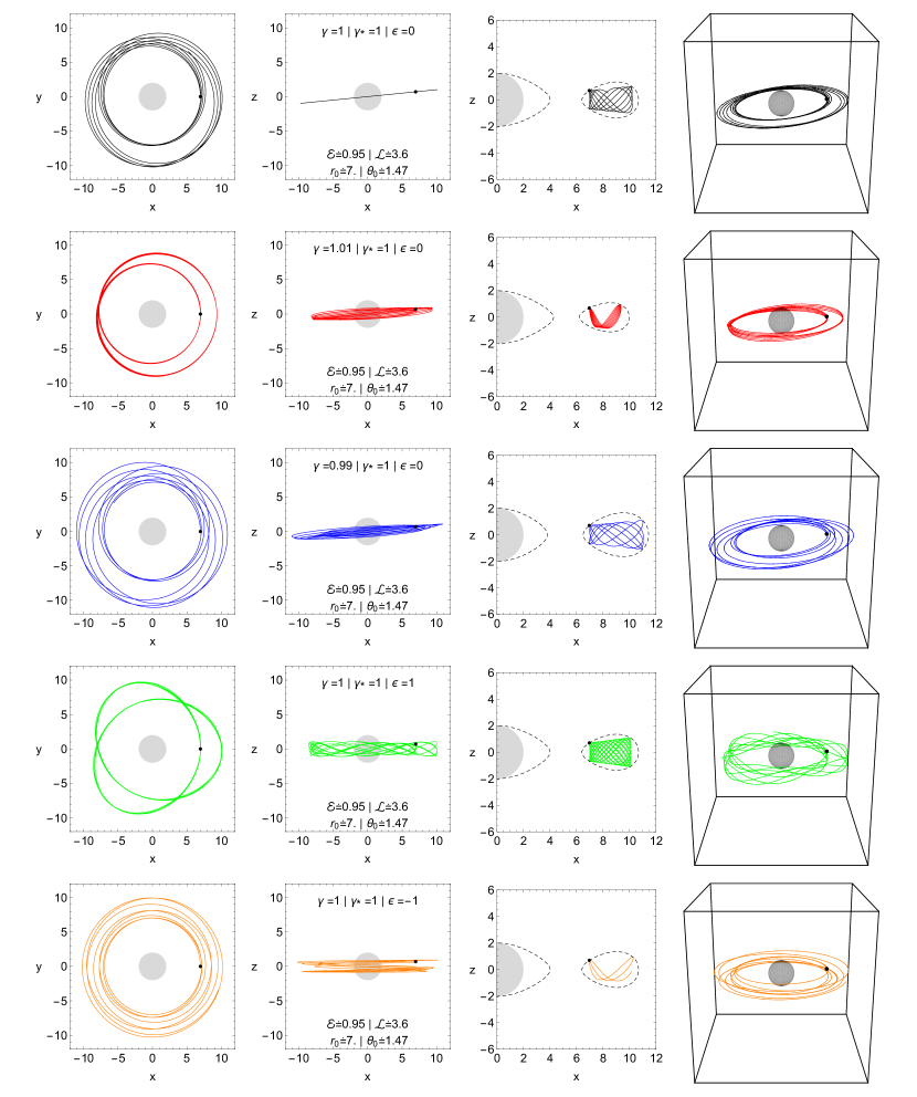
Figure 5: Test particle trajectories in the spacetime metric (30) for the different values of parameters $\gamma$, $\gamma_{*}$ and $\epsilon$. In first and second (including third) columns particle trajectories $x-y$ and $x-z$ planes are given while in the fourth column a 3D $x-y-z$ pattern of particle trajectory is shown.

IV Analytic solution of the Einstein equations with self-gravitating scalar field for the quadrupole-moment metric

In this section we briefly consider the influence of the gravitating scalar field into the quadrupole moment metric, which is described by Erez-Rosen (Erez and Rosen, 1959), with two free parameters of the black hole, mass $M$ and mass quadrupole moment $q$. Now we can consider the next leading order approximation in the coefficients $q_{l}$ and $p_{l}$ in the solutions (22)-(24) of the field equations. We study the case when $q_{0}=p_{0}=1$, $q_{1}=p_{1}=0$ (which is not existed of the mass dipole moment), and $q_{l}=p_{l}=0$ ($l>2$), and then we have

$$\Phi(X,Y) = \frac{1}{2}\ln\frac{X-1}{X+1}+\frac{q_{*}}{2}(3Y^{2}-1)\left(\frac{3X}{2}+\frac{3X^{2}-1}{4}\ln\frac{X-1}{X+1}\right)\ ,$$ (48)

$$U(X,Y) = \frac{1}{2}\ln\frac{X-1}{X+1}+\frac{q}{2}(3Y^{2}-1)\left(\frac{3X}{2}+\frac{3X^{2}-1}{4}\ln\frac{X-1}{X+1}\right)\ ,$$ (49)

$$V(X,Y) = \frac{(1+q)^{2}+\epsilon(1+q_{*})^{2}}{2}\ln\frac{X^{2}-1}{X^{2}-Y^{2}}-\frac{3(q+\epsilon q_{*})}{2}(1-Y^{2})\left(X\ln\frac{X-1}{X+1}+2\right)$$ (50)

$$+ \frac{9(q^{2}+\epsilon q_{*}^{2})}{16}(1-Y^{2})\Big{[}X^{2}+Y^{2}-9X^{2}Y^{2}-\frac{4}{3}+X\left(X^{2}+7Y^{2}-9X^{2}Y^{2}-\frac{5}{3}\right)\ln\frac{X^{2}-1}{X^{2}-Y^{2}}$$

$$+ \frac{1}{4}\left(X^{2}-1\right)\left(X^{2}+Y^{2}-9X^{2}Y^{2}-1\right)\ln^{2}\frac{X^{2}-1}{X^{2}-Y^{2}}\Big{]}\ ,$$

where $q$ and $q_{*}$ are the mass quadrupole moments of the gravitational object. The Erez-Rosen solution Erez and Rosen (1959) can be obtained in the limiting case when $q_{*}=0$. In order to find the physically meaningful solution for the scalar field one writes it in terms of the spherical coordinates in the form

$$\Phi(r,\theta) = \frac{1}{2}\ln\left(1-\frac{2M}{r}\right)+\frac{q_{*}}{2}\left[\frac{3r^{2}-6Mr+2M^{2}}{4M^{2}}\ln\left(1-\frac{2M}{r}\right)+\frac{3(r-M)}{2M}\right](3\cos^{2}\theta-1)\ ,$$ (51)

and in the weak field approximation the equation (51) has a form

$$\Phi(r,\theta)\simeq-\frac{M}{r}+\frac{q_{*}M^{3}}{15r^{3}}(3\cos^{2}\theta-1)\ .$$ (52)

We can see that the first linear term in the right hand side of the equation (52) is responsible for Newtonian potential, the second term is responsible for the quadrupole moment potential, where $q_{*}$ is dimensionless mass quadrupole moment produced by the gravitating scalar field.

In Fig.6 the equipotential surface of the scalar field $\Phi(r,\theta)$ using the expression (51) for the different values of the quadrupole moment $q_{*}$ is illustrated. One can easily see that due to the $q_{*}$ parameter the spacetime around the black hole is axially deformed.

It is a convenient to write simple analytical form of the metric for further calculations. In the linear approximation of the mass quadrupole moments $q$ and $q_{*}$, one can write the following spacetime metric

$$g_{tt} = -\left(1-\frac{2M}{r}\right)\Big{[}1+qF_{1}(r)P_{2}(\cos\theta)\Big{]}+{\cal O}(q^{2})\ ,$$ (53a)

$$g_{rr} = \left(1-\frac{2M}{r}\right)^{-1}\left(1+\frac{M^{2}\sin^{2}\theta}{r^{2}-2Mr}\right)^{-\epsilon}$$ (53b)

$$\times \left\{1+qF_{1}(r)P_{2}(\cos\theta)-(q+\epsilon q_{*})\left[2\ln\left(1+\frac{M^{2}\sin^{2}\theta}{r^{2}-2Mr}\right)+3F_{2}(r)\sin^{2}\theta\right]\right\}+{\cal O}(q^{2},q_{*}^{2})\ ,$$

$$g_{\theta\theta} = r^{2}\left(1+\frac{M^{2}\sin^{2}\theta}{r^{2}-2Mr}\right)^{-\epsilon}$$ (53c)

$$\times \left\{1+qF_{1}(r)P_{2}(\cos\theta)-(q+\epsilon q_{*})\left[2\ln\left(1+\frac{M^{2}\sin^{2}\theta}{r^{2}-2Mr}\right)+3F_{2}(r)\sin^{2}\theta\right]\right\}+{\cal O}(q^{2},q_{*}^{2})\ ,$$

$$g_{\phi\phi} = r^{2}\sin^{2}\theta\Big{[}1-qF_{1}(r)P_{2}(\cos\theta)\Big{]}+{\cal O}(q^{2})\ ,$$ (53d)

which is a generalized form of the Erez-Rosen metric with external parameter $q_{*}$ produced by the gravitational scalar field where $P_{2}(\cos\theta)=(3\cos^{2}\theta-1)/2$ and the functions $F_{1}(r)$ and $F_{2}(r)$ are defined as

$$F_{1}(r) = 3\left(\frac{r}{M}-1\right)+\left(\frac{3r^{2}}{2M^{2}}-\frac{3r}{M}+1\right)\ln\left(1-\frac{2M}{r}\right)\ ,$$ (54)

$$F_{2}(r) = 2+\left(\frac{r}{M}-1\right)\ln\left(1-\frac{2M}{r}\right)\ .$$ (55)

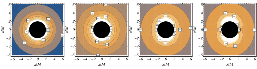
Figure 6: The equipotential surface of the scalar potential $\Phi(r,\theta)$ in $x-z$ plane for the different values of the mass quadrupole moment: $q_{*}=0$, $q_{*}=0.2$, $q_{*}=0.5$ and $q_{*}=1$.

IV.1 Test particle motion

Consider the particle motion in the spacetime metric (53) with the linear term of quadrupole momenta $q$ and $q_{*}$, Using the equation of motion for the test particle we can obtain the following effective potential

$$V_{\rm eff}(r)=\left(1-\frac{2M}{r}\right)\left[1+\frac{{\cal L}^{2}}{r^{2}}-\frac{qF_{1}(r)}{2}\left(1+\frac{2{\cal L}^{2}}{r^{2}}\right)\right]\ .$$ (56)

Figure 7 draws radial dependence of the effective potential for motion in the equatorial plane ($\theta=\pi/2$) for the different values of the angular momentum, and for three different values of quadruple moment $q$.

In order to find the critical values of the energy and the angular momentum one have to use the following conditions

$${\cal E}^{2}=V_{\rm eff}(r)\ ,\quad V_{\rm eff}^{\prime}(r)=0\ ,$$ (57)

and the solution of these equations for the energy and the angular momentum can be found as

$${\cal E}_{\rm ext}^{2} = \frac{(r-2M)^{2}}{r(r-3M)}-q\Bigg{[}\frac{(r-M)(r-2M)\left(6r^{2}-21Mr+19M^{2}\right)}{2Mr(r-3M)^{2}}$$ (58)

$$+\frac{(r-2M)^{2}\left(6r^{3}-21Mr^{2}+23M^{2}r-6M^{3}\right)}{4M^{2}r(r-3M)^{2}}\ln\left(1-\frac{2M}{r}\right)\Bigg{]}+{\cal O}\left(q^{2}\right)\ ,$$

$${\cal L}_{\rm ext}^{2} = \frac{Mr^{2}}{r-3M}-q\Bigg{[}\frac{r^{2}(r-M)\left(3r^{2}-9Mr+10M^{2}\right)}{2M(r-3M)^{2}}$$ (59)

$$+\frac{r^{2}\left(3r^{4}-15Mr^{3}+30M^{2}r^{2}-26M^{3}r+6M^{4}\right)}{4M^{2}(r-3M)^{2}}\ln\left(1-\frac{2M}{r}\right)\Bigg{]}+{\cal O}\left(q^{2}\right)\ .$$

The radius of ISCO can be found from the condition $V_{\rm eff}^{\prime\prime}(r)\leq 0$ in addition to expressions (58) and (59) which allow us to obtain the following nonlinear equation

$$r-6M-q\Bigg{[}\frac{12r^{5}-111Mr^{4}+364M^{2}r^{3}-501M^{3}r^{2}+214M^{4}r+54M^{5}}{2M^{2}(r-2M)(r-3M)}$$

$$+\frac{12r^{5}-99Mr^{4}+273M^{2}r^{3}-286M^{3}r^{2}+54M^{4}r+36M^{5}}{4M^{3}(r-3M)}\ln\left(1-\frac{2M}{r}\right)\Bigg{]}+{\cal O}\left(q^{2}\right)=0\ .$$ (60)

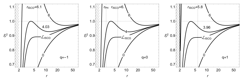
Figure 7: Radial profiles of effective potential in equatorial plane $V_{\rm eff}(r,\pi/2)$ for the various values of angular momentum $L$. In the plots the different values for $q$ parameter are used.

Obviously, it is difficult to get analytical solution of the equation (IV.1). Hereafter performing a careful numerical analysis of expression (IV.1), one can find that the radius of the ISCO decreases with increasing of the value of $q$ parameter. In Table 1 a list of numerical solutions for the radius of ISCO, the energy and the angular momentum of particles for different values of the mass quadrupole moment is shown. With the increase of the parameter $q$ radius of the ISCO to a gravitational object, the values of the energy and the angular momentum of particles decrease. It means that the mass quadrupole moment $q$ sustain stability of particles circularly orbiting around the black hole. One can conclude that due to the mass quadrupole moment of the black hole particles motion is more stable than that in the Schwarzschild spacetime.

Table 1: Dependence of the mass quadrupole moment $q$ from the values of the radius of ISCO ($r_{\rm ISCO}$), the critical energy (${\cal E}_{\rm ISCO}$) and angular momentum (${\cal L}_{\rm ISCO}$) of the the test particles orbiting around the black hole.

$q$	${r_{\rm ISCO}}/M$	${\cal L}_{\rm ISCO}/M$	${\cal E}_{\rm ISCO}$
0	6.00000	3.46410	0.888889
0.1	5.98552	3.46155	0.888684
0.2	5.97090	3.45898	0.888478
0.3	5.95616	3.45640	0.888269
0.4	5.94127	3.45379	0.888057
0.5	5.92624	3.45116	0.887844
0.6	5.91107	3.44852	0.887627
0.7	5.89575	3.44585	0.887408
0.8	5.88027	3.44316	0.887187
0.9	5.86464	3.44046	0.886963
1.0	5.84884	3.43773	0.886736

The trajectories of the test particles in the spacetime of the generalized Erez-Rosen metric (53) at the several planes for the different values of the parameters are shown in Fig. 8. The motion of the test particle becomes regular (not chaotic as in the Kerr spacetime) in the quadrupole moment metric.

It is interesting to study chaotic motion in the spacetime with deformation parameters $\gamma$, $\gamma_{*}$, $q$ and $q_{*}$. In order to check chaotic motion around the black hole we have used the general form of the spacetime metric which is given by the expressions (48)-(50). Numerical calculations show that the trajectory of test particles become chaotic for large values of the $\gamma_{*}$, $q$, and $q_{*}$ parameters, as shown in Fig. 9.

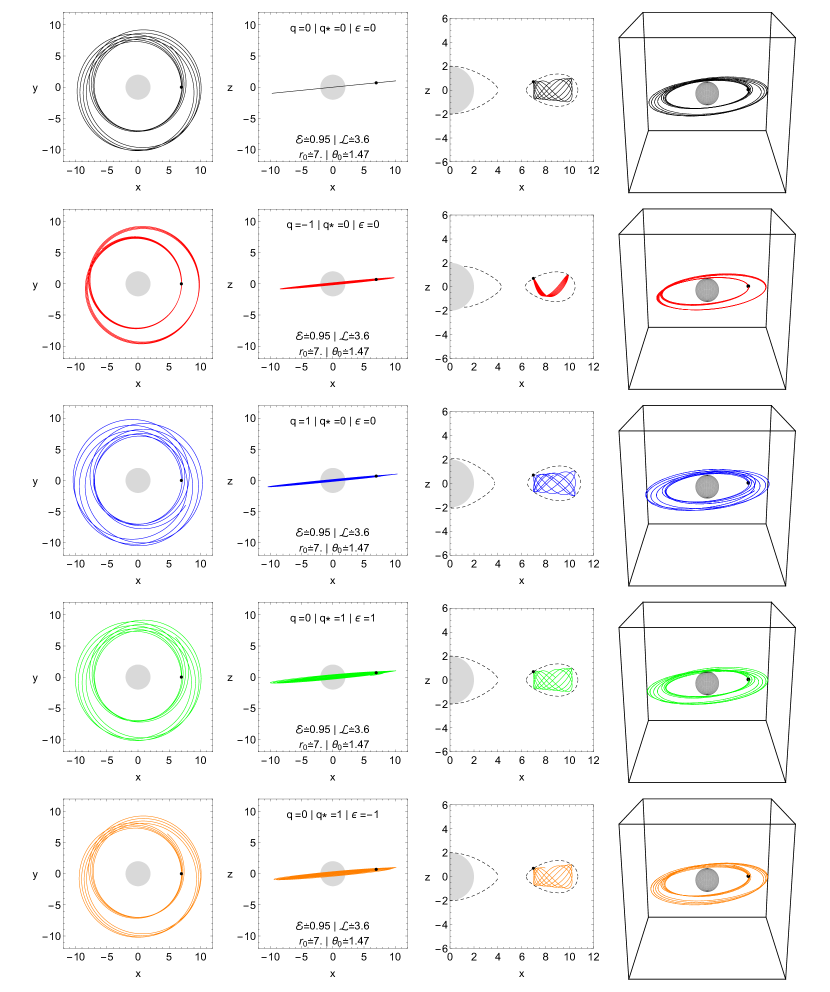
Figure 8: Test particle trajectories in the spacetime metric (53) for the different values of parameters $q$, $q_{*}$ and $\epsilon$. In first and second (including third) columns particle trajectories in $x-y$ and $x-z$ planes are given, respectively, while in the fourth column 3D $x-y-z$ pattern of particle trajectory is shown.

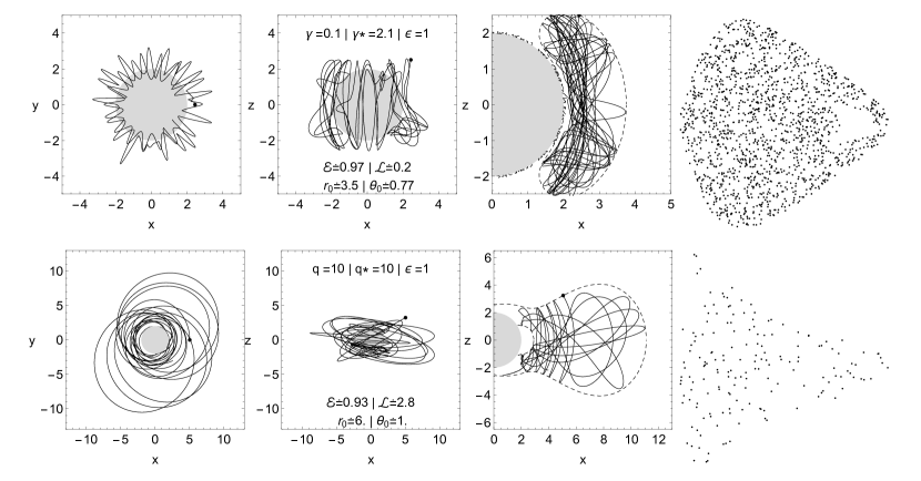
Figure 9: Chaotic trajectories of test particle in several planes in background geometry decribed by (30) and (53) when $\epsilon=1$. In first and second (including third) columns particle trajectories $x-y$ and $x-z$ planes are given while in the fourth column phase-space diagram of particle trajectory is shown.

IV.2 Energy conditions

Using the expression for the energy-momentum (32) one can easily find the density and the components of the pressure for scalar field defined in equation (51) in the form

$$\rho = P_{\theta}=P_{\phi}=-P_{r}$$ (61)

$$= -\frac{\epsilon M^{2}}{2r^{3}(r-2M)}\left(1+\frac{M^{2}\sin^{2}\theta}{r(r-2M)}\right)^{\epsilon}\Bigg{\{}1+q\left[2\ln\left(1+\frac{M^{2}\sin^{2}\theta}{r(r-2M)}\right)-F_{1}(r)P_{2}(\cos\theta)+3F_{2}(r)\sin^{2}\theta\right]$$

$$+ q_{*}\left[2\epsilon\ln\left(1+\frac{M^{2}\sin^{2}\theta}{r(r-2M)}\right)+3\epsilon F_{2}(r)\sin^{2}\theta+1-\frac{6r}{M}+\frac{3r^{2}}{M^{2}}+\frac{3r}{2M}\left(\frac{r}{M}-2\right)\left(\frac{r}{M}-1\right)\ln\left(1-\frac{2M}{r}\right)\right]\Bigg{\}}\ ,$$

from equation (61) we can see that $\rho+P_{r}=0$ which always satisfies the NEC condition while the expressions for $\rho+P_{\theta,\phi}$ satisfy the NEC condition only in the case when $\epsilon\leq 0$ which corresponds to the phantom field.

V Conclusion

In the present paper we have derived axisymmetric and static solutions of the Einstein field equations by taking into account the effect of an additional self-gravitating scalar field. In particular we have presented an exact analytical solution of the combined Einstein equations for two different modified spacetime metrics which belong to the Weyl class of solutions as (i) the modified $\gamma$-metric and (ii) the modified quadrupole moment metric. Obtained results can be summarized as follows:

• We have studied the influence of the scalar field in spacetime properties of axial-symmetric and static vacuum solutions of combined Einstein field equations which generalize the Schwarzschild’s spherically symmetric solution to include $\gamma$, $\gamma_{*}$ and mass quadrupole parameters $q$, $q_{*}$. We have required that the scalar field is axially symmetric, static and that the solutions satisfy the asymptotic flatness and curvature regularity. We have obtained a generalized form of the $\gamma$ metric with additional the $\gamma_{*}$ and generalized form of the Eres-Rosen (quadrupole moment) metric which includes $q_{*}$ mass quadrupole produced by the self-gravitating scalar field.

• The analytical expressions for the components of the energy-momentum tensor are obtained for the self-gravitating scalar field. Extensive analysis of the energy of scalar field has shown that in the case of phantom field ($\epsilon=-1$) it satisfies the NEC while in the case of gravitating scalar field ($\epsilon=1$) it does not satisfy the NEC.

• We have studied the test particle motion in the spacetime of both generalized the $\gamma$-metric and the quadrupole moment metric and have probed $\gamma_{*}$ and $q_{*}$ parameters produced by the gravitating scalar field into the test particle motion. The Hamilton-Jacobi equation of motion for the test particle is chosen as in our preceding research done in Ref. Kološ et al. (2015). Our analysis shows that $\gamma_{*}$ and $q_{*}$ parameters do not contribute into the energy and angular momentum of the test particle and consequently do not affect particle trajectory at the equatorial plane. Consequently, the motion of the test particle becomes regular (rather than chaotic) in both generalized $\gamma$ and generalized Erez-Rosen metrics.

• We have presented the exact analytical expression for the radius of the ISCO, the critical values of the energy and the angular momentum of the test particles in terms of the $\gamma$ parameter in the spacetime of the $\gamma$-metric. It is shown that for the range $\gamma\geq 1/\sqrt{5}$ of the values of the $\gamma$ parameter the radius of ISCO and the photon sphere increase. For the range of the values of the $\gamma\geq 1$ we have found that with increasing the $\gamma$ parameter the radius of ISCO and photon sphere increase while for the range of the values $1/\sqrt{5}\leq\gamma\leq 1$ they are small in comparison with that in the Schwarzschild spacetime. After performing numerical analysis of the equations of particle motion in the spacetime of the generalized quadrupole moment metric we have found that the radius of ISCO decreases with an increase of the value of the $q$ parameter. It has been shown that the quadrupole moment metric has circular orbits that are more strongly bounded when compared to that in the Schwarzschild metric.

VI acknowledgments

The research of B.A. and B.T. is partially supported by Grants No. VA- FA-F-2-008 and No. YFA-Ftech-2018-8 of the Uzbekistan Ministry for Innovation Development, and by the Abdus Salam International Centre for Theoretical Physics through Grant No. OEA-NT-01. B.A. would like to acknowledge the support of the German Academic Exchange Service DAAD for supporting his stay at Frankfurt University. M.K. acknowledges the Czech Science Foundation under the Grant No. 16-03564Y. Z.S. acknowledges the Albert Einstein Centre for Gravitational and Astrophysics supported under the Czech Science Foundation under the Grant No. 14-37086G. The authors would like to thank Professor H. Quevedo for pointing out the methods of derivation of new solutions of the Einstein equations and Professor Y. M. Cho for suggesting we include the scalar field in the solutions. B.A. acknowledges the support from Nazarbayev University Faculty Development Competitive Research Grants: “Quantum gravity from outer space and the search for new extreme astrophysical phenomena”, Grant No. 090118FD5348.

Appendix A The function $V(X,Y)$

The explicit form of the function $V(X,Y)$ in the equation (24) is given by Quevedo (1989)

$$V(X,Y)=\sum_{l,n=0}^{\infty}(-1)^{l+n}(q_{l}q_{n}+\epsilon p_{l}p_{n})\Gamma^{\{ln\}}\ ,$$ (62)

where

$$\Gamma^{\{ln\}} = \frac{1}{2}\ln\frac{X^{2}-1}{X^{2}-Y^{2}}+\left(\epsilon_{n}+\epsilon_{l}-2\epsilon_{n}\epsilon_{l}\right)\ln\frac{X+1}{X-1}$$

$$+ (X^{2}-1)\Big{[}X\Big{(}A_{n,l}Q_{n}^{\prime}(X)Q_{l}(X)+A_{l,n}Q_{l}^{\prime}(X)Q_{n}(X)\Big{)}-C_{n,l}Q_{n}(X)Q_{l}(X)\Big{]}$$

$$+ (X^{2}-1)\left[(1-\epsilon_{n}){\cal C}_{l}+\epsilon_{l}{\cal C}_{l+1}-\frac{\epsilon_{n}}{l+1}\Big{(}P_{l}(Y)-(-1)^{l}\Big{)}Q_{l}^{\prime}(X)\right]$$

$$+ (X^{2}-1)^{2}\Big{[}Q_{l}(X){\cal B}_{l,n}-Q_{l}^{\prime}(X){\cal A}_{l,n}+\frac{1}{n+1}A_{l,n}Q_{l}^{\prime}(X)Q_{n}^{\prime}(X)\Big{]}\ ,$$

with

$$\epsilon_{n}=\left\{\begin{array}[]{lcr}1\ ,\quad{\rm n=even\,\,integer}\ ,\\ \\ 0\ ,\quad{\rm n=odd\,\,integer}\ ,\end{array}\right.$$

and

$${\cal A}_{l,n} = \sum_{k=0}^{[n/2-1]}\left(\frac{1}{n-2k+1}+\frac{1}{n-2k}\right)A_{l,n-2k}Q_{n-2k}^{\prime}(X)\ ,$$ (63)

$${\cal B}_{l,n} = \sum_{k=0}^{[n/2-1]}\left(\frac{1}{n-2k-1}+\frac{1}{n-2k}\right)B_{l,n-2k-1}Q_{n-2k-1}^{\prime}(X)\ ,$$ (64)

$${\cal C}_{l,n} = \sum_{k=0}^{[n/2-1]}\left(\frac{1}{n-2k-1}+\frac{1}{n-2k}\right)\left[P_{n-2k-1}+(-1)^{n+1}\right]Q_{n-2k-1}^{\prime}(X)\ ,$$ (65)

$$A_{l,n} = \sum_{k=0}^{[n/2-1]}\sum_{s=0}^{\mu(n,l-2k-1)}\frac{(2l-4k-1)K(l-2k-1,n,l)}{2(l+n)-4(k+s)-1}\left(P_{l+n-2(k+s)}(Y)-P_{l+n-2(k+s+1)}(Y)\right)\ ,$$ (66)

$$B_{l,n} = \sum_{j=0}^{[n/2-1]}\sum_{k=0}^{[n/2-1]}\sum_{s=0}^{\mu(n-2k-1,l-2j-1)}\frac{(2l-4j-1)(2n-4k-1)K(l-2j-1,n-2k-1,s)}{2(l+n)-4(j+k+s)-3}$$

$$\times \left(P_{l+n-2(j+k+s)-1}(Y)-P_{l+n-2(k+l+s)-3}(Y)\right)\ ,$$

$$C_{l,n} = B_{n+1,l}-(n+1)A_{n,l}\ ,$$ (68)

here a bracket $[Q]$ denotes an integer part of quantity $Q$ and $\mu(a,b)={\rm min}(a,b)$, the Clebsch-Gordon coefficients $K(l,n,k)$ are defined by

$$K(l,n,k)=\frac{2l+2n-4k+1}{2l+2n-2k+1}\frac{a_{l-k}a_{n-k}}{a_{l+n-k}}\ ,$$ (69)

and

$$a_{k}=\frac{(2k-1)!!}{k!}\ .$$

References

- Tolman (1939) R. C. Tolman, Physical Review 55, 364 (1939).
- Hartle (1967) J. B. Hartle, Astrophys. J. 150, 1005 (1967).
- Hartle and Thorne (1968) J. B. Hartle and K. S. Thorne, Astrophys. J. 153, 807 (1968).
- Hartle and Thorne (1969) J. B. Hartle and K. S. Thorne, Astrophys. J. 158, 719 (1969).
- Stephani et al. (2003) H. Stephani, D. Kramer, M. MacCallum, C. Hoenselaers, and E. Herlt, Exact solutions of Einstein’s field equations, 2nd ed. by Hans Stephani, Dietrich Kramer, Malcolm MacCallum, Cornelius Hoenselaers, and Eduard Herlt. Cambridge monographs on mathematical physics. Cambridge, UK: Cambridge University Press, 2003 (2003).
- D. Kramer and Herlt (1980) M. M. D. Kramer, H. Stephani and E. Herlt, Exact Solutions of Einstein’s Field Equations (Cambridge University Press, Cambridge, 1980).
- Erez and Rosen (1959) G. Erez and N. Rosen, Bull. Res. Counc. Isr. 8 (1959).
- Janis et al. (1968) A. I. Janis, E. T. Newman, and J. Winicour, Physical Review Letters 20, 878 (1968).
- Voorhees (1970) B. H. Voorhees, Phys. Rev. D 2, 2119 (1970).
- Gutsunayev et al. (1985) T. I. Gutsunayev, T. I. Gutsunaev, and V. S. Manko, General Relativity and Gravitation 17, 1025 (1985).
- Quevedo and Mashhoon (1985) H. Quevedo and B. Mashhoon, Physics Letters A 109, 13 (1985).
- Quevedo (1986) H. Quevedo, Phys.Rev. D 33, 324 (1986).
- Quevedo (1987) H. Quevedo, General Relativity and Gravitation 19, 1013 (1987).
- Quevedo (1989) H. Quevedo, Phys.Rev. D 39, 2904 (1989).
- Gutsunaev and Manko (1989) T. I. Gutsunaev and V. S. Manko, Phys. Rev. D 40, 2140 (1989).
- Quevedo and Mashhoon (1990) H. Quevedo and B. Mashhoon, Physics Letters A 148, 149 (1990).
- Quevedo (1991) H. Quevedo, Physical Review Letters 67, 1050 (1991).
- Frutos-Alfaro et al. (2018) F. Frutos-Alfaro, H. Quevedo, and P. A. Sanchez, Royal Society Open Science 5, 170826 (2018), arXiv:1704.06734 [gr-qc] .
- Boshkayev et al. (2016) K. Boshkayev, H. Quevedo, S. Toktarbay, B. Zhami, and M. Abishev, Gravitation and Cosmology 22, 305 (2016), arXiv:1510.02035 [gr-qc] .
- Contopoulos et al. (2016) I. G. Contopoulos, F. P. Esposito, K. Kleidis, D. B. Papadopoulos, and L. Witten, International Journal of Modern Physics D 25, 1650022 (2016), arXiv:1501.03968 [gr-qc] .
- Chowdhury et al. (2012) A. N. Chowdhury, M. Patil, D. Malafarina, and P. S. Joshi, Phys.Rev. D 85, 104031 (2012), arXiv:1112.2522 [gr-qc] .
- Quevedo and Parkes (1989) H. Quevedo and L. Parkes, General Relativity and Gravitation 21, 1047 (1989).
- Staykov et al. (2018) K. V. Staykov, D. Popchev, D. D. Doneva, and S. S. Yazadjiev, ArXiv e-prints (2018), arXiv:1805.07818 [gr-qc] .
- Gibbons and Volkov (2017) G. W. Gibbons and M. S. Volkov, Journal of Cosmology and Astroparticle Physics 5, 039 (2017), arXiv:1701.05533 [hep-th] .
- Fan and Lü (2015) Z.-Y. Fan and H. Lü, Phys. Rev. D 92, 064008 (2015), arXiv:1505.03557 [hep-th] .
- Fan and Lu (2015) Z.-Y. Fan and H. Lu, ArXiv e-prints (2015), arXiv:1507.04369 [hep-th] .
- Fan and Lü (2015a) Z.-Y. Fan and H. Lü, Physics Letters B 743, 290 (2015a), arXiv:1501.01727 [hep-th] .
- Fan and Lü (2015b) Z.-Y. Fan and H. Lü, Journal of High Energy Physics 4, 139 (2015b), arXiv:1501.05318 [hep-th] .
- Virbhadra (1997) K. S. Virbhadra, International Journal of Modern Physics A 12, 4831 (1997), gr-qc/9701021 .
- Dadhich and Banerjee (2001) N. Dadhich and N. Banerjee, Modern Physics Letters A 16, 1193 (2001), hep-th/0012015 .
- Herrera et al. (2005) L. Herrera, G. Magli, and D. Malafarina, General Relativity and Gravitation 37, 1371 (2005), gr-qc/0407037 .
- Herdeiro and Radu (2015) C. A. R. Herdeiro and E. Radu, International Journal of Modern Physics D 24, 1542014-219 (2015), arXiv:1504.08209 [gr-qc] .
- Erices and Martínez (2015) C. Erices and C. Martínez, Phys.Rev. D 92, 044051 (2015), arXiv:1504.06321 [gr-qc] .
- Sen (1992) A. Sen, Physical Review Letters 69, 1006 (1992), hep-th/9204046 .
- Toshmatov et al. (2014) B. Toshmatov, B. Ahmedov, A. Abdujabbarov, and Z. Stuchlik, Phys.Rev. D 89, 104017 (2014), arXiv:1404.6443 [gr-qc] .
- Toshmatov et al. (2017) B. Toshmatov, Z. Stuchlík, and B. Ahmedov, European Physical Journal Plus 132, 98 (2017).
- Kološ et al. (2015) M. Kološ, Z. Stuchlík, and A. Tursunov, Classical and Quantum Gravity 32, 165009 (2015), arXiv:1506.06799 [gr-qc] .