GLAD: GLocalized Anomaly Detection via Human-in-the-Loop Learning

Abstract

Human analysts that use anomaly detection systems in practice want to retain the use of simple and explainable global anomaly detectors. In this paper, we propose a novel human-in-the-loop learning algorithm called GLAD (GLocalized Anomaly Detection) that supports global anomaly detectors. GLAD automatically learns their local relevance to specific data instances using label feedback from human analysts. The key idea is to place a uniform prior on the relevance of each member of the anomaly detection ensemble over the input feature space via a neural network trained on unlabeled instances. Subsequently, weights of the neural network are tuned to adjust the local relevance of each ensemble member using all labeled instances. GLAD also provides explanations which can improve the understanding of end-users about anomalies. Our experiments on synthetic and real-world data show the effectiveness of GLAD in learning the local relevance of ensemble members and discovering anomalies via label feedback.

1 Introduction

Definition 1 (Glocal)

Reflecting or characterized by both local and global considerations.

End-users find it easier to trust algorithms they understand and are familiar with. Such algorithms are typically built on broadly general and simplifying assumptions over the entire feature space (i.e., global behavior), which may not be applicable universally (i.e., not relevant locally in some parts of the feature space) in an application domain. This observation is true of most machine learning algorithms including those for anomaly detection. We propose a principled technique referred as GLocalized Anomaly Detection (GLAD) which allows a human analyst to continue using anomaly detection ensembles with global behavior by learning their local relevance in different parts of the feature space via label feedback.

Ensembles of anomaly detectors often outperform single detectors (Aggarwal & Sathe, 2017). Additionally, anomalous instances can be discovered faster when the ensembles are used in conjunction with active learning, where a human analyst labels the queried instance(s) as nominal or anomaly (Veeramachaneni et al., 2016; Das et al., 2016, 2018; Siddiqui et al., 2018). A majority of the active learning techniques for discovering anomalies employ a weighted linear combination of the anomaly scores from the ensemble members. This approach works well when the members are themselves highly localized, such as the leaf nodes of tree-based detectors (Das et al., 2018). However, when the members of the ensemble are global (such as LODA projections (Pevny, 2015)), it is highly likely that individual detectors are incorrect in at least some local parts of the input feature space.

To overcome this drawback, our GLAD algorithm automatically learns the local relevance of each ensemble member in the feature space via a neural network using the label feedback from a human analyst. One interesting observation related to the key insight behind active learning with tree-based models (Tree-AAD) (Das et al., 2018) and GLAD is as follows: uniform prior over weights of each subspace (leaf node) in Tree-AAD and uniform prior over input feature space for the relevance of each ensemble member in GLAD are highly beneficial for label-efficient active learning. We can consider GLAD as very similar to the Tree-AAD approach. Tree-AAD partitions the input feature space into discrete subspaces and then places a uniform prior over those subspaces (i.e., the uniform weight vector to combine ensemble scores). If we take this view to an extreme by imagining that each instance in feature space represents a subspace, we can see the connection to GLAD. While Tree-AAD assigns the scores of discrete subspaces to instances (e.g., node depths for Isolation Forest), the scores assigned by GLAD are continuous, defined by the global ensemble members. The relevance in GLAD is analogous to the learned weights in Tree-AAD.

Our GLAD technique is similar in spirit to dynamic ensemble weighting (Jimenez, 1998). However, since we are in an active learning setting for anomaly detection, we need to consider two important aspects: (a) Number of labeled examples is very small (possibly none), and (b) To reduce the effort of the human analyst, the algorithm needs to be primed so that the likelihood of discovering anomalies is very high from the first feedback iteration itself. Specifically, we employ a neural network to predict the local relevance of each ensemble member. This network is primed with unlabeled data such that it places a uniform prior for the relevance of each ensemble member over the input feature space. In each iteration of the active learning loop, we select one unlabeled instance for querying, and update the weights of the neural network to adjust the local relevance of each ensemble member based on all the labeled instances. Our code and datasets are publicly available at https://github.com/shubhomoydas/ad_examples.

2 Related Work

Anomaly detection approaches are mostly unsupervised. It assumes that the concept of nominal and anomaly can be derived from the dataset. (Schölkopf et al., 2001; Breunig et al., 2000; Liu et al., 2008; Pevny, 2015; Emmott et al., 2015) are some of the classical algorithms for anomaly detection. One major problem of such approaches is the were not designed to incorporate feedbacks. And that introduced a lot of false alarms from the model. Inherent bias was the problem for such high false alarms. Ensemble based approaches were proposed to improve the performance (Aggarwal & Sathe, 2017). Some other variants are heterogeneous detectors (Senator et al., 2013), GMM (Emmott et al., 2015). The state of the art anomaly detection approach (Liu et al., 2008) is also an ensemble based approach.

For supervised and semi-supervised anomaly detection main assumptions are the presence of labels. And semi-supervised approaches like (Muñoz-Marí et al., 2010; Blanchard et al., 2010) was developed on an assumption that labels for nominals are only present. Later, (Görnitz et al., 2013) considers a semi-supervised algorithm for anomaly detection and employs active learning. Besides, there were some clustering assumptions made at (Zhu, 2005; Chapelle et al., 2009) for semi supervised settings. This assumption breaks when the problems is being applied for anomaly detection as the anomalies usually do not produce clusters in the data space.

Active learning based approaches for anomaly detection is becoming an important research area (Das et al., 2017; Siddiqui et al., 2018; Das et al., 2020; Veeramachaneni et al., 2016; Das et al., 2016; Guha et al., 2016; Nissim et al., 2014; Stokes et al., 2008; He & Carbonell, 2008; Almgren & Jonsson, 2004; Abe et al., 2006). To deploy anomaly detection systems in real-world this is a necessity for end user. It enables domain experts to interact with the system and update the model.

Explainability is an essential component for any learning based model (Doshi-Velez & Kim, 2017). The main objective of explainability is to help humans(end-users) understanding about the model and tools. Previous studies focused on ruleset based also known as disjunctive normal form (DNF) based explanatations. Simplicity of such models made them easily accessible for humans (Letham et al., 2015; Goh & Rudin, 2014; Fürnkranz et al., 2012). Another direction for explainabiltiy is to develop a model-agnostic mechanism. Some notable works are LIME (Ribeiro et al., 2016), Anchors (Ribeiro et al., 2018), and x-PACS (Macha & Akoglu, 2018) where they provide explanations for any pretrained model. For GLAD, model-agnostic techniques can be applied for generic ensembles. GLAD first identifies the most relevant ensemble member for an anomaly instance. Subsequently, the model-agnostic techniques can be employed to explain or describe the predictions of that detector.

3 Problem Setup

We will denote the input feature space by $\mathcal{X}\subseteq\mathbb{R}^{d}$. We are given a dataset ${\bf D}=\{{\bf x}_{1},...,{\bf x}_{n}\}$, where ${\bf x}_{i}\in\mathcal{X}$ is a data instance that is associated with a hidden label $y_{i}\in\{-1,+1\}$. Instances labeled $+1$ represent the anomaly class and are at most a small fraction $\tau$ of all instances. The label $-1$ represents the nominal class. We also assume the availability of an ensemble $\mathcal{E}$ of $M$ global anomaly detectors (e.g., LODA projections) which assign scores $s_{1}({\bf x}),s_{2}({\bf x}),\cdots,s_{M}({\bf x})$ to each instance ${\bf x}\in\mathcal{X}$ such that instances labeled $+1$ tend to have scores higher than instances labeled $-1$. Suppose that $p_{m}({\bf x})\in[0,1]$ denotes the relevance of the $m^{th}$ ensemble member (via a neural network) for a data instance ${\bf x}$. We combine the scores of $M$ anomaly detectors as follows: Score(${\bf x}$) = $\sum_{m=1}^{M}{s_{m}({\bf x})\cdot p_{m}({\bf x})}$. Our human-in-the-loop learning algorithm assumes the availability of a human analyst who can provide the true label for any instance. The overall goal is to learn the local relevance of ensemble members (i.e., appropriate weights of the neural network) for maximizing the number of true anomalies shown to the human analyst.

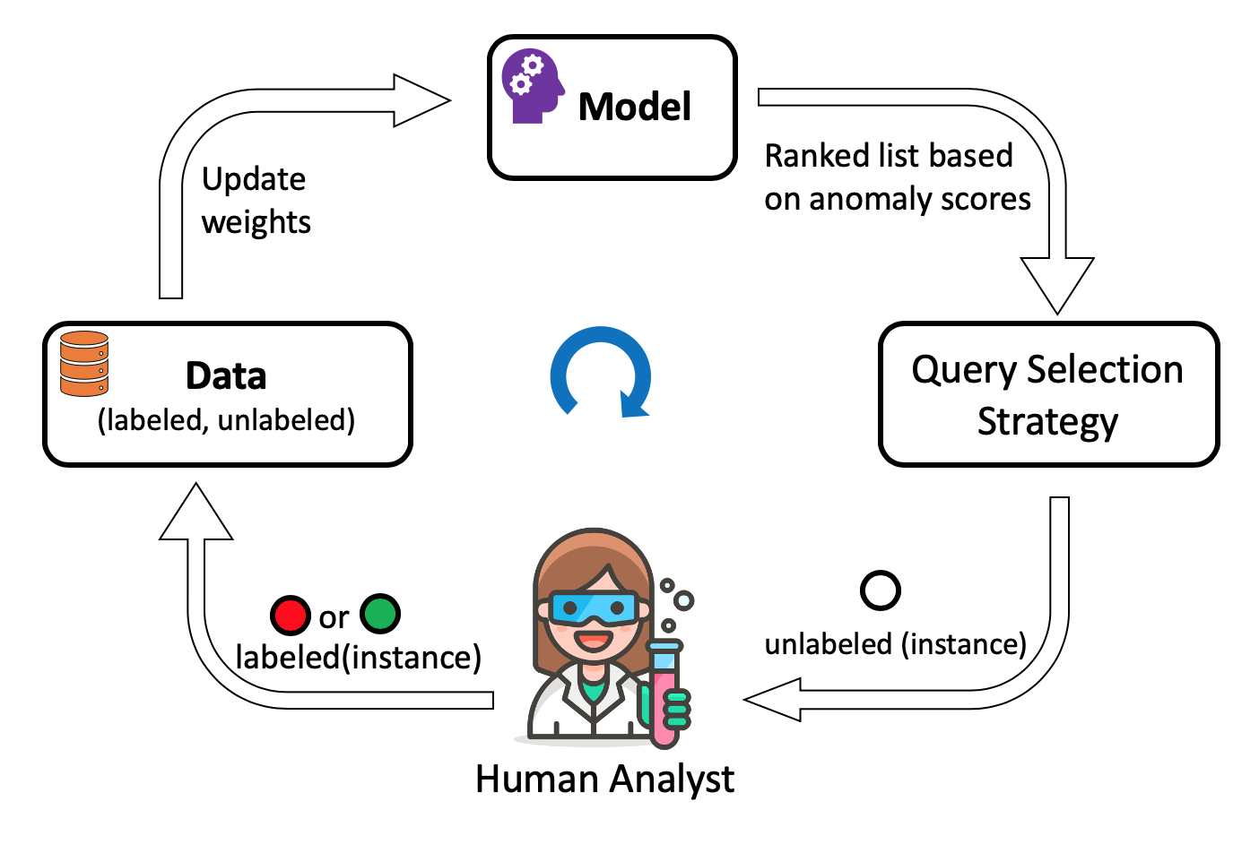
Figure 1: High-level overview of the human-in-the-loop anomaly detection framework. Our GLAD algorithm instantiates the “Model” component by placing a uniform prior over the input feature space using a neural network.

4 GLAD Algorithm

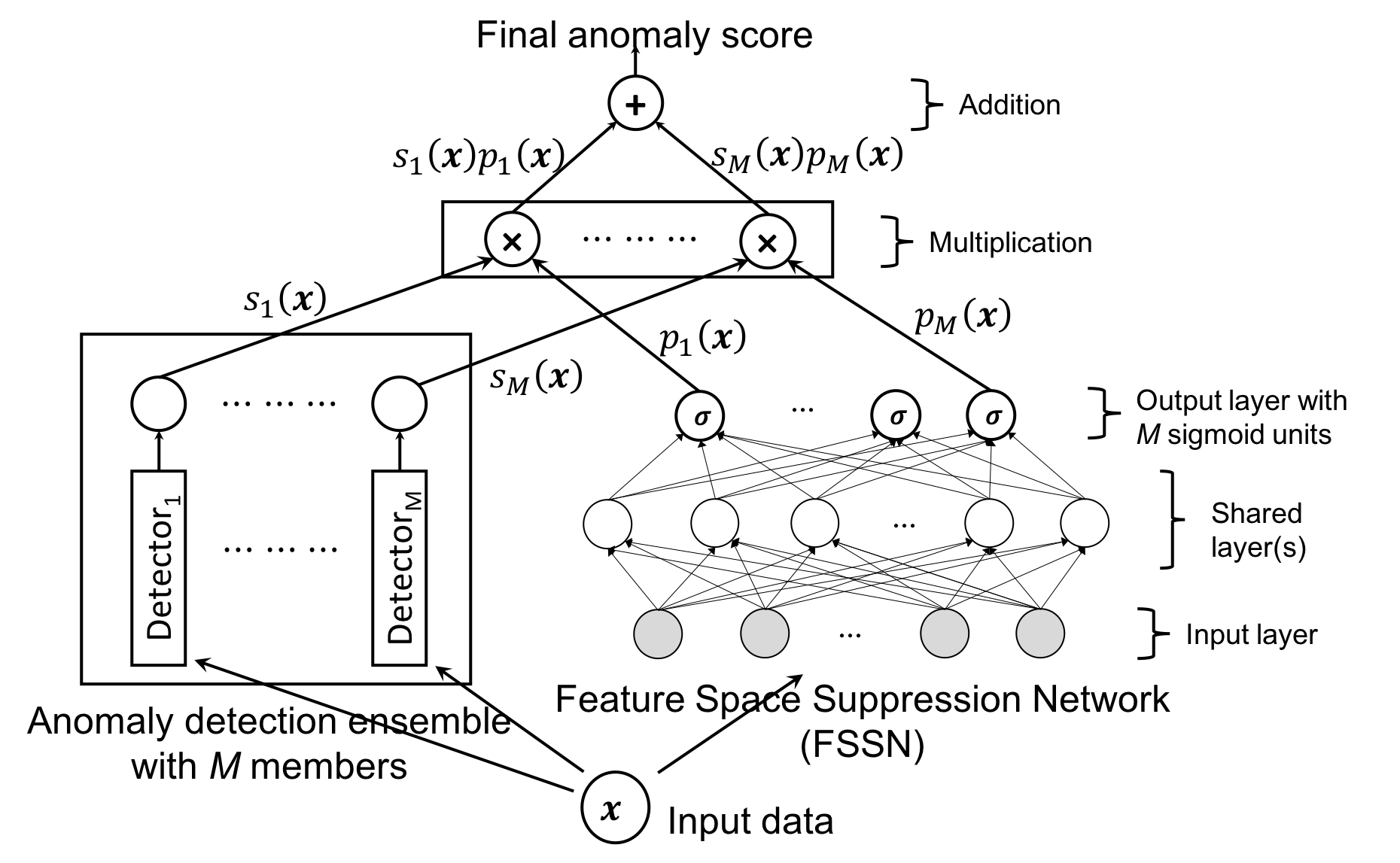
Figure 2: Overview of the model component of GLAD algorithm. The anomaly detection ensemble contains $M$ global detectors. We assume that all ensemble members are pre-trained and cannot be modified. The final layer of the Feature Space Suppression Network (FSSN) contains $M$ sigmoid outputs, each one paired with a corresponding ensemble member. Each output node in the FSSN is initially primed to predict the same probability ($0.5$ in our experiments) across the entire input feature space. FSSN learns which parts of the feature space are relevant for each detector based on the label feedback received from human analyst. For a given data instance ${\bf x}$, $s_{m}({\bf x})$ denotes the score assigned to it by the $m^{th}$ detector and $p_{m}({\bf x})$ denotes the probability computed by the FSSN that the $m^{th}$ detector is relevant. The final anomaly score for data instance ${\bf x}$ is the sum of all scores from each detector weighted by their corresponding relevance. In each iteration of the active learning loop, we select one unlabeled instance for querying, and update the weights of FSSN to adjust the local relevance of each ensemble member over all labeled instances.

Overview.

We start with the assumption that each ensemble member is uniformly relevant in every part of the input feature space. This assumption is implemented by priming a neural network referred to as FSSN (feature space suppression network) to predict the same probability value $b\in(0,1)$ for every instance in ${\bf D}$. In effect, this mechanism places a uniform prior over the input feature space $\mathcal{X}$ for the relevance of each detector. Subsequently, the algorithm receives label feedback from a human analyst and determines whether the ensemble made an error (i.e., anomalous instances are ranked at the top and scores of anomalies are higher than scores of nominals). If there is an error, the weights of FSSN are updated to suppress all erroneous detectors for similar inputs in the future. Figure 2 illustrates different components of the GLAD model including the ensemble of anomaly detectors and the Feature Space Suppression Network (FSSN). And algorithm  1 illustrates how the GLAD model fits inside the overall human-in-the loop framework. The GLAD components are highlighted inside the framework.

AAD Loss.

We employ the AAD hinge loss from (Das et al., 2018) to measure the degree of error in anomaly detection based on all labeled instances. This loss is a simplified version of the constraint-based loss proposed in (Das et al., 2016), and is more suitable for gradient-based learning. AAD makes two assumptions: (a) $\tau$ fraction of instances (a very small number of instances from ${\bf D}$) are anomalous, and (b) labeled anomalies should have scores higher than the instance currently ranked at the $\tau$-th quantile, whereas nominals should have scores lower than that instance. We will denote this loss by $\ell_{AAD}({\bf x})$.

Algorithm 1 GLAD ($B$, $\mathcal{E}$, FSSN, ${\mathbf{D}}$, ${\mathbf{H}}_{f}$, $b$)

  Input: Query budget $B$, Ensemble of global anomaly detectors $\mathcal{E}$, FSSN neural network with parameters ${\bf\Theta}$, complete dataset ${\mathbf{D}}$, labeled instances ${\mathbf{H}}_{f}\subseteq{\bf D}$, bias probability $b$

  Priming Step: Initialize FSSN to predict $b$ for all ${\bf x}\in{\bf D}$

  for $t\in\{1\cdots B\}$ do

     

     // Greedy selection: highest-scoring instance

     Let ${\bf q}={\mathbf{x}}_{i}$, where $i=\operatorname*{arg\,max}_{i}(a_{i})$

     // Aggregate set of labeled instances

     Set ${\mathbf{H}}_{f}=\{({\bf x}_{i},y_{i})\}\cup{\mathbf{H}}_{f}$

     

     

  end for

  return FSSN, ${\mathbf{H}}_{f}$

$$\ell_{prior}({\bf x})=\sum_{m=1}^{M}{-b\log(p_{m}({\bf x}))-(1-b)\log(1-p_{m}({\bf x}))}$$ (1)

$$\ell_{A}(q;({\bf x},y))=\max(0,y(q-\text{{Score}$({\bf x})$}))$$ (2)

$$\ell_{AAD}({\bf x},y)=\ell_{A}(q_{\tau}^{(t-1)};({\bf x},y))+\ell_{A}(\text{{Score}}({\bf x}_{\tau}^{(t-1)});({\bf x},y))$$ (3)

$$\ell_{FSSN}=\frac{1}{|{\bf H}_{f}^{(t)}|}\sum_{({\bf x},y)\in{\bf H}_{f}^{(t)}}\ell_{AAD}({\bf x},y)+\frac{\lambda}{|{\bf D}|}\sum_{{\bf x}\in{\bf D}}\ell_{prior}({\bf x})$$ (4)

Feature Space Suppression Network (FSSN).

The FSSN is a neural network with $M$ sigmoid activation nodes in its output layer, where each output node is paired with an ensemble member. It takes as input an instance from the original feature space and outputs the relevance of each detector for that instance. We denote the relevance of the $m^{th}$ detector to instance ${\bf x}$ by $p_{m}({\bf x})$. The FSSN is primed using the cross-entropy loss in Equation 1 such that it outputs the same probability $b\in(0,1)$ at all the output nodes for each data instance in ${\bf D}$. This loss acts as a prior on the relevance of detectors in ensemble. When all detectors have the same relevance, the final anomaly score simply corresponds to the average score across all detectors (up to a multiplicative constant), and is a good starting point for active learning.

After FSSN is primed, it automatically learns the relevance of the detectors based on label feedback from human analyst using the combined loss $\ell_{FSSN}$ in Equation 4, where $\lambda$ is the trade-off parameter. We set the value of $\lambda$ to 1 in all our experiments. $\mathbf{H}_{f}^{(t)}\subseteq{\bf D}$ in Equation 4 denotes the total set of instances labeled by the analyst after $t$ feedback iterations. ${\mathbf{x}}_{\tau}^{(t-1)}$ and $q_{\tau}^{(t-1)}$ denote the instance ranked at the $\tau$-th quantile and its score after the $(t-1)$-th feedback iteration. $\ell_{A}$ encourages the scores of anomalies in $\mathbf{H}_{f}$ to be higher than that of $q$, and the scores of nominals in $\mathbf{H}_{f}$ to be lower.

5 Explanations for Anomalies with GLAD

To help the analyst understand the results of active anomaly detection system, we now introduce the concept of “explanations” in the context of GLAD model.

• Explanation: An explanation outputs a reason why a specific data instance was assigned a high anomaly score. Generally, we limit the scope of an explanation to one data instance. The main application is to diagnose the model: whether the anomaly detector(s) are working as expected or not.

GLAD assumes that the anomaly detectors in the ensemble can be arbitrary (homogeneous or heterogeneous). The best it can offer as an explanation is to output the member which is most relevant for a test data instance. With this in mind, we can employ the following approach to generate explanations:

1. Employ the FSSN network to predict the relevance of individual ensemble members on the complete dataset. It is important to note that the relevance of a detector is different from the anomaly score(s) it assigns. A detector which is relevant in a particular subspace predicts the labels of instances in that subspace correctly irrespective of whether those instances are anomalies or nominals.

2. Find the instances for each ensemble member for which that detector is the most relevant. Mark these instances as positive and the rest as negative.

3. Train a separate decision tree for each member to separate the corresponding positives and negatives. This describes the subspaces where each ensemble member is relevant. Figure 3 illustrates this idea on the Toy dataset.

4. When asked to explain the anomaly score for a given test instance:

   1. Use FSSN network to identify the most relevant ensemble member for the test instance.

   2. Employ a model agnostic explanation technique such as LIME (Ribeiro et al., 2016) or ANCHOR (Ribeiro et al., 2018) to generate the explanation using the most relevant ensemble member. As a simple illustration, we trained GLAD on the synthetic dataset and a LODA ensemble with four projections. After $30$ feedback iterations, the unlabeled instance at $(6.12,3.04)$ had the highest anomaly score. We used LIME to explain its anomaly score. LIME explanation is shown below:

      ¯¯(’2.16 < y <= 3.31’, -0.4253)
      ¯¯(’x > 2.65’, 0.3406)
      ¯¯
      

      Here the explanation 2.16 < y <= 3.31 from member $2$ has the highest absolute weight and hence, explains most of the anomaly score.

Since most aspects of explanations are qualitative, we leave their evaluation on real-world data to future work.

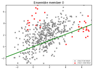
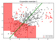
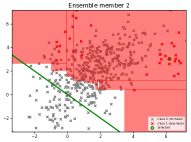
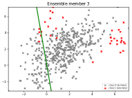
Figure 3: Most relevant ensemble members in subspaces inferred with GLAD after 30 feedback iterations. There are four members (i.e., LODA projections) in our current example. Note that members 1 and 2 were found relevant in subspaces which have mostly nominal instances. This is because they correctly assigned low anomaly scores to instances in those subspaces. The last member (member 3) did not rank as the top-most relevant detector for any instance; hence, it does not have any region marked in red. The point circled in green (in bottom left plot) is a test instance. Ensemble member 2 was found to be the most relevant for this instance.

6 Experiments and Results

In this section, we describe our experimental setup and present results on both synthetic and real-world datasets.

LODA based Anomaly Detector.

For our anomaly detector, we employ the LODA algorithm (Pevny, 2015), which is an ensemble ${\bf\mathcal{E}}=\{\mathcal{D}_{m}\}_{m=1}^{M}$ of $M$ one-dimensional histogram density estimators computed from sparse random projections. Each projection $\mathcal{D}_{m}$ is defined by a sparse $d$-dimensional random vector $\bf{\beta}_{m}$. LODA projects each data point onto the real line according to $\bf{\beta}_{m}^{\top}{\bf x}$ and then forms a histogram density estimator $f_{m}$. The anomaly score assigned to a given instance ${\bf x}$ is the mean negative log density: Score(${\bf x}$) = $\frac{1}{M}\sum_{m=1}^{M}{s_{m}({\bf x})}$, where, $s_{m}({\bf x})\triangleq-\log(f_{m}({\bf x}))$.

LODA gives equal weights to all projections. Since the projections are selected at random, there is no guarantee that every projection is good at isolating anomalies uniformly across the entire input feature space. LODA-AAD (Das et al., 2016) was proposed to integrate label feedback from a human analyst by learning a better weight vector ${\bf w}$ that assigns weights proportional to the usefulness of the projections. In this case, the learned weights are global, i.e., they are fixed across the entire input feature space. In contrast, we employ GLAD to learn the local relevance of each detector in the input space using the label feedback.

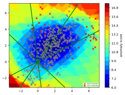
Figure 4: Baseline LODA score contours on toy dataset. Here we presented LODA with four projections (green lines) applied to the same dataset. Red represents locations with higher anomaly score and blue for nominals.

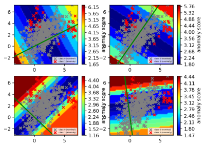
Figure 5: Score contours for each LODA projection. More red zones are possible places where anomalous candidates could be present. And dark blue zones are representing less possible places for anomalous data. For illustration purpose we are presenting 4 different projection.

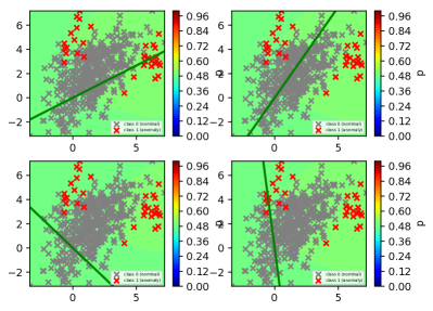
Figure 6: The red ‘$\times$’ are true anomalies and grey ‘$\times$’ are true nominals. The output nodes of the FSSN are initially primed to return a relevance of $0.5$ everywhere in the feature space.

FSSN Details.

We introduced a shallow neural network with $\max(50,3M)$ hidden nodes for all our test datasets, where $M$ is the number of ensemble members (i.e., LODA projections). The network is retrained after receiving each label feedback. This retraining cycles over the entire dataset (labeled and unlabeled) once. Since the labeled instances are very few, we up-sample the labeled data five times. We also employ $L_{2}$-regularization for training the weights of the neural network.

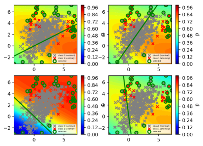
(a) Relevance after 30 feedback iterations

Figure 7: The points circled in green were shown to the analyst for labeling, one per feedback iteration. After $30$ feedback iterations, the bottom left projection was found to be most relevant in the top-right half-space, whereas it is completely irrelevant in the bottom-left half-space. Other projections were less relevant in most parts of the feature space.

Dataset	Total	Dims	# Anomalies(%)
Abalone	1920	9	29 (1.5%)
ANN-Thyroid-1v3	3251	21	73 (2.25%)
Cardiotocography	1700	22	45 (2.65%)
KDD-Cup-99	63009	91	2416 (3.83%)
Mammography	11183	6	260 (2.32%)
Yeast	1191	8	55 (4.6%)

Table 1: Description of benchmark datasets.

Synthetic Experiments.

The Toy dataset and the corresponding LODA ensembles have been shown in Figure 4. Figure 5 illustrates the aspect that detectors are varying in quality. Figure 7(a) shows that GLAD learns useful relevance information that can be of help to the analyst.

Real-world Experiments.

We demonstrate the effectiveness of GLAD on most of the datasets from Table 1 used in (Das et al., 2018). Since GLAD is most relevant when the anomaly detectors are specialized and fewer in number, we employ a LODA ensemble with maximum $15$ projections. In Figure 8, we observe that GLAD outperforms both the baseline LODA as well as LODA-AAD which weights the ensemble members globally.

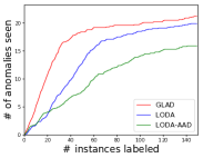
(a) Abalone

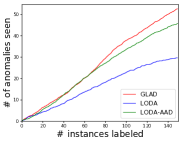
(b) ANN-Thyroid-1v3

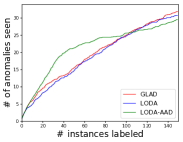
(c) Cardiotocography

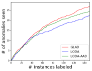
(d) Yeast

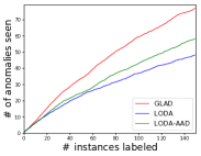
(e) Mammography

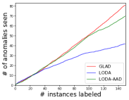
(f) KDD-Cup-99

Figure 8: Results on real-world datasets. Number of anomalies discovered as a function of the number of labeled queries. Results were averaged over $10$ different runs. The higher the curve the better the performance.

7 Discussion

It is well-known that there exists no universally applicable anomaly detector. However, sometimes a few easy-to-understand detectors meet most needs of users. Therefore, they should not be marginalized just because they fail in some special cases. Our proposed approach GLAD learns when the detectors are relevant. Therefore makes it more likely that the preferred detectors of users will be applied or suppressed as needed. Finally, it can provide explanations for the end user to acquire better understanding about the anomalies.

8 Acknowledgements

This work was supported in part by contract W911NF15-1-0461 with the US Defense Advanced Research Projects Agency (DARPA) Communicating with Computers Program and the Army Research Office (ARO), and the National Science Foundation (NSF) grant IIS-1543656 . The views expressed are those of the authors and do not reflect the official policy or position of the Department of Defense or NSF or the U.S. Government.

References

- Abe et al. (2006) Abe, N., Zadrozny, B., and Langford, J. Outlier detection by active learning. In Proceedings of the Twelth ACM SIGKDD International Conference on Knowledge Discovery and Data Mining (KDD), pp. 504–509, 2006.
- Aggarwal & Sathe (2017) Aggarwal, C. C. and Sathe, S. Outlier Ensembles. Springer, 2017.
- Almgren & Jonsson (2004) Almgren, M. and Jonsson, E. Using active learning in intrusion detection. In 17th IEEE Computer Security Foundations Workshop, (CSFW), pp. 88, 2004.
- Blanchard et al. (2010) Blanchard, G., Lee, G., and Scott, C. Semi-supervised novelty detection. Journal of Machine Learning Research, 11(Nov):2973–3009, 2010.
- Breunig et al. (2000) Breunig, M. M., Kriegel, H.-P., Ng, R. T., and Sander, J. Lof: Identifying density-based local outliers. In ACM SIGMOD International Conference on Management of Data, 2000.
- Chapelle et al. (2009) Chapelle, O., Scholkopf, B., and Zien, A. Semi-supervised learning (chapelle, o. et al., eds.; 2006)[book reviews]. IEEE Transactions on Neural Networks, 20(3):542–542, 2009.
- Das et al. (2016) Das, S., Wong, W.-K., Dietterich, T. G., Fern, A., and Emmott, A. Incorporating expert feedback into active anomaly discovery. In IEEE ICDM, 2016.
- Das et al. (2017) Das, S., Wong, W.-K., Fern, A., Dietterich, T. G., and Siddiqui, M. A. Incorporating expert feedback into tree-based anomaly detection. In KDD IDEA Workshop, 2017.
- Das et al. (2018) Das, S., Islam, M. R., Jayakodi, N. K., and Doppa, J. R. Active anomaly detection via ensembles. arXiv:1809.06477, 2018. [Online; accessed 19-Sep-2018].
- Das et al. (2020) Das, S., Wong, W.-K., Dietterich, T., Fern, A., and Emmott, A. Discovering anomalies by incorporating feedback from an expert. ACM Trans. Knowl. Discov. Data, 14(4), June 2020. ISSN 1556-4681. doi: 10.1145/3396608. URL https://doi.org/10.1145/3396608.
- Doshi-Velez & Kim (2017) Doshi-Velez, F. and Kim, B. Towards a rigorous science of interpretable machine learning. arXiv:1702.08608, 2017.
- Emmott et al. (2015) Emmott, A., Das, S., Dietterich, T. G., Fern, A., and Wong, W. Systematic construction of anomaly detection benchmarks from real data. CoRR, abs/1503.01158, 2015. URL http://arxiv.org/abs/1503.01158.
- Fürnkranz et al. (2012) Fürnkranz, J., Gamberger, D., and Lavrac, N. Foundations of Rule Learning. Cognitive Technologies. Springer, 2012.
- Goh & Rudin (2014) Goh, S. T. and Rudin, C. Box drawings for learning with imbalanced data. In The 20th ACM SIGKDD International Conference on Knowledge Discovery and Data Mining, (KDD), pp. 333–342, 2014.
- Görnitz et al. (2013) Görnitz, N., Kloft, M., Rieck, K., and Brefeld, U. Toward supervised anomaly detection. J. Artif. Intell. Res., 46:235–262, 2013.
- Guha et al. (2016) Guha, S., Mishra, N., Roy, G., and Schrijvers, O. Robust random cut forest based anomaly detection on streams. In ICML, 2016.
- He & Carbonell (2008) He, J. and Carbonell, J. G. Nearest-neighbor-based active learning for rare category detection. In NIPS, 2008.
- Jimenez (1998) Jimenez, D. Dynamically weighted ensemble neural networks for classification. In In Proceedings of the 1998 International Joint Conference on Neural Networks, pp. 753–756, 1998.
- Letham et al. (2015) Letham, B., Rudin, C., McCormick, T. H., and Madigan, D. Interpretable classifiers using rules and bayesian analysis: Building a better stroke prediction model, 2015. URL http://arxiv.org/abs/1511.01644.
- Liu et al. (2008) Liu, F. T., Ting, K. M., and Zhou, Z.-H. Isolation forest. In IEEE ICDM, 2008.
- Macha & Akoglu (2018) Macha, M. and Akoglu, L. Explaining anomalies in groups with characterizing subspace rules. Data Mining and Knowledge Discovery, 32(5):1444–1480, 2018.
- Muñoz-Marí et al. (2010) Muñoz-Marí, J., Bovolo, F., Gómez-Chova, L., Bruzzone, L., and Camp-Valls, G. Semisupervised one-class support vector machines for classification of remote sensing data. IEEE transactions on geoscience and remote sensing, 48(8):3188–3197, 2010.
- Nissim et al. (2014) Nissim, N., Cohen, A., Moskovitch, R., Shabtai, A., Edry, M., Bar-Ad, O., and Elovici, Y. Alpd: Active learning framework for enhancing the detection of malicious pdf files. In IEEE Joint Intelligence and Security Informatics Conference, 2014.
- Pevny (2015) Pevny, T. Loda: Lightweight on-line detector of anomalies. Machine Learning, 102(2):275–304, 2015.
- Ribeiro et al. (2016) Ribeiro, M. T., Singh, S., and Guestrin, C. “why should I trust you?”: Explaining the predictions of any classifier. In Proceedings of the 22nd ACM SIGKDD International Conference on Knowledge Discovery and Data Mining (KDD), pp. 1135–1144, 2016.
- Ribeiro et al. (2018) Ribeiro, M. T., Singh, S., and Guestrin, C. Anchors: High-precision model-agnostic explanations. In Proceedings of the Thirty-Second AAAI Conference on Artificial Intelligence (AAAI-18), pp. 1527–1535, 2018.
- Schölkopf et al. (2001) Schölkopf, B., Platt, J. C., Shawe-Taylor, J., Smola, A. J., and Williamson, R. C. Estimating the support of a high-dimensional distribution. Neural computation, 13(7):1443–1471, 2001.
- Senator et al. (2013) Senator, T. E., Goldberg, H. G., Memory, A., Young, W. T., Rees, B., Pierce, R., Huang, D., Reardon, M., Bader, D. A., Chow, E., Essa, I., Jones, J., Bettadapura, V., Chau, D. H., Green, O., Kaya, O., Zakrzewska, A., Briscoe, E., Mappus, R. I. L., McColl, R., Weiss, L., Dietterich, T. G., Fern, A., Wong, W.-K., Das, S., Emmott, A., Irvine, J., Lee, J.-Y., Koutra, D., Faloutsos, C., Corkill, D., Friedland, L., Gentzel, A., and Jensen, D. Detecting insider threats in a real corporate database of computer usage activity. In KDD, 2013.
- Siddiqui et al. (2018) Siddiqui, M. A., Fern, A., Dietterich, T. G., Wright, R., Theriault, A., and Archer, D. W. Feedback-guided anomaly discovery via online optimization. In Proceedings of the 24th ACM SIGKDD International Conference on Knowledge Discovery & Data Mining, (KDD), pp. 2200–2209, 2018.
- Stokes et al. (2008) Stokes, J. W., Platt, J. C., Kravis, J., and Shilman, M. Aladin: Active learning of anomalies to detect intrusions. Technique Report. Microsoft Network Security Redmond, WA, 98052, 2008.
- Veeramachaneni et al. (2016) Veeramachaneni, K., Arnaldo, I., Cuesta-Infante, A., Korrapati, V., Bassias, C., and Li, K. Ai2: Training a big data machine to defend. IEEE International Conference on Big Data Security, 2016.
- Zhu (2005) Zhu, X. J. Semi-supervised learning literature survey. Technical report, University of Wisconsin-Madison Department of Computer Sciences, 2005.