Cosmological Fluids with Logarithmic Equation of State

Abstract

We investigate the cosmological applications of fluids having an equation of state which is the analog to the one related to the isotropic deformation of crystalline solids, that is containing logarithmic terms of the energy density, allowing additionally for a bulk viscosity. We consider two classes of scenarios and we show that they are both capable of triggering the transition from deceleration to acceleration at late times. Furthermore, we confront the scenarios with data from Supernovae type Ia (SN Ia) and Hubble function observations, showing that the agreement is excellent. Moreover, we perform a dynamical system analysis and we show that there exist asymptotic accelerating attractors, arisen from the logarithmic terms as well as from the viscosity, which in most cases correspond to a phantom late-time evolution. Finally, for some parameter regions we obtain a nearly de Sitter late-time attractor, which is a significant capability of the scenario since the dark energy, although dynamical, stabilizes at the cosmological constant value.

I Introduction

One of the main aims of modern cosmology is to explain the current accelerated expansion of the Universe Riess:1998cb ; Perlmutter:1998np . According to cosmological observations at present, approximately 70% of the energy density of the Universe is attributed to a component dubbed dark energy Copeland:2006wr ; Cai:2009zp . The remaining 26% is attributed to cold dark matter (CDM) and only 4% corresponds to ordinary baryonic matter. Dark matter is necessary in order to provide an explanation to the peculiar velocities in galaxies as well as to the cluster collisions. Although dark matter may be some sort of non-interacting particle Oikonomou:2006mh , nowadays there exist various alternative proposals mimicking it Dutta:2017fjw ; Sebastiani:2016ras ; Nashed:2018aai .

In $\Lambda$CDM paradigm dark matter is modeled as a pressureless fluid, while dark energy is assumed to not interact with ordinary matter and it can be interpreted as the vacuum energy, namely a simple cosmological constant. On the other hand, in general dark energy models the accelerating expansion can be described in terms of an exotic perfect fluid with negative pressure, which satisfies a barotropic equation of state Peebles:2002gy ; Sahni:1999gb ; Li:2011sd . Hence, many studies in the literature use perfect fluids to describe various evolutionary aspects of the Universe Barrow:1994nx ; Tsagas:1998jm ; HipolitoRicaldi:2009je ; Gorini:2005nw ; Kremer:2003vs ; Carturan:2002si ; Brevik:2017juz ; Buchert:2001sa ; Hwang:2001fb ; Elizalde:2009gx ; Cruz:2011zza ; Oikonomou:2017mlk ; Brevik:2017msy ; Capozziello:2006dj ; Elizalde:2017dmu ; Brevik:2016kuy ; Balakin:2012ee ; Brevik:2018azs , while the most general models of dark fluids can be incorporated using an inhomogeneous equation of state Nojiri:2005sr ; Nojiri:2006zh ; Elizalde:2005ju . Finally, an alternative description of the dark energy sector can arise effectively through gravitational modifications reviews1 ; reviews2 ; reviews3 ; reviews4 ; reviews4b ; reviews5 ; reviews6 ; reviews7 .

As it is known, the standard cold dark matter scenario provides very efficient results at large (cosmological) scales, but it might be problematic at galactic scales. These problems may be connected to the assumption that dark matter is pressureless. Nevertheless, the description of the late-time Universe at small scales can be achieved through the framework of the logarithmic-corrected equation of state for the matter sector, within the Debye approximation Intermetallics1 ; Intermetallics2 . In this formulation the fluid pressure is modeled by an empirical formula for the pressure of the deformed crystalline solids under the isotropic stress Ivanovskii . In order for the Universe to change under the action of cosmic expansion, it is necessary that the fluid pressure, described in terms of an equation of state, to be negative reviews1 ; reviews2 ; reviews3 . The negative pressure in the logarithmic-corrected equation of state scenarios becomes dominant when the volume of the Universe exceeds a certain value. This scenario corresponds to the approaches of logotropic dark energy model (LDE) Chavanis:2014hba ; Chavanis:2015eka .

In the present work we are interested in studying the dynamical evolution of a late-time Universe by assuming a modified log-corrected power-law equation of state (EoS) for the dark energy fluid, allowing additionally the fluid to be viscous. In particular, we examine in detail various forms of the dark energy EoS and we investigate how the Universe evolution is affected by the corresponding EoS. Moreover, we shall assume that a non-trivial interaction between the dark energy and dark matter fluids may exist, and by conveniently choosing the EoS we shall investigate the dynamical behavior of the cosmological system in terms of an autonomous dynamical system. The motivation for using non-trivial interaction between the dark sectors arises mainly from the fact that dark energy dominates over dark matter at late times, and thus it is possible that the dark matter sector loses its energy feeding the dark energy sector and providing an alleviation to the coincidence problem Gondolo:2002fh ; Farrar:2003uw ; Cai:2004dk ; Wang:2006qw ; Bertolami:2007zm ; Chen:2008ft ; He:2008tn ; Valiviita:2008iv ; Jackson:2009mz ; Jamil:2009eb ; He:2010im ; Boehmer:2008av ; Bamba:2012cp ; Bolotin:2013jpa ; Costa:2013sva ; Nunes:2016dlj ; Odintsov:2018awm ; Odintsov:2018uaw . The resulting picture of the coupled dark energy - dark matter system is quite interesting as we demonstrate, since for a class of parameter values the dynamical system has a stable asymptotic attractor, which corresponds to an accelerating phantom fixed point. Notably, this phantom attractor can become a nearly de Sitter attractor if the model parameters are chosen appropriately.

This paper is organized as follows: In section II we present in brief the motivation and the structure of the proposed EoS. In section III we discuss the cosmological applications of two scenarios, with emphasis given in the late-time era. In section IV we briefly discuss the observational constraints and implications of the logarithmic corrected EoS dark energy fluid. In section V we apply the dynamical system method in order to investigate the coupled dark energy-dark matter system, with the dark energy sector being described by a viscous logarithmic EoS of a specific form. Finally, the conclusions follow at the end of the paper.

II Viscous logarithmic-corrected power-law fluid

Our purpose is to study dark energy in terms of a logarithmic-corrected power-law fluid. The EoS of such a fluid has the form Capozziello:2017buj

$$p=A\left(\frac{\rho}{\rho^{*}}\right)^{-l}\ln\left(\frac{\rho}{\rho^{*}}\right),$$ (1)

where $\rho^{*}$ is a reference density, which is identified with the Planck density in Chavanis:2014hba , namely $\rho_{Pl}=c^{5}/(\hbar G)\approx 5.16\times 10^{99}gr/m^{3}$. In the new notation $A>0$ represents the logotropic temperature, while $l=-\frac{1}{6}-\gamma_{G}$, with $\gamma_{G}$ the dimensional Gruneisen parameter. For $l=0$ we obtain the equation of state for the logotropic cosmological model Chavanis:2014hba . It is interesting that the EoS of Eq. (1) may have deep relation with equations of state found in condensed matter fluids, introduced in Refs. Intermetallics1 ; Intermetallics2 .

Let us rewrite (1) in the notation of a logotropic dark energy model LDE model. For this purpose we express the volume in terms of mass density, using the relation Chavanis:2014hba ; Chavanis:2015eka

$$p(V)=-\beta\left(\frac{V}{V_{0}}\right)^{-\frac{1}{6}-\gamma_{G}}\ln\left(\frac{V}{V_{0}}\right),$$ (2)

where $V_{0}$ is a volume, which presents a barrier among the different signs of the pressure $p$, and $\beta$ is a bulk modulus at $V_{0}$. The bulk modulus shows how much the volume changes under the action of external forces. The parameter $\gamma_{G}$ in the homogeneous and isotropic Universe is a free parameter of the theory. When $V<V_{0}$ the pressure is positive for the positive bulk modulus, and it is negative in the case of an inequality of the opposite sign. If the pressure of the dark fluid satisfies relation (2), then in order to ensure the cosmic acceleration the volume must overcome the barrier $V\approx V_{0}$. There are three different regimes of the behavior of the pressure (2) Capozziello:2017buj :

1. The era before passing the $V_{0}$ barrier, when $V<V_{0}$. Then the pressure is positive and the Universe is decelerating. This case corresponds to the case of the pressureless matter in the $\Lambda$CDM model.

2. The era of equivalence between volumes, when $V=V_{0}$. That is the transition time from the deceleration to the acceleration era.

3. The era after passing the $V_{0}$ barrier, when $V>V_{0}$. Then the pressure is negative and the fluid starts to trigger the Universe acceleration. Thus, in the logarithmic-corrected power-law model, the dynamical evolution of the Universe is described by a single fluid, which accelerates the Universe, when its volume passes the barrier $V=V_{0}$. This allows us to apply this model to the description of the late Universe.

We consider a homogeneous and isotropic on large scales flat geometry, and we desire to study the dynamical evolution of the Universe using a fluid described by the logarithmic EoS (1). For generality, we additionally allow for viscosity of the fluid. In order to achieve this we modify equation (1) adding the term which describes viscosity, namely

$$\zeta(H,t)=\xi_{1}(t)(3H)^{n},$$ (3)

where $\zeta(H,t)$ is the bulk viscosity which depends on the Hubble parameter $H$ and on the time $t$. From thermodynamic considerations it follows that $\zeta(H,t)>0$.

In summary, in view of the above considerations, the EoS for the logarithmic-corrected power-law fluid has the form

$$p=A\left(\frac{\rho}{\rho^{*}}\right)^{-l}\ln\left(\frac{\rho}{\rho^{*}}\right)-3H\zeta(H,t).$$ (4)

In the next section we shall investigate the evolution of the Universe for various forms of the dark energy EoS.

III Cosmology with viscous logarithmic-corrected power-law fluid

In this section we will study the late-time behavior of the Universe by using an inhomogeneous viscous fluid description of dark energy. We consider a spatially flat Friedmann-Robertson-Walker (FRW) space-time with line element

$$ds^{2}=-dt^{2}+a(t)^{2}\delta_{ij}dx^{i}dx^{j}\,,$$ (5)

where $a(t)$ is the scale factor.

The logarithmic-corrected power-law fluid model cannot describe the early Universe, because the temperature during this era is much greater than the Debye temperature of solids. The fluid in the inflationary epoch becomes pressureless as in the case of LDE model Chavanis:2016pcp , while at late times the pressure tends to a constant negative value and thus it provides the necessary requirement for triggering the acceleration. Additionally, the incorporation of viscosity improves the singularity structure of the cosmological system at hand, and the behavior of the Universe in the vicinity of a Big Rip Caldwell:1999ew ; Caldwell:2003vq ; Faraoni:2001tq ; Nojiri:2003vn or of types II, III and IV singularities Barrow:2004xh ; Nojiri:2004ip , the classification of which was first given in Nojiri:2005sx .

Let us first consider the non-interacting scenario, in which case $\rho$ fulfills the standard conservation equation

$$\dot{\rho}+3H(\rho+p)=0\,,$$ (6)

where $H=\dot{a}/a$ is the Hubble function, and $p$ is given by (4). In the following two subsections we study two scenarios with different fluid viscosity form.

III.1 Viscosity with constant function $\xi_{1}(t)$

We start by considering the bulk viscosity in the expression (3) to have the following simple form:

$$\zeta(H,t)=3\alpha H\,,$$ (7)

where $\alpha$ is a positive constant, since such a linear-in-$H$ form is widely used in viscous cosmology Brevik:2017msy . Hence, inserting (4) and (7) into (6), and using the Friedmann equation we obtain

$$\dot{\rho}+3H\Big{[}A\left(\frac{\rho}{\rho_{*}}\right)^{-l}\ln\frac{\rho}{\rho_{*}}+\theta\rho\Big{]}=0\,,$$ (8)

where $\theta=1+3\alpha\kappa^{2}$, with $\kappa^{2}=8\pi G$ and $G$ denoting the Newton’s gravitational constant.

In the low-energy regime ($\rho\ll\rho_{*}$), and for $l=-1$, equation (8) simplifies as

$$\dot{\rho}+\frac{3H}{\rho_{*}}\Big{[}A(\rho-\rho_{*})+\theta\rho\rho_{*}\Big{]}=0\,,$$ (9)

which using the second Friedmann equation becomes

$$\dot{H}+d\,H^{2}-b=0\,,$$ (10)

where $d=\frac{3}{2}(A+\theta\rho_{*})$ and $b=\frac{1}{2}A\kappa^{2}\rho_{*}$ (note that $b>0$ since $A>0$). The solution of equation (10) is found to be

$$H(t)=\sqrt{\frac{b}{d}}\frac{e^{\sqrt{bd}t}+C_{1}e^{\sqrt{bd}t}}{e^{\sqrt{bd}t}-C_{1}e^{\sqrt{bd}t}}\,,$$ (11)

where $C_{1}$ is an arbitrary constant. As we observe, the Hubble function $H(t)$ diverges for $t\to 0$ and a Big Bang type singularity occurs. Additionally, taking $C_{1}=1$ for simplicity, the scale factor is given by the expression

$$a(t)=a_{0}\sinh(\sqrt{bd}t)^{1/d}\,,$$ (12)

with $a_{0}$ an integration constant, while its second derivative reads as

$$\ddot{a}=\frac{b}{d}\left[\frac{\cosh^{2}\left(\sqrt{bd}t\right)-d}{\sinh^{2}\left(\sqrt{bd}t\right)}\right]a(t)\,.$$ (13)

Hence, we obtain $\ddot{a}=0$ at $t_{0}=\frac{1}{\sqrt{bd}}\ln\left(\sqrt{d}+\sqrt{d-1}\right)$. If $d<1$, or equivalently if $A<\frac{2}{3}-\theta\rho_{*}$, then the second derivative of the scale factor is positive and the Universe transits to an accelerated expansion. On the other hand, in the case $d>1$, then for $0<t<t_{0}$ the second derivative is negative, i.e. the expansion is decelerating, while for $t>t_{0}$ the Universes enters in an accelerating era. Therefore, we are able to obtain the transition from a decelerating to an accelerating epoch. Finally, note that from (12) we find that

$$\dot{H}(t)=-\frac{b}{\sinh^{2}\left(\sqrt{bd}t\right)}\,,$$ (14)

and thus we deduce that since $\dot{H}(t)<0$ we obtain a Universe that does not super-accelerate. Lastly, we mention here that in the case of zero viscosity (i.e. for $\alpha=0$) we obtain $\theta=1$ and thus the above analysis is significantly simplified.

In summary, the model at hand can describe the Universe evolution, with transition from deceleration to acceleration epoch. We mention that we have not considered an explicit cosmological constant, and thus the above behavior arises only due to the model dynamics.

III.2 Viscosity with a linear time-dependent function $\xi_{1}(t)$

Let us now assume that the function $\xi_{1}(t)$ in (3) has the form

$$\xi_{1}(t)=d_{1}t+b_{1},$$ (15)

with $d_{1}$ and $b_{1}$ being arbitrary parameters, that is we consider the bulk viscosity to have the following simple form:

$$\zeta(H,t)=3H(d_{1}t+b_{1})\,.$$ (16)

Thus, inserting (4) and (16) into (6), and using the Friedmann equation we acquire

$$\dot{\rho}+3H\Big{[}A\left(\frac{\rho}{\rho_{*}}\right)^{-l}-A\left(\frac{\rho}{\rho_{*}}\right)^{-l-1}+(\tilde{c}t+\tilde{b})\rho\Big{]}=0\,,$$ (17)

where $\tilde{c}=3d_{1}\kappa^{2}$ and $\tilde{b}=1-3b_{1}\kappa^{2}$. In the case $l=-1$ , using the second Friedmann equation we can rewrite (17) as

$$2\dot{H}+3\left(\tilde{c}t+\tilde{b}+\frac{A}{\rho_{*}}\right)H^{2}=0\,,$$ (18)

which has the solution

$$H(t)=\frac{4}{3\left(\tilde{c}t+\tilde{b}+\frac{A}{\rho_{*}}\right)^{2}+C_{2}}\,,$$ (19)

with $C_{2}$ an integration constant. Without loss of generality we focus on the case $C_{2}=0$. Firstly, we can see that the Hubble rate $H(t)$ diverges at the finite time $t_{0}=-\frac{1}{\tilde{c}}\left(\tilde{b}+\frac{A}{\rho_{*}}\right)$, and thus a Big Rip type singularity occurs. Concerning the scale factor, solution (19) leads to

$$a(t)=a_{0}\exp\Big{[}-\frac{4}{3\tilde{c}}\left(\tilde{c}t+\tilde{b}+\frac{A}{\rho_{*}}\right)^{-1}\Big{]}\,,$$ (20)

with $a_{0}$ an integration constant, while its second derivative is

$$\ddot{a}(t)=\Big{[}1-\frac{3}{2}\tilde{c}\left(\tilde{c}t+\tilde{b}+\frac{A}{\rho_{*}}\right)\Big{]}H^{2}(t)a(t)\,.$$ (21)

As we observe, $\ddot{a}=0$ at $t_{1}=\frac{1}{\tilde{c}}\Big{[}\frac{2}{3\tilde{c}}-\tilde{b}-\frac{A}{\rho_{*}}\Big{]}$. Thus, in the case $\tilde{c}>0$, for values $t<t_{1}$, it turns out that $\ddot{a}<0$, and therefore the Universe experiences a decelerated expansion, while for $t>t_{1}$ we have $\ddot{a}>0$ and the Universe transits to a late-time accelerated era.

In summary, the model at hand can describe the Universe’s evolution, with the transition from decelerating to accelerating epoch. We mention that this behavior is obtained although we have not considered an explicit cosmological constant.

IV Observational Constraints

As we saw, the scenario at hand can give rise to a Universe that experiences the transition from a decelerating era to an accelerating epoch. In order to perform a confrontation with observations we will use the Supernovae type Ia (SN Ia) data, as well as direct measurements of the Hubble parameter with the corresponding covariance matrix.

IV.1 Supernovae Type Ia:

In these observational data sets, the apparent luminosity $l(z)$ (or equivalently the apparent magnitude $m(z)$), is measured as a function of the redshift, and is related to the luminosity distance as

$$2.5\log\left[\frac{L}{l(z)}\right]=\mu\equiv m(z)-M=5\log\left[\frac{d_{L}(z)_{\text{obs}}}{Mpc}\right]+25,$$ (22)

where $M$ is the absolute magnitude and $L$ is the luminosity. Moreover, for any model under consideration one can calculate the theoretically predicted dimensionless luminosity distance $d_{L}(z)_{\text{th}}$ using the theoretically predicted evolution of the Hubble function through

$$d_{L}\left(z\right)_{\text{th}}\equiv\left(1+z\right)\int^{z}_{0}\frac{dz^{\prime}}{H\left(z^{\prime}\right)}\leavevmode\nobreak\ .$$ (23)

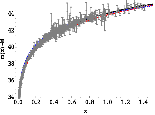
Figure 1: The theoretically predicted apparent minus absolute magnitude as a function of the redshift, for the logarithmic-corrected fluid (4) with viscosity (7) (i.e. constant function $\xi_{1}(t)$), for $a_{0}=1$ and $b=0.25\times 10^{-120}$, in units where $\kappa^{2}=c=\hbar=1$ (i.e where $H(z=0)\equiv H_{0}\approx 6\times 10^{-61}$). The red-dashed curve is for $d=1$, while the blue-dotted curve is for $d=2$. The observational points correspond to the $580$ SN Ia data points from Suzuki:2011hu , and for completeness and comparison we depict the prediction of $\Lambda$CDM cosmology with the black-solid curve.

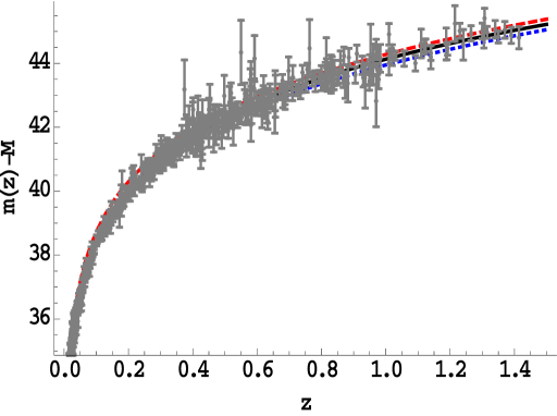
Figure 2: The theoretically predicted apparent minus absolute magnitude as a function of the redshift, for the logarithmic-corrected fluid (4) with the viscosity (16) (i.e. linear time-dependent function $\xi_{1}(t)$), for $a_{0}=5$ in units where $\kappa^{2}=c=\hbar=1$ (i.e where $H(z=0)\equiv H_{0}\approx 6\times 10^{-61}$). The red-dashed curve is for and $\tilde{c}=0.51\times 10^{-30}$, while the blue-dotted curve is for $\tilde{c}=0.55\times 10^{-30}$. The observational points correspond to the $580$ SN Ia data points from Suzuki:2011hu , and for completeness and comparison we depict the prediction of $\Lambda$CDM cosmology with the black-solid curve.

In the scenarios of the logarithmic-corrected fluid (4) of the present work, the functions $H(t)$ and $a(t)$ are known, namely relations (11),(12) for the case of viscosity (7) (i.e. constant function $\xi_{1}(t)$), and relations (19),(20) for the case of viscosity (16) (i.e. linear time-dependent function $\xi_{1}(t)$). Thus, $H(z)$ can be easily calculated since the redshift is defined as $1+z=1/a$ in the case where we set the present value of the scale factor to 1. Hence, for the case of the model with viscosity (7) we can find that

$$H(z)=\sqrt{\frac{b}{d}}\sqrt{1+[a_{0}(1+z)]^{2d}},$$ (24)

where according to the definitions below (10) the corresponding fluid parameters are

$$A=\frac{2b}{\kappa^{2}\rho_{*}}$$

$$\alpha=\frac{1}{3\kappa^{2}}\left(\frac{2d}{3\rho_{*}}-\frac{2b}{\kappa^{2}\rho_{*}^{2}}-1\right).$$ (25)

Similarly, for the case of the model with viscosity (16) we can find that

$$H(z)=\frac{3}{4}\tilde{c}^{2}\ln^{2}[a_{0}(1+z)],$$ (26)

where as we mentioned $d_{1}=\tilde{c}/(3\kappa^{2})$.

In Fig. 1 we depict the theoretically predicted apparent minus absolute magnitude as a function of $z$, for the scenario of the logarithmic-corrected fluid (4) with the viscosity (7), as well as the prediction of $\Lambda$CDM cosmology, on top of the $580$ SN Ia observational data points from Suzuki:2011hu . Similarly, in Fig. 2 we depict the same graphs, but for the case of the viscosity (16). As we can see, for both models the agreement with the SN Ia data is excellent. We mention that this behavior arises from both the logarithmic correction as well as from the viscosity terms. Interestingly enough, the scenario at hand is practically indistinguishable from $\Lambda$CDM cosmology, although we have not considered an explicit cosmological constant. This feature reveals the capabilities of the scenario.

IV.2 $H(z)$ probes

In this subsection we will use the $H(z)$ Hubble function observations in order to impose constraints on the free model parameters Farooq:2016zwm ; Capozziello:2017nbu ; Capozziello:2018jya ; Basilakos:2018arq . In particular, we will use the set given in Farooq:2016zwm , which contains $N=38$ entries in the redshift interval $0.07\leq z\leq 2.36$. As it known, the nominal chi-square function reads as Basilakos:2018arq

$$\chi^{2}_{H}(\phi^{\mu})={\mathbf{V}}{\mathbf{C}}^{-1}_{\text{c}ov}{\mathbf{V}}^{T},$$ (27)

with $\phi^{\mu}$ the statistical vector that contains the free parameters, ${\mathbf{C}}^{-1}_{\text{c}ov}$ the inverse of the covariance matrix and ${\mathbf{V}}=\{H_{D}(z_{1})-H_{M}(z_{1},\phi^{\mu}),...,H_{D}(z_{N})-H_{M}(z_{N},\phi^{\mu})\}$. Moreover, $z_{i}$ are the observed redshifts, while the letters $M$ and $D$ denote the data and models respectively. Hence, the theoretical Hubble parameter is parametrized as

$$H_{M}(z,\phi^{\mu})=H_{0}E(z,\phi^{\mu+1}),$$ (28)

and therefore

$${\mathbf{V}}=\{H_{D}(z_{1})-H_{0}E(z_{1},\phi^{\mu+1}),..,H_{D}(z_{N})-H_{0}E(z_{N},\phi^{\mu+1})\},$$ (29)

with $H_{0}$ the Hubble constant at present, $E(z)^{2}=H(z)^{2}/H_{0}^{2}$ the dimensionless Hubble function, and where the vector $\phi^{\mu+1}$ contains the model free parameters.

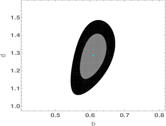
Figure 3: Contour plots for the free parameters $b$ and $d$, for $a_{0}=1$, for the model of the logarithmic-corrected fluid (4) with viscosity (7). The gray and black regions correspond respectively to 1$\sigma$ and 2$\sigma$ confidence level in the case of $H(z)$ data sets of Farooq:2016zwm , while the light blue dot marks the best-fit values.

The usual way to proceed is to introduce the standard $\chi^{2}$ estimator and impose the exact value of $H_{0}$ ($H_{0}=73.24\pm 1.74$ Km/s/Mpc) found by the SNIa team (Riess et al. Riess:2016jrr ). However, and in order to bypass the $\sim 3\!-\!3.5\ \sigma$ tension with the Planck Probe ($H_{0}=67.8\pm 0.9$ Km/s/Mpc Adam:2015rua ), we follow Basilakos:2018arq and we treat $H_{0}$ as a free parameter.

In Fig. 3 we depict the 1$\sigma$ and 2$\sigma$ likelihood contours for the free parameters $b$ and $d$, as well as the corresponding best-fit values, for the model of the logarithmic-corrected fluid (4) with viscosity (7). Similarly, in Fig. 4 we present the same graphs for the case of the viscosity (16). As we observe, both models can be in agreement with observations, which is an advantage of the scenario. Moreover, while in the first model the free parameters are significantly constrained, in the second model the agreement with the data can be obtained for a wide parameter range.

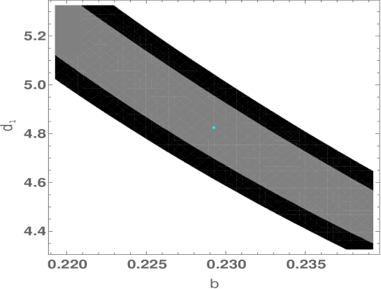
Figure 4: Contour plots for the free parameters $b_{1}$ and $d_{1}$, for free $a_{0}$, for the model of the logarithmic-corrected fluid (4) with viscosity (16). The gray and black regions correspond respectively to 1$\sigma$ and 2$\sigma$ confidence level in the case of $H(z)$ data sets of Farooq:2016zwm , while the light blue dot marks the best-fit values.

V Dynamical system analysis

In this section we apply the powerful method of dynamical system analysis in order to investigate the full system of cosmological equations. This method allows to extract information about the global behavior of a cosmological scenario, bypassing the complexity of the involved equations Leon2011 ; Bahamonde:2017ize ; Copeland:1997et ; Leon:2009rc ; Leon:2010pu ; Kofinas:2014aka ; Odintsov:2017tbc ; Oikonomou:2017ppp ; Kleidis:2018cdx . In order to be fully general, in the following we will assume an integration between the dark energy and the matter fluids, which is widely used since it can provide an alleviation to the coincidence problem while it cannot be theoretically excluded Gondolo:2002fh ; Farrar:2003uw ; Cai:2004dk ; Wang:2006qw ; Bertolami:2007zm ; Chen:2008ft ; He:2008tn ; Valiviita:2008iv ; Jackson:2009mz ; Jamil:2009eb ; He:2010im ; Boehmer:2008av ; Bamba:2012cp ; Bolotin:2013jpa ; Costa:2013sva ; Nunes:2016dlj ; Odintsov:2018awm ; Odintsov:2018uaw .

Our aim is to investigate the phase structure of a coupled dark energy system, with the dark energy sector having an EoS which has a logarithmic dependence and bulk viscosity. In this case the two Friedmann equations write as

$$H^{2}=\frac{\kappa^{2}}{3}\rho_{tot}\,,$$ (30)

$$\dot{H}=-\frac{\kappa^{2}}{3}\left(\rho_{tot}+p_{tot}\right)\,,$$ (31)

where $\rho_{tot}=\rho_{d}+\rho_{m}$ and $p_{tot}=p_{d}+p_{m}$, with $\rho_{d}$ and $\rho_{m}$ the energy densities and $p_{d}$ and $p_{m}$ the pressures of the two fluids. Concerning the matter fluid we assume it to be pressureless, namely $p_{m}=0$, while for the dark energy fluid we consider the logarithmic EoS with bulk viscosity

$$p_{d}=A\kappa^{2}\rho_{d}\ln(\kappa^{2}\rho_{d})-A\kappa^{2}\rho_{d}\ln(3H^{2})\,,$$ (32)

where $A$ is the model parameter. In the interacting scenario at hand the conservation equations for the two fluids are written as

$$\dot{\rho}_{m}+3H\rho_{m}=-Q\,$$ (33)

$$\dot{\rho}_{d}+3H(\rho_{d}+p_{d})=Q\,,$$

with $Q$ being the interaction between the dark fluids. The algebraic sign of the interaction term $Q$ determines which fluid loses energy, thus if $Q>0$ it implies that dark matter sector loses energy towards the dark energy one. We shall use a phenomenologically motivated interaction term of the form CalderaCabral:2008bx ; Pavon:2005yx ; Quartin:2008px ; Sadjadi:2006qp ; Zimdahl:2005bk ,

$$Q=3H(c_{1}\rho_{m}+c_{2}\rho_{d})\,,$$ (34)

with $c_{1}$, $c_{2}$ real constants.

Having Eqs. (30), (31) and (33) at hand we construct an autonomous dynamical system by choosing the dimensionless variables

$$x_{1}=\frac{\kappa^{2}\rho_{d}}{3H^{2}},\,\,\,x_{2}=\frac{\kappa^{2}\rho_{m}}{3H^{2}},\,\,\,z=\kappa^{2}H^{2}\,.$$ (35)

The variables of the dynamical system $x_{1}$ and $x_{2}$ satisfy the Friedmann constraint,

$$x_{1}+x_{2}=1\,,$$ (36)

which is essentially the Friedmann equation (30). Additionally, the total equation of state parameter $w_{eff}$, defined as

$$w_{eff}=\frac{p_{d}}{\rho_{tot}}\,,$$ (37)

can easily be expressed in terms of the dynamical system parameters $x_{1}$, $x_{2}$ and $z$ (35) in the following way:

$$w_{eff}=\tilde{A}x_{1}\ln x_{1}\,,$$ (38)

with

$$\tilde{A}=A\kappa^{2}\,.$$ (39)

Moreover, the interaction term $Q$ appearing in (34), expressed in terms of the variables $x_{1}$, $x_{2}$ and $z$ (35) is written as

$$\frac{\kappa^{2}Q}{3H^{3}}=3c_{1}x_{2}+3c_{2}x_{1}\,.$$ (40)

By combining Eqs. (30), (31), (33), (40) and (35), and also by using the $e$-foldings number $N$ as a dynamical variable instead of the cosmic time $t$, we obtain the following dynamical system:

$$\frac{\mathrm{d}x_{1}}{\mathrm{d}N}=3\tilde{A}(x_{1}-1)x_{1}\ln(x_{1})-(c_{1}x_{2}+c_{2}x_{1})+3x_{1}^{2}+3x_{1}(x_{2}-1)\,,$$

$$\frac{\mathrm{d}x_{2}}{\mathrm{d}N}=3\tilde{A}x_{1}x_{2}\log(x_{1})+c_{1}x_{2}+c_{2}x_{1}+3(x_{1}-1)x_{2}+3x_{2}^{2}\,,$$

$$\frac{\mathrm{d}z}{\mathrm{d}N}=-3\tilde{A}x_{1}z\log(x_{1})-3x_{1}z-3x_{2}z\,.$$ (41)

The fixed points $\phi_{*}^{1}=(x_{1},x_{2},z)$ of the above dynamical system, which are obtained by setting the left-hand-sides of the equations to zero, cannot easily be found analytically, and therefore we will investigate the phase space behavior by solving numerically the dynamical system and by using various initial conditions. Additionally, the stability of the fixed points can be investigated by calculating explicitly the Jacobian of the dynamical system at the fixed point $\phi_{*}^{1}$. The Jacobian matrix, which we denote as $\mathcal{J}$, corresponds to the linearized dynamical system near the resulting fixed point, namely

$$\mathcal{J}=\sum_{i}\sum_{j}\Big{[}\frac{\mathrm{\partial f_{i}}}{\partial x_{j}}\Big{]}\,.$$ (42)

The Jacobian matrix $\mathcal{J}$ must be evaluated exactly at the fixed points, and the corresponding eigenvalues indicate whether the particular fixed point is stable or not, whenever the fixed point is hyperbolic (the eigenvalues of the Jacobian at the fixed point have real parts which are non-zero). In the case at hand, the Jacobian matrix of the dynamical system (41) is

$$\mathcal{J}=\left(\begin{array}[]{ccc}-24x_{1}+3x_{2}+(30-60x_{1})\log(x_{1})+26&3x_{1}-1&0\\ -30\log(x_{1})x_{2}-27x_{2}+1&-30\log(x_{1})x_{1}+3x_{1}+6x_{2}-2&0\\ 3z(10\log(x_{1})+9)&-3z&30x_{1}\log(x_{1})-3(x_{1}+x_{2})\\ \end{array}\right)\,.$$ (43)

A thorough investigation of the parameter space reveals that the sign of the parameter $\tilde{A}$, and also the sign of the parameters $c_{1}$ and $c_{2}$, crucially affect the behavior of the dynamical system. Actually, for a wide range of values, the dynamical system is strongly unstable, however there are some regions of the parameter space for which stability occurs. These stability regions are the most interesting ones, from the physical point of view.

Case I: $c_{1}>0$, $c_{2}>0$, and $\tilde{A}>0$: Strong Instability of Phase Space, Variables Blow-up.
Case II: $c_{1}<0$, $c_{2}<0$, and $\tilde{A}>0$: Strong Instability of Phase Space, Variables Blow-up.
Case III: $c_{1}>0$, $c_{2}=0$, and $\tilde{A}>0$: Strong Instability of Phase Space, Variables Blow-up.
Case IV: $c_{1}=0$, $c_{2}>0$, and $\tilde{A}>0$: Strong Instability of Phase Space, Variables Blow-up.
Case V: $c_{1}=0$, $c_{2}<0$, and $\tilde{A}>0$: Strong Instability of Phase Space, Variables Blow-up.
Case VI: $c_{1}<0$, $c_{2}=0$, and $\tilde{A}>0$: Strong Instability of Phase Space, Variables Blow-up.
Case VII: $c_{1}>0$, $c_{2}=0$, and $\tilde{A}>0$: Strong Instability of Phase Space, Variables Blow-up.
Case VIII: $c_{1}<0$, $c_{2}<0$, and $\tilde{A}<0$: Strong Instability of Phase Space, Variables Blow-up.
Case IX: $c_{1}>0$, $c_{2}>0$, and $\tilde{A}<0$: Stable Fixed Point.
Case X: $c_{1}>0$, $c_{2}=0$, and $\tilde{A}<0$: Stable Fixed Point.
Case XI: $c_{1}=0$, $c_{2}>0$, and $\tilde{A}<0$: Stable Fixed Point.

Table 1: Stability regions of the phase space of the dynamical system corresponding to the two-fluids Universe (41).

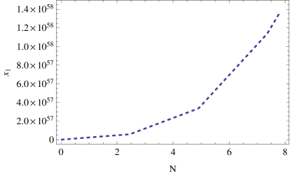
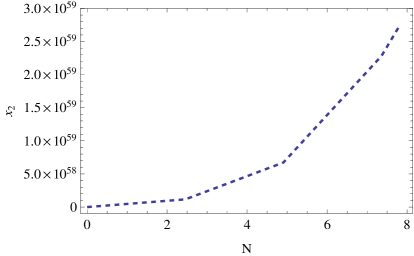
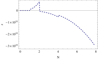
Figure 5: The evolution of the variables $x_{1}(N)$ (left), $x_{2}(N)$ (right) and $z(N)$ (bottom) as functions of the $e$-foldings number $N$, for $c_{1}=c_{2}=1$ and $\tilde{A}=10$.

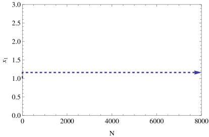
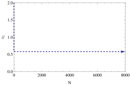
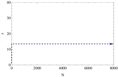
Figure 6: The evolution of the variables $x_{1}(N)$ (left), $x_{2}(N)$ (right) and $z(N)$ (bottom) as functions of the $e$-foldings number $N$, for $c_{1}=c_{2}=1$ and $\tilde{A}=-10$.

In Table 1 we display the results of our numerical analysis with regard to the stability regions. From the phenomenological point of view, a stable fixed point is physically important since it can attract the Universe at late times. Hence, as we observe from Table 1, the most important are the cases IX, X and XI. Before analyzing them in details, let us first have a clear picture of the instability of the phase space for the rest of the cases. In Fig. 5 we plot the functional dependence of the variables $x_{1}(N)$ (left), $x_{2}(N)$ (right) and $z(N)$ (bottom) in terms of the $e$-foldings number $N$, for $c_{1}=c_{2}=1$ and $\tilde{A}=10$. The late-time behavior is achieved for large values of the $e$-foldings number $N$. As it can be seen, even from the first $e$-foldings no equilibrium (fixed point) is reached, and all the variables blow-up at finite-time. This behavior occurs always for all positive $\tilde{A}$ values, regardless of the values of the parameters $c_{i}$, $i=1,2$.

Having discussed the instability regions, let us now proceed to the stable regimes, focusing on the IX case in Table 1, in which $c_{1}>0$, $c_{2}>0$, and $\tilde{A}<0$. In Fig. 6 we plot the functional dependence of the variables $x_{1}(N)$ (left), $x_{2}(N)$ (right) and $z(N)$ (bottom) in terms of the $e$-foldings number $N$, for $c_{1}=c_{2}=1$ and $A=-10$. As it can be seen, for large values of $N$ a stable fixed point is reached (its behavior does not change with $N$), regardless the initial conditions used for the variables $x_{1}(N)$, $x_{2}(N)$ and $z(N)$. As can be verified numerically, the stable fixed point of this specific example is

$$\phi_{*}^{1}=(x_{1},x_{2},z)=(1.16183,0.580917,13.794)\,,$$ (44)

and thus the eigenvalues of the Jacobian matrix $\mathcal{J}$ of (43) at this fixed point are

$$(-3.17751+5.87099i,-3.17751-5.87099i,-1.77636\times 10^{-15})\,.$$ (45)

Hence, due to the fact that the eigenvalues (45) have negative real parts, the fixed point (44) is a stable hyperbolic fixed point. It is necessary to examine the stability of the fixed point for various initial conditions, and thus in Fig. 7 we present the projected phase-space plots for various initial conditions, in the case where $c_{1}=c_{2}=1$ and $A=-10$. As it can be seen, all the trajectories in the phase space $x_{1}-x_{2}$ tend asymptotically to the fixed point. Actually, the fixed point is reached quite fast, as it can be easily checked.

Figure 7: The trajectories in the projected phase space $x_{1}-x_{2}$ for various initial conditions, and for $c_{1}=c_{2}=1$ and $A=-10$. The resulting stable fixed point corresponds to case IX of Table 1.

In order to present the physical behavior of the above solution in a more transparent way, in Fig. 8 we depict the evolution of the total equation-of-state parameter $w_{eff}$ given in (38), corresponding to the above numerical example. As it can be seen, the resulting EoS indicates an accelerating Universe at late times. A noticeable behavior occurs for large negative values of $\tilde{A}$, and for small and positive values of the parameters $c_{1}$ and $c_{2}$, in which case the EoS parameter tends asymptotically to a de Sitter value $w_{eff}\sim-1$, and thus the dynamical dark energy experiences a stabilization towards the cosmological constant value due to the logarithmic correction and interaction term.

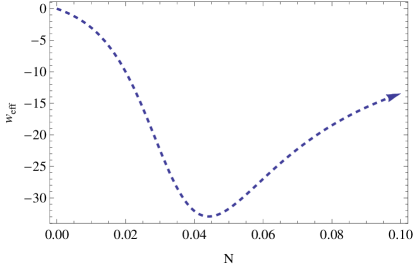
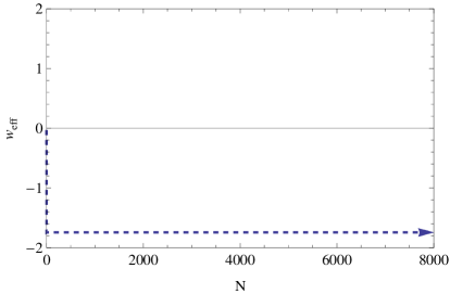
Figure 8: The evolution of the total equation of state parameter $w_{eff}$ of (38), as a function of $N$, for $c_{1}=c_{2}=1$ and $\tilde{A}=-10$.

In summary, the addition of the logarithmic corrections in the dark energy equation of state, leads either to instabilities in the phase space, or to a stable phantom fixed point at late times, and therefore to late-time acceleration. The behavior of the dynamical system for the cases X and XI is similar to the case IX, and thus we omit it for brevity. It is important to note that this model is just a simple model containing a logarithmic dependence, and in principle a more viable model can be achieved by appropriately modifying the EoS. In particular, more realistic equations of state for the dark energy fluid can be chosen, for example including polynomial terms along with the logarithmic correction.

VI Conclusions

In this work we have studied dark energy scenarios which involve equation of states with logarithmic terms of the energy density, allowing additionally for a bulk viscosity. The logarithmic-corrected power-law fluid possesses properties analogous to properties of isotropic deformation of crystalline solids, in which the pressure can be negative. Without loss of generality, we considered two classes of the model, arisen from two different viscosity considerations. In both scenarios we were able to obtain the accelerating expansion of the late Universe, since we acquired the transition from a decelerating phase to an accelerating one, without the explicit consideration of a cosmological constant.

In order to obtain a better picture of the phenomenology of the construction, we performed a confrontation with observations, and in particular with the Supernovae type Ia (SN Ia) and $H(z)$ Hubble function data, constructing the model parameter contour plots. As we showed, for both models the agreement with the is excellent, as a result of both the logarithmic correction as well as of the viscosity terms.

Additionally, we applied the powerful method of dynamical system analysis in order to extract information about the global behavior of the cosmological scenario at hand, bypassing the complexity of the involved equations, where for generality we also considered an interaction between the dark energy and matter fluids. By appropriately choosing the dimensionless variables we constructed an autonomous dynamical system, and we investigated its dynamical evolution for various parameter values and for several initial conditions. As we showed, there exist asymptotic accelerating attractors, which in most cases correspond to a phantom late-time evolution. However, in some cases it is possible to obtain a nearly de Sitter late-time evolution by appropriately choosing the model parameters, which is a significant capability of the scenario since the dark energy, although dynamical, stabilizes at the cosmological constant value.

In summary, fluids with logarithmic equation of state may lead to interesting cosmological behavior, and thus they can be a good candidate for the description of the dark energy sector. Definitely, an important and necessary investigation is to analyze in detail the cosmological perturbations, and confront them with the observed large scale structure behavior. However, this study lies outside the scope of the present work, and it is left for a future project.

References

- (1) A. G. Riess et al. [Supernova Search Team], Astron. J. 116, 1009 (1998), [astro-ph/9805201].
- (2) S. Perlmutter et al. [Supernova Cosmology Project Collaboration], Astrophys. J. 517, 565 (1999) [astro-ph/9812133].
- (3) E. J. Copeland, M. Sami and S. Tsujikawa, Int. J. Mod. Phys. D 15, 1753 (2006), [hep-th/0603057].
- (4) Y. F. Cai, E. N. Saridakis, M. R. Setare and J. Q. Xia, Phys. Rept. 493, 1 (2010), [arXiv:0909.2776 [hep-th]].
- (5) V. K. Oikonomou, J. D. Vergados and C. C. Moustakidis, Nucl. Phys. B 773 (2007) 19, [hep-ph/0612293].
- (6) J. Dutta, W. Khyllep, E. N. Saridakis, N. Tamanini and S. Vagnozzi, JCAP 1802 (2018) 041, [arXiv:1711.07290 [gr-qc]].
- (7) L. Sebastiani, S. Vagnozzi and R. Myrzakulov, Adv. High Energy Phys. 2017 (2017) 3156915, [arXiv:1612.08661 [gr-qc]].
- (8) G. G. L. Nashed, Int. J. Geom. Meth. Mod. Phys. 15 (2018) no.09, 1850154.
- (9) P. J. E. Peebles and B. Ratra, Rev. Mod. Phys. 75, 559 (2003), [astro-ph/0207347].
- (10) V. Sahni and A. A. Starobinsky, Int. J. Mod. Phys. D 9, 373 (2000), [astro-ph/9904398].
- (11) M. Li, X. D. Li, S. Wang and Y. Wang, Commun. Theor. Phys. 56, 525 (2011), [arXiv:1103.5870 [astro-ph.CO]].
- (12) J. D. Barrow and J. P. Mimoso, Phys. Rev. D 50 (1994) 3746.
- (13) C. G. Tsagas and J. D. Barrow, Class. Quant. Grav. 15 (1998) 3523, [gr-qc/9803032].
- (14) T. Buchert, Gen. Rel. Grav. 33 (2001) 1381, [gr-qc/0102049].
- (15) J. c. Hwang and H. Noh, Class. Quant. Grav. 19 (2002) 527, [astro-ph/0103244].
- (16) D. Carturan and F. Finelli, Phys. Rev. D 68 (2003) 103501, [astro-ph/0211626].
- (17) G. M. Kremer, Phys. Rev. D 68 (2003) 123507, [gr-qc/0309111].
- (18) V. Gorini, A. Kamenshchik, U. Moschella, V. Pasquier and A. Starobinsky, Phys. Rev. D 72 (2005) 103518, [astro-ph/0504576].
- (19) S. Capozziello, S. Nojiri, S. D. Odintsov and A. Troisi, a Phys. Lett. B 639 (2006) 135, [astro-ph/0604431].
- (20) W. S. Hipolito-Ricaldi, H. E. S. Velten and W. Zimdahl, JCAP 0906 (2009) 016, [arXiv:0902.4710 [astro-ph.CO]].
- (21) E. Elizalde and D. Saez-Gomez, Phys. Rev. D 80 (2009) 044030, [arXiv:0903.2732 [hep-th]].
- (22) N. Cruz, S. Lepe and F. Pena, Phys. Lett. B 699 (2011) 135.
- (23) A. B. Balakin and V. V. Bochkarev, Phys. Rev. D 87 (2013) no.2, 024006, [arXiv:1212.4094 [gr-qc]].
- (24) I. Brevik and A. V. Timoshkin, Int. J. Geom. Meth. Mod. Phys. 14 (2017) no.04, 1750061, [arXiv:1612.06689 [gr-qc]].
- (25) I. Brevik, E. Elizalde, S. D. Odintsov and A. V. Timoshkin, Int. J. Geom. Meth. Mod. Phys. 14 (2017) no.12, 1750185, [arXiv:1708.06244 [gr-qc]].
- (26) V. K. Oikonomou, Int. J. Mod. Phys. D 26 (2017) no.10, 1750110, [arXiv:1703.09009 [gr-qc]].
- (27) I. Brevik, O. Gron, J. de Haro, S. D. Odintsov and E. N. Saridakis, Int. J. Mod. Phys. D 26 (2017) no.14, 1730024, [arXiv:1706.02543 [gr-qc]].
- (28) E. Elizalde and M. Khurshudyan, arXiv:1711.01143 [gr-qc].
- (29) I. Brevik, V. V. Obukhov and A. V. Timoshkin, arXiv:1805.01258 [gr-qc].
- (30) S. Nojiri and S. D. Odintsov, Phys. Rev. D 72, 023003 (2005), [hep-th/0505215].
- (31) S. Nojiri and S. D. Odintsov, Phys. Lett. B 639, 144 (2006), [hep-th/0606025].
- (32) E. Elizalde, S. Nojiri, S. D. Odintsov and P. Wang, Phys. Rev. D 71, 103504 (2005), [hep-th/0502082].
- (33) S. Nojiri, S. D. Odintsov and V. K. Oikonomou, Phys. Rept. 692 (2017) 1, [arXiv:1705.11098 [gr-qc]].
- (34) S. Nojiri, S.D. Odintsov, Phys. Rept. 505, 59 (2011), [arXiv:1011.0544 [gr-qc]].
- (35) S. Nojiri, S.D. Odintsov, eConf C0602061, 06 (2006) [Int. J. Geom. Meth. Mod. Phys. 4, 115 (2007)].
- (36) S. Capozziello, M. De Laurentis, Phys. Rept. 509, 167 (2011), [arXiv:1108.6266 [gr-qc]].
- (37) V. Faraoni and S. Capozziello, Fundam. Theor. Phys. 170 (2010).
- (38) A. de la Cruz-Dombriz and D. Saez-Gomez, Entropy 14 (2012) 1717, [arXiv:1207.2663 [gr-qc]].
- (39) G. J. Olmo, Int. J. Mod. Phys. D 20 (2011) 413, [arXiv:1101.3864 [gr-qc]].
- (40) Y. F. Cai, S. Capozziello, M. De Laurentis and E. N. Saridakis, Rept. Prog. Phys. 79, no. 10, 106901 (2016), [arXiv:1511.07586 [gr-qc]].
- (41) H. Anton, P.C. Schmidt, Intermetallics. 5 (1997) 449.
- (42) B. Mayer et. al, Intermetallics. 11 (2003) 23.
- (43) A. L. Ivanovskii, Prog. Mat. Scie. 57 (2012) 1.
- (44) P. H. Chavanis, Eur. Phys. J. Plus 130, 181 (2015).
- (45) P. H. Chavanis, Phys. Lett. B 758, 59 (2016).
- (46) P. Gondolo and K. Freese, Phys. Rev. D 68 (2003) 063509, [hep-ph/0209322].
- (47) G. R. Farrar and P. J. E. Peebles, Astrophys. J. 604 (2004) 1, [astro-ph/0307316].
- (48) R. G. Cai and A. Wang, JCAP 0503 (2005) 002, [hep-th/0411025].
- (49) B. Wang, J. Zang, C. Y. Lin, E. Abdalla and S. Micheletti, Nucl. Phys. B 778 (2007) 69, [astro-ph/0607126].
- (50) O. Bertolami, F. Gil Pedro and M. Le Delliou, Phys. Lett. B 654 (2007) 165, [astro-ph/0703462].
- (51) X. m. Chen, Y. g. Gong and E. N. Saridakis, JCAP 0904, 001 (2009), [arXiv:0812.1117 [gr-qc]].
- (52) J. H. He and B. Wang, JCAP 0806 (2008) 010, [arXiv:0801.4233 [astro-ph]].
- (53) J. Valiviita, E. Majerotto and R. Maartens, JCAP 0807 (2008) 020, [arXiv:0804.0232 [astro-ph]].
- (54) B. M. Jackson, A. Taylor and A. Berera, Phys. Rev. D 79 (2009) 043526, [arXiv:0901.3272 [astro-ph.CO]].
- (55) M. Jamil, E. N. Saridakis and M. R. Setare, Phys. Rev. D 81 (2010) 023007, [arXiv:0910.0822 [hep-th]].
- (56) J. H. He, B. Wang and E. Abdalla, Phys. Rev. D 83 (2011) 063515, [arXiv:1012.3904 [astro-ph.CO]].
- (57) C. G. Boehmer, G. Caldera-Cabral, R. Lazkoz and R. Maartens, Phys. Rev. D 78 (2008) 023505, [arXiv:0801.1565 [gr-qc]].
- (58) K. Bamba, S. Capozziello, S. Nojiri and S. D. Odintsov, Astrophys. Space Sci. 342 (2012) 155, [arXiv:1205.3421 [gr-qc]].
- (59) Y. L. Bolotin, A. Kostenko, O. A. Lemets and D. A. Yerokhin, Int. J. Mod. Phys. D 24 (2014) no.03, 1530007, [arXiv:1310.0085 [astro-ph.CO]].
- (60) A. A. Costa, X. D. Xu, B. Wang, E. G. M. Ferreira and E. Abdalla, Phys. Rev. D 89 (2014) no.10, 103531, [arXiv:1311.7380 [astro-ph.CO]].
- (61) R. C. Nunes, S. Pan and E. N. Saridakis, Phys. Rev. D 94, no. 2, 023508 (2016), [arXiv:1605.01712 [astro-ph.CO]].
- (62) S. D. Odintsov and V. K. Oikonomou, Phys. Rev. D 97 (2018) no.12, 124042, [arXiv:1806.01588 [gr-qc]].
- (63) S. D. Odintsov and V. K. Oikonomou, Phys. Rev. D 98 (2018) no.2, 024013, [arXiv:1806.07295 [gr-qc]].
- (64) S. Capozziello, R. D’Agostino and O. Luongo, Phys. Dark Univ. 20, 1 (2018), [arXiv:1712.04317 [gr-qc]].
- (65) P. H. Chavanis and S. Kumar, JCAP 1705, no. 05, 018 (2017), [arXiv:1612.01081 [astro-ph.CO]].
- (66) R. R. Caldwell, Phys. Lett. B 545, 23 (2002), [astro-ph/9908168].
- (67) R. R. Caldwell, M. Kamionkowski and N. N. Weinberg, Phys. Rev. Lett. 91, 071301 (2003), [astro-ph/0302506].
- (68) V. Faraoni, Int. J. Mod. Phys. D 11, 471 (2002), [astro-ph/0110067].
- (69) S. Nojiri and S. D. Odintsov, Phys. Lett. B 562, 147 (2003), [hep-th/0303117].
- (70) J. D. Barrow, Class. Quant. Grav. 21, L79 (2004), [gr-qc/0403084].
- (71) S. Nojiri and S. D. Odintsov, Phys. Lett. B 595, 1 (2004), [hep-th/0405078].
- (72) S. Nojiri, S. D. Odintsov and S. Tsujikawa, Phys. Rev. D 71, 063004 (2005), [hep-th/0501025].
- (73) N. Suzuki et al., Astrophys. J. 746, 85 (2012), [arXiv:1105.3470 [astro-ph.CO]].
- (74) O. Farooq, F. R. Madiyar, S. Crandall and B. Ratra, Astrophys. J. 835, no. 1, 26 (2017), [arXiv:1607.03537 [astro-ph.CO]].
- (75) S. Capozziello, R. D’Agostino and O. Luongo, Mon. Not. Roy. Astron. Soc. 476, no. 3, 3924 (2018), [arXiv:1712.04380 [astro-ph.CO]].
- (76) S. Capozziello, Ruchika and A. A. Sen, arXiv:1806.03943 [astro-ph.CO].
- (77) S. Basilakos, S. Nesseris, F. K. Anagnostopoulos and E. N. Saridakis, JCAP 1808, no. 08, 008 (2018), [arXiv:1803.09278 [astro-ph.CO]].
- (78) A. G. Riess et al., Astrophys. J. 826, no. 1, 56 (2016), [arXiv:1604.01424 [astro-ph.CO]].
- (79) R. Adam et al. [Planck Collaboration], Astron. Astrophys. 594, A1 (2016), [arXiv:1502.01582 [astro-ph.CO]].
- (80) G. Leon and C. R. Fadragas, Cosmological Dynamical Systems, LAP LAMBERT Academic Publishing, (2011), arXiv:1412.5701 [gr-qc].
- (81) S. Bahamonde, C. G. Böhmer, S. Carloni, E. J. Copeland, W. Fang and N. Tamanini, arXiv:1712.03107 [gr-qc].
- (82) E. J. Copeland, A. R. Liddle and D. Wands, Phys. Rev. D 57, 4686 (1998), [gr-qc/9711068].
- (83) G. Leon and E. N. Saridakis, JCAP 0911, 006 (2009), [arXiv:0909.3571 [hep-th]].
- (84) G. Leon and E. N. Saridakis, Class. Quant. Grav. 28, 065008 (2011), [arXiv:1007.3956 [gr-qc]].
- (85) G. Kofinas, G. Leon and E. N. Saridakis, Class. Quant. Grav. 31, 175011 (2014), [arXiv:1404.7100 [gr-qc]].
- (86) S. D. Odintsov and V. K. Oikonomou, Phys. Rev. D 96 (2017) no.10, 104049, [arXiv:1711.02230 [gr-qc]].
- (87) V. K. Oikonomou, Int. J. Mod. Phys. D 27 (2018) no.05, 1850059, [arXiv:1711.03389 [gr-qc]].
- (88) K. Kleidis and V. K. Oikonomou, arXiv:1808.04674 [gr-qc].
- (89) G. Caldera-Cabral, R. Maartens and L. A. Urena-Lopez, Phys. Rev. D 79 (2009) 063518, [arXiv:0812.1827 [gr-qc]].
- (90) D. Pavon and W. Zimdahl, Phys. Lett. B 628 (2005) 206, [gr-qc/0505020].
- (91) M. Quartin, M. O. Calvao, S. E. Joras, R. R. R. Reis and I. Waga, JCAP 0805 (2008) 007, [arXiv:0802.0546 [astro-ph]].
- (92) H. M. Sadjadi and M. Alimohammadi, Phys. Rev. D 74 (2006) 103007, [gr-qc/0610080].
- (93) W. Zimdahl, Int. J. Mod. Phys. D 14 (2005) 2319, [gr-qc/0505056].