Chiara Lepore \extraaffilLamont-Doherty Earth Observatory, Columbia University, Palisades, New York \extraauthorWilliam J. Koshak \extraaffilNASA Marshall Space Flight Center, Huntsville, Alabama \extraauthorThemis Chronis \extraaffilUniversity of Alabama in Huntsville, Huntsville, Alabama \extraauthorBrian Vant-Hull \extraaffilCity College of New York, New York City, New York
Performance of a simple proxy for U.S. cloud-to-ground lightning
Abstract
The product of convective available potential energy (CAPE) and precipitation rate has previously been used as a proxy for cloud-to-ground (CG) lightning flash counts in climate change applications. Here the ability of this proxy, denoted CP, to represent the climatology and variability of CG lightning flash counts over the contiguous U.S. (CONUS) during the period 2003–2016 is assessed. CP values computed using the North American Regional Reanalysis are compared with negative and positive polarity CG flash counts from the National Lightning Detection Network. Overall, the proxy performs better on shorter time scales (daily and monthly) than on longer time scales (annual and semi-annual). Proxy performance tends to be worse during the warm season (May–October), when most lightning occurs, and better during the cool season (November–April). The correlation of annually accumulated CONUS CP with CG flash counts is not statistically significant because of poor warm-season performance. Cool season negative CG flash counts are well-correlated with CONUS CP values. Positive CG flash counts (7% of all CG flashes) are well correlated with annual values of CONUS CP. The relatively strong relations between CP and CG flash counts in some regions and times of the year at daily resolution provide a benchmark for more complex proxies and suggest that proxy-based extended- and long-range prediction of lightning activity may be feasible to the extent that precipitation rate and CAPE can be predicted.
1 Introduction
Lightning flash rate is a defining characteristic of thunderstorm evolution. Cloud-to-ground (CG) lightning impacts societies through deaths and injuries, property damage, wildfires, and air quality (Koshak et al. 2015). The importance of CG lightning is a motivation for studying how its characteristics vary under climate change and variability. The relation of lightning with climate, whether in the form of interannual variability or long-term trends, is difficult to infer directly from the observational record because high-quality, spatially-complete lightning datasets are often relatively short. Moreover, observational data can at best provide circumstantial information about expected lightning characteristics in climates that differ from the one in which observations are collected, be they future climates or ones in other regions.
Lightning activity in general depends on the dynamics and microphysics of convective clouds, and this dependence has been modeled with varying levels of detail and complexity. Lightning occurrence and flash rates can be simulated with considerable fidelity and realism by combining electrification and lightning parameterizations with models of atmospheric dynamics and microphysics (Mansell et al. 2005; Kuhlman et al. 2006; Fierro et al. 2013). Lightning rates have also been related in a more empirical but effective manner to cloud properties, microphysical parameters, and updrafts generated by convection permitting models (McCaul et al. 2009; Yair et al. 2010; Lynn et al. 2012). Alternatively, lightning flash densities can be diagnosed from the output of convective parameterization schemes in models that do not explicitly resolve clouds (Allen and Pickering 2002; Lopez 2016). Stolz et al. (2017) parameterized storm-scale total lightning density using environmental variables from reanalysis and aerosol data.
However, detailed cloud and microphysical properties are not always readily available from reanalysis, seasonal forecasts, or climate change projections, and are themselves uncertain. Therefore, simple proxies for lightning that depend on a few, easily available quantities may provide utility for climate variability and projection applications. Romps et al. (2014) proposed the product of convective available potential energy (CAPE) and total precipitation rate as a proxy for the number of total CG lightning flashes. The application of this proxy to climate change projections predicts a 50% increase in United States lightning strokes over the 21st century. An attractive feature of the Romps proxy is that there is some theoretical understanding of how its constituents are modulated by short-term climate variability (e.g., ENSO; Ropelewski and Halpert 1987; L’Heureux et al. 2015; Allen et al. 2015b) and long-term change (Held and Soden 2006; Seeley and Romps 2016). Also, its ingredients are standard outputs of many seasonal and subseasonal dynamical forecasting systems and could be used to make extended-range forecasts of lightning activity (Dowdy 2016; Muñoz et al. 2016). Analogous approaches have been used to relate tornado and hail activity with nearby meteorological quantities at monthly and daily resolution (Tippett et al. 2012; Allen et al. 2015a; Tippett et al. 2016; Westermayer et al. 2017). A caveat of empirical proxy-based approaches is that good performance in the current climate does not guarantee good performance in future climates (Stainforth et al. 2007; Camargo et al. 2014).
The goal of this work is to assess the extent to which the ingredients of the Romps proxy, precipitation rate and CAPE, capture recent variability in CG flash counts over the contiguous United States (CONUS). Of course, assessing the performance of the proxy in capturing observed CG flash counts is a necessary, but not sufficient requirement for its use in applications such as climate projections and subseasonal to seasonal (S2S) predictions, which is our long-term goal. Importantly, good performance with reanalysis in no way guarantees comparable performance in climate projection or S2S forecast applications. On the other hand, poor performance of the proxy in reanalysis would provide useful indications of its limitations. Also, the choice of the Romps proxy is motivated by the availability of CAPE and total precipitation rate in forecast and reforecast datasets such as those of the NOAA Climate Forecast System, version 2 (Saha et al. 2014; Lepore et al. 2018), the S2S Prediction Project Database (Vitart et al. 2016), and the Subseasonal Experiment (SubX) database (Pegion et al. 2018). However, the CAPE values that are available from forecast models can be sensitive to the choice of parcel and use of the virtual temperature correction.
Romps et al. (2014) showed a strong association between daily counts of total CONUS CG flashes and the product of CONUS-averages of precipitation rate and CAPE during a singer year, 2011. Here we use a longer period (14 years) and to see what additional years of data can tell us about seasonal variations in the strength of the association and about the ability of the proxy to capture interannual variability in CG flash counts. Romps et al. (2014) used CAPE calculated from radiosonde data and a NOAA River Forecast Centers precipitation product based on rain-gauge and radar data. Here we test the quality of the association between CG flash counts and the CAPE-precipitation product when reanalysis products are used instead of solely observation-based ones. Knowing whether or not reanalysis products are sufficiently realistic for this purpose is important because it helps to judge whether such a climate proxy computed from numerical model outputs can be used to forecast or project future CG lightning activity. Furthermore, the use of spatially complete reanalysis data allow us to form the product of collocated CAPE and precipitation rate (denoted CP) on a spatially resolved grid and to examine regional features of the association of the CAPE-precipitation product with CG lightning flash counts.
2 Data and methods
2.1 Data
We use precipitation rate (mm d-1) and 0-180 hPa most unstable CAPE (J kg-1) data from the North American Regional Reanalysis (NARR; Mesinger and Coauthors 2006). The most unstable parcel is found by dividing the 0-180 hPa layer into six 30-hPa-deep layers and selecting the one with the largest equivalent potential temperature (no virtual temperature correction). NARR data are provided at 3-hourly resolution. The precipitation rate is based on a 3-hour accumulation. CAPE is the instantaneous value at the start of the 3-hour period. The data are averaged from their 32 km native grid spacing to a latitude-longitude grid. We choose the 1-degree grid spacing to match that of CFSv2 and SubX data because our long-term goal is S2S prediction. NARR precipitation estimates show some advantage over ones from other reanalysis products, especially global reanalysis, likely due to its use of precipitation observations which it assimilates as latent heating profiles (Bukovsky and Karoly 2007; Cui et al. 2017).
Cloud-to-ground (CG) lightning flash counts come from the National Lightning Detection Network (NLDN; Cummins and Murphy 2009) and are summed on the same grid at daily (UTC) resolution. Only CONUS land points are used in our analysis although both NARR and NLDN data extend over ocean and into Mexico and Canada. We use NLDN data covering the period 2003–2016 (5114 days) during which the NLDN network is complete and stable (Koshak et al. 2015). There are 9 days with missing NLDN data: 31/12/03, 08/02/04, 08/02/06, 16/01/07, 06/02/07, 18/12/07, 05/12/08, 17/01/09, 16/01/13, and those days are excluded from calculations. A change in the NLDN Total Lightning Processor (TLP) on 18/09/15 may be responsible for a substantial increase noted in the number of positive CG flashes reported during 2016 (Nag et al. 2016).
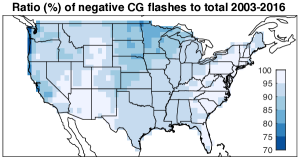
Negative and positive ( 15 kiloampere; kA) polarity CG lightning flash counts are analyzed separately to examine whether the proxy performance differs for positive and negative flash counts. Differing proxy performance might be expected since environment, at least at the mesoscale, can affect storm structure and CG flash polarity (Carey and Buffalo 2007). Total CG flashes were also analyzed but give results that are very similar to those for negative CG flash counts. The threshold of 15 kA for positive polarity flashes accounts for the tendency of the NLDN to misclassify cloud pulses as low-amplitude, positive CG strokes (Biagi et al. 2007; Cummins and Murphy 2009). The new NLDN TLP removes the 15 kA peak current limit for positive CG flashes. Therefore, to maintain more consistency, we apply our own 15 kA filter to the positive CG flashes in 2015 and 2016. As a consequence, the numbers of positive CG flashes analyzed here for 2015 and 2016 are less than those in the unfiltered NLDN data sets. The majority (93%) of CONUS CG flashes have negative polarity during the period 2003–2016. The ratio of negative polarity CG flashes to total CG flashes shows substantial spatial variations (Fig. 1), with ratios above 95% on the Eastern Seaboard, below 85% in the Upper Midwest and the lowest values in very narrow band along the West Coast, consistent with the patterns found in individual years Koshak et al. (2015). Positive polarity CG flashes have been associated with severe thunderstorms in the Midwest (tornadoes, hail, and damaging wind; e.g., MacGorman and Burgess 1994; Carey and Rutledge 2003). However, other regions with frequent severe weather do not show especially elevated percentages of positive CG flashes. Conversely, the high percentages of positive CG flashes along the West Coast occur where severe weather is infrequent (Zajac and Rutledge 2001; Koshak et al. 2015; Medici et al. 2017).
Here we use the product of collocated 3-hourly values of CAPE and precipitation rate as a proxy for the number of CG flashes that occur during those three hours in the corresponding grid cells, and we denote this quantity as CP. Using a proxy based on collocated values allows us to compare it with CG flash counts on a regional as well as CONUS-wide basis. Three-hourly CP values are summed over time to form daily, monthly, seasonal, and annual values; they are summed over space to form regional CONUS values. CP values are scaled to facilitate their comparison with CG flash counts. The scaling factor is computed so that the area-weighted sum of CP values over the period 2003–2016 matches the number of CONUS flashes, depending on polarity. In other words,
The scaling factor for negative polarity CG flashes is 64.17 flashes / J kg-1 mm day-1 and 4.79 flashes / J kg-1 mm day-1 for positive polarity CG flashes. On the grid,
and
where is latitude in radians, and accounts for the varying grid cell area. The same scaling factor is used in all months and locations. All comparisons between CP and CG flashes use scaled CP, and we drop the word scaled hereafter.
2.2 Methods
We assess regional behavior by spatially aggregating CP and CG flashes at the level of NOAA climate regions (Karl and Koss 1984). The states in each region are listed in Table 1. The spatial structure of CP and CG flashes are compared using pattern correlations computed for the points east of 105∘W with the map mean removed (Wilks 2011). The pattern correlations are computed using points east of 105∘W to focus on the region where the vast majority of CG flashes are recorded and to avoid giving credit for simply matching the east-west gradient. The temporal association between CP and CG flashes is measured using correlation and mean-squared error (MSE), where the error is the difference of CP and the number of CG flashes. MSE is normalized by the CG flash variance (at the same temporal resolution) to allow comparison of error levels for regions and seasons with disparate levels of CG flash activity. In addition to daily, monthly, and annual aggregation, we also look at totals for six-month warm (May–October) and cool (November–April) seasons, with the cool season comprising the 13 complete seasons 2003/2004–2015/2016 for which data are available. For interannual correlations (14 years), the critical correlation value at the 5% significance level for rejecting the null hypothesis of no correlation is about 0.46 for a one-tailed test and 0.53 for a two-tailed test.
3 Results
3.1 Regional scaling of CP and CG flashes
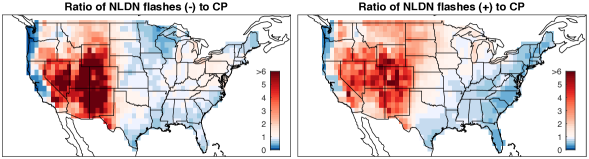
Although CP is scaled to match the CONUS total of CG flashes, the ratio of CG flashes to CP shows distinct regional variations (Fig. 2), which presumably reflect the differing frequency of rainfall processes and cloud properties that are not accounted for in CP. Also, the spatial variations in the ratio of CG flashes to CP may indicate a role for additional thermodynamic factors such as wet-bulb temperature (Koshak et al. 2015), mid-level humidity (Westermayer et al. 2017) or warm cloud depth (Stolz et al. 2017). Values of the ratio of negative CG flashes to CP are slightly above one in the Northeast, where aerosol concentrations are relatively large (van Donkelaar et al. 2015). The ratio of negative flashes to CP is near one east of the Rockies, substantially greater than one west of 105∘W, until along the West Coast where the ratio is much less than one. The picture for positive CG flashes is similar, but without elevated ratio values in the Northeast and with a stronger gradient from values greater than one in the Northern Rockies and Upper Midwest to values less than one in the Southeast. The single scaling factor applied to CP for each polarity matches the behavior in the East because 91.0% of the negative polarity CG flashes and 93.4% of the positive polarity CG flashes occur east of 105∘W. Previous studies have noted that ice-based precipitation processes are dominant in the arid Southwestern US, and the ratio of convective rainfall to lightning (rainfall yield) is relatively low there (Petersen and Rutledge 1998). Mülmenstädt et al. (2015) found that ice-phase clouds were more frequent in the western half of the CONUS and that liquid-phase clouds were more frequent east of the Rockies. Lower lifted condensation level heights in the East (not shown) are suggestive of lower cloud bases and conditions favoring warm rain processes with greater precipitation efficiency. Fuchs et al. (2015) compared total lightning flash rates in Colorado, Oklahoma, Alabama, and the District of Columbia, and hypothesized that storms with high cloud base heights or shallow warm cloud depths have less warm-phase precipitation and more mixed-phase precipitation and lightning. The low ratio of CG flash count to CP in a narrow band along the West Coast may be related to onshore flow of maritime air masses with fewer cloud condensation nuclei or dynamically weaker convection that develops offshore and at coastal boundaries (Zipser 1994; Xu et al. 2012; Holle et al. 2016). Despite some regional scaling deficiencies, CP matches CG flash counts relatively well in the areas where the vast majority of CONUS CG lightning occurs.
3.2 Daily associations of CONUS totals
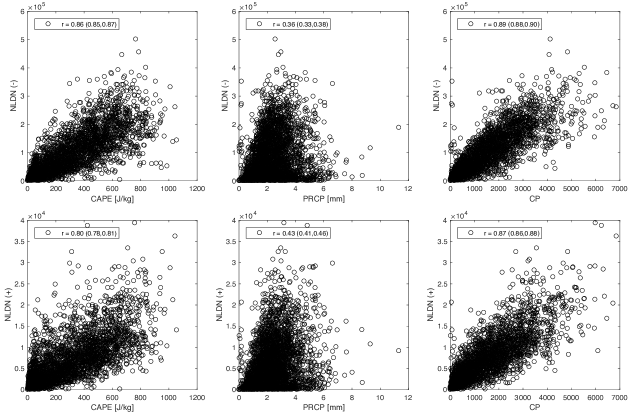
We first consider the association of daily CONUS CG flash counts with CAPE alone. The correlation of daily CONUS CG flash counts with CONUS-averaged CAPE from NARR over the period 2003–2016 is larger (values of 0.86 and 0.8, respectively, for counts of negative and positive CG flashes; Fig. 3) than that found by Romps et al. (2014) for CAPE computed from radiosonde data for the single year 2011 (). In fact, there is some expectation that reanalysis CAPE might be more representative of large-scale features than would be CAPE computed from radiosonde data, since radiosonde data contain small-scale variability that may not be representative of the large-scale nearby environment. Lepore et al. (2016) found a stronger relation between gauge-measured rainfall extremes and CAPE from reanalysis than with CAPE based on nearby radiosonde measurements. Also, the use of time-averaged reanalysis CAPE and precipitation possibly mitigates the difficulty of using observed collocated CAPE and precipitation that is caused by CAPE being released by convection (Romps et al. 2014). On the other hand, daily CONUS-averaged precipitation from NARR shows a slightly weaker relation with CG flash counts (correlation values of 0.36 and 0.43 for negative and positive CG flash counts, respectively; Fig. 3) than the reported by Romps et al. (2014) using a NOAA River Forecast Centers precipitation product based on rain-gauge and radar data. Daily CONUS CP has a slightly stronger relation with flash counts (correlation values of 0.89 and 0.87 for negative and positive polarity, respectively; Fig. 3) than does CAPE alone. We note that including precipitation rate has the potential to introduce some dependence on aerosols since rain rate increases with aerosol level (Koren et al. 2012).
3.3 Annual cycle and climatology
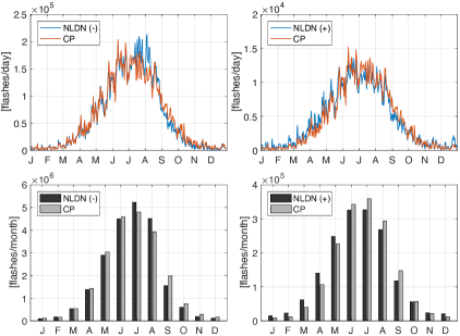
CONUS CP and CG flash counts have strikingly similar annual cycles, both at daily and monthly resolution, with peak values in summer and much smaller values in the cool season (Fig. 4). The increase in CG occurrence from spring to summer is gradual and followed by a somewhat sharper decay after August (Holle et al. 2016). Annual cycles at daily resolution are computed by averaging the 14 values (2003–2016) available for each calendar day with February 29 excluded. The daily resolution annual cycle shows that CONUS CP appears to resolve some sub-monthly features that are likely specific to this set of years. The largest discrepancy between the annual cycles of CONUS CP and negative CG flash counts (clearest at monthly resolution) occurs in July–August when CP values are too low and in September–October when CP values are too high (Fig. 4). There is also good agreement between the annual cycles of CONUS CP and positive CG flash counts, with a tendency of CP values to be too low in spring (March–May) and too high in summer and early fall (June–September).
The similarity of the annual cycles of CONUS CP and CG flash counts means that some of the variance of CG flash counts at daily resolution explained by CP (Fig. 3) is a consequence of CP accurately capturing the seasonality of CG flash counts. In fact, the annual cycle of CP at daily resolution, a quantity with no year-to-year variation, explains 63% and 52% of the variance of negative and positive daily CONUS CG flash counts, respectively. The annual cycle of CP at daily resolution explains nearly as much variance of daily negative and positive CONUS CG flash counts as do their own annual cycles, which explain 66% and 54%, respectively.
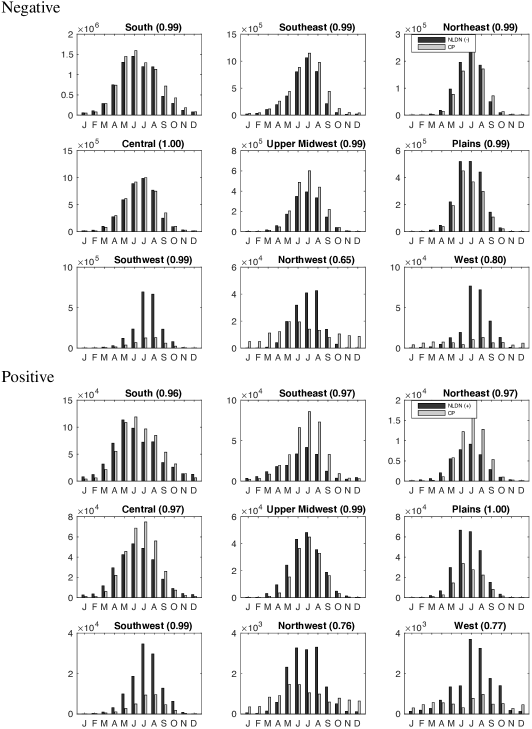
CP captures the annual cycle of lightning occurrence at the regional level and monthly resolution to varying degrees (Fig. 5). Because a single (polarity-dependent) factor is used to scale CP, the differing performance of CP in matching the relative magnitude and phasing of the regional seasonal cycles provides another indication of the extent to which CAPE and precipitation alone are adequate to provide a statistical description of CG flash counts. For the most part, both the magnitude of the CG annual cycle and its phasing are well-matched by that of CP in regions east of the Rockies. Because the majority of lightning flashes occur in the eastern half of the country, the scaling factor is disposed to match the magnitude there. In the Upper Midwest, where the ratio of positive to negative CG flashes is relatively large, the CP annual cycle is stronger than that of the negative CG flashes, and better matches the annual cycle magnitude of the positive CG flashes. CP overestimates negative CG flashes in the Upper Midwest during July–August and underestimates them in the Plains. The largest differences in annual cycle magnitude are present in the Southwest, Northwest, and West regions where CP is substantially too low compared to both negative and positive CG flash counts. These annual cycle biases indicate that a lightning proxy could potentially benefit from taking into account physical factors that are different in these regions (e.g., warm cloud depth) and that are not captured by reanalysis precipitation and CAPE. Alternatively, regionally-varying, empirical corrections could be applied to CP as is done to the output of numerical weather and climate prediction models.
CP shows the largest phase errors in the Northwest and West. CP in the Northwest peaks in May–June while CG flash counts peak in June–August and have stronger seasonality (greater peak to trough differences). In the West, CP shows a bimodal structure with a peak in August and a secondary peak in early spring, while CG flash counts have a unimodal distribution with a peak in July and stronger seasonality. CP tends to match the annual cycle of positive CG flashes less well than it does negative ones, especially in the Southeast, Northeast and Central regions where CP overestimates the peak magnitude.
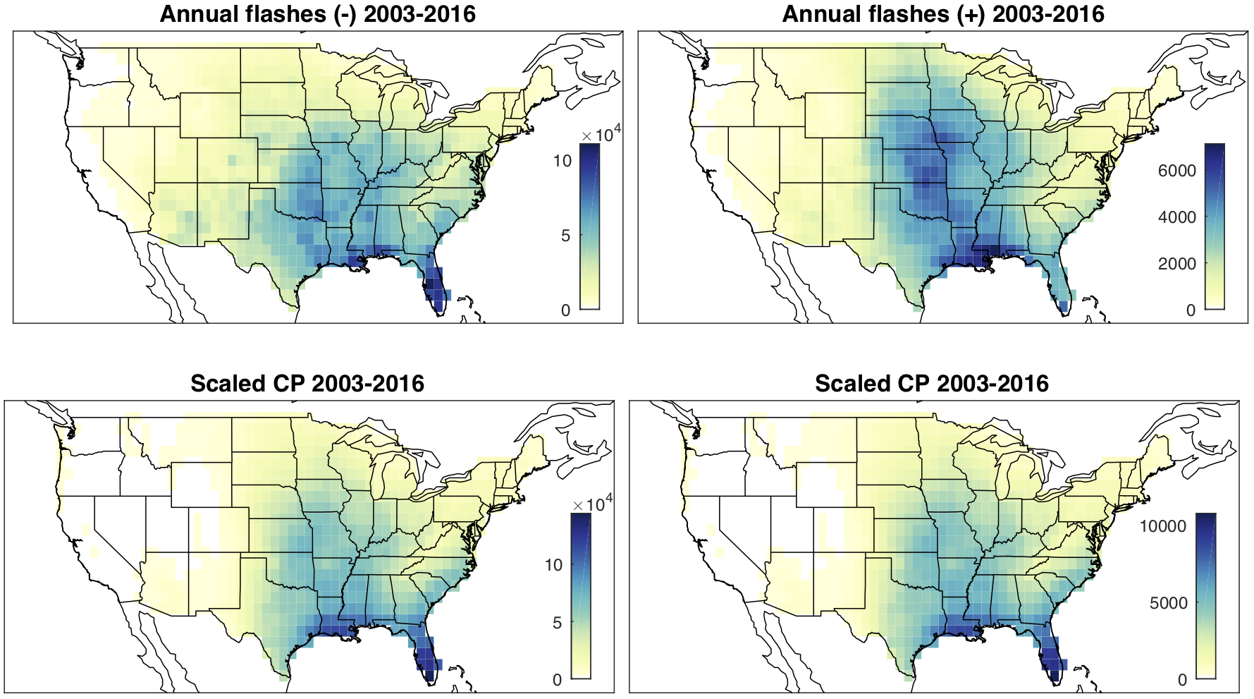
The annual spatial distribution of CP is more similar to that of negative CG flashes than that of positive CG flashes (Fig. 6). The annual spatial distribution of negative CG flashes is nearly indistinguishable from all CG flashes (not shown). Compared to counts of positive CG flashes, corresponding CP values are too low in the middle of the CONUS (Oklahoma, Kansas, and Nebraska) and too large along the Southeast coast, and over Florida. Centered pattern correlations between the climatological monthly maps of NLDN flash counts and the CP proxy computed for the CONUS region east of 105∘W show good agreement for negative polarity flashes throughout the year, but are relatively poor for positive CG flashes during June–October (Table 2), which are months when CP values tend to be too high in the Southeast, Northeast, and Central regions and too low in the Plains region (Fig. 5).
3.4 Seasonality in the strength of daily associations
We compute the correlation between daily CONUS CG flash counts and CP values for each of the twelve calendar months separately to examine how the strength of the association between daily CP values and flash counts varies through the calendar. By removing the mean of each calendar month from the daily data, we remove much of the contribution of the annual cycle to the correlation of daily values computed in Section 33.2, though some months have considerable climatological mean changes within the month (e.g., August). The correlation between daily CONUS CP and CG flash counts by calendar month is very similar for negative, positive, and all polarity flashes (Table 3), and shows a clear seasonality with lower values in summer and fall. The median correlation between daily CONUS CP and all CG flash counts by calendar month is 0.88 during the months of November through May, while it is 0.70 during the months of June through October.
The normalized daily MSE shows a consistent picture with larger relative errors in the months of June through November (Table 3). The daily normalized MSE is relatively low during the months of November through April with a median of 24% and 36% for negative and positive CG flash counts, respectively. However, during the months of May through October, the median daily normalized MSE is 66% and 65%, respectively, for negative and positive CG flash counts. Normalized MSE values greater than one for negative CG flashes in September and October indicate that the errors are greater than would result from replacing the daily CP values with the monthly average over the period. Higher daily errors during the months of peak lightning occurrence might be expected to accumulate and limit the ability of CP to capture year-to-year variations of seasonal and annual totals.
3.5 Interannual variability
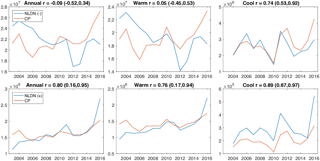
We now examine the ability of CP to match year-to-year variations in monthly, six-month, and annual values of CG flash counts. At annual resolution, there is no substantial correlation of CONUS CP with counts of negative CG flashes (; Fig. 7) or with counts of all CG flashes (, not shown). To some extent, this lack of association between annual values of CONUS CP and negative CG flashes is unexpected since daily values are well-correlated, both in an overall sense that includes seasonality, and when focusing on individual months. Time averaging often reduces noise and enhances statistical relations, but, in this case, time averaging serves to highlight deficiencies of CP during the warm season. The correlation of annual CONUS CP with counts of positive CG flashes is considerably larger (; Fig. 7), although that correlation drops to 0.52 when the largest annual value (2016) is removed. The large number of positive CG flashes recorded in 2016 could be due to the new flash type classification technique that is based on the examination of multiple waveform parameters, and that was employed within the TLP as indicated in Nag et al. (2016).
The correlation between warm season (May–October) CONUS CP and CG flashes is roughly the same as for annual values ( and for negative and positive polarity, respectively; Fig. 7). Annual counts of CG flashes are dominated by warm season values in the sense that warm season flashes account for 89% of negative CG flashes and 83% of positive CG flashes during the period 2003–2016 (Tables 4 and 5), and in the sense that warm season counts of CG flashes are highly correlated with annual values ( and , for negative and positive flashes, respectively). During the cool season (November–April), CONUS CP shows a fairly good association with negative (; Fig. 7), positive (; Fig. 7) and all (, not shown) CG flash counts. The good association of CONUS CP with the number of CG flashes of both polarities during the cool season is possible because the correlation between the number of negative and positive cool season CONUS CG flashes is 0.69. In contrast, the correlation between the number of negative and positive warm season CONUS CG flashes is -0.32.
The correlations of monthly values of CONUS CP with negative CG flashes (first line of Table 6) are considerably higher than the annual or warm season correlations, though the correlations for months during the warm season (median correlation 0.47) tend to be lower than for months during the cool season (median correlation 0.87). Correlations of positive CG flash counts with monthly CONUS CP are above 0.85 during six months of the year and fall below 0.5 only in August and October (first line of Table 7), with a tendency toward lower correlations during warm season months (median correlation 0.65) compared to cool season months (median correlation 0.87). The lower level of correlations during some warm season months is consistent with relatively low correlations and poor normalized MSE at daily resolution during warm season months noted earlier (Table 3).
At the regional level, correlations between monthly CP and negative CG flash counts are overall higher than those at the CONUS level, particularly during warm season months (May through October) when 87% of the regional correlations are greater than CONUS ones (Table 6). Lower correlation with increasing spatial aggregation is consistent with regionally varying magnitude errors. Correlations of monthly CP and negative CG flash counts show some indication of relatively lower values in warm season months in the Southeast, Northeast, and South regions, which produce more than 68% of the annual CONUS number of negative CG flashes (Table 4). Correlations of monthly CP and positive CG flash counts show some reduced values during warm season months in the South and Southeast regions (Table 7), but are otherwise fairly strong except in the Central, Upper Midwest, and Plains regions during some cool season months. Despite clear deficiencies in the South, and Southeast regions during the warm season, which likely contribute to poor CONUS performance, the relation between monthly CP and CG flash counts is strong in many regions and during many times of the year, demonstrating the strong potential for CP as an indicator of monthly tendencies in regional CG flash counts.
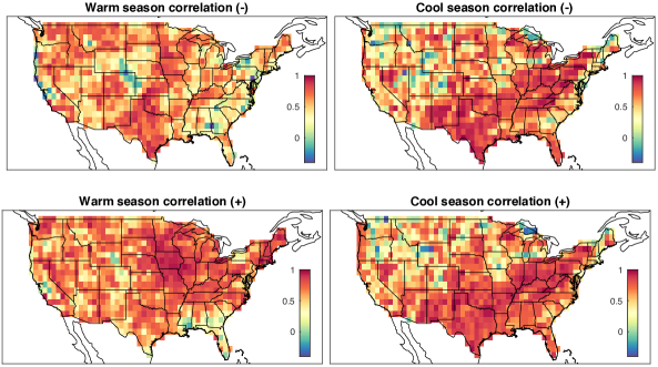
Maps of the correlation between warm and cool season CP and CG flashes show large-scale features that are consistent with the analysis at the NOAA region level, as well as fairly high correlations at the gridpoint level in many areas (Fig. 8). Correlations of warm season CP with negative CG flash counts are mostly positive, but very modest in the Southeast, Northeast, and parts of the South, consistent with the regional analysis. Correlations between warm season CP and negative CG flash counts are weakly negative in an area that includes the borders of Colorado, Wyoming, Nebraska, and Kansas where the ratio of intra-cloud lightning to CG flashes is known to be large and which is often associated with inverted or complex charge structures (Carey and Rutledge 1998; Medici et al. 2017). Misclassification of cloud pulses as CG flashes as well as incorrect assignment of first peak polarity have been noted in the Kansas-Nebraska area (Cummins and Murphy 2009). Warm season correlations between CP and negative CG flash counts are also weakly negative in smaller areas along the West Coast, and around Butte, Montana, and Columbus, Georgia. Cool season correlations between CP and CG flash counts of both polarities are similar and generally higher than warm season ones across the southeastern half of the CONUS. Correlations between warm season CP and positive CG flashes are overall higher than for negative CG flashes over most of the CONUS, with low correlations mostly limited to Florida and states to its immediate north (Fig. 8). Maps of annual correlations (not shown) are similar to those for the warm season.
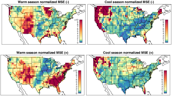
Warm season normalized MSE exceeds one in many areas for both polarities, indicating errors that are larger than the climatological variance, especially west of 105∘W where mean biases are large (Fig. 9). For negative CG flashes, the warm season normalized MSE east of the Rockies is mostly less than one except in areas that include Wisconsin and eastern Minnesota, the Gulf Coast, and eastern North Carolina. On the other hand, the warm season normalized MSE for positive CG flashes is large across the Southeast and Northeast regions, indicating magnitude miscalibration since correlations are good there (Fig. 8). The normalized cool season MSE is lower overall than the warm season MSE for both polarities, except in the Northwest and on the West Coast. Cool season normalized MSE is lower overall for negative CG flashes than for positive ones. Both polarities have large normalized MSE over southern Florida in the cool season. Annual normalized MSE maps (not shown) are similar to warm season ones.
4 Summary and discussion
We have compared the product of collocated CAPE and precipitation (denoted CP) taken from the North American Regional Reanalysis with counts of negative and positive cloud-to-ground (CG) lightning flashes from the National Lightning Detection Network (NLDN) over the contiguous U.S. (CONUS). Our analysis includes CONUS-wide and regional characteristics on daily, monthly, and annual resolution for the period 2003–2016. This analysis extends the findings of Romps et al. (2014) who considered one year of CONUS-aggregated daily values from 2011. Overall, the association of CP with lightning flashes on the daily, monthly, and seasonal scale tends to be stronger during the cool season (November–April) than during the warm season (May–October). Interannual correlations between CP and flash counts tend to be stronger for positive CG flashes than for negative ones.
Daily values of CONUS CP are highly correlated with both positive and negative CG flash counts, explaining more than 75% of their daily variance (Fig. 3). Some of this association (more than 60% of the variance) is a reflection of the strong seasonal cycles of CONUS CP and CG flash counts, and their good phase agreement (Fig. 4). However, daily variations of CONUS CP and CG flash counts with respect to their monthly climatologies are still strongly related, but with stronger associations in the cool season (November–April) than in the warm season (May–October) when most lightning occurs (Table 3). The normalized (relative to climatological variance) daily mean-squared error (MSE) of CONUS values is also larger in the warm season, and this lower accuracy translates into lower interannual correlations (Fig. 7) and higher normalized MSE for monthly totals in the warm season (Table 6), especially for negative polarity flashes, which are the vast majority of CG flashes. The low correlation in summer months might indicate that CP is better-related to storm occurrence than to the total number of CG flashes within a storm. This lack of association during the warm season when the majority of lightning occurs results in there being essentially no correlation between the annual values of CP and corresponding numbers of either negative or total CG lightning flashes. There is, however, a good correlation between warm season and annual counts of positive CG flashes with CP (Fig. 7). Cool season CP correlates well with both counts of positive and negative CG flashes.
We find that the ratio of CP to CG flash counts varies considerably on a regional basis, with the greatest difference found in the arid Southwest where the ratio of CG flashes to CP is substantially higher than in between regions east of the Rockies (Fig. 2). The ratio of CG flashes to CP is lowest along the West Coast where there are fewer cloud condensation nuclei and where maritime air masses can penetrate. At the level of NOAA climate regions, despite some errors in magnitude, CP matches the annual cycle in all regions fairly well except the Northwest and West (Fig. 5). Correlations of annual CP with CG flash counts at the regional level are generally higher for positive than for negative CG flash counts ((Tables 6 and 6). Regional correlations of annual CP and negative CG flash counts are especially low in the South and Northeast, where more than 35% of all negative CONUS CG flashes occur. The relatively weak association between CP and counts of negative CG flashes in these areas during the warm season explains the lack of correlation between annual CONUS CP and negative CG flash counts. In these regions, correlations between cool season CP and CG flash counts are generally stronger than for warm season values.
Maps of the correlation between annual values of CP and CG flash counts show positive values over most of the CONUS with some spatially limited exceptions (Fig. 8). In general, correlations with CP are stronger for positive CG flash counts and stronger during the cool season for both polarities. Despite the positive correlations at the gridpoint level, interannual variability of CP values are not well-calibrated with CG flash counts. Maps of normalized MSE show relatively low error levels for both polarities during the cool season for most of the CONUS except for large errors on the West Coast, the Northwest, and southern Florida (Fig. 9). Normalized MSE is small during the warm season for positive CG flash counts in a swath that extends from Texas northeast to the Great Lakes.
The suitability of CP for S2S forecasting cannot be concluded from this study. Further assessment with reforecast data is required (Tippett and Koshak 2018). However, in principle, the utility of CP for S2S forecasting is at least limited by its performance with reanalysis data and the extent that its constituents can be forecast. The high correlations between CP and CG flash counts across large portions of the U.S. show that this simple proxy captures considerable variability. Conversely, we have also identified regions and times of the year when CP values are not strongly correlated with CG flash counts, and this weakness suggests the need for improvements in the proxy. The degree to which CP can be predicted in advance is unknown but there are indications that its ingredients, precipitation and CAPE, can be predicted with some skill. U.S. precipitation is already forecast with current forecast systems with some skill at subseasonal (DelSole et al. 2017) and seasonal (Becker et al. 2014) time-scales. However, skill tends to be lowest in the warm season. Seasonal values of CAPE have been demonstrated to be predictable as well (Jung and Kirtman 2016). On the other hand, even in many locations where correlations between CP and CG flash counts are high, the MSE is also relatively high, indicating that the CP proxy is not calibrated to match CG flash counts. In these cases, there is the potential to correct CP values on a regional basis to match CG flash counts. Alternatively, this lack of calibration can also be interpreted as indicating that the proxy can be improved with the addition of other factors that are important for characterizing lightning activity, though perhaps at the risk of losing its attractive simplicity.
The 14 years of data used in this study are not adequate to answer fully the question of whether CP is useful proxy for long-term climate applications. Over the period of study, the annual number of CONUS CG flashes varied from a high of flashes in 2004 to a low of flashes in 2012, a range of about 35% of the annual average of flashes. However, this variation in the annual number CONUS CG flashes was not well-captured by the CP proxy. This poor performance in describing interannual variability of CONUS CG flash counts does not necessarily mean that this approach is poorly suited to climate change applications but does raise concerns and questions about the applicability of the proxy to climate change applications. Moreover, there are strong indications that CP is missing factors whose variation could be relevant for long-term lightning activity, at least as measured by CG flash counts. Finally, future work in this area should employ all lightning flashes (intra-cloud and CG), which is now possible CONUS-wide due to the recent launch of the Geostationary Lightning Mapper (GLM) on GOES-16. GLM will provide uniform, continuous total lightning observations over the Americas and surrounding ocean areas (Goodman et al. 2013).
Acknowledgements.
Valuable comments and suggestions from Ken Cummins are gratefully acknowledged. M.K.T. and C.L. were partially supported by a Columbia University Research Initiatives for Science and Engineering (RISE) award; Office of Naval Research awards N00014-12-1- 0911 and N00014-16-1-2073; NOAA’s Climate Program Office’s Modeling, Analysis, Predictions, and Projections program award NA14OAR4310185; and the Willis Research Network. We are also thankful for the support from NASA Program NNH14ZDA001N-INCA (Climate Indicators and Data Products for Future National Climate Assessments; Dr. Jack Kaye and Dr. Lucia Tsaoussi, NASA Headquarters). The authors gratefully acknowledge Vaisala Inc. for providing the NLDN data used in this study. North American Regional Reanalysis data are provided by the NOAA/OAR/ESRL PSD, Boulder, Colorado, USA from their website at http://www.esrl.noaa.gov/psd and the Data Support Section of the Computational and Information Systems Laboratory at the National Center for Atmospheric Research (NCAR). NCAR is supported by grants from the National Science Foundation.References
- Allen and Pickering (2002) Allen, D. J., and K. E. Pickering, 2002: Evaluation of lightning flash rate parameterizations for use in a global chemical transport model. J. Geophys. Res., 107, 4711, 10.1029/2002JD002066.
- Allen et al. (2015a) Allen, J. T., M. K. Tippett, and A. H. Sobel, 2015a: An empirical model relating U.S. monthly hail occurrence to large-scale meteorological environment. J. Adv. Model. Earth Syst., 7, 226–243, 10.1002/2014MS000397.
- Allen et al. (2015b) Allen, J. T., M. K. Tippett, and A. H. Sobel, 2015b: Influence of the El Niño/Southern Oscillation on tornado and hail frequency in the United States. Nat. Geosci., 8, 278–283, 10.1038/ngeo2385.
- Becker et al. (2014) Becker, E., H. v. den Dool, and Q. Zhang, 2014: Predictability and forecast skill in NMME. J. Climate, 27, 5891–5906, 10.1175/JCLI-D-13-00597.1.
- Biagi et al. (2007) Biagi, C. J., K. L. Cummins, K. E. Kehoe, and E. P. Krider, 2007: National Lightning Detection Network (NLDN) performance in southern Arizona, Texas, and Oklahoma in 2003–2004. J. Geophys. Res., 112, D05 208, 10.1029/2006JD007341.
- Bukovsky and Karoly (2007) Bukovsky, M. S., and D. J. Karoly, 2007: A brief evaluation of precipitation from the North American Regional Reanalysis. J. Hydrometeor, 8, 837–846, 10.1175/JHM595.1.
- Camargo et al. (2014) Camargo, S. J., M. K. Tippett, A. H. Sobel, G. A. Vecchi, and M. Zhao, 2014: Testing the performance of tropical cyclone genesis indices in future climates using the HIRAM model. J. Climate, 27, 9171–9196, 10.1175/JCLI-D-13-00505.1.
- Carey and Buffalo (2007) Carey, L. D., and K. M. Buffalo, 2007: Environmental control of cloud-to-ground lightning polarity in severe storms. Monthly Weather Review, 135 (4), 1327–1353, 10.1175/MWR3361.1, URL https://doi.org/10.1175/MWR3361.1.
- Carey and Rutledge (1998) Carey, L. D., and S. A. Rutledge, 1998: Electrical and multiparameter radar observations of a severe hailstorm. J. Geophys. Res., 103, 13 979–14 000, 10.1029/97JD02626.
- Carey and Rutledge (2003) Carey, L. D., and S. A. Rutledge, 2003: Characteristics of cloud-to-ground lightning in severe and nonsevere storms over the central United States from 1989–1998. J. Geophys. Res., 108, 4483, 10.1029/2002JD002951.
- Cui et al. (2017) Cui, W., X. Dong, B. Xi, and A. Kennedy, 2017: Evaluation of reanalyzed precipitation variability and trends using the gridded gauge-based analysis over the CONUS. J. Hydrometeor., 18, 2227–2248, 10.1175/JHM-D-17-0029.1.
- Cummins and Murphy (2009) Cummins, K. L., and M. J. Murphy, 2009: An overview of lightning locating systems: History, techniques, and data uses, with an in-depth look at the U.S. NLDN. IEEE Trans. Electromagn. Compat., 51, 499–518, 10.1109/TEMC.2009.2023450.
- DelSole et al. (2017) DelSole, T., L. Trenary, M. K. Tippett, and K. Pegion, 2017: Predictability of week 3-4 average temperature and precipitation over the contiguous United States. J. Climate, 30, 3499–3512, 10.1175/JCLI-D-16-0567.1.
- Dowdy (2016) Dowdy, A. J., 2016: Seasonal forecasting of lightning and thunderstorm activity in tropical and temperate regions of the world. Sci. Rep., 6, 20 874, 10.1038/srep20874.
- Fierro et al. (2013) Fierro, A. O., E. R. Mansell, D. R. MacGorman, and C. L. Ziegler, 2013: The implementation of an explicit charging and discharge lightning scheme within the WRF-ARW model: Benchmark simulations of a continental squall line, a tropical cyclone, and a winter storm. Mon. Wea. Rev., 2390–2415, 10.1175/MWR-D-12-00278.1.
- Fuchs et al. (2015) Fuchs, B. R., and Coauthors, 2015: Environmental controls on storm intensity and charge structure in multiple regions of the continental United States. J. Geophys. Res. Atmos., 120, 6575–6596, 10.1002/2015JD023271.
- Goodman et al. (2013) Goodman, S. J., and Coauthors, 2013: The GOES-R geostationary lightning mapper (GLM). Atmos. Res., 125, 34–49, 10.1016/j.atmosres.2013.01.006.
- Held and Soden (2006) Held, I. M., and B. J. Soden, 2006: Robust responses of the hydrological cycle to global warming. J. Climate, 19, 5686–5699, 10.1175/JCLI3990.1.
- Holle et al. (2016) Holle, R. L., K. L. Cummins, and W. A. Brooks, 2016: Seasonal, monthly, and weekly distributions of NLDN and GLD360 cloud-to-ground lightning. Mon. Wea. Rev., 144, 2855–2870, 10.1175/MWR-D-16-0051.1.
- Jung and Kirtman (2016) Jung, E., and B. P. Kirtman, 2016: Can we predict seasonal changes in high impact weather in the United States? Environ. Res. Lett., 11, 074 018, 10.1088/1748-9326/11/7/074018.
- Karl and Koss (1984) Karl, T. R., and W. J. Koss, 1984: Regional and National Monthly, Seasonal, and Annual Temperature Weighted by Area, 1895-1983. Historical climatology series 4-3, National Climatic Data Center, Asheville, NC. 38 pp.
- Koren et al. (2012) Koren, I., O. Altaratz, L. A. Remer, G. Feingold, J. V. Martins, and R. H. Heiblum, 2012: Aerosol-induced intensification of rain from the tropics to the mid-latitudes. Nat. Geosci., 5, 118–122, 10.1038/ngeo1364.
- Koshak et al. (2015) Koshak, W. J., K. L. Cummins, D. E. Buechler, B. Vant-Hull, R. J. Blakeslee, E. R. Williams, and H. S. Peterson, 2015: Variability of CONUS lightning in 2003–12 and associated impacts. J. Appl. Meteor. Climatol., 54, 15–41, 10.1175/JAMC-D-14-0072.1.
- Kuhlman et al. (2006) Kuhlman, K. M., C. L. Ziegler, E. R. Mansell, D. R. MacGorman, and J. M. Straka, 2006: Numerically simulated electrification and lightning of the 29 June 2000 STEPS supercell storm. Mon. Wea. Rev., 134, 2734–2757, 10.1175/MWR3217.1.
- Lepore et al. (2018) Lepore, C., M. K. Tippett, and J. T. Allen, 2018: CFSv2 monthly forecasts of tornado and hail activity. Wea. Forecasting, 10.1175/WAF-D-18-0054.1.
- Lepore et al. (2016) Lepore, C., D. Veneziano, and A. Molini, 2016: Temperature and CAPE dependence of rainfall extremes in the eastern United States. Geophys. Res. Lett., 42, 74–83, 10.1002/2014GL062247, 2014GL062247.
- L’Heureux et al. (2015) L’Heureux, M., M. K. Tippett, and A. G. Barnston, 2015: Characterizing ENSO coupled variability and its impact on North American seasonal precipitation and temperature. J. Climate, 28, 4231–4245, 10.1175/JCLI-D-14-00508.1.
- Lopez (2016) Lopez, P., 2016: A lightning parameterization for the ECMWF Integrated Forecasting System. Mon. Wea. Rev., 144, 3057–3075, 10.1175/MWR-D-16-0026.1.
- Lynn et al. (2012) Lynn, B. H., Y. Yair, C. Price, G. Kelman, and A. J. Clark, 2012: Predicting cloud-to-ground and intracloud lightning in weather forecast models. Wea. Forecasting, 27, 1470–1488, 10.1175/WAF-D-11-00144.1.
- MacGorman and Burgess (1994) MacGorman, D. R., and D. W. Burgess, 1994: Positive cloud-to-ground lightning in tornadic storms and hailstorms. Mon. Wea. Rev., 122, 1671–1697, 10.1175/1520-0493(1994)122¡1671:PCTGLI¿2.0.CO;2.
- Mansell et al. (2005) Mansell, E. R., D. R. MacGorman, C. L. Ziegler, and J. M. Straka, 2005: Charge structure and lightning sensitivity in a simulated multicell thunderstorm. J. Geophys. Res., 110, D12 101, 10.1029/2004JD005287.
- McCaul et al. (2009) McCaul, E. W., S. J. Goodman, K. M. LaCasse, and D. J. Cecil, 2009: Forecasting lightning threat using cloud-resolving model simulations. Wea. Forecasting, 24, 709–729, 10.1175/2008WAF2222152.1.
- Medici et al. (2017) Medici, G., K. L. Cummins, D. J. Cecil, W. J. Koshak, and S. D. Rudlosky, 2017: The intra-cloud lightning fraction in the contiguous United States. Mon. Wea. Rev., 10.1175/MWR-D-16-0426.1.
- Mesinger and Coauthors (2006) Mesinger, F., and Coauthors, 2006: North American Regional Reanalysis. Bull. Amer. Meteor. Soc., 87, 343–360, 10.1175/BAMS-87-3-343.
- Mülmenstädt et al. (2015) Mülmenstädt, J., O. Sourdeval, J. Delanoë, and J. Quaas, 2015: Frequency of occurrence of rain from liquid-, mixed-, and ice-phase clouds derived from A-Train satellite retrievals. Geophys. Res. Lett., 42, 6502–6509, 10.1002/2015GL064604.
- Muñoz et al. (2016) Muñoz, Á. G., J. Díaz-Lobatón, X. Chourio, and M. J. Stock, 2016: Seasonal prediction of lightning activity in North Western Venezuela: Large-scale versus local drivers. Atmos. Res., 172–173, 147–162, 10.1016/j.atmosres.2015.12.018.
- Nag et al. (2016) Nag, A., M. J. Murphy, and J. A. Cramer, 2016: Update to the U.S. National Lightning Detection Network. 24th International Lightning Detection Conference & 6th International Lightning Meterology Conference, San Diego, CA.
- Pegion et al. (2018) Pegion, K., and Coauthors, 2018: The subseasonal experiment (SubX): A multi-model subseasonal prediction experiment. Bull. Amer. Meteor. Soc., Submitted Oct. 5.
- Petersen and Rutledge (1998) Petersen, W. A., and S. A. Rutledge, 1998: On the relationship between cloud-to-ground lightning and convective rainfall. J. Geophys. Res., 103, 14 025–14 040, 10.1029/97JD02064.
- Romps et al. (2014) Romps, D. M., J. T. Seeley, D. Vollaro, and J. Molinari, 2014: Projected increase in lightning strikes in the United States due to global warming. Science, 346, 851–854, 10.1126/science.1259100.
- Ropelewski and Halpert (1987) Ropelewski, C., and M. Halpert, 1987: Global and regional scale precipitation patterns associated with the El Niño/Southern Oscillation. Mon. Wea. Rev., 115, 1606–1626.
- Saha et al. (2014) Saha, S., and Coauthors, 2014: The NCEP Climate Forecast System Version 2. J. Climate, 27, 2185–2208, 10.1175/JCLI-D-12-00823.1.
- Seeley and Romps (2016) Seeley, J. T., and D. M. Romps, 2016: Why does tropical convective available potential energy (CAPE) increase with warming? Geophys. Res. Lett., 42, 10 429–10 437, 10.1002/2015GL066199.
- Stainforth et al. (2007) Stainforth, D. A., M. R. Allen, E. R. Tredger, and L. A. Smith, 2007: Confidence, uncertainty and decision-support relevance in climate predictions. Philos Transact A Math Phys Eng Sci, 365, 2145–2161, 10.1098/rsta.2007.2074.
- Stolz et al. (2017) Stolz, D. C., S. A. Rutledge, J. R. Pierce, and S. C. van den Heever, 2017: A global lightning parameterization based on statistical relationships among environmental factors, aerosols, and convective clouds in the TRMM climatology. J. Geophys. Res. Atmos., 122, 7461–7492, 10.1002/2016JD026220.
- Tippett and Koshak (2018) Tippett, M. K., and W. J. Koshak, 2018: A baseline for the predictability of U.S. cloud-to-ground lightning. Geophys. Res. Lett., Submitted.
- Tippett et al. (2016) Tippett, M. K., C. Lepore, and J. E. Cohen, 2016: More tornadoes in the most extreme U.S. tornado outbreaks. Science, 354, 1419–1423, 10.1126/science.aah7393.
- Tippett et al. (2012) Tippett, M. K., A. H. Sobel, and S. J. Camargo, 2012: Association of U.S. tornado occurrence with monthly environmental parameters. Geophys. Res. Lett., 39, L02 801, 10.1029/2011GL050368.
- van Donkelaar et al. (2015) van Donkelaar, A., R. V. Martin, M. Brauer, and B. L. Boys, 2015: Global Annual PM2.5 Grids from MODIS, MISR and SeaWiFS Aerosol Optical Depth (AOD), 1998-2012. NASA Socioeconomic Data and Applications Center (SEDAC), Palisades, NY, 10.7927/H4028PFS.
- Vitart et al. (2016) Vitart, F., and Coauthors, 2016: The subseasonal to seasonal (S2S) prediction project database. Bull. Amer. Meteor. Soc., 98, 163–173, 10.1175/BAMS-D-16-0017.1.
- Westermayer et al. (2017) Westermayer, A. T., P. Groenemeijer, G. Pistotnik, R. Sausen, and E. Faust, 2017: Identification of favorable environments for thunderstorms in reanalysis data. Meteorol. Z., 26, 59–70, 10.1127/metz/2016/0754.
- Wilks (2011) Wilks, D. S., 2011: Statistical Methods in the Atmospheric Sciences:An Introduction. Academic Press.
- Xu et al. (2012) Xu, W., R. F. Adler, and N.-Y. Wang, 2012: Improving geostationary satellite rainfall estimates using lightning observations: Underlying lightning–rainfall–cloud relationships. J. Appl. Meteor. Climatol., 52, 213–229, 10.1175/JAMC-D-12-040.1.
- Yair et al. (2010) Yair, Y., B. Lynn, C. Price, V. Kotroni, K. Lagouvardos, E. Morin, A. Mugnai, and M. d. C. Llasat, 2010: Predicting the potential for lightning activity in Mediterranean storms based on the Weather Research and Forecasting (WRF) model dynamic and microphysical fields. J. Geophys. Res., 115, D04 205, 10.1029/2008JD010868.
- Zajac and Rutledge (2001) Zajac, B. A., and S. A. Rutledge, 2001: Cloud-to-ground lightning activity in the contiguous United States from 1995 to 1999. Mon. Wea. Rev., 129, 999–1019, 10.1175/1520-0493(2001)129¡0999:CTGLAI¿2.0.CO;2.
- Zipser (1994) Zipser, E. J., 1994: Deep cumulonimbus cloud systems in the Tropics with and without lightning. Mon. Wea. Rev., 122, 1837–1851, 10.1175/1520-0493(1994)122¡1837:DCCSIT¿2.0.CO;2.
| South | TX, OK, LA, AR, KS, MS. |
|---|---|
| Southeast | FL, AL, GA, SC, NC, VA |
| Northeast | MD, DE, PA, NJ, NY, CT, RI, VT, MA, NH, ME. |
| Central | TN, MO, IL, IN, OH, KY, WV. |
| Upper Midwest | IA, MN, WI, MI. |
| Plains | WY, NE, MT, ND, SD. |
| Southwest | AZ, NM, UT, CO. |
| Northwest | OR, ID, WA. |
| West | CA, NV. |
| Polarity | J | F | M | A | M | J | J | A | S | O | N | D |
|---|---|---|---|---|---|---|---|---|---|---|---|---|
| Total | 0.89 | 0.90 | 0.95 | 0.96 | 0.94 | 0.88 | 0.85 | 0.86 | 0.80 | 0.78 | 0.91 | 0.92 |
| Negative | 0.88 | 0.90 | 0.95 | 0.96 | 0.94 | 0.87 | 0.84 | 0.85 | 0.80 | 0.78 | 0.90 | 0.91 |
| Positive | 0.89 | 0.87 | 0.92 | 0.95 | 0.88 | 0.68 | 0.51 | 0.67 | 0.69 | 0.75 | 0.90 | 0.91 |
| Correlation | ||||||||||||
|---|---|---|---|---|---|---|---|---|---|---|---|---|
| Polarity | J | F | M | A | M | J | J | A | S | O | N | D |
| All | 0.87 | 0.90 | 0.89 | 0.90 | 0.86 | 0.74 | 0.69 | 0.68 | 0.70 | 0.71 | 0.80 | 0.88 |
| Negative | 0.87 | 0.90 | 0.89 | 0.89 | 0.85 | 0.73 | 0.67 | 0.66 | 0.69 | 0.70 | 0.79 | 0.87 |
| Positive | 0.88 | 0.90 | 0.87 | 0.89 | 0.86 | 0.70 | 0.66 | 0.68 | 0.73 | 0.72 | 0.83 | 0.90 |
| Normalized MSE | ||||||||||||
| Polarity | J | F | M | A | M | J | J | A | S | O | N | D |
| All | 0.24 | 0.21 | 0.22 | 0.21 | 0.37 | 0.60 | 0.62 | 0.63 | 1.08 | 0.99 | 0.66 | 0.23 |
| Negative | 0.25 | 0.21 | 0.23 | 0.23 | 0.40 | 0.61 | 0.65 | 0.66 | 1.11 | 1.03 | 0.74 | 0.29 |
| Positive | 0.40 | 0.39 | 0.33 | 0.27 | 0.29 | 0.67 | 0.64 | 0.64 | 0.77 | 0.66 | 0.32 | 0.42 |
| Region | J | F | M | A | M | J | J | A | S | O | N | D | annual |
|---|---|---|---|---|---|---|---|---|---|---|---|---|---|
| South | 0.10 | 0.16 | 0.48 | 0.89 | 1.63 | 3.69 | 4.88 | 3.71 | 0.98 | 0.22 | 0.07 | 0.10 | 16.92 |
| Southeast | 0.26 | 0.50 | 1.32 | 3.44 | 5.99 | 6.67 | 5.50 | 5.48 | 2.15 | 1.33 | 0.56 | 0.37 | 33.58 |
| Northeast | 0.08 | 0.12 | 0.45 | 1.26 | 2.71 | 4.07 | 4.53 | 3.52 | 1.14 | 0.42 | 0.15 | 0.07 | 18.52 |
| Central | 0.01 | 0.01 | 0.08 | 0.27 | 0.79 | 1.60 | 1.80 | 1.53 | 0.66 | 0.19 | 0.04 | 0.00 | 6.98 |
| Upper Midwest | 0.00 | 0.00 | 0.05 | 0.22 | 1.01 | 2.39 | 2.39 | 2.03 | 0.66 | 0.13 | 0.01 | 0.00 | 8.89 |
| Plains | 0.00 | 0.01 | 0.02 | 0.08 | 0.44 | 0.90 | 1.16 | 0.85 | 0.23 | 0.04 | 0.01 | 0.00 | 3.75 |
| Southwest | 0.00 | 0.01 | 0.05 | 0.14 | 0.55 | 1.08 | 3.19 | 3.05 | 1.07 | 0.36 | 0.03 | 0.01 | 9.56 |
| Northwest | 0.00 | 0.00 | 0.00 | 0.02 | 0.09 | 0.15 | 0.19 | 0.20 | 0.06 | 0.01 | 0.00 | 0.00 | 0.72 |
| West | 0.00 | 0.00 | 0.01 | 0.02 | 0.06 | 0.09 | 0.35 | 0.33 | 0.15 | 0.06 | 0.00 | 0.00 | 1.09 |
| CONUS | 0.45 | 0.82 | 2.46 | 6.34 | 13.29 | 20.64 | 23.98 | 20.71 | 7.11 | 2.77 | 0.88 | 0.55 | 100.00 |
| Region | J | F | M | A | M | J | J | A | S | O | N | D | annual |
|---|---|---|---|---|---|---|---|---|---|---|---|---|---|
| South | 0.22 | 0.35 | 0.72 | 1.11 | 1.21 | 2.06 | 2.56 | 2.04 | 0.75 | 0.22 | 0.15 | 0.27 | 11.66 |
| Southeast | 0.50 | 0.75 | 1.94 | 4.32 | 6.96 | 6.02 | 4.43 | 4.47 | 2.12 | 1.59 | 0.85 | 0.78 | 34.73 |
| Northeast | 0.16 | 0.23 | 0.71 | 1.81 | 2.60 | 3.27 | 2.99 | 2.30 | 1.12 | 0.55 | 0.25 | 0.19 | 16.20 |
| Central | 0.02 | 0.02 | 0.19 | 0.58 | 1.48 | 2.65 | 2.96 | 2.18 | 1.15 | 0.30 | 0.08 | 0.01 | 11.62 |
| Upper Midwest | 0.00 | 0.01 | 0.13 | 0.41 | 1.82 | 4.09 | 4.00 | 2.86 | 0.93 | 0.21 | 0.02 | 0.01 | 14.50 |
| Plains | 0.01 | 0.02 | 0.04 | 0.13 | 0.34 | 0.48 | 0.56 | 0.40 | 0.18 | 0.06 | 0.02 | 0.01 | 2.24 |
| Southwest | 0.01 | 0.02 | 0.06 | 0.19 | 0.61 | 1.15 | 2.13 | 1.83 | 0.78 | 0.39 | 0.06 | 0.01 | 7.24 |
| Northwest | 0.00 | 0.00 | 0.01 | 0.04 | 0.14 | 0.20 | 0.20 | 0.20 | 0.08 | 0.03 | 0.01 | 0.01 | 0.92 |
| West | 0.01 | 0.01 | 0.02 | 0.04 | 0.08 | 0.09 | 0.23 | 0.20 | 0.11 | 0.09 | 0.01 | 0.01 | 0.89 |
| CONUS | 0.93 | 1.41 | 3.82 | 8.64 | 15.25 | 20.01 | 20.05 | 16.48 | 7.23 | 3.44 | 1.45 | 1.29 | 100.00 |
| Region | J | F | M | A | M | J | J | A | S | O | N | D | annual |
|---|---|---|---|---|---|---|---|---|---|---|---|---|---|
| CONUS | 0.85 | 0.90 | 0.88 | 0.84 | 0.51 | 0.66 | 0.36 | 0.34 | 0.46 | 0.81 | 0.84 | 0.96 | -0.09 |
| South | 0.74 | 0.87 | 0.76 | 0.76 | 0.66 | 0.32 | 0.41 | 0.34 | 0.63 | 0.65 | 0.63 | 0.87 | 0.02 |
| Southeast | 0.90 | 0.91 | 0.91 | 0.82 | 0.87 | 0.85 | 0.76 | 0.45 | 0.74 | 0.88 | 0.95 | 0.95 | 0.67 |
| Northeast | 0.67 | 0.94 | 0.91 | 0.88 | 0.72 | 0.83 | 0.65 | 0.52 | 0.62 | 0.75 | 0.87 | 0.91 | 0.16 |
| Central | 0.48 | 0.42 | 0.91 | 0.20 | 0.83 | 0.85 | 0.88 | 0.56 | 0.76 | 0.93 | 0.80 | 0.38 | 0.62 |
| Upper Midwest | 0.50 | 0.71 | 0.95 | 0.79 | 0.63 | 0.77 | 0.75 | 0.72 | 0.65 | 0.92 | 0.74 | 0.61 | 0.56 |
| Plains | 0.11 | 0.88 | 0.94 | 0.91 | 0.63 | 0.61 | 0.43 | 0.74 | 0.85 | 0.59 | 0.60 | 0.06 | 0.11 |
| Southwest | 0.65 | 0.75 | 0.90 | 0.90 | 0.90 | 0.83 | 0.60 | 0.60 | 0.59 | 0.93 | 0.79 | 0.35 | 0.74 |
| Northwest | 0.40 | 0.32 | 0.29 | 0.61 | 0.72 | 0.90 | 0.70 | 0.94 | 0.97 | 0.43 | 0.36 | 0.71 | 0.60 |
| West | 0.84 | 0.78 | 0.27 | 0.61 | 0.80 | 0.81 | 0.75 | 0.92 | 0.85 | 0.86 | 0.27 | 0.43 | 0.64 |
| Region | J | F | M | A | M | J | J | A | S | O | N | D | annual |
|---|---|---|---|---|---|---|---|---|---|---|---|---|---|
| CONUS | 0.86 | 0.96 | 0.86 | 0.85 | 0.66 | 0.64 | 0.72 | 0.48 | 0.80 | 0.41 | 0.87 | 0.97 | 0.80 |
| South | 0.59 | 0.90 | 0.77 | 0.75 | 0.83 | 0.49 | 0.41 | 0.22 | 0.70 | 0.41 | 0.63 | 0.96 | 0.43 |
| Southeast | 0.93 | 0.92 | 0.84 | 0.82 | 0.83 | 0.50 | 0.56 | 0.41 | 0.59 | 0.56 | 0.90 | 0.93 | 0.67 |
| Northeast | 0.80 | 0.96 | 0.92 | 0.96 | 0.64 | 0.93 | 0.80 | 0.66 | 0.82 | 0.71 | 0.97 | 0.98 | 0.87 |
| Central | 0.61 | 0.31 | 0.88 | 0.25 | 0.89 | 0.92 | 0.88 | 0.81 | 0.98 | 0.88 | 0.77 | 0.40 | 0.89 |
| Upper Midwest | 0.32 | 0.79 | 0.82 | 0.95 | 0.91 | 0.92 | 0.81 | 0.72 | 0.90 | 0.90 | 0.74 | 0.49 | 0.81 |
| Plains | 0.25 | 0.95 | 0.92 | 0.96 | 0.84 | 0.79 | 0.88 | 0.80 | 0.90 | 0.40 | 0.67 | 0.17 | 0.80 |
| Southwest | 0.76 | 0.79 | 0.96 | 0.92 | 0.84 | 0.64 | 0.50 | 0.82 | 0.50 | 0.91 | 0.79 | 0.15 | 0.59 |
| Northwest | 0.88 | 0.57 | 0.71 | 0.60 | 0.59 | 0.90 | 0.83 | 0.93 | 0.97 | 0.73 | 0.65 | 0.88 | 0.67 |
| West | 0.86 | 0.81 | 0.47 | 0.62 | 0.66 | 0.94 | 0.88 | 0.86 | 0.84 | 0.89 | 0.58 | 0.51 | 0.64 |