Non-Iterative Characteristics Analysis
for High-Pressure Ramp Loading

Abstract

In the canonical ramp compression experiment, a smoothly-increasing load is applied to the surface of the sample, and the particle velocity history is measured at two or more different distances into the sample, at interfaces where the surface of the sample can be probed. The velocity histories are used to deduce a stress-density relation, usually using iterative Lagrangian analysis to account for the perturbing effect of the impedance mismatch at the interface. In that technique, a stress-density relation is assumed in order to correct for the perturbation, and is adjusted until it becomes consistent with the deduced stress-density relation. This process is subject to the usual difficulties of nonlinear optimization, such as the existence of local minima (sensitivity to the initial guess), possible failure to converge, and relatively large computational effort. We show that, by considering the interaction of successive characteristics reaching the interfaces, the stress-density relation can be deduced directly by recursion rather than iteration. This calculation is orders of magnitude faster than iterative analysis, and does not require an initial guess. Direct recursion may be less suitable for very noisy data, but it was robust when applied to trial data. The stress-density relation deduced was identical to the result from iterative Lagrangian analysis.

I Introduction

Ramp loading is of increasing importance for the study of matter at high pressures, where it allows the compressibility to be measured continuously along a trajectory close to an isentrope (i.e. with less heating than induced by a shock wave) in a single dynamic loading experiment Hall2001 . Samples can be subjected to high pressures at much lower temperatures than in shock wave experiments, making it possible to explore solid phases over a wider pressure range and producing states much closer to planetary isentropes. From the difference between shock and ramp loading states, the thermal contributions to the equation of state (EOS) can be deduced, represented for example by the Grüneisen parameter.

Ramp loading has been achieved using a variety of techniques, the first identifiable method being reloading following the expansion of product gases from chemical explosives Barnes1974 . Projectile impacts, the canonical method for inducing shocks, have been modified for ramp loading by using an impactor constructed so that the impedance increased with distance from the impact surface Barker1984 . For low-impedance samples, isentropic compression has been induced approximately by sandwiching the sample between high-impedance anvils in which a shock is introduced; the sample rings up toward the incident shock pressure by a succession of weaker shocks Nellis1996 . Ramps as a practical method to probe compression states in between shocks and isotherms were investigated more actively with the development of pulsed magnetic field loading Hall2001 . Since then, loading techniques have grown to include the reloading following the expansion of matter shocked above the critical isentrope by a laser pulse Edwards2004 , ablation by a temporally-shaped laser pulse Swift_lice_2005 , reloading following the expansion of matter heated by a laser-driven hohlraum Smith2007 , and direct ablation by hohlraum radiation heated with temporally-shaped laser pulses Bradley2009 .

Although often close to an isentrope, ramp loading is not strctly isentropic because of irreversible processes occurring in uniaxial loading, such as plastic flow. Given additional information, such as knowledge about the constitutive behavior of the sample material, the isentrope can be deduced from ramp measurememnts Kraus2016 . For convenience, unless this point is relevant, we refer below to the thermodynamic trajectory associated with the ramp as an isentrope.

As we discuss in more detail below, ramp-loading data has generally been analyzed using an iterative technique in which the isentrope is assumed, and corrections are made repeatedly using the ramp data until the modified isentrope converges Rothman2006 . With such iterative refinement techniques, there is always a potential concern that the solution found may depend on the isentrope initially assumed, or on the parameters of the iterative scheme. Here we present a non-iterative analysis method that we find gives the same result more stably with less computational effort.

II Isentrope measurement from ramp loading

Ramp-loading experiments can be configured to measure the stress-density response of the sample material by observing the ramp after it has propagated through different thicknesses of material. For matter of a given composition in a single thermodynamic phase, the sound speed increases with compression, so the higher-pressure tail of a ramp catches up with the lower-pressure head, leading to a steepening of the ramp which can be measured and analyzed. The most mature diagnostic method is to measure the material velocity history $u(t)$ at each of a set of steps of different thickness $x$ (Fig. 1). We wish to deduce the propagation speed $c$ of the characteristic as a function of the particle speed $u_{p}$. If the presence of the steps did not perturb the ramp, $c(u_{p})$ could be deduced directly from the velocity history at each step. However, the step is an impedance mismatch, and introduces perturbing characteristics that interact with subsequent characteristics emanating from the ramp drive, so comparing the time at which each step reaches a given velocity gives only an apparent characteristic velocity,

$$c^{\prime}(u_{p})=\Delta x/\Delta t(u_{p};x),$$ (1)

which must be corrected to deduce $c(u_{p})$. $c$ is the longitudinal sound speed with respect to uncompressed material, which, ignoring any contribution from elastic shear stress, is related to the sound speed calculated from the EOS, $c_{e}=c\rho_{0}/\rho$ where $\rho$ is the mass density and $\rho_{0}$ its initial value. Given $c(u_{p})$, one can therefore calculate the normal stress $p$ (the pressure, in the absence of shear stresses) as a function of $\rho$ using Riemann integrals,

$$p=\int\rho c_{e}\,du_{p};\quad\rho=\int\frac{\rho}{c_{e}}du_{p}$$ (2)

where the EOS sound speed is

$$c_{e}\equiv\sqrt{B_{s}/\rho}$$ (3)

and $B_{s}$ is the isentropic bulk modulus, $\left.\rho\,\partial p/\partial\rho\right|_{s}$.

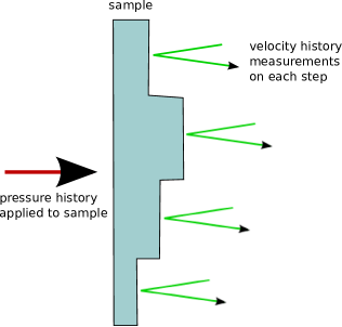
Figure 1: Schematic of ramp wave EOS experiment.

In the iterative analysis used previously Rothman2006 , an estimate of the isentrope $\tilde{p}_{0}(\rho)$ is used to correct the apparent characteristic speed $c^{\prime}(u_{p})$ and thus deduce a modified estimate of the isentrope $\tilde{p}_{1}(\rho)$, repeating until $\tilde{p}_{i}(\rho)$ converges. This is in effect a multivariate non-linear fitting process, which can be computationally intensive if $\tilde{p}_{i}(\rho)$ is slow to converge, can potentially fail by locating a local minimum or can potentially yield solutions which depend on the initial guess $\tilde{p}_{0}(\rho)$, and which is potentially prone to numerical instabilities when the solutions $\tilde{p}_{i}(\rho)$ oscillate around the actual isentrope with increasing amplitude.

As we show next, it is not necessary to assume the solution and iteratively improve it, as all the information is present for a deterministic solution.

III Ramp characteristics at an impedance mismatch

Consider a ramp load applied to one side of a sample of some thickness. At each pressure, the load propagates through the sample as a characteristic of some speed $c$. As the characteristic approaches the opposite side of the sample, it is perturbed by interactions with the reflection of preceding characteristics from the free surface, releasing the pressure gradually to zero at the surface (Fig. 2). When calculating intersections between the characteristics, it is easier to work in the Lagrangian frame, where distances are expressed in terms of the original position of each element of matter within the sample (Fig. 3). The front and back surfaces are then constant in time, and wave speeds are scaled by the compression $\rho/\rho_{0}$.

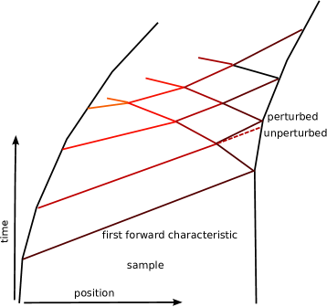
Figure 2: Interaction between successive reflected characteristics in the laboratory frame.

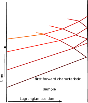
Figure 3: Interaction between successive reflected characteristics in the Lagrangian frame.

At the interface, any given characteristic has been affected by all previous (lower-pressure) characteristics, but not by any subsequent (higher pressure) ones. The effect can be corrected for recursively. Consider the appearance of the characteristic $\chi_{1}$ resulting in the first significant change in interface velocity at some step of thickness $x$ (Fig. 2). This characteristic is unaffected by previous characteristics, so its speed $c_{1}$ can be determined trivially by the difference in arrival time at steps of different height.

The next characteristic $\chi_{2}$ appears at some later time $t_{2}$. However, its propagation to the interface has been perturbed by the reflection of $\chi_{1}$, which travels backward at $-c_{1}$. As the speed of this reflected wave is known, the location at which it must have interacted with the unperturbed $\chi_{2}$ can be calculated:

$$t_{2}^{\prime} = \frac{x_{1}-x_{2}}{2c_{1}}+\frac{t_{1}+t_{2}}{2}$$ (4)

$$x_{2}^{\prime} = x_{2}-c_{1}(t_{2}^{\prime}-t_{2})$$ (5)

This correction can be made for each step, and the corresponding correction can be made for all subsequent characteristics.

Once a characteristic has been corrected for all preceding characteristics, its Lagrangian wave speed (here taken to mean with respect to uncompressed material) can be calculated from the corrected position-time data for two or more steps: $c_{i}=\Delta x_{i}^{\prime}/\Delta t_{i}^{\prime}$. The step height only enters as a difference, so absolute step heights are irrelevant so long as the relative heights are known.

In previous studies of the nature of ramp wave analysis, there was some discussion of the inherent nature of the problem Hinch2010 ; Ockendon2010 . According to our analysis, the determination of an isentrope from surface velocities is inherently deterministic. It is an inverse problem as normally stated, but is well-posed and invertible. A similar approach was postulated in connection with the analysis of ramp wave data using the hodograph transform Ockendon2010 , although as a brief aside, and does not appear to have been developed further.

Although our recursive but deterministic algorithm seems potentially advantageous for speed and to remove the need to guess an approximate isentrope, there is the potential for poor practical performance such as sensitivity to noise. We investigated the performance of the algorithm on simulated experimental data, for which the isentrope could be calculated independently, as described in Section V below.

IV Calculation of compression and normal stress

For a free surface, and ignoring irreversible effects such as plastic flow, the particle speed $u_{p}$ corresponding to a given interface speed $u$ is $u/2$. The mass density then changes with particle speed as

$$\frac{\partial\rho}{\partial u_{p}}=\frac{\rho}{c_{e}}.$$ (6)

The mass density can be integrated implicitly through the characteristics, which is generally more accurate than a simple finite difference update:

$$\rho_{i+1}=\rho_{i}\frac{1+\Delta u_{p}/2\bar{c}_{e}}{1-\Delta u_{p}/2\bar{c}_{e}}$$ (7)

where $\Delta u_{p}$ is the difference in inferred particle velocity between characteristics $i$ and $i+1$, and $\bar{c}_{e}$ is the average longitudinal wave speed.

The corresponding rate of change of pressure through the characteristics is

$$\frac{\partial p}{\partial u_{p}}=\rho c_{e}$$ (8)

which can be integrated numerically as

$$p_{i+1}=p_{i}+\Delta u_{p}\bar{\rho}\bar{c}_{e}.$$ (9)

This finite difference analysis assumes that the sound speed is constant between the points at which the $i$th forward characteristic intersects the $j$th backward characteristic, i.e.

$$c_{i,i-1}=c_{i+1,i}.$$ (10)

Considering the sequence of states induced by the interacting characteristics in pressure-particle speed space, the speeds are equal if characteristics are inferred from surface velocities interpolated at uniform intervals (Fig. 4): intersections between $N$ forward and $N$ backward characteristics occur at $N$ pressures, corresponding to the pressures deduced along the isentrope. In contrast, if velocities are analyzed at varying intervals – which occurs naturally in experimental data taken at uniform intervals of time – then the intersections between characteristics occur at intermediate pressures, so interpolation is required in order to perform the recursive analysis (Fig. 5).

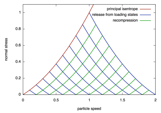
Figure 4: Pressure-particle speed states occurring with free-surface velocity sampled at uniformly-spaced intervals.

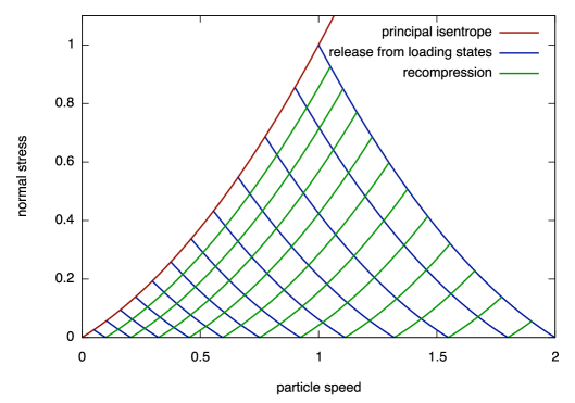
Figure 5: Pressure-particle speed states occurring with free-surface velocity sampled at geometrically-varying intervals.

V Analysis of simulated data

As a test case, we consider the analysis of simulated data for Cu ramp-loaded to 1 TPa. Cu was treated as behaving according to an analytic EOS of the Grüneisen form Steinberg1996 . The peak pressure represents a compression of 2.25, making the loading history prone to forming a shock if not carefully designed. The loading history was chosen to be the ideal shape Swift_idealramp_2008 for an isentrope from this EOS as calculated by numerical integration Swift_genscalar_2008 – the ideal shape being one where all the characteristics cross to form a shock at the same point in the material. This choice does not affect the ramp analysis, but it does eliminate trial and error in choosing step heights suitable for the analysis. The ideal shape was scaled so that the shock formation distance was 200 $\mu$m (Fig. 6), with suitable steps being 140 and 160 $\mu$m. Simulated experimental data were generated from continuum mechanics simulations of the velocity history at the surface of each step (Fig. 7). The simulations were performed using a Lagrangian hydrocode with a second-order predictor-corrector numerical scheme using artificial viscosity to stabilize the flow against unphysical oscillations Benson1992 ; LAGJ . Simulations were performed with spatial resolutions of 1 to 0.1 $\mu$m. Gaussian noise was added to the data in time or velocity.

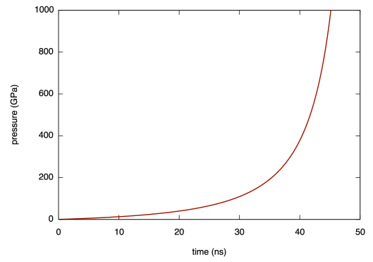
Figure 6: Loading history applied to the Cu to generate simulated data.

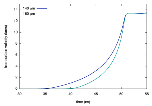
Figure 7: Simulated free-surface velocity histories for steps of different thickness, showing steepening of ramp wave.

The recursive analysis method was implemented as a Java program, and applied to the simulated data, with and without noise. Without noise, the algorithm reproduced the $p(\rho)$ isentrope as calculated directly by integration of the EOS to within 0.5% of the pressure at any given mass density. The discrepancy reduced when the simulated data were generated with finer spatial resolution or sampled with finer temporal resolution, implying that the inaccuracy was dominated by the precision of the hydrocode simulations rather than the analysis method. With noise, the analysis algorithm experienced numerical difficulties if any tabulated $u(t)$ was non-monotonic, which is a trivial filtering constraint. Once filtered, the expected isentrope was recovered to an accuracy commensurate with the noise level. (Fig. 8.)

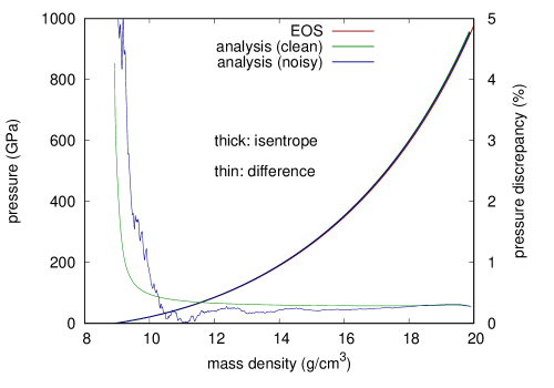
Figure 8: Isentrope obtained by direct integration and by recursive characteristics analysis. (The analysis of data with noise added lies between the isentrope integrated directly from the EOS and the analysis of clean data.)

We did not conduct a rigorous comparison of the computational speed of the recursive algorithm with the iterative algorithm, partly because the latter exhibited difficulties converging to the degree and with the robustness of the former – we found cases where the iterative algorithm failed to converge to a solution, whereas the recursive algorithm continued to reproduce the correct solution. For a typical experimental dataset, with the time sampled at a few hundred values of velocity, the iterative algorithm typically took a few minutes to converge to a solution. The recursive algorithm took around 10 ms, i.e. around $3\times 10^{4}$ faster. (The execution time was dominated by the $\sim$1 s taken to read the ASCII dataset.) For a high resolution dataset, with several thousand points from each step, the increase in speed was approximately $2\times 10^{5}$. Efficiency of this order are useful to make it practicable to embed the ramp analysis within another process, such as iteration over parameters in an additional model such as time-dependence, or uncertainty analysis by Monte-Carlo perturbation of parameters or experimental data. High-throughput analysis also makes it possible to reduce ramp data on times commensurate with the rate of data acquisition on high repetition-rate (multi-Hertz, or faster) experimental platforms.

VI Conclusions

We have developed a non-iterative algorithm – deterministic, and based on recursion over characteristics – for analyzing ramp-loading data, which gives the same results as the iterative algorithm generally used. No numerical problems were found in processing data with noise, though the data had to be filtered to be monotonic.

Comparing with simulated data representative of real experiments, the recursive algorithm was several orders of magnitude faster than the iterative algorithm, and performed more stably, giving a solution in cases where the iterative algorithm failed to converge. Unlike an iterative solution, the recursive algorithm does not require an estimate of the solution to be made as a starting condition, which is undesirable as it may bias the solution.

The deduction of a stress-density relation for a material from surface velocity measurements is inherently deterministic. It is an inverse problem as usually stated, but appears well-posed and invertible.

VII Acknowledgments

Jon Eggert provided an implementation of the iterative algorithm. Steve Rothman (AWE) drew our attention to the papers by Ockendon and Hinch. Tom Arsenlis, Jim McNaney, and Dennis McNabb provided funding and encouragement via the National Nuclear Security Agency’s Science Campaign. This work was performed under the auspices of the U.S. Department of Energy by Lawrence Livermore National Laboratory under Contract DE-AC52-07NA27344.

References

- (1) C.A. Hall, J.R. Asay, M.D. Knudson, W.A. Stygar, R.B. Spielman, T.D. Pointon, D.B. Reisman, A. Toor, and R.C. Cauble, Rev. Sci. Instrum. 72, 3587 (2001).
- (2) J.F. Barnes, P.J. Blewett, R.G. McQueen, K.A., Meyer, and D. Venable, J. Appl. Phys. 45, 727 (1974).
- (3) L.M. Barker in Shock Waves in Condensed Matter – 1983, pp 217-220 (Elsevier, Amsterdam: Elsevier).
- (4) For example, S.T. Weir, A.C. Mitchell, and W.J. Nellis, Phys. Rev. Lett. 76, 11, pp 1860-1863 (1996).
- (5) J. Edwards, K.T. Lorenz, B.A. Remington, S. Pollaine, J. Colvin, D. Braun, B.F. Lasinski, D. Reisman, J.M. McNaney, J.A. Greenough, R. Wallace, H. Louis, and D. Kalantar, Phys. Rev. Lett. 92, 075002 (2004).
- (6) D.C. Swift and R.P. Johnson, Phys. Rev. E 71, 066401 (2005).
- (7) R.F. Smith, J.H. Eggert, A. Jankowski, P.M. Celliers, M.J. Edwards, Y.M. Gupta, J.R. Asay, and G.W. Collins, Phys. Rev. Lett. 98, 065701 (2007).
- (8) D.K. Bradley, J.H. Eggert, R.F. Smith, S.T. Prisbrey, D.G. Hicks, D.G. Braun, J. Biener, A.V. Hamza, R.E. Rudd, and G.W. Collins, Phys. Rev. Lett. 102, 075503 (2009).
- (9) R.G. Kraus, J.-P. Davis, C.T. Seagle, D.E. Fratanduono, D.C. Swift, J.L. Brown, and J.H. Eggert, Phys. Rev. B 93, 134105 (2016).
- (10) S.D. Rothman and J.R. Maw, J. Phys. IV (Procs), 134, pp. 745–750 (2006).
- (11) E.J. Hinch, J. Eng. Math. 68, 279 (2010).
- (12) H Ockendon, J.R. Ockendon, and J.D. Platt, J. Eng. Math. 68, 269 (2010).
- (13) D.J. Steinberg, Equation of state and strength parameters for selected materials, Lawrence Livermore National Laboratory report UCRL-MA-106439 change 1 (1996).
- (14) D.C. Swift, R.G. Kraus, E.N. Loomis, D.G. Hicks, J.M. McNaney, and R.P. Johnson, Phys. Rev. E 78, 066115 (2008).
- (15) D.C. Swift, J. Appl. Phys. 104, 7, 073536 (2008).
- (16) D. Benson, Computer Methods in Appl. Mechanics and Eng. 99, 235 (1992).
- (17) Manual for LAGJ hydrocode V1.1 (Wessex Scientific and Technical Services, Perth, 2015).