On the sensitivity of present direct detection experiments to WIMP–quark and WIMP–gluon effective interactions: a systematic assessment and new model–independent approaches.

Abstract

Assuming for Weakly Interacting Massive Particles (WIMPs) a Maxwellian velocity distribution in the Galaxy we provide an assessment of the sensitivity of existing Dark Matter (DM) direct detection (DD) experiments to operators up to dimension 7 of the relativistic effective field theory describing dark matter interactions with quarks and gluons . In particular we focus on a systematic approach, including an extensive set of experiments and large number of couplings, both exceeding for completeness similar analyses in the literature. The relativistic effective theory requires to fix one coupling for each quark flavor, so in principle for each different combination the bounds should be recalculated starting from direct detection experimental data. To address this problem we propose an approximate model–independent procedure that allows to directly calculate the bounds for any combination of couplings in terms of model–independent limits on the Wilson coefficients of the non–relativistic theory expressed in terms of the WIMP mass and of the neutron–to–proton coupling ratio $c^{n}/c^{p}$. We test the result of the approximate procedure against that of a full calculation, and discuss its possible pitfalls and limitations. We also provide a simple interpolating interface in Python that allows to apply our method quantitatively.

1 Introduction

One of the most popular scenarios for the Dark Matter (DM) which is believed to contribute to up to 27% of the total mass density of the Universe [2] and to more than 90% of the halo of our Galaxy is provided by Weakly Interacting Massive Particles (WIMPs) with a mass in the GeV-TeV range and weak–type interactions with ordinary matter. Such small but non–vanishing interactions can drive WIMP scattering events off nuclear targets, and the measurement of the ensuing nuclear recoils in low–background detectors (direct detection, DD) represents the most straightforward way to detect them. Indeed, a large worldwide effort is currently under way to observe WIMP-nuclear scatterings, but, with the exception of the DAMA collaboration [3, 4, 5, 6] that has been observing for a long time an excess compatible to the annual modulation of a DM signal, many other experiments using different nuclear targets and various background–subtraction techniques [7, 8, 9, 10, 11, 12, 13, 14, 15, 16, 17, 18, 19] have failed to observe any WIMP signal so far.

The calculation of DD expected rates is affected by large uncertainties, of both astrophysical and particle–physics nature. For instance, most of the explicit ultraviolet completions of the Standard Model that stabilize the Higgs vacuum contain WIMP exotic states that are viable DM candidates and for which detailed predictions for WIMP–nuclear scattering can be worked out, leading in most cases to either a Spin Independent (SI) cross section proportional to the square of the target mass number, or to a Spin–Dependent (SD) cross section proportional to the product of the WIMP and the nucleon spins. Crucially, this allows to determine how the WIMP interacts with different targets, and to compare in this way the sensitivity of different detectors to a given WIMP candidate, with the goal of choosing the most effective detection strategy. However, the non–observation of new physics at the Large Hadron Collider (LHC) has prompted the need to go beyond such top–down approach and to use either “effective” or “simplified” models to analyze the data [20], implying a much larger range of possible scaling laws of the WIMP–nucleon cross section on different targets. Moreover, the expected WIMP–induced scattering spectrum depends on a convolution on the velocity distribution $f(\vec{v})$ of the incoming WIMPs, usually described by a thermalized non–relativistic gas described by a Maxwellian distribution whose root–mean–square velocity $v_{rms}\simeq$ 270 km/s is determined from the galactic rotational velocity by assuming equilibrium between gravitational attraction and WIMP pressure. Indeed, such model, usually referred to as Isothermal Sphere, is confirmed by numerical simulations [21], although the detailed merger history of the Milky Way is not known, allowing for the possibility of the presence of sizable non–thermal components for which the density, direction and speed of WIMPs are hard to predict [22].

As far as the latter issue is concerned, for definiteness, in the following we will adopt for the velocity distribution $f(\vec{v})$ of the incoming WIMPs a standard thermalized non–relativistic gas described by a Maxwellian distribution.

On the other hand, in the present paper we wish to focus on the former issue of the scaling law in direct detection, and in particular on how to compare the sensitivities of different experimental set–ups on WIMP–quark and WIMP–gluon effective interactions by making use of model–independent bounds obtained independently at a lower scale on WIMP–nucleon non–relativistic operators. In particular, since the DD process is non–relativistic (NR) it has been understood some time ago [23, 24] that the most general interaction besides the SI and the SD cross sections can be parameterized with an effective Hamiltonian that complies with Galilean symmetry, containing at most 15 terms in the case of a spin–1/2 particle:

$${\bf\mathcal{H}}({\bf{r}}) = \sum_{\tau=0,1}\sum_{j=1}^{15}c_{j}^{\tau}\mathcal{O}_{j}({\bf{r}})\,t^{\tau},$$ (1)

where the $\mathcal{O}_{j}$ operators are listed in [24] and $t^{0}=1$, $t^{1}=\tau_{3}$ denote the $2\times 2$ identity and third Pauli matrix in isospin space, respectively, and the isoscalar and isovector coupling constants $c^{0}_{j}$ and $c^{1}_{j}$, are related to those to protons and neutrons $c^{p}_{j}$ and $c^{n}_{j}$ by $c^{p}_{j}=c^{0}_{j}+c^{1}_{j}$ and $c^{n}_{j}=c^{0}_{j}-c^{1}_{j}$.

Indeed, the NR couplings $c_{j}^{\tau}$ represent the building blocks of the low–energy limit of any ultraviolet theory, so that an understanding of the behaviour of such couplings is crucial for the interpretation of more general scenarios. As a consequence, the NR effective theory (NREFT) of Eq. (1) has been extensively used in the literature to analyze direct detection data [25, 26, 27, 28, 29, 30, 31, 32, 33, 34, 35, 36, 37, 38, 39].

In light of this, in Ref. [40] we provided an assessment of the overall present and future sensitivity of an extensive list of both present and future WIMP direct detection experiments assuming systematically dominance of one of the possible terms of the NR effective Hamiltonian in the calculation of the WIMP–nucleon cross section. In particular, compared to previous analyses adopting the same approach, in Ref. [40] the bounds on the NREFT are presented in a novel model–independent way: for each of the couplings of Eq. (1) a contour plot of the most stringent 90% C.L. bound on the WIMP–nucleon cross section among a comprehensive set of 14 existing experiments is provided as a function the WIMP mass $m_{\chi}$ and of the ratio of the WIMP–neutron and WIMP–proton couplings $c^{n}/c^{p}$ (along with a color code showing the experiment providing it). This approach allows to make the best constraints on the WIMP–proton cross section available in a model–independent way (in A a simple code is introduced that allows to interpolate the $m_{\chi}$–$c^{n}/c^{p}$ planes of Ref. [40] to get the corresponding numerical values) so that, with the exception of cancellations among different NR operators, such bounds can be directly used to get constraints for a given relativistic effective DM scenario when taking its non–relativistic limit, without the need to go through the calculation of the experimental bound starting from the data and to apply the standard machinery used in [40]. The latter includes more refined treatments beside a simple comparison between theoretical predictions and upper bounds, such as background subtraction or the optimal-interval method [41], and may not be trivial for model builders, who have only access from experimental papers to the bounds on the standard isoscalar spin–independent or WIMP–proton/WIMP–neutron spin–dependent cross sections.

However, in spite of its generality, such approach presents some drawbacks: in particular, the interference of different NR operators and especially the sensitivity of such effect to the running of the couplings from the energy scale of the ultraviolet theory to the nucleon scale [42, 43, 44] are difficult to include in a model–independent way, as well as a possible momentum dependence of the Wilson coefficients of the NR theory. In particular, the latter can arise in the case of a long–range interaction such as for electric–dipole or magnetic–dipole DM [45, 46]. Moreover an additional momentum dependence arises when one needs to include the light-meson poles in the case the DM couples to the axial quark current [47, 48].

For the reasons listed above, the use of the limits on the NR couplings of Ref. [40] to calculate the bounds for an effective relativistic model defined at a much larger scale needs to be tested. This is the first main goal of the present paper, where we wish to use the results of Ref. [40] to calculate the bounds on a specific example of relativistic effective theory, and compare the outcome to the full calculation. In particular, we will assess the sensitivity of present DD experiments to a set of operators up to dimension 7 describing dark matter interactions with quarks $q$ and gluons

$${\cal L}_{\chi}=\sum_{q}\sum_{a,d}{\cal C}_{a,q}^{(d)}{\cal Q}_{a,q}^{(d)}+\sum_{b,d}{\cal C}_{b}^{(d)}{\cal Q}_{b}^{(d)},$$ (2)

where the ${\cal C}_{a,q}^{(d)}$, ${\cal C}_{b}^{(d)}$ are dimensional Wilson coefficients. The sums run over the dimensions of the operators, $d=5,6,7$ and the operator labels, $a$ and $b$. If not specified otherwise, we conventionally fix the Wilson parameters at the Electroweak (EW) scale, that we identify with the $Z$ boson mass. The operators ${\cal Q}_{a,q}^{(d)}$, ${\cal Q}_{b}^{(d)}$ that we will analyze are listed in Eqs.(3,4,5), and are the same analyzed in [49]. Analyses on similar sets of relativistic effective operators can also be found in [50, 51, 52, 44].

In particular, once, for each of the relativistic models we consider, the NR Wilson coefficients $c_{j}^{\tau}$ at the nucleon scale are obtained from the ${\cal C}_{a,q}^{(d)}$’s or ${\cal C}_{b}^{(d)}$’s, the expected DD rates only depend on the non–relativistic response functions [53, 54]. In our analysis we will follow closely Ref. [40], so that we address the reader to that paper for the formulas that we use to calculate the expected rates for WIMP–nucleus scattering.

In Ref. [40] we found that 9 experiments out of a total of 14 present Dark Matter searches can provide the most stringent bound on some of the effective couplings for a given choice of $(m_{\chi},c^{n}/c^{p})$. We include the same experiments in the present analysis: XENON1T [7], CDMSlite [10], SuperCDMS [11], PICASSO [13], PICO–60 (using a $CF_{3}I$ target  [14] and a $C_{3}F_{8}$ one [15]), CRESST-II [16, 55], DAMA (average count rate [56]), DarkSide–50 [19]. The details of how each experimental limit has been obtained can be found in the Appendix A of Ref. [40] with the exception of the PICO–60 result with a $C_{3}F_{8}$ target of Ref. [57] that was recently updated with its final result [15]. In particular, in [15] an additional exposure of 1404 kg days at threshold 2.45 keVnr was included in the analysis, lower than that of Ref. [57] where an exposure of 1167 kg days with threshold 3.3 keVnr was used. So, compared to Ref. [40], for PICO–60 we have added the additional run at 2.45 keVnr and updated the efficiency of both runs using the result from Fig.3 of [15]. We stress that in the literature only the bounds from a few experiments (typically XENON1T and PICO–60) are discussed, and only for a few of the effective models of Eqs.(3,4,5) [51, 42, 43, 49, 58, 38, 39, 59]. So the second main goal of the present paper is to focus on a systematic approach, including a number of experiments and of effective couplings that both exceed for completeness previous analyses.

The approach of the present analysis is complementary to that of Ref. [40], but itself not devoid from drawbacks. In particular, the matching of the Wilson coefficients ${\cal C}_{a,q}^{(d)}$’s of the WIMP–quark relativistic interaction into the $c_{j}^{\tau}$’s of the NR WIMP–nucleon Hamiltonian is highly degenerate, since, in principle, the relativistic effective theory requires to fix one coupling for each quark flavor $q$, while the NR theory contains only protons and neutrons. In other words, some assumptions must be made on how the ${\cal C}_{a,q}^{(d)}$’s scale with the flavor $q$. A frequent approach in the literature is to parameterize the theory in terms of a single coupling ${\cal C}_{a,q}^{(d)}$ common to all quarks  [60, 61], and in our analysis we will do the same. However it is worth pointing out that this assumption would not be applicable to the case of the supersymmetric neutralino, for which, for instance, ${\cal C}_{4,q}^{(6)}$ scales as the $Z$–boson coupling in the case of a Higgsino, or ${\cal C}_{5,q}^{(7)}$ depends on the mass and the weak isospin of the quark for a Gaugino–Higgsino mixing. This has important phenomenological consequences: for instance, the ratio of the two vacuum expectation values in supersymmetry, traditionally parameterized as $\tan\beta$, selects through the Yukawa couplings whether the neutralino couples preferentially to up–type or down–type quarks through Higgs exchange, and it is well known in the literature that large and low $\tan\beta$ values imply very different phenomenological scenarios. Indeed, in the case of a generic scaling of the WIMP–quark couplings the only possible way to obtain a consistent limit without reanalyzing the experimental data is to calculate the ratio $c^{n}/c^{p}$ from the ${\cal C}_{a,q}^{(d)}$’s and directly use the NR bounds of [40]. The limit obtained in this way is only valid if one NR coupling dominates the predicted rate and there are no cancellations among the contributions of different NR couplings. So a specific goal of our analysis is also to assess the validity of such a procedure and to discuss the impact of such cancellations in the different relativistic models we consider.

The paper is organized as follows. In Section 2 we list the relativistic Effective Field Theory (EFT) terms that we consider in our analysis and we summarize how we calculate the NR Wilson coefficients starting from each of them; Section 3 is devoted to our quantitative analysis, where we will provide updated exclusion plots for each relativistic model assuming a common coupling ${\cal C}_{a,q}^{(d)}$ for all quarks; in Section 4 we discuss the impact of interferences among different NR couplings, showing that in most cases only one non–relativistic operator dominates the expected rate and the bounds. We will provide our conclusions in Section 5. Finally, in A we provide a simple interpolation code written in Python that, based on the conclusions of Section 4, allows to reproduce most of the results of Section 3 and to generalize them to other choices of the ${\cal C}_{a,q}^{(d)}$ couplings assuming that one non–relativistic operator dominates the expected rate.

2 Relativistic effective models

In this Section we outline the procedure that we follow to obtained the numerical results of Section 3. We use the code DirectDM [49, 48] to calculate the nonperturbative matching of the effective field theory describing dark matter interactions with quarks and gluons at the EW scale to the effective theory of nonrelativistic dark matter interacting with nonrelativistic nucleons (alternative analyses based on chiral effective field theory can be found for instance in [62, 63, 64, 65]). For this reason we follow closely the notation of Ref.[49, 66] and consider the same relativistic operators.

In particular, we consider the two dimension-five operators:

$${\cal Q}_{1}^{(5)}=\frac{e}{8\pi^{2}}(\bar{\chi}\sigma^{\mu\nu}\chi)F_{\mu\nu}\,,\qquad{\cal Q}_{2}^{(5)}=\frac{e}{8\pi^{2}}(\bar{\chi}\sigma^{\mu\nu}i\gamma_{5}\chi)F_{\mu\nu}\,,$$ (3)

where $F_{\mu\nu}$ is the electromagnetic field strength tensor and $\chi$ is the DM field, assumed here to be a Dirac particle. Such operators correspond, respectively, to magnetic–dipole and electric–dipole DM and imply a long–range interaction [67] . The dimension-six operators are

$${\cal Q}_{1,q}^{(6)} = (\bar{\chi}\gamma_{\mu}\chi)(\bar{q}\gamma^{\mu}q)\,,{\cal Q}_{2,q}^{(6)}=(\bar{\chi}\gamma_{\mu}\gamma_{5}\chi)(\bar{q}\gamma^{\mu}q)\,,$$

$${\cal Q}_{3,q}^{(6)} = (\bar{\chi}\gamma_{\mu}\chi)(\bar{q}\gamma^{\mu}\gamma_{5}q)\,,{\cal Q}_{4,q}^{(6)}=(\bar{\chi}\gamma_{\mu}\gamma_{5}\chi)(\bar{q}\gamma^{\mu}\gamma_{5}q)\,,$$ (4)

and we also include the following dimension-seven operators: namely:

$${\cal Q}_{1}^{(7)} = \frac{\alpha_{s}}{12\pi}(\bar{\chi}\chi)G^{a\mu\nu}G_{\mu\nu}^{a}\,,{\cal Q}_{2}^{(7)}=\frac{\alpha_{s}}{12\pi}(\bar{\chi}i\gamma_{5}\chi)G^{a\mu\nu}G_{\mu\nu}^{a}\,,$$

$${\cal Q}_{3}^{(7)} = \frac{\alpha_{s}}{8\pi}(\bar{\chi}\chi)G^{a\mu\nu}\widetilde{G}_{\mu\nu}^{a}\,,{\cal Q}_{4}^{(7)}=\frac{\alpha_{s}}{8\pi}(\bar{\chi}i\gamma_{5}\chi)G^{a\mu\nu}\widetilde{G}_{\mu\nu}^{a}\,,$$

$${\cal Q}_{5,q}^{(7)} = m_{q}(\bar{\chi}\chi)(\bar{q}q)\,,{\cal Q}_{6,q}^{(7)}=m_{q}(\bar{\chi}i\gamma_{5}\chi)(\bar{q}q)\,,$$

$${\cal Q}_{7,q}^{(7)} = m_{q}(\bar{\chi}\chi)(\bar{q}i\gamma_{5}q)\,,{\cal Q}_{8,q}^{(7)}=m_{q}(\bar{\chi}i\gamma_{5}\chi)(\bar{q}i\gamma_{5}q)\,,$$

$${\cal Q}_{9,q}^{(7)} = m_{q}(\bar{\chi}\sigma^{\mu\nu}\chi)(\bar{q}\sigma_{\mu\nu}q)\,,{\cal Q}_{10,q}^{(7)}=m_{q}(\bar{\chi}i\sigma^{\mu\nu}\gamma_{5}\chi)(\bar{q}\sigma_{\mu\nu}q)\,.$$ (5)

In the equations above $q=u,d,s$ denote the light quarks, $G_{\mu\nu}^{a}$ is the QCD field strength tensor, while $\widetilde{G}_{\mu\nu}=\frac{1}{2}\varepsilon_{\mu\nu\rho\sigma}G^{\rho\sigma}$ is its dual, and $a=1,\dots,8$ are the adjoint color indices. In the following we will also assume that all the operators listed in Eqs.(3)–(5) conserve flavor.

A potentially sizeable mixing effect among the vector and axial–vector currents of Eq.(4) is known to be induced by the running of the couplings above the EW scale  [42, 43]. In particular, this may induce a quark vector coupling at the low scale relevant for DD even if the effective theory contains only an axial coupling at the high scale, changing dramatically the DD cross section scaling with the nuclear target and the ensuing DD constrains. For this reason, in the case of the operators of Eq. (4) with a vector–axial quark current, besides the results valid for a given effective operator at the EW scale we also show the corresponding ones when the same operator is defined at the scale $\mu_{scale}$=2 TeV, using the code runDM [69] to evaluate the running from $\mu_{scale}$ to $m_{Z}$=91.1875 GeV. In order to do so we assume that the axial–vector coupling is the same for all quarks at the high scale . We then use the output of runDM as an input for DirectDM to perform the remaining running from $m_{Z}$ to the nucleon scale, where the hadronization of the operators ${\cal Q}_{a,q}^{(d)}$ in eqs. (3,4,5) leads at leading order in the chiral expansion only to single-nucleon (N=p,n) currents, i.e., schematically:

$$<N|\bar{q}\Gamma q|N> = \sum_{\Gamma^{\prime}}\Omega_{N}^{\Gamma^{\prime}}\bar{\Psi}_{N}\Gamma^{\prime}\Psi_{N},$$

$$<N|G^{a\mu\nu}G_{a,\mu\nu}|N> = \Omega_{N}^{\prime}\bar{\Psi}_{N}\Psi_{N},$$

$$<N|G^{a\mu\nu}\tilde{G}_{a,\mu\nu}|N> = \Omega_{N}^{\prime\prime}\bar{\Psi}_{N}\gamma_{5}\Psi_{N},$$ (6)

with $\Gamma$, $\Gamma^{\prime}=1,\gamma^{\mu},\gamma^{\mu}\gamma_{5},\gamma_{5},\sigma^{\mu\nu}$ and $\Psi_{N}$ the nucleon field. Also for the quantities $\Omega$, $\Omega^{\prime}$ and $\Omega^{\prime\prime}$ (which in general can depend on external momenta) we rely on the output of DirectDM (see appendix A of [49]). In particular, the matching of the axial-axial partonic level operator, as well as that of the coupling between the DM particle to the QCD anomaly term leads to pion and eta poles that can be numerically important, and that we include in our analysis. Specifically [49]:

$$\langle N|\bar{q}\gamma^{\mu}\gamma_{5}q|N\rangle = \bar{\Psi}_{N}\Big{[}F_{A}^{q/N}(q^{2})\gamma^{\mu}\gamma_{5}+\frac{1}{2m_{N}}F_{P^{\prime}}^{q/N}(q^{2})\gamma_{5}q^{\mu}\Big{]}\Psi_{N}\,,$$ (7)

$$\langle N|m_{q}\bar{q}i\gamma_{5}q|N\rangle = F_{P}^{q/N}(q^{2})\,\bar{\Psi}_{N}i\gamma_{5}\Psi_{N}\,,$$ (8)

$$\langle N|\frac{\alpha_{s}}{8\pi}G^{a\mu\nu}\tilde{G}^{a}_{\mu\nu}|N\rangle = F_{\tilde{G}}^{N}(q^{2})\,\bar{\Psi}_{N}i\gamma_{5}\Psi_{N}\,,$$ (9)

with:

$$F_{P,P^{\prime}}^{q/N}(q^{2}) = \frac{m_{N}^{2}}{m_{\pi}^{2}-q^{2}}a_{\pi}^{q/N}+\frac{m_{N}^{2}}{m_{\eta}^{2}-q^{2}}a_{\eta}^{q/N}+b^{q/N},$$ (10)

$$F_{\tilde{G}}^{N}(q^{2}) = \frac{q^{2}}{m_{\pi}^{2}-q^{2}}a_{\tilde{G},\pi}^{N}+\frac{q^{2}}{m_{\eta}^{2}-q^{2}}a_{\tilde{G},\eta}^{N}+b_{\tilde{G}}^{N},$$ (11)

where we use DirectDM and runDM when applicable to calculate the coefficients $a$ and $b$ from the high–energy couplings, and $q^{2}$ represents here the squared four–momentum transfer. Finally, taking the non–relativistic limit, we obtain the coefficients $c_{i}^{\tau}$ of the effective Hamiltonian of Eq. (1), which turn out to be proportional to the initial relativistic dimensional coupling ${\cal C}_{a,q}^{(d)}$, and, in general, depend on the WIMP mass $m_{\chi}$ and on the exchanged momentum $q$ (the latter dependence both through the poles of Eqs.(10,11) and because of the photon propagator induced by the dimension–5 magnetic and electric dipole operators of Eq. (3)).

For the details of the expression to calculate the expected rate in a DD experiment we refer, for instance, to Section 2 of [40]. In particular, the differential cross section is proportional to the squared amplitude:

$$\frac{d\sigma_{T}}{dE_{R}}=\frac{2m_{T}}{4\pi v_{T}^{2}}\left[\frac{1}{2j_{\chi}+1}\frac{1}{2j_{T}+1}|\mathcal{M}_{T}|^{2}\right],$$ (12)

with $v_{T}\equiv|\vec{v}_{T}|$ the WIMP speed in the reference frame of the nuclear center of mass, $m_{T}$ the nuclear mass, $j_{T}$, $j_{\chi}$ are the spins of target nucleus and WIMP, and [24]:

$$\frac{1}{2j_{\chi}+1}\frac{1}{2j_{T}+1}|\mathcal{M}_{T}|^{2}=\frac{4\pi}{2j_{T}+1}\sum_{\tau=0,1}\sum_{\tau^{\prime}=0,1}\sum_{k}R_{k}^{\tau\tau^{\prime}}\left[c^{\tau}_{i},c_{j}^{\tau^{\prime}},(v^{\perp}_{T})^{2},\frac{q^{2}}{m_{N}^{2}}\right]W_{Tk}^{\tau\tau^{\prime}}(y).$$ (13)

In the above expression the squared amplitude $|\mathcal{M}_{T}|^{2}$ is summed over initial and final spins, the $R_{k}^{\tau\tau^{\prime}}$’s are WIMP response functions which depend on the couplings $c^{\tau}_{j}$ as well as the transferred momentum $\vec{q}$, while:

$$(v^{\perp}_{T})^{2}=v^{2}_{T}-v_{min}^{2},$$ (14)

and:

$$v_{min}^{2}=\frac{q^{2}}{4\mu_{T}^{2}}=\frac{m_{T}E_{R}}{2\mu_{T}^{2}},$$ (15)

represents the minimal incoming WIMP speed required to impart the nuclear recoil energy $E_{R}$. Moreover, in equation (13) the $W^{\tau\tau^{\prime}}_{Tk}(y)$’s are nuclear response functions and the index $k$ represents different effective nuclear operators, which, under the assumption that the nuclear ground state is an approximate eigenstate of $P$ and $CP$, can be at most eight: following the notation in [23, 24], $k$=$M$, $\Phi^{\prime\prime}$, $\Phi^{\prime\prime}M$, $\tilde{\Phi}^{\prime}$, $\Sigma^{\prime\prime}$, $\Sigma^{\prime}$, $\Delta$, $\Delta\Sigma^{\prime}$. The $W^{\tau\tau^{\prime}}_{Tk}(y)$’s are function of $y\equiv(qb/2)^{2}$, where $b$ is the size of the nucleus. For the target nuclei $T$ used in most direct detection experiments the functions $W^{\tau\tau^{\prime}}_{Tk}(y)$, calculated using nuclear shell models, have been provided in Refs. [24, 70]. Details about the definitions of both the functions $R_{k}^{\tau\tau^{\prime}}$’s and $W^{\tau\tau^{\prime}}_{Tk}(y)$’s can be found in [24]. In particular, using the decomposition:

$$R_{k}^{\tau\tau^{\prime}}=R_{0k}^{\tau\tau^{\prime}}+R_{1k}^{\tau\tau^{\prime}}(v^{\perp}_{T})^{2}=R_{0k}^{\tau\tau^{\prime}}+R_{1k}^{\tau\tau^{\prime}}\left(v_{T}^{2}-v_{min}^{2}\right),$$ (16)

the correspondence between each term of the NR effective interaction in (1) and the $W^{\tau\tau^{\prime}}_{Tk}(y)$ nuclear response functions is summarized in Table 1. Notice that $W_{M}$ corresponds to the standard SI interaction, while $W_{\Sigma^{\prime\prime}}+W_{\Sigma^{\prime}}$ (with $W_{\Sigma^{\prime}}\simeq 2W_{\Sigma^{\prime\prime}}$) to the standard SD one.

coupling	$R^{\tau\tau^{\prime}}_{0k}$	$R^{\tau\tau^{\prime}}_{1k}$	coupling	$R^{\tau\tau^{\prime}}_{0k}$	$R^{\tau\tau^{\prime}}_{1k}$
$1$	$M(q^{0})$	-	$3$	$\Phi^{\prime\prime}(q^{4})$	$\Sigma^{\prime}(q^{2})$
$4$	$\Sigma^{\prime\prime}(q^{0})$,$\Sigma^{\prime}(q^{0})$	-	$5$	$\Delta(q^{4})$	$M(q^{2})$
$6$	$\Sigma^{\prime\prime}(q^{4})$	-	$7$	-	$\Sigma^{\prime}(q^{0})$
$8$	$\Delta(q^{2})$	$M(q^{0})$	$9$	$\Sigma^{\prime}(q^{2})$	-
$10$	$\Sigma^{\prime\prime}(q^{2})$	-	$11$	$M(q^{2})$	-
$12$	$\Phi^{\prime\prime}(q^{2})$,$\tilde{\Phi}^{\prime}(q^{2})$	$\Sigma^{\prime\prime}(q^{0})$,$\Sigma^{\prime}(q^{0})$	$13$	$\tilde{\Phi}^{\prime}(q^{4})$	$\Sigma^{\prime\prime}(q^{2})$
$14$	-	$\Sigma^{\prime}(q^{2})$	$15$	$\Phi^{\prime\prime}(q^{6})$	$\Sigma^{\prime}(q^{4})$

Table 1: Nuclear response functions corresponding to each coupling, for the velocity–independent and the velocity–dependent components parts of the WIMP response function, decomposed as in Eq.(16). In parenthesis is the power of $q$ in the WIMP response function.

Finally, for the WIMP local density we take $\rho_{loc}$=0.3 GeV/cm³ and for the velocity distribution we assume a standard isotropic Maxwellian at rest in the Galactic rest frame boosted to the Lab frame by the velocity of the Sun, $v_{\odot}$=232 km/s, with root–mean–square velocity $v_{rms}$=270 km/s and truncated at the escape velocity $u_{esc}$=550 km/s.

3 Analysis

In this Section for each of the models ${\cal Q}^{(d)}_{a,q}$, ${\cal Q}^{(d)}_{b}$ listed in Eqs. (3–5) we show the present constraints on the correspondent dimensional coupling ${\cal C}^{(d)}_{a,q}$ (assumed to be the same for all flavors) and ${\cal C}^{(d)}_{b}$ from the list of experiments summarized in the Introduction (XENON1T [7], CDMSlite [10], SuperCDMS [11], PICASSO [13], PICO–60 (using a $CF_{3}I$ target  [14] and a $C_{3}F_{8}$ one [15]), CRESST-II [16, 55], DAMA (average count rate) [56], DarkSide–50 [19]) in terms of lower bounds on the effective scale $\tilde{\Lambda}$ defined through:

$${\cal C}^{(d)}_{a,q},{\cal C}^{(d)}_{b}\equiv\frac{1}{\tilde{\Lambda}^{d-4}}.$$ (17)

As a default choice in all cases we fix ${\cal C}^{(d)}_{a,q}$, ${\cal C}^{(d)}_{b}$ at the EW scale, identified as the $Z$–boson mass, $\mu_{scale}$= $m_{Z}$. Only for the 6–dimensional interaction terms ${\cal Q}^{(6)}_{3,q}$ and ${\cal Q}^{(6)}_{4,q}$ we also show in Fig. 4 the result obtained when the ${\cal C}^{(d)}_{a,q}$ coupling is fixed at the scale $\mu_{scale}$= 2 TeV and run down to the EW scale using runDM and assuming that the axial–vector coupling is the same for all quarks at the high scale. One can notice that in the case of ${\cal Q}^{(6)}_{3,q}$ passing from $\mu_{scale}$=$m_{Z}$ to $\mu_{scale}$=2 TeV the experimental bound is strengthened by more than two orders of magnitude. This is a well–known effect [42, 43] due to the mixing between ${\cal Q}^{(6)}_{3,q}$ and ${\cal Q}^{(6)}_{1,q}$ induced by the running from 2 TeV to $m_{Z}$. In particular, without such mixing ${\cal Q}^{(6)}_{3,q}$ gives rise to two NR operators that have both a spin–dependent type scaling with the target, ${\cal O}_{9}$ and ${\cal O}_{7}$, the latter also velocity suppressed [40], while the mixing due to running induces a ${\cal Q}^{(6)}_{1,q}$ component leading to the SI ${\cal O}_{1}$ operator (see Tables 1 and 2) that overwhelms the other contributions in spite of the loop–suppressed Wilson coefficient. Such effect is also present for the ${\cal Q}^{(6)}_{4,q}$ operator due to the mixing with ${\cal Q}^{(6)}_{2,q}$, although in this case the effect on the exclusion plot is less sizable. It is worth pointing out here that the mixing between vector and vector–axial currents is driven by the coupling between the DM particle and the quarks of the third family, so it is not present if the latter is assumed to vanish. In such case the results of Fig. 4 would coincide to those of Fig. 3.

In all the plots the data are analyzed in the same way of the experimental collaborations to obtain lower bounds on the effective scale $\tilde{\Lambda}$ defined in Eq. (17) as a function of the WIMP mass $m_{\chi}$ assuming a single flavor–independent coupling ${\cal C}_{a,q}^{(d)}$ common to all quarks. In particular, for all experiments with the exception of SuperCDMS and DarkSide–50 we compare the expected rate to the 90% C.L. upper bound on the count rate in each energy bin assuming zero background. Namely, for XENON1T we have assumed 7 WIMP candidate events in the range of 3 PE $\leq S_{1}\leq$ 70 PE, as shown in Fig. 3 of Ref. [7] for the primary scintillation signal S1 (directly in Photo Electrons, PE), with an exposure of 278.8 days, fiducial volume of 1.3 ton and the efficiency taken from Fig. 1 of Ref. [7]. In the analysis of DarkSide–50, we subtract the estimated background by fitting the data at fixed $m_{\chi}$ to the sum $S_{i}(\tilde{\Lambda})+\lambda b_{i}$ in terms of the two free parameters $\tilde{\Lambda}$ and $\lambda$ [40], with $S_{i}$ the expected WIMP signal in each energy bin $i$ and $b_{i}$ taken from Fig. 3 of [19] using the exposure of 6786.0 kg days. This latter procedure is particularly effective when the spectral shapes of the signal and of the background are different. For DarkSide–50 the estimated spectrum of the background is rising with the recoil energy, so it yields a weaker constraint for interactions types with an explicit momentum dependence that lead to a signal rising with energy in a way similar to the background. This loss of constraining power is the reason of the peculiar shapes of some of the exclusion plots for DarkSide–50 in Figs. 1–9. The latest SuperCDMS analysis [11] observed 1 event between 4 and 100 keVnr with an exposure of 1690 kg days. To analyze the observed spectrum we apply the the maximum–gap method [41] with the efficiency taken from Fig. 1 of [11] and the energy resolution $\sigma=\sqrt{0.293^{2}+0.056^{2}E_{ee}/\rm keVee}~{}\rm keVee$ from [71]. In the case of CDMSlite, we consider the energy bin 0.056 keV$<E^{\prime}<$ 1.1 keV with a measured count rate of 1.1$\pm$0.2 [keV kg days]^-1 (Full Run 2 rate, Table II of Ref. [10]). We have taken the efficiency from Fig. 4 of [10] and the energy resolution $\sigma=\sqrt{\sigma_{E}^{2}+BE_{R}+(AE_{R})^{2}}$, with $\sigma_{E}$=9.26 eV, $A$=5.68$\times 10^{-3}$ and $B$=0.64 eV from Section IV.A of [10]. In the case of threshold detectors such as PICO60 and PICASSO, we consider for each threshold an energy bin up to the maximal recoil energy allowed by the escape velocity. For PICASSO we take into account the six energy thresholds ($E_{th}$=1.0, 1.5, 2.7, 6.6,15.7,36.8 keV) analyzed in [13] while for PICO-60 we considered the threshold $E_{th}$=3.3 keV with a total exposure of 1167.0 kg days and no event detected [57]. PICO-60 can also employ a $CF_{3}I$ target and in this case we adopt an energy threshold of 13.6 keV and an exposure of 1335 kg days [14]. For DAMA we consider the upper bound from the average count rate (DAMA0) which has been taken from [56] (rebinned from 0.25-keVee- to 0.5-keVee-width bins). We assume constant quenching factors $q$=0.3 for sodium and $q$=0.09 for iodine, and the energy resolution $\sigma$ = 0.0091 (E_ee/keVee) + 0.448 $\sqrt{E_{ee}/{\rm keVee}}$ in keV. For the CRESST-II experiment, we considered the Lise module analysis from [16] with energy resolution $\sigma$=0.062 keV and detector efficiency from Fig. 4 of [72]. In our analysis, we have selected 15 events for 0.3 keVnr$<E_{R}<$ 0.49 keVnr with an exposure of 52.15 kg days. With the assumptions summarized above we reproduce published results in the case of a standard Spin–Independent interaction. Further details can be found in Appendix A of Ref. [40].

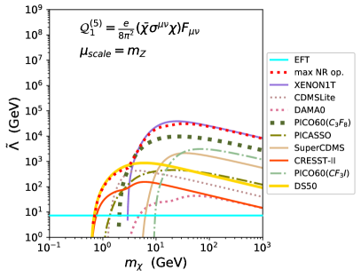
Figure 1: Lower bound on the effective scale $\tilde{\Lambda}$ defined in Eq. (17) for the operators ${\cal Q}^{(5)}_{1,q}$ (left) and ${\cal Q}^{(5)}_{2,q}$ (right). In both cases the dimensional couplings ${\cal C}^{(5)}_{1,q}$ and ${\cal C}^{(5)}_{2,q}$ are fixed at the EW scale $\mu_{scale}$=$m_{Z}$. In the region below the solid cyan line the limits are inconsistent with the validity of the EFT based on the simple criterion introduced in Section 3.

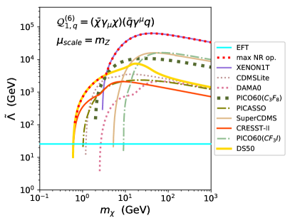
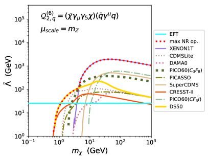
Figure 2: The same as in Fig. 1 for ${\cal Q}^{(6)}_{1,q}$ (left) and ${\cal Q}^{(6)}_{2,q}$ (right).

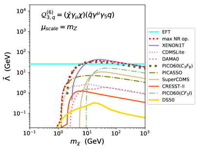
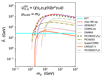
Figure 3: The same as in Fig. 2 for ${\cal Q}^{(6)}_{3,q}$ (left) and ${\cal Q}^{(6)}_{4,q}$ (right).

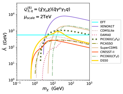
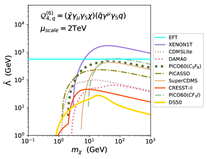
Figure 4: The same as in Fig. 3 for $\mu_{scale}$=2 TeV.

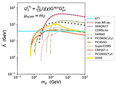
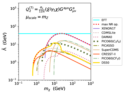
Figure 5: The same as in Fig. 2 for ${\cal Q}^{(7)}_{1}$ (left) and ${\cal Q}^{(7)}_{2}$ (right).

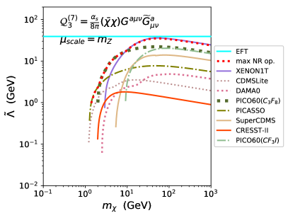
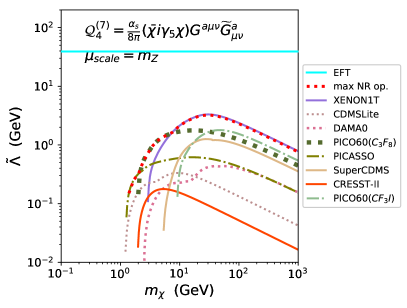
Figure 6: The same as in Fig. 2 for ${\cal Q}^{(7)}_{3}$ (left) and ${\cal Q}^{(7)}_{4}$ (right).

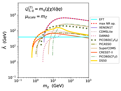
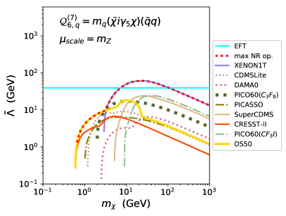
Figure 7: The same as in Fig. 2 for ${\cal Q}^{(7)}_{5}$ (left) and ${\cal Q}^{(7)}_{6}$ (right).

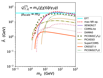
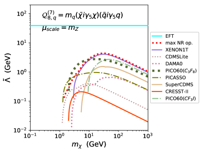
Figure 8: The same as in Fig. 2 for ${\cal Q}^{(7)}_{7}$ (left) and ${\cal Q}^{(7)}_{8}$ (right).

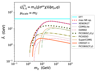
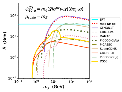
Figure 9: The same as in Fig. 2 for ${\cal Q}^{(7)}_{9}$ (left) and ${\cal Q}^{(7)}_{10}$ (right).

The exclusion plots of Figs. 1–9 can be roughly devided in two classes: in the case of models ${\cal Q}^{(5)}_{1,q}$, ${\cal Q}^{(5)}_{2,q}$, ${\cal Q}^{(6)}_{1,q}$, ${\cal Q}^{(6)}_{2,q}$, ${\cal Q}^{(7)}_{1}$, ${\cal Q}^{(7)}_{2}$, ${\cal Q}^{(7)}_{5,q}$, ${\cal Q}^{(7)}_{6,q}$ and ${\cal Q}^{(7)}_{10,q}$ the most constraining experiments are DarkSide–50 at low WIMP mass and XENON1T at larger $m_{\chi}$. As can be seen by combining Table 2 (that allows to see the correspondence between each ${\cal Q}^{(d)}_{a,q}$, ${\cal Q}^{(d)}_{b}$ term and NR operators) and Table 1 (where the correspondence between each NR operator ${O}_{i}$ and the nuclear response functions $W^{\tau\tau^{\prime}}_{Tk}(y)$’s is shown) one can see that all such interactions take contributions from the $W_{M}$ nuclear response function, leading to a SI scaling of the cross section (possibly combined with explicit dependence from the exchanged momentum $q^{2}$ and from the WIMP incoming speed ). Indeed, due to its very low threshold DarkSide–50 drives the exclusion plot at low mass, but only for interactions that do not require a nuclear spin (its target is ⁴⁰Ar), while at larger masses the SI coupling enhances the sensitivity for scatterings off xenon in XENON1T. The second class of exclusion plots is represented by the models ${\cal Q}^{(6)}_{3,q}$, ${\cal Q}^{(6)}_{4,q}$, ${\cal Q}^{(7)}_{3}$, ${\cal Q}^{(7)}_{4}$, ${\cal Q}^{(7)}_{7,q}$, ${\cal Q}^{(7)}_{8,q}$, and ${\cal Q}^{(7)}_{9,q}$ for which the exclusion plot is driven by PICASSO and PICO60 (and, sometimes, by CDMSLite) at low WIMP mass, and by XENON1T at larger WIMP masses. In such cases, as can again be seen from Tables 2 and 1, the operator $M$ is always missing in the NR limit, while the response functions $\Sigma^{\prime}$ and/or $\Sigma^{\prime\prime}$ are always present, leading to a SD–type scaling of the cross section for which large detectors containing fluorine are competitive with xenon.

Some of the limits shown in Figs. 1–9 may be so weak that they put bounds on values of the $\tilde{\Lambda}$ scale which are inconsistent with the validity of the effective theory. In such case one can simply conclude that the present experimental sensitivity of direct detection experiments is not able to put bounds on the corresponding effective operator. A criterion for the validity of the EFT is to interpret the scale $\tilde{\Lambda}$ in terms of a propagator $g^{2}/M_{*}^{2}$ with $g<\sqrt{4\pi}$ and $M_{*}>\mu_{scale}$, since in our analysis we fixed the boundary conditions of the EFT at the scale $\mu_{scale}$. This is straightforward for dimension–6 operators, while in the case of operators whose effective coupling has dimension different from -2 only matching the EFT with the full theory would allow to draw robust conclusions. In particular, in this case $\tilde{\Lambda}$ can be interpreted in terms of the same propagator times the appropriate power of a typical scale of the problem $\mu_{scale}^{\prime}$, which depends on the ultraviolet completion of the EFT. For instance, in the operator ${\cal Q}_{5,q}^{(7)}$=$m_{q}(\bar{\chi}\chi)(\bar{q}q)$ the quark mass may originate from a Yukawa coupling, so the missing scale is an Electroweak vacuum expectation value in the denominator. To fix an order of magnitude we choose to fix $\mu_{scale}^{\prime}$ = $\mu_{scale}$, so that the bound $\tilde{\Lambda}>\mu_{scale}/(4\pi)^{1/(d-4)}$ can be derived. Such limit is shown as a horizontal solid line in Figs. 1–9. In particular, for models ${\cal Q}^{(7)}_{2}$, ${\cal Q}^{(7)}_{3}$, ${\cal Q}^{(7)}_{4}$, ${\cal Q}^{(7)}_{6}$, ${\cal Q}^{(7)}_{7}$, ${\cal Q}^{(7)}_{8}$ and ${\cal Q}^{(7)}_{9}$ the bound on the $\tilde{\Lambda}$ scale lies above such curve in all the WIMP mass range, implying that the sensitivities of present direct detection experiments to such couplings may not be sufficient to put meaningful bounds. However we stress again that this can only be assessed when a specific ultraviolet completion of the effective theory is assumed.

In A we introduce

RDD_constraints }, a simple
interpolating code written in Python that can reproduce most of the
results of this Section by assuming that one 

R coupling dominates in the low–energy limit of the interactions of Eqs.(3)–(5). In Figs. 1–3 and Figs. 5–9 the output of such code is indicated by “max NR op.” and represented by the red–dashed curve. One can see that, with the exception of models ${\cal Q}_{7,q}^{(7)}$ and ${\cal Q}_{8,q}^{(7)}$, the “max NR op.” matches the lower edge of the excluded region obtained through a full calculation.

4 Interference and momentum effects in the NR theory

No matter which among the relativistic interactions listed in Eqs.(3,4,5) is generated at a higher scale by some beyond–the–standard–model scenario, Dark Matter DD scattering is a low–energy process completely described by the NR effective theory of (Eq. 1). This implies that the limits discussed in the previous Section can be expressed in terms of NR operators only. In particular, in the case of interactions between the DM particle and the quark current, this would have the advantage to present the limits from existing experiments in a way independent from the choice of the ${\cal C}_{a,q}^{(d)}$ couplings for each flavor $q$, since the NR effective theory depends only on WIMP mass and on the ratio between the WIMP–neutron and the WIMP–proton couplings $r\equiv c^{n}/c^{p}$. Indeed, in ref. [40] we obtained updated upper bounds on the effective cross section:

$$\sigma^{\cal N}_{i}=\max(\sigma^{p}_{i},\sigma^{n}_{i}),$$ (18)

with:

$$\sigma^{p,n}_{i}=(c_{i}^{p,n})^{2}\frac{\mu_{\chi{\cal N}}^{2}}{\pi},$$ (19)

($\mu_{\chi{\cal N}}$ is the WIMP–nucleon reduced mass) assuming constant couplings $c_{i}^{p,n}$ and, systematically, dominance of one of the possible NR interaction terms ${\cal O}_{i}$ of Eq. (1), providing for each of them a two–dimensional plot where the contours of the most stringent 90% C.L. upper bounds to $\sigma^{\cal N}_{i}$ were shown as a function of the two parameters $m_{\chi}$ (WIMP mass), and $c^{n}/c^{p}$. One possible drawback of this approach is however that, in general, a given relativistic coupling leads to more than one NR operator. In addition to that, as explained in Section 2, the NR coefficients $c_{i}^{\tau}$ may depend explicitly on the exchanged momentum, leading, in practice, to contributions which are equivalent to including additional NR operators of the type $F_{i}^{\alpha}(q^{2}){\cal O}_{i}$ (where, for each operator ${\cal O}_{i}$ different momentum dependences are possible, as for instance in Eqs.(10,11)). In fact, setting:

$$c_{i}^{\tau}(m_{\chi},q^{2}) \equiv \hat{c}_{i,\alpha}^{\tau}(m_{\chi})F_{i}^{\alpha}(q^{2})\,,$$ (20)

$$R_{k}^{\tau\tau^{\prime}} \equiv c^{\tau}_{i}c^{\tau^{\prime}}_{j}\hat{R}^{\tau\tau^{\prime}}_{k,ij}=\hat{c}^{\tau}_{i,\alpha}\hat{c}^{\tau^{\prime}}_{j,\beta}\hat{R}^{\tau\tau^{\prime}}_{k,ij}F_{i}^{\alpha}(q^{2})F_{j}^{\beta}(q^{2})\,,$$ (21)

the squared amplitude (13) can be rewritten as:

$$\frac{1}{2j_{\chi}+1}\frac{1}{2j_{T}+1}|\mathcal{M}_{T}|^{2} = \frac{4\pi}{2j_{T}+1}\sum_{ij}\sum_{\alpha\beta}\sum_{\tau,\tau^{\prime}}\hat{c}_{i,\alpha}^{\tau}\hat{c}_{j,\beta}^{\tau^{\prime}}\left[\sum_{k}\hat{R}^{\tau\tau^{\prime}}_{k,ij}W^{\tau\tau^{\prime}}_{k}(q^{2})\right]F_{i}^{\alpha}(q^{2})F_{j}^{\beta}(q^{2}),$$

so that the expected rate $R$ can be expressed as a sum over all possible interferences among the contributions from each generalized NR term $F_{i}^{\alpha}(q^{2}){\cal O}_{i}$:

$$R=\sum_{ij}\sum_{\alpha\beta}\sum_{\tau,\tau^{\prime}}\hat{c}_{i,\alpha}^{\tau}\hat{c}_{j,\beta}^{\tau^{\prime}}\langle{\cal O}_{i}{\cal O}_{j}F_{i}^{\alpha}(q^{2})F_{j}^{\beta}(q^{2})\rangle_{\tau\tau^{\prime}}.$$ (22)

In the equation above each term $\langle{\cal O}_{i}{\cal O}_{j}F_{i}^{\alpha}(q^{2})F_{j}^{\beta}(q^{2})\rangle_{\tau\tau^{\prime}}$ simply represents the factor that multiplies $\hat{c}_{i,\alpha}^{\tau}\hat{c}_{j,\beta}^{\tau^{\prime}}$ at fixed $i$, $j$, $\alpha$, $\beta$, $\tau$, $\tau^{\prime}$ in the expected rate. The terms contributing to the sums over $i$, $j$, $\alpha$, $\beta$ for each of the interactions discussed in Section 3 are listed in Table 2.

${\cal Q}_{1}^{(5)}$	$\hat{c}_{1}^{\tau}\hat{c}_{1}^{\tau^{\prime}}\langle{\cal O}_{1}{\cal O}_{1}\rangle_{\tau\tau^{\prime}}+\hat{c}_{5}^{\tau}\hat{c}_{5}^{\tau^{\prime}}\langle{\cal O}_{5}{\cal O}_{5}\frac{1}{q^{4}}\rangle_{\tau\tau^{\prime}}+\hat{c}_{4}^{\tau}\hat{c}_{4}^{\tau^{\prime}}\langle{\cal O}_{4}{\cal O}_{4}\rangle_{\tau\tau^{\prime}}$
	$+\hat{c}_{6}^{\tau}\hat{c}_{6}^{\tau^{\prime}}\langle{\cal O}_{6}{\cal O}_{6}\frac{1}{q^{4}}\rangle_{\tau\tau^{\prime}}+\hat{c}_{4}^{\tau}\hat{c}_{5}^{\tau^{\prime}}\langle{\cal O}_{4}{\cal O}_{5}\frac{1}{q^{2}}\rangle_{\tau\tau^{\prime}}+\hat{c}_{4}^{\tau}\hat{c}_{6}^{\tau^{\prime}}\langle{\cal O}_{4}{\cal O}_{6}\frac{1}{q^{2}}\rangle_{\tau\tau^{\prime}}$
${\cal Q}_{2}^{(5)}$	$\hat{c}_{11}^{\tau}\hat{c}_{11}^{\tau^{\prime}}\langle{\cal O}_{11}{\cal O}_{11}\frac{1}{q^{4}}\rangle_{\tau\tau^{\prime}}$
${\cal Q}_{1}^{(6)}$	$\hat{c}_{1}^{\tau}\hat{c}_{1}^{\tau^{\prime}}\langle{\cal O}_{1}{\cal O}_{1}\rangle_{\tau\tau^{\prime}}$
${\cal Q}_{2}^{(6)}$	$\hat{c}_{8}^{\tau}\hat{c}_{8}^{\tau^{\prime}}\langle{\cal O}_{8}{\cal O}_{8}\rangle_{\tau\tau^{\prime}}+\hat{c}_{9}^{\tau}\hat{c}_{9}^{\tau^{\prime}}\langle{\cal O}_{9}{\cal O}_{9}\rangle_{\tau\tau^{\prime}}+\hat{c}_{8}^{\tau}\hat{c}_{9}^{\tau^{\prime}}\langle{\cal O}_{8}{\cal O}_{9}\rangle_{\tau\tau^{\prime}}$
${\cal Q}_{3}^{(6)}$	$\hat{c}_{7}^{\tau}\hat{c}_{7}^{\tau^{\prime}}\langle{\cal O}_{7}{\cal O}_{7}\rangle_{\tau\tau^{\prime}}+\hat{c}_{9}^{\tau}\hat{c}_{9}^{\tau^{\prime}}\langle{\cal O}_{9}{\cal O}_{9}\rangle_{\tau\tau^{\prime}}$
${\cal Q}_{4}^{(6)}$	$\hat{c}_{4}^{\tau}\hat{c}_{4}^{\tau^{\prime}}\langle{\cal O}_{4}{\cal O}_{4}\rangle_{\tau\tau^{\prime}}+\hat{c}_{6}^{\tau}\hat{c}_{6}^{\tau^{\prime}}\langle{\cal O}_{6}{\cal O}_{6}\rangle_{\tau\tau^{\prime}}$
	$+\hat{c}_{6}^{\tau}\hat{c}_{6}^{\tau^{\prime}}\langle{\cal O}_{6}{\cal O}_{6}\frac{m^{4}_{N}}{(m^{2}_{\pi}-q^{2})^{2}}\rangle_{\tau\tau^{\prime}}+\hat{c}_{6}^{\tau}\hat{c}_{6}^{\tau^{\prime}}\langle{\cal O}_{6}{\cal O}_{6}\frac{m^{4}_{N}}{(m^{2}_{\pi}-q^{2})(m^{2}_{\eta}-q^{2})}\rangle_{\tau\tau^{\prime}}$
	$+\hat{c}_{6}^{\tau}\hat{c}_{6}^{\tau^{\prime}}\langle{\cal O}_{6}{\cal O}_{6}\frac{m^{4}_{N}}{(m^{2}_{\eta}-q^{2})^{2}}\rangle_{\tau\tau^{\prime}}+\hat{c}_{6}^{\tau}\hat{c}_{6}^{\tau^{\prime}}\langle{\cal O}_{6}{\cal O}_{6}\frac{m^{2}_{N}}{(m^{2}_{\pi}-q^{2})}\rangle_{\tau\tau^{\prime}}+\hat{c}_{6}^{\tau}\hat{c}_{6}^{\tau^{\prime}}\langle{\cal O}_{6}{\cal O}_{6}\frac{m^{2}_{N}}{(m^{2}_{\eta}-q^{2})}\rangle_{\tau\tau^{\prime}}$
	$+\hat{c}_{4}^{\tau}\hat{c}_{6}^{\tau^{\prime}}\langle{\cal O}_{4}{\cal O}_{6}\frac{m^{2}_{N}}{(m^{2}_{\pi}-q^{2})}\rangle_{\tau\tau^{\prime}}+\hat{c}_{4}^{\tau}\hat{c}_{6}^{\tau^{\prime}}\langle{\cal O}_{4}{\cal O}_{6}\frac{m^{2}_{N}}{(m^{2}_{\eta}-q^{2})}\rangle_{\tau\tau^{\prime}}+\hat{c}_{4}^{\tau}\hat{c}_{6}^{\tau^{\prime}}\langle{\cal O}_{4}{\cal O}_{6}\rangle_{\tau\tau^{\prime}}$
${\cal Q}_{1}^{(7)}$	$\hat{c}_{1}^{\tau}\hat{c}_{1}^{\tau^{\prime}}\langle{\cal O}_{1}{\cal O}_{1}\rangle_{\tau\tau^{\prime}}$
${\cal Q}_{2}^{(7)}$	$\hat{c}_{11}^{\tau}\hat{c}_{11}^{\tau^{\prime}}\langle{\cal O}_{11}{\cal O}_{11}\rangle_{\tau\tau^{\prime}}$
${\cal Q}_{3}^{(7)}$	$\hat{c}_{10}^{\tau}\hat{c}_{10}^{\tau^{\prime}}\langle{\cal O}_{10}{\cal O}_{10}\rangle_{\tau\tau^{\prime}}+\hat{c}_{10}^{\tau}\hat{c}_{10}^{\tau^{\prime}}\langle{\cal O}_{10}{\cal O}_{10}\frac{q^{4}}{(m^{2}_{\pi}-q^{2})^{2}}\rangle_{\tau\tau^{\prime}}+\hat{c}_{10}^{\tau}\hat{c}_{10}^{\tau^{\prime}}\langle{\cal O}_{10}{\cal O}_{10}\frac{q^{4}}{(m^{2}_{\pi}-q^{2})(m^{2}_{\eta}-q^{2})}\rangle_{\tau\tau^{\prime}}$
	$+\hat{c}_{10}^{\tau}\hat{c}_{10}^{\tau^{\prime}}\langle{\cal O}_{10}{\cal O}_{10}\frac{q^{4}}{(m^{2}_{\eta}-q^{2})^{2}}\rangle_{\tau\tau^{\prime}}+\hat{c}_{10}^{\tau}\hat{c}_{10}^{\tau^{\prime}}\langle{\cal O}_{10}{\cal O}_{10}\frac{q^{2}}{(m^{2}_{\pi}-q^{2})}\rangle_{\tau\tau^{\prime}}+\hat{c}_{10}^{\tau}\hat{c}_{10}^{\tau^{\prime}}\langle{\cal O}_{10}{\cal O}_{10}\frac{q^{2}}{(m^{2}_{\eta}-q^{2})}\rangle_{\tau\tau^{\prime}}$
${\cal Q}_{4}^{(7)}$	$\hat{c}_{6}^{\tau}\hat{c}_{6}^{\tau^{\prime}}\langle{\cal O}_{6}{\cal O}_{6}\rangle_{\tau\tau^{\prime}}+\hat{c}_{6}^{\tau}\hat{c}_{6}^{\tau^{\prime}}\langle{\cal O}_{6}{\cal O}_{6}\frac{q^{4}}{(m^{2}_{\pi}-q^{2})^{2}}\rangle_{\tau\tau^{\prime}}+\hat{c}_{6}^{\tau}\hat{c}_{6}^{\tau^{\prime}}\langle{\cal O}_{6}{\cal O}_{6}\frac{q^{4}}{(m^{2}_{\pi}-q^{2})(m^{2}_{\eta}-q^{2})}\rangle_{\tau\tau^{\prime}}$
	$+\hat{c}_{6}^{\tau}\hat{c}_{6}^{\tau^{\prime}}\langle{\cal O}_{6}{\cal O}_{6}\frac{q^{4}}{(m^{2}_{\eta}-q^{2})^{2}}\rangle_{\tau\tau^{\prime}}+\hat{c}_{6}^{\tau}\hat{c}_{6}^{\tau^{\prime}}\langle{\cal O}_{6}{\cal O}_{6}\frac{q^{2}}{(m^{2}_{\pi}-q^{2})}\rangle_{\tau\tau^{\prime}}+\hat{c}_{6}^{\tau}\hat{c}_{6}^{\tau^{\prime}}\langle{\cal O}_{6}{\cal O}_{6}\frac{q^{2}}{(m^{2}_{\eta}-q^{2})}\rangle_{\tau\tau^{\prime}}$
${\cal Q}_{5}^{(7)}$	$\hat{c}_{1}^{\tau}\hat{c}_{1}^{\tau^{\prime}}\langle{\cal O}_{1}{\cal O}_{1}\rangle_{\tau\tau^{\prime}}$
${\cal Q}_{6}^{(7)}$	$\hat{c}_{11}^{\tau}\hat{c}_{11}^{\tau^{\prime}}\langle{\cal O}_{11}{\cal O}_{11}\rangle_{\tau\tau^{\prime}}$
${\cal Q}_{7}^{(7)}$	$\hat{c}_{10}^{\tau}\hat{c}_{10}^{\tau^{\prime}}\langle{\cal O}_{10}{\cal O}_{10}\rangle_{\tau\tau^{\prime}}+\hat{c}_{10}^{\tau}\hat{c}_{10}^{\tau^{\prime}}\langle{\cal O}_{10}{\cal O}_{10}\frac{m_{N}^{4}}{(m^{2}_{\pi}-q^{2})^{2}}\rangle_{\tau\tau^{\prime}}+\hat{c}_{10}^{\tau}\hat{c}_{10}^{\tau^{\prime}}\langle{\cal O}_{10}{\cal O}_{10}\frac{m_{N}^{4}}{(m^{2}_{\pi}-q^{2})(m^{2}_{\eta}-q^{2})}\rangle_{\tau\tau^{\prime}}$
	$+\hat{c}_{10}^{\tau}\hat{c}_{10}^{\tau^{\prime}}\langle{\cal O}_{10}{\cal O}_{10}\frac{m_{N}^{4}}{(m^{2}_{\eta}-q^{2})^{2}}\rangle_{\tau\tau^{\prime}}+\hat{c}_{10}^{\tau}\hat{c}_{10}^{\tau^{\prime}}\langle{\cal O}_{10}{\cal O}_{10}\frac{m_{N}^{2}}{(m^{2}_{\pi}-q^{2})}\rangle_{\tau\tau^{\prime}}+\hat{c}_{10}^{\tau}\hat{c}_{10}^{\tau^{\prime}}\langle{\cal O}_{10}{\cal O}_{10}\frac{m_{N}^{2}}{(m^{2}_{\eta}-q^{2})}\rangle_{\tau\tau^{\prime}}$
${\cal Q}_{8}^{(7)}$	$\hat{c}_{6}^{\tau}\hat{c}_{6}^{\tau^{\prime}}\langle{\cal O}_{6}{\cal O}_{6}\rangle_{\tau\tau^{\prime}}+\hat{c}_{6}^{\tau}\hat{c}_{6}^{\tau^{\prime}}\langle{\cal O}_{6}{\cal O}_{6}\frac{m_{N}^{4}}{(m^{2}_{\pi}-q^{2})^{2}}\rangle_{\tau\tau^{\prime}}+\hat{c}_{6}^{\tau}\hat{c}_{6}^{\tau^{\prime}}\langle{\cal O}_{6}{\cal O}_{6}\frac{m_{N}^{4}}{(m^{2}_{\pi}-q^{2})(m^{2}_{\eta}-q^{2})}\rangle_{\tau\tau^{\prime}}$
	$+\hat{c}_{6}^{\tau}\hat{c}_{6}^{\tau^{\prime}}\langle{\cal O}_{6}{\cal O}_{6}\frac{m_{N}^{4}}{(m^{2}_{\eta}-q^{2})^{2}}\rangle_{\tau\tau^{\prime}}+\hat{c}_{6}^{\tau}\hat{c}_{6}^{\tau^{\prime}}\langle{\cal O}_{6}{\cal O}_{6}\frac{m_{N}^{2}}{(m^{2}_{\pi}-q^{2})}\rangle_{\tau\tau^{\prime}}+\hat{c}_{6}^{\tau}\hat{c}_{6}^{\tau^{\prime}}\langle{\cal O}_{6}{\cal O}_{6}\frac{m_{N}^{2}}{(m^{2}_{\eta}-q^{2})}\rangle_{\tau\tau^{\prime}}$
${\cal Q}_{9}^{(7)}$	$\hat{c}_{4}^{\tau}\hat{c}_{4}^{\tau^{\prime}}\langle{\cal O}_{4}{\cal O}_{4}\rangle_{\tau\tau^{\prime}}$
${\cal Q}_{10}^{(7)}$	$\hat{c}_{10}^{\tau}\hat{c}_{10}^{\tau^{\prime}}\langle{\cal O}_{10}{\cal O}_{10}\rangle_{\tau\tau^{\prime}}+\hat{c}_{11}^{\tau}\hat{c}_{11}^{\tau^{\prime}}\langle{\cal O}_{11}{\cal O}_{11}\rangle_{\tau\tau^{\prime}}+\hat{c}_{12}^{\tau}\hat{c}_{12}^{\tau^{\prime}}\langle{\cal O}_{12}{\cal O}_{12}\rangle_{\tau\tau^{\prime}}$
	$+\hat{c}_{11}^{\tau}\hat{c}_{12}^{\tau^{\prime}}\langle{\cal O}_{11}{\cal O}_{12}\rangle_{\tau\tau^{\prime}}$

Table 2: Non–relativistic interaction terms contributing to the direct detection expected rate for each of the interactions listed in Eqs.(3–5).

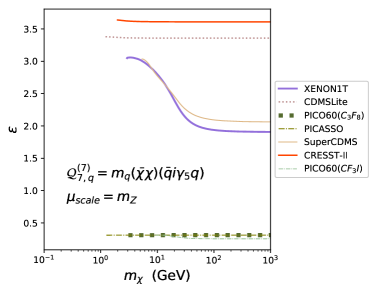
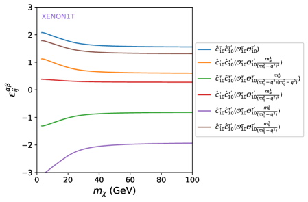
Figure 10: Parameter $\epsilon$ defined in Eq. (23) as a function of the WIMP mass $m_{\chi}$ for model ${\cal Q}^{(7)}_{7,q}$. (left) Parameter $\epsilon$ as a function of the WIMP mass $m_{\chi}$ for all the experiments and energy bins considered in Section 3. (right) Contributions $\epsilon_{ij}^{\alpha\beta}$ (each arising from one of the terms listed in Table 2) for the specific example of the XENON1T experiment.

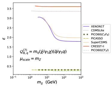
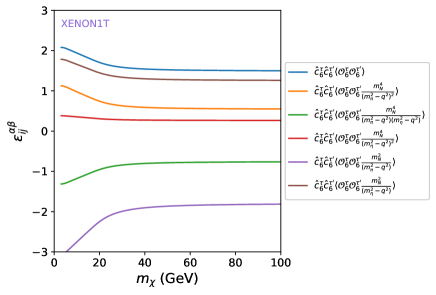
Figure 11: The same as in Fig. 10 for model ${\cal Q}^{(7)}_{8,q}$.

To discuss whether it is correct to assume dominance of one effective operator $F_{i}^{\alpha}(q^{2}){\cal O}_{i}$ at a time we introduce the parameters:

$$\epsilon_{ij}^{\alpha\beta}=\frac{\sum_{\tau\tau^{\prime}}\hat{c}_{i,\alpha}^{\tau}\hat{c}_{j,\beta}^{\tau^{\prime}}\langle{\cal O}_{i}{\cal O}_{j}F_{i}^{\alpha}(q^{2})F_{j}^{\beta}(q^{2})\rangle_{\tau\tau^{\prime}}}{\sum_{\tau\tau^{\prime}}\sum_{lm}\sum_{\rho\sigma}\hat{c}_{l,\rho}^{\tau}\hat{c}_{m,\sigma}^{\tau^{\prime}}\langle{\cal O}_{l}{\cal O}_{m}F_{l}^{\rho}(q^{2})F_{m}^{\sigma}(q^{2})\rangle_{\tau\tau^{\prime}}},\,\,\,\,\epsilon\equiv\max_{i,j,\alpha,\beta}(|\epsilon_{ij}^{\alpha\beta}|).$$ (23)

By numerical inspection we find that, with the exception of the operators ${\cal Q}^{(7)}_{7,q}$ and ${\cal Q}^{(7)}_{8,q}$, the $\epsilon$ parameter in all the energy bins of all the experiments included in our analysis never exceeds 1.7. Actually, we have checked that such extreme value (indicating destructive interference) corresponds to the highest energy bins of DAMA0 where the rate is exponentially suppressed by the velocity distribution and irrelevant for the constraint. In all other cases $\epsilon\mathrel{\mathop{\kern 0.0pt\hbox to0.0pt{\raise 0.86108pt\hbox{$<$}\hss}}\lower 3.87495pt\hbox{\kern-1.90002pt$\sim$}}$1.3. As a consequence, assuming dominance of one of the combinations $F_{i}^{\alpha}(q^{2}){\cal O}_{i}$ in the calculation of the expected rate in the determination of the exclusion plot implies an inaccuracy within $\pm\simeq$ 40-50 % for $\epsilon>1$ and a factor of 2 for $\epsilon<1$, but in most cases much smaller.

In Figs. 10 and 11 we plot $\epsilon$ as a function of the WIMP mass $m_{\chi}$ for the two operators ${\cal Q}^{(7)}_{7,q}$ and ${\cal Q}^{(7)}_{8,q}$. In particular, while the dominant contribution for ${\cal Q}^{(7)}_{3}$ and ${\cal Q}^{(7)}_{4}$ corresponds to the constant term in Eq.(11), as shown in Figs. 10 and 11 the situation is different for ${\cal Q}^{(7)}_{7}$ and ${\cal Q}^{(7)}_{8}$, where each of the terms ${\cal O}_{n}$,${\cal O}_{n}\frac{m_{N}^{2}}{m_{\pi}^{2}-q^{2}}$,${\cal O}_{n}\frac{m_{N}^{2}}{m_{\eta}^{2}-q^{2}}$ (with $n$=10,6) is of the same size with large cancellations among them (as indicated by $\epsilon\gg$ 1 values in the left–hand plot). This is confirmed by the right–hand plot of each of the two figures, where we show explicitly the $\epsilon_{ij}^{\alpha\beta}$ contributions for the specific example of the XENON1T experiment. Indeed for the interaction terms ${\cal Q}^{(7)}_{7}$ and ${\cal Q}^{(7)}_{8}$ such effect is natural since in this particular case the momentum–independent term ${\cal O}_{n}$ is next-to-leading order in chiral counting [49] compared to the terms ${\cal O}_{n}\frac{m_{N}^{2}}{m_{\pi}^{2}-q^{2}}$ and ${\cal O}_{n}\frac{m_{N}^{2}}{m_{\eta}^{2}-q^{2}}$.

Indeed, our conclusions on the $\epsilon$ parameter are not unexpected, since the scaling of the rate for different NR operators is very different, and depends also on experimental inputs, so barring accidental cancellations or clear–cut situations, like the one of axial operators ${\cal Q}^{(7)}_{7,q}$ and ${\cal Q}^{(7)}_{8,q}$, dominance of one NR operator appears natural. The numerical tests in this Section confirm this. In A we introduce

RDD_constraints }, a simple code that exploits this feature to
calculate approximate bounds on the couplings $\C^{(d)}_{a,q}$ and
$\C^{(d)}_{b}$. In particular, while the results of
Section~\ref{sec:analysis} have been obtained by assuming a single
coupling $\C_{a,q}^{(d)}$ common to all quarks, using
{\verb 

RDD_constraints such constraints can be generalized to a generic dependence of such couplings on the flavor $q$.

5 Conclusions

Assuming for WIMPs a Maxwellian velocity distribution in the Galaxy we have explored in a systematic way the relative sensitivity of an extensive set of existing DM direct detection experiments to each of the operators ${\cal Q}^{(d)}_{a,q}$, ${\cal Q}^{(d)}_{b}$ listed in Eqs. (3–5) up to dimension 7 describing dark matter effective interactions with quarks and gluons. In particular we have focused on a systematic approach, including an extensive set of experiments and large number of couplings, both exceeding for completeness similar analyses in the literature. For all the operators we have fixed the corresponding dimensional coupling ${\cal C}^{(d)}_{a,q}$ at the scale $\mu_{scale}$=$m_{Z}$ and used the code DirectDM [48] to perform the running from $m_{Z}$ to the nucleon scale and the hadronization to single-nucleon (N=p,n) currents, including QCD effects and pion poles that arise in the nonperturbative matching of the effective field theory to the low–energy Galilean–invariant nonrelativistic effective theory describing DM–nucleon interactions. For operators ${\cal Q}^{(6)}_{3,q}$ and ${\cal Q}^{(6)}_{4,q}$ we have also used the runDM code [69] to discuss the mixing effect among the vector and axial–vector currents induced by the running of the couplings above the EW scale, when the DM vector–axial coupling is assumed to be the same to all quarks.

We find that operators ${\cal Q}^{(5)}_{1,q}$, ${\cal Q}^{(5)}_{2,q}$, ${\cal Q}^{(6)}_{1,q}$, ${\cal Q}^{(6)}_{2,q}$, ${\cal Q}^{(7)}_{1}$, ${\cal Q}^{(7)}_{2}$, ${\cal Q}^{(7)}_{5,q}$, ${\cal Q}^{(7)}_{6,q}$ and ${\cal Q}^{(7)}_{10,q}$ take contributions which correspond to a Spin Independent scaling of the cross section (possibly combined with explicit dependence from the exchanged momentum $q^{2}$ and from the WIMP incoming speed) leading to an exclusion plot driven by DarkSide–50 at low WIMP mass and XENON1T at larger $m_{\chi}$. On the other hand for models ${\cal Q}^{(6)}_{3,q}$, ${\cal Q}^{(6)}_{4,q}$, ${\cal Q}^{(7)}_{3}$, ${\cal Q}^{(7)}_{4}$, ${\cal Q}^{(7)}_{7,q}$, ${\cal Q}^{(7)}_{8,q}$, and ${\cal Q}^{(7)}_{9,q}$ the cross section scaling law is of the Spin–Dependent type, leading to an exclusion plot driven by PICASSO and PICO60 (and, sometimes, by CDMSLite) at low WIMP mass, and by XENON1T at larger WIMP masses.

We also find that for models ${\cal Q}^{(7)}_{2}$, ${\cal Q}^{(7)}_{3}$, ${\cal Q}^{(7)}_{4}$, ${\cal Q}^{(7)}_{6}$, ${\cal Q}^{(7)}_{7}$, ${\cal Q}^{(7)}_{8}$ and ${\cal Q}^{(7)}_{9}$ the present experimental sensitivity of direct detection experiments appears not to be able to put bounds consistent to the validity of the EFT, although only matching the EFT with the full theory would allow to draw robust conclusions.

The matching between the relativistic effective theory to the NR one implies a redundancy of the parameters ${\cal C}^{(d)}_{a,q}$, implying that in many cases the DD constraints, that only depend on the ratio $c_{i}^{n}/c_{i}^{p}$ between the WIMP–neutron and the WIMP–proton couplings, can only be discussed for specific benchmarks. In particular in our exclusion plots we have assumed a flavor–independent coupling, ${\cal C}^{(d)}_{a,q}$=${\cal C}^{(d)}_{a}$. However, we have shown how, once the WIMP mass $m_{\chi}$ and the $c_{i}^{n}/c_{i}^{p}$ ratio are fixed, for all the ${\cal Q}^{(d)}_{a,q}$ models with the exception of ${\cal Q}^{(7)}_{7,q}$ and ${\cal Q}^{(7)}_{8,q}$ the expected rate is naturally driven by a dominant contribution from one of the NR operators ${\cal O}_{i}$ (possibly modified by a momentum–dependent Wilson coefficient, ${\cal O}_{i}\rightarrow{\cal O}_{i}F_{i}^{\alpha}(q^{2})$) without large cancellations. This implies that the bounds directly obtained within the context of the NR theory by assuming dominance of one of the $F_{i}^{\alpha}(q^{2}){O}_{i}$ can be used as discussed in Ref. [40] to obtain approximate constraints valid for any choice of the ${\cal Q}^{(d)}_{a,q}$ parameters, with an inaccuracy within a factor of two, but usually smaller. To perform such task in A we provide a simple interpolating interface in Python. On the other hand, in the case of ${\cal Q}^{(7)}_{7,q}$ and ${\cal Q}^{(7)}_{8,q}$ the terms with a momentum–independent coefficient ${\cal O}_{10}$ and ${\cal O}_{6}$ are next-to-leading order compared to the terms $F_{i}(q^{2}){\cal O}_{10}$ and $F_{i}(q^{2}){\cal O}_{6}$ which depend on the pion and eta propagators $F_{i}(q^{2})=1/(m_{\pi}^{2}-q^{2})$, $1/(m_{\eta}^{2}-q^{2})$, so that they cannot be assumed to dominate. Indeed, in this case all the terms $F_{n}(q^{2}){\cal O}_{n}$ are naturally of the same order with large cancellations among them.

Appendix A The program

The

RDD_constraints } code provides a simple interpolating
function written in Python that for a given generalized 

R diagonal term $(F_{i}^{\alpha})^{2}{\cal O}_{i}{\cal O}_{i}$ among those listed in Table 2 (with the exception of those proportional to a meson pole) calculates the most constraining limit among the experiments analyzed in [40] on the effective cross section:

$$\sigma^{\cal N}_{i,\alpha}=\max(\sigma^{p}_{i,\alpha},\sigma^{n}_{i,\alpha}),$$ (24)

(for $F_{i}^{\alpha}$=1,$(q^{2})^{-1}$) with:

$$\sigma^{p,n}_{i,\alpha}=(\hat{c}_{i,\alpha}^{p,n})^{2}\frac{\mu_{\chi{\cal N}}^{2}}{\pi},$$ (25)

as a function of the WIMP mass $m_{\chi}$ and of the ratio $r_{i}=\hat{c}_{i,\alpha}^{n}/\hat{c}_{i,\alpha}^{p}$. The $\hat{c}_{i,\alpha}^{p,n}$ coefficients are defined in Eq. (21). The code requires the

ciPy }
package and contains only four files, the code
{\verb NRDD_constraints.py }, two data files {\verb NRDD_data1.npy } and
{\verb NRDD_data2.npy }, and a driver template {\verb NRDD_constraints-example.py }.
The module can be downloaded from
\begin{center}
% \url{https://DD_NR_constraints.github.io}
{\verb https://github.com/NRDD-constraints/NRDD }
\end{center} or cloned by
\begin{Verbatim}[frame=single,xleftmargin=1cm,xrightmargin=1cm,commandchars=\\\{\}]
  git clone https://github.com/NRDD-constraints/NRDD
\end{Verbatim}
% and must be copied in the working directory.
By typing:
\begin{Verbatim}[frame=single,xleftmargin=1cm,xrightmargin=1cm,commandchars=\\\{\}]
  import NRDD_constraints as NR
\end{Verbatim}
\noindent two functions are defined. The function {\verb sigma_nucleon_bound(inter,mchi,r) }
returns the upper bound $(\sigma^{\cal  N}_{i,\alpha})_{lim}$ on the effective cross section of
Eq.(\ref{eq:conventional_sigma_nucleon}) in cm$^2$ as a function of
the WIMP mass {\verb mchi } and of the ratio {\verb r }=$r$ in the
ranges $0.1 \mbox{ GeV}<m_{\chi}<1000$ GeV, $-10^4 <r<10^4$.
The {\verb inter }
parameter is a string that selects the interaction term and
can be chosen in the list provided by the second function
{\verb print_interactions() }:
%   [’O12_O12’, ’O6_O6_qm4’, ’O14_O14’, ’O7_O7’, ’O4_O4’,\\
%     ’O13_O13’, ’O5_O5’, ’O8_O8’, ’O11_O11’, ’O9_O9’, \\
%     ’O3_O3’, ’O5_O5_qm4’, ’O10_O10’, ’O11_O11_qm4’, \\
%      ’O6_O6’, ’O1_O1’, ’O15_O15’]
\begin{Verbatim}[frame=single,xleftmargin=1cm,xrightmargin=1cm,commandchars=\\\{\}]
  NR.print_interactions()\\
  [’O1_O1’,’O3_O3’, ’O4_O4’, ’O5_O5’, ’O6_O6’,\\
   ’O7_O7’, ’O8_O8’, ’O9_O9’, ’O10_O10’, ’O11_O11’,\\
   ’O12_O12’, ’O13_O13’, ’O14_O14’, ’O15_O15’\\
   ’O5_O5_qm4’, ’O6_O6_qm4’, ’O11_O11_qm4’]
\end{Verbatim}
\noindent The list above includes all the $\op_i\op_i F_i^2(q^2)$
terms in Table~\ref{table:interferences} with the exception of those
depending on pion and eta poles which, as explained in

ection 4, are either subdominant in the case of models ${\cal Q}^{(7)}_{3}$ and ${\cal Q}^{(7)}_{4}$, or, in the case of ${\cal Q}^{(7)}_{7}$ and ${\cal Q}^{(7)}_{8}$, imply absence of a dominant term altogether (see Figs. 10 and 11) so that the procedure described in this Section leads to an inaccurate estimation of the constraints. This can be seen explicitly in Fig. 8, where the red–dashed curve approximates poorly the bound obtained with a full calculation. The upper bound returned by igma_nucleon_bound(inter,mchi,r) } correponds to the results of  [40] with the exception of the interaction terms with momentum dependence in the Wilson coefficient, that have been added to include the long–range interactions of Eq.(3).

The driver

RDD_constraints-example.py } calculates the
exclusion plot on the reference cross section:
\begin{equation}
\sigma^{rel}_{ref}=\C^2 \frac{\mu_{\chi{\cal 

^2π,

assuming for the interaction between the DM particle $\chi$ and the nucleon $\Psi_{N}$ the relativistic effective Lagrangian:

$${\cal L}={\cal C}\bar{\chi}\gamma^{\mu}\chi\Psi_{N}\gamma_{\mu}\gamma_{5}\Psi_{N}\rightarrow{\cal C}\sum_{N=p,n}\left(c^{N}_{7}{\cal O}_{7}^{N}+c^{N}_{9}{\cal O}_{9}^{N}\right),$$ (26)

with $c^{p}_{7}$=-2, $c^{p}_{9}$=$2m_{N}/m_{\chi}$ and $r_{i}$=$c^{n}_{i}/c^{p}_{i}$. Assuming dominance of one operator ${\cal O}_{i}$ at a time the driver implements a function oeff(inter,mhi,r) that calculates the largest Wilson coefficient between proton and neutron in absolute value $max(|c_{i}^{p}(m_{\chi},r)|,|c_{i}^{n}(m_{\chi},r)|)$ and plots the bound $(\sigma^{rel}_{ref})_{lim}$ on $\sigma^{rel}_{ref}$ as [40]:

$$(\sigma^{rel}_{ref})_{lim}=\min_{i=7,9}\left(\frac{(\sigma^{\cal N}_{i})_{lim}(m_{\chi},r_{i})}{max(c_{i}^{p}(m_{\chi},r_{i})^{2},c_{i}^{n}(m_{\chi},r_{i})^{2})}\right),$$ (27)

for the specific choice $r_{7}$=$r_{9}$=1. In particular, for a given value of the WIMP mass

chi }:
\begin{Verbati

[frame=single,xleftmargin=1cm,xrightmargin=1cm,commandchars=
{}] sigma_lim_rel_min=large_number
for inter in [’O7_O7’,’O9_O9’]:
c=coeff(inter,mchi,r)
sigma_lim_nucleon_NR=NR.sigma_nucleon_bound(inter,mchi,r)
sigma_lim_rel=sigma_lim_nucleon_NR/c**2
sigma_lim_rel_min=min(sigma_lim_rel_min,sigma_lim_rel)

Such limit is also converted into an upper bound $(\tilde{\Lambda})_{lim}$ in GeV on $\tilde{\Lambda}$ using:

$$(\tilde{\Lambda})_{lim}=\left(\frac{\mu_{\chi{\cal N}}(\hbar c)}{\sqrt{(\sigma^{rel}_{ref})_{lim}\pi}}\right)^{\frac{1}{d-4}},$$ (28)

with $\hbar c$=1.97$\times 10^{-14}$ cm GeV and $d$=6 the dimension of the considered operator. An analogous procedure allows to obtain the red–dashed curve in Figs. 1–3 and Figs. 5–9 that reproduce accurately most of the results of Section 3.

References

- [1]
- [2] P. A. R. Ade, et al., Planck 2013 results. XVI. Cosmological parameters, Astron. Astrophys. 571 (2014) A16. arXiv:1303.5076, doi:10.1051/0004-6361/201321591.
- [3] R. Bernabei, et al., Searching for WIMPs by the annual modulation signature, Phys. Lett. B424 (1998) 195–201. doi:10.1016/S0370-2693(98)00172-5.
- [4] R. Bernabei, et al., First results from DAMA/LIBRA and the combined results with DAMA/NaI, Eur. Phys. J. C56 (2008) 333–355. arXiv:0804.2741, doi:10.1140/epjc/s10052-008-0662-y.
- [5] R. Bernabei, et al., New results from DAMA/LIBRA, Eur. Phys. J. C67 (2010) 39–49. arXiv:1002.1028, doi:10.1140/epjc/s10052-010-1303-9.
- [6] R. Bernabei, et al., First Model Independent Results from DAMA/LIBRA–Phase2, Universe 4 (11) (2018) 116, [At. Energ.19,307(2018)]. arXiv:1805.10486, doi:10.3390/universe4110116,10.15407/jnpae2018.04.307.
- [7] E. Aprile, et al., Dark Matter Search Results from a One Ton-Year Exposure of XENON1T, Phys. Rev. Lett. 121 (11) (2018) 111302. arXiv:1805.12562, doi:10.1103/PhysRevLett.121.111302.
- [8] X. Cui, et al., Dark Matter Results From 54-Ton-Day Exposure of PandaX-II Experiment, Phys. Rev. Lett. 119 (18) (2017) 181302. arXiv:1708.06917, doi:10.1103/PhysRevLett.119.181302.
- [9] H. S. Lee, et al., Search for Low-Mass Dark Matter with CsI(Tl) Crystal Detectors, Phys. Rev. D90 (5) (2014) 052006. arXiv:1404.3443, doi:10.1103/PhysRevD.90.052006.
- [10] R. Agnese, et al., Low-mass dark matter search with CDMSlite, Phys. Rev. D97 (2) (2018) 022002. arXiv:1707.01632, doi:10.1103/PhysRevD.97.022002.
- [11] R. Agnese, et al., Results from the Super Cryogenic Dark Matter Search Experiment at Soudan, Phys. Rev. Lett. 120 (6) (2018) 061802. arXiv:1708.08869, doi:10.1103/PhysRevLett.120.061802.
- [12] E. Behnke, et al., First Dark Matter Search Results from a 4-kg CF3I Bubble Chamber Operated in a Deep Underground Site, Phys. Rev. D86 (5) (2012) 052001, [Erratum: Phys. Rev.D90,no.7,079902(2014)]. arXiv:1204.3094, doi:10.1103/PhysRevD.86.052001,10.1103/PhysRevD.90.079902.
- [13] E. Behnke, et al., Final Results of the PICASSO Dark Matter Search Experiment, Astropart. Phys. 90 (2017) 85–92. arXiv:1611.01499, doi:10.1016/j.astropartphys.2017.02.005.
- [14] C. Amole, et al., Dark Matter Search Results from the PICO-60 CF3I Bubble Chamber, Submitted to: Phys. Rev. DarXiv:1510.07754.
- [15] C. Amole, et al., Dark Matter Search Results from the Complete Exposure of the PICO-60 C3F8 Bubble ChamberarXiv:1902.04031.
- [16] G. Angloher, et al., Results on light dark matter particles with a low-threshold CRESST-II detector, Eur. Phys. J. C76 (1) (2016) 25. arXiv:1509.01515, doi:10.1140/epjc/s10052-016-3877-3.
- [17] L. T. Yang, et al., Limits on light WIMPs with a 1 kg-scale germanium detector at 160 eVee physics threshold at the China Jinping Underground Laboratory, Chin. Phys. C42 (2) (2018) 023002. arXiv:1710.06650, doi:10.1088/1674-1137/42/2/023002.
- [18] A. Aguilar-Arevalo, et al., Search for low-mass WIMPs in a 0.6 kg day exposure of the DAMIC experiment at SNOLAB, Phys. Rev. D94 (8) (2016) 082006. arXiv:1607.07410, doi:10.1103/PhysRevD.94.082006.
- [19] P. Agnes, et al., Low-mass Dark Matter Search with the DarkSide-50 ExperimentarXiv:1802.06994.
- [20] G. Arcadi, M. Dutra, P. Ghosh, M. Lindner, Y. Mambrini, M. Pierre, S. Profumo, F. S. Queiroz, The waning of the WIMP? A review of models, searches, and constraints, Eur. Phys. J. C78 (3) (2018) 203. arXiv:1703.07364, doi:10.1140/epjc/s10052-018-5662-y.
- [21] C. Kelso, C. Savage, M. Valluri, K. Freese, G. S. Stinson, J. Bailin, The impact of baryons on the direct detection of dark matter, JCAP 1608 (2016) 071. arXiv:1601.04725, doi:10.1088/1475-7516/2016/08/071.
- [22] A. M. Green, Astrophysical uncertainties on direct detection experiments, Mod. Phys. Lett. A27 (2012) 1230004. arXiv:1112.0524, doi:10.1142/S0217732312300042.
- [23] A. L. Fitzpatrick, W. Haxton, E. Katz, N. Lubbers, Y. Xu, The Effective Field Theory of Dark Matter Direct Detection, JCAP 1302 (2013) 004. arXiv:1203.3542, doi:10.1088/1475-7516/2013/02/004.
- [24] N. Anand, A. L. Fitzpatrick, W. C. Haxton, Weakly interacting massive particle-nucleus elastic scattering response, Phys. Rev. C89 (6) (2014) 065501. arXiv:1308.6288, doi:10.1103/PhysRevC.89.065501.
- [25] S. Chang, A. Pierce, N. Weiner, Momentum Dependent Dark Matter Scattering, JCAP 1001 (2010) 006. arXiv:0908.3192, doi:10.1088/1475-7516/2010/01/006.
- [26] B. A. Dobrescu, I. Mocioiu, Spin-dependent macroscopic forces from new particle exchange, JHEP 11 (2006) 005. arXiv:hep-ph/0605342, doi:10.1088/1126-6708/2006/11/005.
- [27] J. Fan, M. Reece, L.-T. Wang, Non-relativistic effective theory of dark matter direct detection, JCAP 1011 (2010) 042. arXiv:1008.1591, doi:10.1088/1475-7516/2010/11/042.
- [28] R. J. Hill, M. P. Solon, WIMP-nucleon scattering with heavy WIMP effective theory, Phys. Rev. Lett. 112 (2014) 211602. arXiv:1309.4092, doi:10.1103/PhysRevLett.112.211602.
- [29] V. Gluscevic, A. H. G. Peter, Understanding WIMP-baryon interactions with direct detection: A Roadmap, JCAP 1409 (09) (2014) 040. arXiv:1406.7008, doi:10.1088/1475-7516/2014/09/040.
- [30] M. Cirelli, E. Del Nobile, P. Panci, Tools for model-independent bounds in direct dark matter searches, JCAP 1310 (2013) 019. arXiv:1307.5955, doi:10.1088/1475-7516/2013/10/019.
- [31] S. Chang, R. Edezhath, J. Hutchinson, M. Luty, Effective WIMPs, Phys. Rev. D89 (1) (2014) 015011. arXiv:1307.8120, doi:10.1103/PhysRevD.89.015011.
- [32] R. Catena, Prospects for direct detection of dark matter in an effective theory approach, JCAP 1407 (2014) 055. arXiv:1406.0524, doi:10.1088/1475-7516/2014/07/055.
- [33] R. Catena, Dark matter directional detection in non-relativistic effective theories, JCAP 1507 (07) (2015) 026. arXiv:1505.06441, doi:10.1088/1475-7516/2015/07/026.
- [34] R. Catena, P. Gondolo, Global fits of the dark matter-nucleon effective interactions, JCAP 1409 (09) (2014) 045. arXiv:1405.2637, doi:10.1088/1475-7516/2014/09/045.
- [35] K. Schneck, et al., Dark matter effective field theory scattering in direct detection experiments, Phys. Rev. D91 (9) (2015) 092004. arXiv:1503.03379, doi:10.1103/PhysRevD.91.092004.
- [36] R. Catena, P. Gondolo, Global limits and interference patterns in dark matter direct detection, JCAP 1508 (08) (2015) 022. arXiv:1504.06554, doi:10.1088/1475-7516/2015/08/022.
- [37] H. Rogers, D. G. Cerdeno, P. Cushman, F. Livet, V. Mandic, Multidimensional effective field theory analysis for direct detection of dark matter, Phys. Rev. D95 (8) (2017) 082003. arXiv:1612.09038, doi:10.1103/PhysRevD.95.082003.
- [38] E. Aprile, et al., Effective field theory search for high-energy nuclear recoils using the XENON100 dark matter detector, Phys. Rev. D96 (4) (2017) 042004. arXiv:1705.02614, doi:10.1103/PhysRevD.96.042004.
- [39] G. Angloher, et al., Limits on Dark Matter Effective Field Theory Parameters with CRESST-II, Eur. Phys. J. C79 (1) (2019) 43. arXiv:1809.03753, doi:10.1140/epjc/s10052-018-6523-4.
- [40] S. Kang, S. Scopel, G. Tomar, J.-H. Yoon, Present and projected sensitivities of Dark Matter direct detection experiments to effective WIMP-nucleus couplings, Astropart. Phys. 109 (2019) 50–68. arXiv:1805.06113, doi:10.1016/j.astropartphys.2019.02.006.
-
[41]
S. Yellin, Finding
an upper limit in the presence of an unknown background, Phys. Rev. D 66
(2002) 032005.
doi:10.1103/PhysRevD.66.032005.
URL https://link.aps.org/doi/10.1103/PhysRevD.66.032005 - [42] F. D’Eramo, M. Procura, Connecting Dark Matter UV Complete Models to Direct Detection Rates via Effective Field Theory, JHEP 04 (2015) 054. arXiv:1411.3342, doi:10.1007/JHEP04(2015)054.
- [43] F. D’Eramo, B. J. Kavanagh, P. Panci, You can hide but you have to run: direct detection with vector mediators, JHEP 08 (2016) 111. arXiv:1605.04917, doi:10.1007/JHEP08(2016)111.
- [44] A. Belyaev, E. Bertuzzo, C. Caniu Barros, O. Eboli, G. Grilli Di Cortona, F. Iocco, A. Pukhov, Interplay of the LHC and non-LHC Dark Matter searches in the Effective Field Theory approach, Phys. Rev. D99 (1) (2019) 015006. arXiv:1807.03817, doi:10.1103/PhysRevD.99.015006.
- [45] E. Masso, S. Mohanty, S. Rao, Dipolar Dark Matter, Phys. Rev. D80 (2009) 036009. arXiv:0906.1979, doi:10.1103/PhysRevD.80.036009.
- [46] E. Del Nobile, G. B. Gelmini, P. Gondolo, J.-H. Huh, Direct detection of Light Anapole and Magnetic Dipole DM, JCAP 1406 (2014) 002. arXiv:1401.4508, doi:10.1088/1475-7516/2014/06/002.
- [47] J. Engel, S. Pittel, P. Vogel, Nuclear physics of dark matter detection, Int. J. Mod. Phys. E1 (1992) 1–37. doi:10.1142/S0218301392000023.
- [48] F. Bishara, J. Brod, B. Grinstein, J. Zupan, DirectDM: a tool for dark matter direct detectionarXiv:1708.02678.
- [49] F. Bishara, J. Brod, B. Grinstein, J. Zupan, From quarks to nucleons in dark matter direct detection, JHEP 11 (2017) 059. arXiv:1707.06998, doi:10.1007/JHEP11(2017)059.
- [50] J. Goodman, M. Ibe, A. Rajaraman, W. Shepherd, T. M. P. Tait, H.-B. Yu, Constraints on Dark Matter from Colliders, Phys. Rev. D82 (2010) 116010. arXiv:1008.1783, doi:10.1103/PhysRevD.82.116010.
- [51] M. R. Buckley, Using Effective Operators to Understand CoGeNT and CDMS-Si Signals, Phys. Rev. D88 (5) (2013) 055028. arXiv:1308.4146, doi:10.1103/PhysRevD.88.055028.
- [52] A. De Simone, T. Jacques, Simplified models vs. effective field theory approaches in dark matter searches, Eur. Phys. J. C76 (7) (2016) 367. arXiv:1603.08002, doi:10.1140/epjc/s10052-016-4208-4.
- [53] M. I. Gresham, K. M. Zurek, Effect of nuclear response functions in dark matter direct detection, Phys. Rev. D89 (12) (2014) 123521. arXiv:1401.3739, doi:10.1103/PhysRevD.89.123521.
- [54] V. Gluscevic, M. I. Gresham, S. D. McDermott, A. H. G. Peter, K. M. Zurek, Identifying the Theory of Dark Matter with Direct Detection, JCAP 1512 (12) (2015) 057. arXiv:1506.04454, doi:10.1088/1475-7516/2015/12/057.
- [55] G. Angloher, et al., Description of CRESST-II dataarXiv:1701.08157.
- [56] R. Bernabei, et al., The DAMA/LIBRA apparatus, Nucl. Instrum. Meth. A592 (2008) 297–315. arXiv:0804.2738, doi:10.1016/j.nima.2008.04.082.
- [57] C. Amole, et al., Dark Matter Search Results from the PICO-60 C3F8 Bubble Chamber, Phys. Rev. Lett. 118 (25) (2017) 251301. arXiv:1702.07666, doi:10.1103/PhysRevLett.118.251301.
- [58] A. Belyaev, E. Bertuzzo, C. Caniu Barros, O. Eboli, G. Grilli Di Cortona, F. Iocco, A. Pukhov, Interplay of the LHC and non-LHC Dark Matter searches in the Effective Field Theory approach, Phys. Rev. D99 (1) (2019) 015006. arXiv:1807.03817, doi:10.1103/PhysRevD.99.015006.
- [59] K. Schneck, et al., Dark matter effective field theory scattering in direct detection experiments, Phys. Rev. D91 (9) (2015) 092004. arXiv:1503.03379, doi:10.1103/PhysRevD.91.092004.
- [60] C. Arina, E. Del Nobile, P. Panci, Dark Matter with Pseudoscalar-Mediated Interactions Explains the DAMA Signal and the Galactic Center Excess, Phys. Rev. Lett. 114 (2015) 011301. arXiv:1406.5542, doi:10.1103/PhysRevLett.114.011301.
- [61] A. Belyaev, E. Bertuzzo, C. Caniu Barros, O. Eboli, G. Grilli Di Cortona, F. Iocco, A. Pukhov, Interplay of the LHC and non-LHC Dark Matter searches in the Effective Field Theory approacharXiv:1807.03817.
- [62] R. J. Hill, M. P. Solon, Universal behavior in the scattering of heavy, weakly interacting dark matter on nuclear targets, Phys. Lett. B707 (2012) 539–545. arXiv:1111.0016, doi:10.1016/j.physletb.2012.01.013.
- [63] R. J. Hill, M. P. Solon, WIMP-nucleon scattering with heavy WIMP effective theory, Phys. Rev. Lett. 112 (2014) 211602. arXiv:1309.4092, doi:10.1103/PhysRevLett.112.211602.
- [64] M. Hoferichter, P. Klos, A. Schwenk, Chiral power counting of one- and two-body currents in direct detection of dark matter, Phys. Lett. B746 (2015) 410–416. arXiv:1503.04811, doi:10.1016/j.physletb.2015.05.041.
- [65] M. Hoferichter, P. Klos, J. Menéndez, A. Schwenk, Analysis strategies for general spin-independent WIMP-nucleus scattering, Phys. Rev. D94 (6) (2016) 063505. arXiv:1605.08043, doi:10.1103/PhysRevD.94.063505.
- [66] J. Brod, A. Gootjes-Dreesbach, M. Tammaro, J. Zupan, Effective Field Theory for Dark Matter Direct Detection up to Dimension Seven, JHEP 10 (2018) 065. arXiv:1710.10218, doi:10.1007/JHEP10(2018)065.
- [67] E. Del Nobile, A complete Lorentz-to-Galileo dictionary for direct Dark Matter detectionarXiv:1806.01291.
- [68] S. Kang, S. Scopel, G. Tomar, J.-H. Yoon, P. Gondolo, Anapole Dark Matter after DAMA/LIBRA-phase2, JCAP 1811 (11) (2018) 040. arXiv:1808.04112, doi:10.1088/1475-7516/2018/11/040.
-
[69]
F. D’Eramo, B. J. Kavanagh, P. Panci, runDM (Version 1.1) [Computer
software],
https://github.com/bradkav/runDM/ - [70] R. Catena, B. Schwabe, Form factors for dark matter capture by the Sun in effective theories, JCAP 1504 (04) (2015) 042. arXiv:1501.03729, doi:10.1088/1475-7516/2015/04/042.
- [71] Z. Ahmed, et al., Analysis of the low-energy electron-recoil spectrum of the CDMS experiment, Phys. Rev. D81 (2010) 042002. arXiv:0907.1438, doi:10.1103/PhysRevD.81.042002.
- [72] G. Angloher, et al., Description of CRESST-II dataarXiv:1701.08157.