K3 surfaces from configurations of six lines in $\mathbb{P}^{2}$ and mirror symmetry I

Abstract.

From the viewpoint of mirror symmetry, we revisit the hypergeometric system $E(3,6)$ for a family of K3 surfaces. We construct a good resolution of the Baily-Borel-Satake compactification of its parameter space, which admits special boundary points (LCSLs) given by normal crossing divisors. We find local isomorphisms between the $E(3,6)$ systems and the associated GKZ systems defined locally on the parameter space and cover the entire parameter space. Parallel structures are conjectured in general for hypergeometric system $E(n,m)$ on Grassmannians. Local solutions and mirror symmetry will be described in a companion paper [18], where we introduce a K3 analogue of the elliptic lambda function in terms of genus two theta functions.

1. Introduction

Consider double covers of $\mathbb{P}^{1}$ branched along four points in general positions. They define a family of elliptic curves called the Legendre family over the moduli space of the configurations of four points on $\mathbb{P}^{1}$, which are naturally parametrized by the cross ratio of the four points. It is a classical fact that the elliptic lambda function is defined as a modular function that arises from the hypergeometric series representing period integrals for the Legendre family.

Higher dimensional analogues of the Legendre family have been studied in many context in the history of modular forms and analysis related to them. Among others, Matsumoto, Sasaki and Yoshida [22] have studied extensively in the 90’s the two dimensional generalization of the Legendre family, i.e., the double covers of the projective plane $\mathbb{P}^{2}$ branched along six lines in general positions. After making suitable resolutions, the double covers define a family of smooth K3 surfaces parametrized by the configurations of six lines. In [22], the authors studied in great details the period integrals of the family and determined the monodromy properties of the period integrals completely. They described the set of the differential equations satisfied by the period integrals in terms of the so-called Aomoto-Gel’fand system [1, 9, 8] on Grassmannians $G(3,6)$, and named them hypergeometric system $E(3,6)$.

Around the same time in the 90’s, period integrals for families of Calabi-Yau manifolds were studied intensively to verify several predictions from mirror symmetry of Calabi-Yau manifolds. For Calabi-Yau manifolds given as complete intersections in a toric variety, it is now known that the period integrals for such a family are solutions to a hypergeometric system called Gel’fand-Kapranov-Zelevinski (GKZ) system. In particular, it was shown in [17, 16] that for GKZ systems in this context there exist special boundary points called large complex structure limits (LCSLs), and mirror symmetry appears nicely in the form of generalized Frobenius method which provides a closed formula for period integrals and mirror map near these boundary points.

In this paper, we will revisit the hypergeometric system $E(3,6)$ from the viewpoint of mirror symmetry of K3 surfaces. Despite the fact that many analytic properties of $E(3,6)$ have been studied in details in the literature e.g. [22, 25], it was not clear how to construct the degeneration points (LCSLs) in the parameter space of $E(3,6)$. We will find that the $\mathcal{D}$-module associated to the hypergeometric system $E(3,6)$ over its parameter space is locally trivialized by the $\mathcal{D}$-module of the corresponding GKZ hypergeometric system (Theorem 7.1). Thanks to this general property, it turns out that the techniques developed in [17, 16] for GKZ systems can be applied to $E(3,6)$ (Theorem 7.2); this includes the existence of the degeneration points and the closed formula of the period integrals around them. To show our results, we first cover the parameter space of $E(3,6)$, which can be identified with the Baily-Borel-Satake compactification of the family of the K3 surfaces, by certain Zariski open subsets of toric varieties on which GKZ systems are defined. Using this covering property, we finally show that there are two nice algebraic resolutions of the Baily-Borel-Satake compactification (Theorem 6.12) which are related by a four dimensional flip.

Around the special degeneration points (LCSLs), following [17, 16], we can define the so-called mirror maps. In our case, these mirror maps can be regarded as two dimensional generalizations of the elliptic lambda function. We will call them $\lambda_{K3}$-functions. In a companion paper [18], we will describe the $\lambda_{K3}$-functions in terms of genus two theta functions. Moreover, we will find that, corresponding to the two different algebraic resolutions related by a flip, there exist two different definitions for the $\lambda_{K3}$-functions.

Here is the outline of this paper: In Section 2, after introducing our family of K3 surfaces and the hypergeometric system $E(3,6)$ satisfied by period integrals, we will introduce the configuration space of six ordered points as the parameter space of $E(3,6)$. We summarize known properties about the compactification of the parameter space of $E(3,6)$ and also introduce other closely related parameter spaces: the configuration space of 3 points and 3 lines in $\mathbb{P}^{2}$ and the parameter space of the GKZ system which trivializes the $E(3,6)$. In Section 3, we describe a toric compactification of the parameter space of this GKZ system, and construct the expected LCSLs after making a resolution. In Section 4, we observe that the configuration space of 3 points and 3 lines in $\mathbb{P}^{2}$ arises naturally from certain residue calculations of a period integral. We find that the toric compactification for the GKZ system gives a toric partial resolution of the GIT compactification of the configuration space of 3 points and 3 lines in $\mathbb{P}^{2}$. In Section 5 and 6, we reconstruct the partial resolution using classical projective geometry. Transforming this partial resolution (locally) by certain birational map to the Baily-Borel-Satake compactification, we construct the desired algebraic resolutions of the Baily-Borel-Satake compactification. In Section 7, we combine the results of the preceding sections and rephrase them in the language of $\mathcal{D}$-modules to state the main results of this paper. We also formulate conjectural generalizations of our results.

Acknowledgements: This project was initiated by a question by Naichung C. Leung about hypergeometric systems on Grassmannians to S.H. We are grateful to him for asking the question which actually has drawn our attention to the problems left unsolved in the 90’s. We are also grateful to Osamu Fujino for useful advice to the proof of Claim E.1. S.H. would like to thank for the warm hospitality at the CMSA at Harvard University where progress was made. This work is supported in part by Grant-in Aid Scientific Research (C 16K05105, S 17H06127, A 18H03668 S.H. and C 16K05090 H.T.). B.H.L and S.-T. Yau are supported by the Simons Collaboration Grant on Homological Mirror Symmetry and Applications 2015–2019.

2. The hypergeometric system $E(3,6)$

2.1. Double covering of $\mathbb{P}^{2}$ branched along six lines

Let us consider six lines $\ell_{i}(i=1,..,6)$ in $\mathbb{P}^{2}$ in general position. We denote them by $\left\{\ell_{i}({\tt x},{\tt y},{\tt z})=0\right\}\subset\mathbb{P}^{2}$ with the following linear forms:

$$\ell_{i}({\tt x},{\tt y},{\tt z}):=a_{0i}{\tt z}+a_{1i}{\tt x}+a_{2i}{\tt y}\;\;(i=1,...,6).$$

When the lines are in general position, the double cover branched along the six lines defines a singular K3 surface with $A_{1}$ singularity at each 15 intersection points $P_{ij}:=\ell_{i}\cap\ell_{j}$. Blowing-up the 15 $A_{1}$ singularities, we have a smooth K3 surface $X$ of Picard number 16 generated by the hyperplane class $H$ from $\mathbb{P}^{2}$ and the $-2$ curves of the exceptional divisors $E_{ij}$ from the blow-up. The configurations of six lines define a four dimensional family of K3 surfaces, which we will call double cover family of K3 surfaces for short in this paper. The period integrals of the family of holomorphic two forms and their monodromy properties were studied extensively in [22] by analyzing the hypergeometric system $E(3,6)$. We will revisit the system $E(3,6)$ from the viewpoint of mirror symmetry and provide a new perspective for mirror symmetry.

2.2. Period integrals of $X$

Recall that the Legendre family consists of elliptic curves given by double covers of $\mathbb{P}^{1}$ branched along four points in general position. The double cover family of K3 surfaces is a natural generalization of the Legendre family. Analogous to the period integrals of the Legendre family [29, Chap.IV,10] are the period integrals of a holomorphic two form:

(2.1) $$\bar{\omega}_{C}(a)=\int_{C}\frac{d\mu}{\sqrt{\prod_{i=1}^{6}\ell_{i}({\tt x},{\tt y},{\tt z})}},$$

where $d\mu={\tt x}d{\tt y}\wedge d{\tt z}-{\tt y}d{\tt x}\wedge d{\tt z}+{\tt z}d{\tt x}\wedge d{\tt y}$ and $C$ is an integral (transcendental) cycle in $H_{2}(X,\mathbb{Z}$). Explicit descriptions of the transcendental cycles can be found in [22]. Also the lattice of transcendental cycles is determined to be

$$T_{X}\simeq U(2)\oplus U(2)\oplus A_{1}\oplus A_{1},$$

where $U$(2) represents the hyperbolic lattice $U$ of rank 2 with the Gram matrix multiplied by 2, and $A_{1}=\langle-2\rangle$ is the root lattice of $sl(2,\mathbb{C})$. As obvious in the above definition, the period integrals $\bar{\omega}_{C}(a)$ determine (multi-valued) functions defined on the set of $3\times 6$ matrices $A$ representing (ordered) six lines in general positions. Explicitly, we describe the matrices $A$ by

(2.2) $$A=\left(\begin{matrix}a_{01}&a_{02}&a_{03}&a_{04}&a_{05}&a_{06}\\ a_{11}&a_{12}&a_{13}&a_{14}&a_{15}&a_{16}\\ a_{21}&a_{22}&a_{23}&a_{24}&a_{25}&a_{26}\end{matrix}\right).$$

Let $M_{3,6}$ be the affine space of all $3\times 6$ matrices, and set

$$M_{3,6}^{o}:=\left\{A\in M_{3,6}\mid D(i_{1},i_{2},i_{3})\not=0\,(1\leq i_{1}<i_{2}<i_{3}\leq 6)\right\}$$

with $D(i_{1},i_{2},i_{3})$ representing $3\times 3$ minors of $A$. Then, under the genericity assumption, the configurations of six lines are parametrized by

$$P(3,6):=GL(3,\mathbb{C})\diagdown M_{3,6}^{o}\diagup(\mathbb{C}^{*})^{6},$$

where $(\mathbb{C}^{*})^{6}$ represents the diagonal $\mathbb{C}^{*}$-actions. The differential operators which annihilate the period integrals define the hypergeometric system of type $E(3,6)$ [22, Sect.1.4], which is the Aomoto-Gel’fand system on Grassmannian $G(3,6)$ [1, 9, 8]. The following proposition is easy to derive.

Proposition 2.1.

The period integral $\bar{\omega}(a)$ satisfies the following set of differential equations:

(2.3) $$(\mathrm{i}) \;\;\sum_{i=0}^{2}a_{ij}\frac{\partial\;}{\partial a_{ij}}\bar{\omega}(a)=-\frac{1}{2}\bar{\omega}(a), 1\leq j\leq 6,$$

$$(\mathrm{ii}) \;\;\sum_{j=1}^{6}a_{ij}\frac{\partial\;}{\partial a_{kj}}\bar{\omega}(a)=-\delta_{ik}\bar{\omega}(a) 1\leq i\leq 3,$$

$$(\mathrm{iii}) \;\;\frac{\partial^{2}\;}{\partial a_{ij}\partial a_{kl}}\bar{\omega}(a)=\frac{\partial^{2}\;}{\partial a_{il}\partial a_{kj}}\bar{\omega}(a), \;\;\;1\leq i,k\leq 3,\;1\leq j,l\leq 6.$$

Proof.

The relations (i) and (iii) are rather easy to verify by differentiating (2.1) directly. To derive (ii), we note that $d\mu=i_{E}d{\tt x}\wedge d{\tt y}\wedge d{\tt z}$ holds with the Euler vector field $E={\tt x}\frac{\partial\;}{\partial{\tt x}}+{\tt y}\frac{\partial\;}{\partial{\tt y}}+{\tt z}\frac{\partial\;}{\partial{\tt z}}$. Since the Euler vector field is invariant under the linear coordinate transformation, it is easy to verify

$$\bar{\omega}(ga)=(\det g)^{-1}\bar{\omega}(a),$$

for the left $GL(3,\mathbb{C})$-action on $A=(a_{ij})\in M_{3,6}^{o}$. The relation follows from the infinitesimal form of this relation. ∎

In the paper [22], the hypergeometric functions representing the period integrals has been studied in details using the following affine coordinate system of the quotient $P(3,6)$:

$$\left(\begin{matrix}1&0&0&1&1&1\\ 0&1&0&1&x_{1}&x_{2}\\ 0&0&1&1&x_{3}&x_{4}\end{matrix}\right).$$

However, this affine coordinate turns out to be inadequate for studying mirror symmetry. In particular, in order to construct the special boundary points, called large complex structure limits (LCSLs), we need a suitable compactification.

2.3. Period domain and compactifications of the parameter space $P(3,6)$

Mirror symmetry for two or three dimensional Calabi-Yau hypersurfaces or complete intersections in toric Fano varieties was worked out in many examples in the 90’s by constructing families of Calabi-Yau manifolds and by studying period integrals associated to holomorphic $n$-forms for $n=2$ or $3$. It is now known that the geometry of mirror symmetry appears, in a certain simplified form [27], near the special boundary points which are given as normal crossing boundary divisors in suitable compactifications of the parameter spaces for the families of hypersurfaces [17]. The double cover family of K3 surfaces does not belong to these well-studied families of Calabi-Yau manifolds. However, its parameter space $P(3,6)$ admits many nice compactifications relevant to describe the boundary points. We summarize several compactifications and describe their relationships.

(2.3.a) Period domain ${\mathcal{D}}_{K3}=\Omega(U(2)^{\oplus 2}\oplus A_{1}^{\oplus 2})$. Since the generic member $X$ of the double cover family of K3 surfaces has the transcendental lattice $T_{X}\simeq U(2)^{\oplus 2}\oplus A_{1}^{\oplus 2},$ the period integral defines a map from $P(3,6)$ to the period domain

$$\mathcal{D}_{K3}:=\left\{[\omega]\in\mathbb{P}((U(2)^{\oplus 2}\oplus A_{1}^{\oplus 2})\otimes\mathbb{C})\mid\omega.\omega=0,\omega.\bar{\omega}>0\right\}^{+},$$

where ⁺ represents one of the connected components. Let us denote by $G$ the Gram matrix of the lattice $U(2)^{\oplus 2}\oplus A_{1}^{\oplus 2}$ given in the following block-diagonal from:

$$G=\left(\begin{matrix}0&2\\ 2&0\end{matrix}\right)\oplus\left(\begin{matrix}0&2\\ 2&0\end{matrix}\right)\oplus(-2)\oplus(-2).$$

Using this, we define

$$\mathcal{G}:=\left\{g\in PGL(6,\mathbb{Z})\mid\,^{t}gGg=G,H(g)>0\right\}$$

with $H(g)=(g_{11}+g_{12})(g_{33}+g_{34})-(g_{13}+g_{14})(g_{31}+g_{32})$, which is a discrete subgroup of $\mathrm{Aut}(\mathcal{D}_{K3}$) (see [21, Sect.1.4]). In [22, Prop.2.7.3], it is shown that the monodromy group of period integrals coincides with the congruence subgroup $\mathcal{G}(2)=\left\{g\in\mathcal{G}\mid g\equiv E_{6}\text{ mod }2\right\}$, hence $P(3,6)\simeq\mathcal{D}_{K3}/\mathcal{G}(2)$ holds and $\mathcal{D}_{K3}$ gives the unifomization of the multi-valued period integral on the configuration space $P(3,6)$.

(2.3.b) GIT compactification ${\mathcal{M}}_{6}$. A natural compactification of $P(3,6)$ is given by parameterizing the six lines $\left\{\ell_{i}\right\}$ by the corresponding points $\left\{\bm{a}_{i}\right\}$ in the dual projective space $\check{\mathbb{P}}^{2}$ and arrange the corresponding ordered six points as in (2.2) with $\bm{a}_{i}=\,^{t}(a_{1i},a_{2i},a_{3i})$. The configuration space of these ordered six points is a well-studied object in geometric invariant theory. In [6, 24], one can find that a compactification $\mathcal{M}_{6}$ is given as a double cover of $\mathbb{P}^{4}$ branched along the so-called Igusa quartic, which has the following description:

(2.4) $$\mathcal{M}_{6}\simeq\left\{Y_{5}^{2}=F_{4}(Y_{0},...,Y_{4})\right\}\subset\mathbb{P}(1^{5},2),$$

where $F_{4}$ is the quartic polynomial

$$F_{4}=(Y_{0}Y_{s}+Y_{2}Y_{3}-Y_{1}Y_{4})^{2}+4Y_{0}Y_{1}Y_{4}Y_{s}$$

with $Y_{s}:=Y_{0}-Y_{1}+Y_{2}+Y_{3}-Y_{4}$. See Appendix K3 surfaces from configurations of six lines in $\mathbb{P}^{2}$ and mirror symmetry I.1 for a brief summary. Since $\mathcal{M}_{6}$ is a geometric compactification, the (multi-valued) period map from $P(3,6)$ to $\mathcal{D}_{K3}$ naturally extends to $\mathcal{M}_{6}$, which we will write $\mathcal{P}:\mathcal{M}_{6}\to\mathcal{D}_{K3}$.

(2.3.c) Baily-Borel-Satake compactifications. In [21], it was shown explicitly that the double cover $\mathcal{M}_{6}$ coincides with the Baily-Borel-Stake compactification of certain arithmetic quotient of the symmetric space of type $I_{2,2}$ defined by

$$\mathbb{H}_{2}=\left\{W\in Mat(2,\mathbb{C})\mid(W^{\dagger}-W)/2i>0\right\},$$

where $W^{\dagger}:=\,^{t}\overline{W}$. The Siegel upper half space of genus two $\mathfrak{h}_{2}$ is contained in $\mathbb{H}_{2}$ as the locus satisfying $W=\,^{t}W$ . To introduce the arithmetic quotients of $\mathbb{H}_{2}$, following the notation of [21], we define discrete subgroups of $\mathrm{Aut}(\mathbb{H}_{2})$:

$$\Gamma:=\left\{g\in PGL(4,\mathbb{Z}[i])\mid g^{\dagger}Jg=J\right\},\;g^{\dagger}:=\,^{t}\bar{g},\,\,J:=\left(\begin{smallmatrix}0&E_{2}\\ -E_{2}&0\end{smallmatrix}\right),$$

$$\Gamma_{T}:=\Gamma\rtimes\langle T\rangle,\quad T:W\mapsto\,^{t}W\,\,(W\in\mathbb{H}_{2}),$$

$$\Gamma_{M}:=\left\{gT^{a}\in\Gamma_{T}\mid(-1)^{a}\det(g)=1,a=0,1\right\}.$$

We also introduce the congruence subgroups:

$$\Gamma(1+i):=\left\{g\mid g\equiv E_{4}\text{ mod (1+i)}\right\},$$

$$\Gamma_{T}(1+i):=\Gamma(1+i)\rtimes\left\langle T\right\rangle.$$

Then the arithmetic group relevant to the quotient is

$$\Gamma_{M}(1+i):=\Gamma_{M}\cap\Gamma_{T}(1+i),$$

which defines the quotient $\Gamma_{M}(1+i)\setminus\mathbb{H}_{2}$. Note that there is a natural map $\Gamma_{M}(1+i)\setminus\mathbb{H}_{2}\to\Gamma_{T}(1+i)\setminus\mathbb{H}_{2}$ which is generically $2:1$.

The Baily-Borel-Satake compactification of the arithmetic quotient of $\Gamma_{T}(1+i)\setminus\mathbb{H}_{2}$ is given explicitly by the Zariski closure of the image of the map

$$\Phi:\mathbb{H}_{2}\to\mathbb{P}^{9},\;W\mapsto[\Theta_{1}(W)^{2},\cdots,\Theta_{10}(W)^{2}],$$

where theta functions $\Theta_{i}(W)(i=1,...,10)$ correspond to ten different (even) spin structures. These squares of the theta functions are modular forms of weight two on the group $\Gamma_{T}(1+i)$ with a character given by determinant $\det(gT^{a})=\det(g)$ for $gT^{a}\in\Gamma_{T}(1+i)$, $(a=0,1)$ (see [21, Prop. 3.1.1]). Also, there are five linear relations among them. Hence we have $\overline{\Gamma_{T}(1+i)\setminus\mathbb{H}_{2}}\simeq\mathbb{P}^{4}$ for the compactification. When $W=\,^{t}W$, these theta functions reduces to the theta functions $\theta_{1}(\tau)^{4},...,\theta_{10}(\tau)^{4}$ of genus two which generate Siegel modular forms of level two and even weights. The Igusa quartic is a quartic relation satisfied by $\theta_{i}(\tau)^{4}$, hence defines a quartic hypersurface in $\mathbb{P}^{4}$.

Actually the above five linear relations correspond to Plücker relations (C.2) under a suitable identification of the $\Theta_{i}(W)^{2}$’s with the semi-invariants $Y_{k}$’s, which we will do in our companion paper [18] to introduce $\lambda_{K3}$-functions. Under this identification, the Igusa quartic $\left\{F_{4}(Y_{0},...,Y_{4})=0\right\}\subset\mathbb{P}(1^{5})$ above coincides with the closure of $\Phi(\left\{W=\,^{t}W\right\})$.

To describe further relations of the arithmetic quotients to $\mathcal{M}_{6}$ in (2.4), we note an isomorphism $\mathcal{D}_{K3}\simeq\mathbb{H}_{2}$ of the two domains (see [21, Sect.1.3]). Here we also note the isomorphism $\mathcal{G}(2)\simeq\Gamma_{M}(1+i)$ [21, Prop.1.5.1]. Due to the former isomorphism, we have the period map $\mathcal{P}:\mathcal{M}_{6}\to\mathbb{H}_{2}$ as a multi-valued map on $\mathcal{M}_{6}$ with its monodromy group $\mathcal{G}(2)$.

Proposition 2.2 ( [21, Thm.4.4.1]).

We have the following commutative diagram:

where $\Phi_{Y}$ defined by $A\mapsto[Y_{0}(A),...,Y_{4}(A),Y_{6}(A),...,Y_{10}(A)]$ with the semi-invariants of $3\times 6$ matrices given in Appendix K3 surfaces from configurations of six lines in $\mathbb{P}^{2}$ and mirror symmetry I.1.

The map $\Phi_{Y}:\mathcal{M}_{6}\to\mathbb{P}^{4}\subset\mathbb{P}^{9}$ is $2:1$ whose branch locus is the Igusa quartic $\left\{F_{4}(Y)=0\right\}$ in $\mathbb{P}(1^{5})\simeq\overline{\Gamma_{T}(1+i)\setminus\mathbb{H}_{2}}$. On the other hand, we have noted that there is a natural map $\Gamma_{M}(1+i)\setminus\mathbb{H}_{2}\to\Gamma_{T}(1+i)\setminus\mathbb{H}_{2}$ which is generically $2:1$. All these facts are unified by the existence of new theta function $\Theta$ which is modular of weight 4 on $\Gamma_{T}$ [21, Lem.3.1.3], and which vanishes on $\left\{W=\,^{t}W\right\}$. Proofs of the following results can be found in Proposition 3.1.5 and Theorem 3.2.4 in [21].

Proposition 2.3.

The theta functions satisfy

(2.5) $$\Theta(W)^{2}=\frac{3\cdot 5^{2}}{2^{6}}\bigg{\{}\bigg{(}\sum_{i=1}^{10}\Theta_{i}(W)^{4}\bigg{)}^{2}-4\,\sum_{i=1}^{10}\Theta_{i}(W)^{8}\bigg{\}}$$

and this describes the Baily-Borel-Satake compactification of $\Gamma_{M}(1+i)\setminus\mathbb{H}_{2}$ as a double cover of $\overline{\Gamma_{T}(1+i)\setminus\mathbb{H}_{2}}\simeq\mathbb{P}^{4}$. This compactification is isomorphic to the GIT compactification $\mathcal{M}_{6}$.

The geometry of the double cover (2.4), or (2.5), is a well-studied subject in many respects. For example, it is known that the double cover is singular along 15 lines which are identified with the one dimensional boundary component of the Baily-Borel-Satake compactification. It is also singular at 15 points, which are given as intersections of the lines, representing the zero dimensional components of the Baily-Borel-Satake compactification. In Section 6, we will describe the configuration of these singularities, and will find a good resolution from the viewpoint of mirror symmetry. Our resolution is also important for introducing the functions $\lambda_{K3}$ which are the mirror maps of our family.

(2.3.d) Birational toric variety ${\mathcal{M}}_{3,3}$. The Aomoto-Gel’fand system $E(3,6)$ should be considered as a hypergeometric system defined over the GIT compactification (or the Baily-Borel-Satake compactification) $\mathcal{M}_{6}$. In the next section, we will find that there appears another variety $\mathcal{M}_{3,3}$, which is a toric variety, from the analysis of period integrals. Classically, $\mathcal{M}_{3,3}$ comes from the following birational correspondence to $\mathcal{M}_{6}$ [24]. Let us consider the six lines $\left\{\ell_{i}\right\}$ in general position and select three lines $\ell_{i_{1}},\ell_{i_{2}},\ell_{i_{3}}$ to have the map

(2.6) $$\left\{\ell_{i}\right\}\mapsto\left\{\ell_{i_{1}}\cap\ell_{i_{2}},\ell_{i_{1}}\cap\ell_{i_{3}},\ell_{i_{2}}\cap\ell_{i_{3}},\ell_{i_{4}},\ell_{i_{5}},\ell_{i_{6}}\right\},$$

which gives a configuration of three points in $\mathbb{P}^{2}$ and three lines in $\mathbb{\mathbb{P}}^{2}$. This defines a rational map from $\mathcal{M}_{6}$ to the moduli space of configurations of three points and three lines in $\mathbb{P}^{2}.$ The variety $\mathcal{M}_{3,3}$ is the GIT compactification of these configurations, which turns out to be the following toric hypersurface;

$$\mathcal{M}_{3,3}\simeq\left\{X_{1}X_{2}X_{3}=X_{4}X_{5}X_{6}\right\}\subset\mathbb{P}^{5}.$$

Since three points in general position determines three lines passing through them, given a configuration of three points and three lines in general position, we have six lines in general position in $\mathbb{P}^{2}$. Hence the map (2.6) gives a birational map between $\mathcal{M}_{6}$ and $\mathcal{M}_{3,3}$. See Appendix K3 surfaces from configurations of six lines in $\mathbb{P}^{2}$ and mirror symmetry I for its explicit form. This toric variety $\mathcal{M}_{3,3}$ will play a key role in our analysis of period integrals defined on $\mathcal{M}_{6}$.

2.4. Toroidal compactification $\mathcal{M}_{SecP}$ of $P(3,6)$

In this section, we shall apply the techniques in [17] to give a toric compactification of $P(3,6)$. This is essential for describing mirror symmetry of the double cover family of K3 surfaces. The compactification $\mathcal{M}_{6}$ of $P(3,6)$ deals with the $GL(3,\mathbb{C})$ action on the affine coordinates of $A=(a_{ij})$ in terms of classical invariant theory. Similarly for the birational toric variety $\mathcal{M}_{3,3}$. Our third compactification $\mathcal{M}_{SecP}$ arises from reducing the group actions of $GL(3,\mathbb{C})$ and $(\mathbb{C}^{*})^{6}$ on $A\in M_{3,6}^{o}$ to the diagonal torus actions.

(2.4.a) Partial ’gauge’ fixing to $T\simeq(\mathbb{C}^{*})^{5}$. To reduce $GL(3,\mathbb{C})$ action to the diagonal torus actions, we transform the general matrix $A\in M_{3,6}^{o}$ to the form,

(2.7) $$\left(\begin{matrix}1&0&0&a_{2}&b_{1}&c_{0}\\ 0&1&0&a_{0}&b_{2}&c_{1}\\ 0&0&1&a_{1}&b_{0}&c_{2}\end{matrix}\right)=:(E_{3}\,\bm{a}\,\bm{b}\,\bm{c}).$$

Clearly this reduces the $GL(3,\mathbb{C})$ action from the left to the diagonal tori. We note that there are still residual group actions of the diagonal tori $(\mathbb{C}^{*})^{3}\subset GL(3,\mathbb{C})$ combined with the $(\mathbb{C}^{*})^{6}$ action from the right, i.e.,

$$T:=\left\{(g,t)\in GL(3,\mathbb{C})\times(\mathbb{C}^{*})^{6}\mid g\left(E_{3}\begin{smallmatrix}*&*&*\\ *&*&*\\ *&*&*\end{smallmatrix}\right)t=\left(E_{3}\begin{smallmatrix}*&*&*\\ *&*&*\\ *&*&*\end{smallmatrix}\right)\right\}\big{/}\sim,$$

where $(\lambda g,\lambda^{-1}t)\sim(g,t)$ with $\lambda\in\mathbb{C}^{*}$. It is easy to see that $T\simeq(\mathbb{C}^{*})^{5}$. We denote by $M_{3,6}^{E_{3}}$ the subset of $M_{3,6}^{o}$ consisting of matrices of the form (2.7). We regard $M_{3,6}^{E_{3}}$ as a subset of the 9-dimensional affine $\mathbb{C}$-space $\mathbb{A}^{9}=\mathbb{C}^{9}$. Note that $M_{3,6}^{E_{3}}$ is an open dense subset in $\mathbb{A}^{9}$, and the $T$ action naturally extends to $\mathbb{A}^{9}$. It is easy to read off the weights of the $T\simeq(\mathbb{C}^{*})^{5}$ actions on $\mathbb{A}^{9}$. To do that we fix the isomorphism $T\simeq(\mathbb{C}^{*})^{5}$, and present the weights of the $T$-actions on $(\bm{a}\,\bm{b}\>\bm{c})\in\mathbb{A}^{9}$ in the following table:

(2.8) $$\begin{matrix}a_{0}&a_{1}&a_{2}&b_{0}&b_{1}&b_{2}&c_{0}&c_{1}&c_{2}\\ \hline\cr 1&1&1&0&0&0&0&0&0\\ 0&0&0&1&1&1&0&0&0\\ 0&0&0&0&0&0&1&1&1\\ 0&-1&-1&0&0&1&0&1&0\\ 0&1&0&0&-1&-1&0&0&1\end{matrix}$$

The toroidal compactification $\mathcal{M}_{SecP}$ of $P(3,6)$ will turn out to be a toric variety compactifying the quotient $\mathbb{A}^{9}/T$.

(2.4.b) Toroidal compactification via the secondary fan. As it will become clear when we describe the differential equations of period integrals, the toric variety of the quotient $\mathbb{A}^{9}/T$ is given by the data of nine integral vectors which we read from the nine column integral vectors in the table (2.8). Following the convention in [10], reordering the columns slightly, we define a finite set $\mathcal{A}$ of the integral vectors by

(2.9) $$\mathcal{A}:=\left\{\left(\begin{smallmatrix}1\\ 0\\ 0\\ 0\\ 0\end{smallmatrix}\right),\left(\begin{smallmatrix}0\\ 1\\ 0\\ 0\\ 0\end{smallmatrix}\right),\left(\begin{smallmatrix}0\\ 0\\ 1\\ 0\\ 0\end{smallmatrix}\right),\left(\begin{smallmatrix}1\\ 0\\ 0\\ -1\\ 1\end{smallmatrix}\right),\left(\begin{smallmatrix}1\\ 0\\ 0\\ -1\\ 0\end{smallmatrix}\right),\left(\begin{smallmatrix}0\\ 1\\ 0\\ 0\\ -1\end{smallmatrix}\right),\left(\begin{smallmatrix}0\\ 1\\ 0\\ 1\\ -1\end{smallmatrix}\right),\left(\begin{smallmatrix}0\\ 0\\ 1\\ 1\\ 0\end{smallmatrix}\right),\left(\begin{smallmatrix}0\\ 0\\ 1\\ 0\\ 1\end{smallmatrix}\right)\right\}.$$

This set $\mathcal{A}$ is a finite set in $\mathbb{Z}^{5}\equiv N$. We denote by $M$ the dual of $N$ with the dual pairing $\langle\,,\,\rangle:M\times N\to\mathbb{Z}$.

Proposition 2.4.

The cone $Cone(\mathcal{A})$ generated by $\mathcal{A}$ is a Gorenstein cone in $N_{\mathbb{R}}$, and satisfies

$$Cone(\mathcal{A})\cap\left\{x\mid\langle m,x\rangle=1\right\}=\mathcal{A}$$

with $m=(1,1,1,0,0).$

Proof.

This can be verified by direct computations. ∎

We consider the regular triangulations of the convex hull $Conv(\mathcal{A})$. Following [11], we have the so-called secondary polytope of $\mathcal{A}$, which we denote by $Sec(\mathcal{A})$. See Appendix A. The secondary polytope is a lattice polytope in $L_{\mathbb{R}}:=L\otimes\mathbb{R}$ with

(2.10) $$L:=\mathrm{Ker}\left\{\varphi_{\mathcal{A}}:\mathbb{Z}^{\mathcal{A}}\to\mathbb{Z}^{5}\right\},$$

where $\varphi_{\mathcal{A}}$ is the integral linear map defined by the $5\times 9$ matrix obtained from $\mathcal{A}$ in (2.9). The normal fan of $Sec(\mathcal{A})$, called secondary fan, will be denoted by $Sec\,\Sigma(\mathcal{A})$. The projective toric variety $\mathbb{P}_{Sec(\mathcal{A})}$ for the polytope $Sec(\mathcal{A})$ in $L_{\mathbb{R}}=L\otimes\mathbb{R}$ is the toric variety giving a natural compactification of the quotient $\mathbb{A}^{9}/T$. We shall denote this compactification by $\mathcal{M}_{SecP}$.

Proposition 2.5.

The secondary polytope $Sec(\mathcal{A})\subset L_{\mathbb{R}}$ has 108 vertices. Except for six vertices, the cones from the vertices are regular cones which define smooth affine charts (coordinate rings) of $\mathcal{M}_{SecP}$. The affine charts corresponding to the 6 vertices are singular at the origin and are isomorphic to

$$\mathcal{M}_{SecP}^{Loc}=\mathrm{Spec}\,\mathbb{C}[C_{NE}\cap L]\simeq\left\{(x_{ij})\in\mathbb{A}^{2\times 3}\mid\mathrm{rk}\left(\begin{matrix}x_{11}&x_{12}&x_{13}\\ x_{21}&x_{22}&x_{23}\end{matrix}\right)\leq 1\right\},$$

where $C_{NE}\subset L_{\mathbb{R}}$ is the cone defined by

$$C_{NE}=\mathrm{Cone}\left\{\begin{aligned} (-1,\;\;\,0,\;\;\,0,1,0,0,0,1,-1),\\ (\;\;\,0,-1,\,\;\;0,1,-1,1,0,0,0),\\ (\;\;\,0,\;\;\,0,-1,0,0,1,-1,1,0),\end{aligned}\;\begin{aligned} (-1,\;\;\,0,\;\;\,0,0,1,-1,1,0,0)\\ (\;\;\,0,-1,\,\;\;0,0,0,0,1,-1,1)\\ (\;\;\,0,\;\;\,0,-1,-1,1,0,0,0,1)\end{aligned}\right\}.$$

Proof.

We can verify the claimed properties directly calculating the secondary polytope. The cone $C_{NE}$ is described in Appendix A. ∎

Remark 2.6.

One can also find more details about the combinatorics of the secondary fan in [25] .

In the next section, we will observe that the convex hull of the 6 vertices coincides with a polytope which gives $\mathcal{M}_{3,3}$, and that $\mathcal{M}_{SecP}$ gives a partial resolution of the singularities of $\mathcal{M}_{3,3}$. This observation is the starting point of our analysis of $E(3,6)$ defined on $\mathcal{M}_{6}$.

Explicit forms of hypergeometric series of type $E(3,6:\alpha_{1},...,\alpha_{6})$ for general exponents $\alpha_{i}$ are considered in [25] by studying the combinatorial aspect of the secondary polytope $Sec(\mathcal{A})$. However, it should be noted that our system $E(3,6)$ has special values of exponents $\alpha_{1}=\cdots=\alpha_{6}=\frac{1}{2}$, which belongs to the cases called resonant, and is beyond the consideration in [25]. In fact, we need to find out detailed relationships between the moduli spaces $\mathcal{M}_{6}$, $\mathcal{M}_{3,3}$ and $\mathcal{M}_{SecP}$ to write the solutions for this case. After formulating the relationships, we will observe in Section 7 that the techniques in [16, 17] developed in mirror symmetry and the results in [22, 21] merge quite nicely in a general framework, i.e., $\mathcal{D}$-module on Grassmannians [1, 2, 8].

3. GKZ hypergeometric system from $E(3,6)$

It is known in general that the Aomoto-Gel’fand system on Grassmannians is expressed by the Gel’fand-Geraev and Gel’fand-Kapranov-Zelevinski system (GKZ system for short) when we reduce the $GL(n,\mathbb{C})$-action to tori by making a “partial gauge” of the form (2.7) (see [2, Sect.3.3.4]). Here we study the period integral (2.1) with the reduced form (2.7) to set up the GKZ system.

3.1. GKZ hypergeometric system from $E(3,6)$

Let us take the parameters in the six lines $\ell_{i}$ as in (2.7). Then we can write the holomorphic two form as

(3.1) $$\frac{d\mu}{\sqrt{\Pi_{i=1}^{6}\ell_{i}}} =\frac{d{\tt x}\wedge d{\tt y}}{\sqrt{{\tt x}{\tt y}(a_{2}+a_{0}{\tt x}+a_{1}{\tt y})(b_{1}+b_{2}{\tt x}+b_{0}{\tt y})(c_{0}+c_{1}{\tt x}+c_{2}{\tt y})}}$$

$$=\frac{1}{\sqrt{\big{(}a_{0}+\frac{a_{2}}{{\tt x}}+a_{1}\frac{{\tt y}}{{\tt x}}\big{)}\big{(}b_{0}+\frac{b_{1}}{{\tt y}}+b_{2}\frac{{\tt x}}{{\tt y}}\big{)}\big{(}c_{0}+c_{1}{\tt x}+c_{2}{\tt y}\big{)}}}\frac{d{\tt x}\wedge d{\tt y}}{{\tt x}{\tt y}},$$

where we take the affine coordinate ${\tt z}=1$ of $\mathbb{P}^{2}$. We observe that the finite set $\mathcal{A}$ in (2.9) can be interpreted as the exponents of the three Laurent polynomial factors in the denominator, if we write $\mathcal{A}$ as follows:

$$\mathcal{A}= \bigg{\{}e_{1}\times\left(\begin{matrix}0\\ 0\end{matrix}\right),e_{2}\times\left(\begin{matrix}0\\ 0\end{matrix}\right),e_{3}\times\left(\begin{matrix}0\\ 0\end{matrix}\right),\qquad\qquad\qquad\qquad\qquad\qquad\qquad\qquad$$

$$\quad e_{1}\times\left(\begin{matrix}-1\\ 1\end{matrix}\right),e_{1}\times\left(\begin{matrix}-1\\ 0\end{matrix}\right),e_{2}\times\left(\begin{matrix}0\\ -1\end{matrix}\right),e_{2}\times\left(\begin{matrix}1\\ -1\end{matrix}\right),e_{3}\times\left(\begin{matrix}1\\ 0\end{matrix}\right),e_{3}\times\left(\begin{matrix}0\\ 1\end{matrix}\right)\bigg{\}},$$

where we $e_{1},e_{2},e_{3}$ are the basis of the first factor in $\mathbb{Z}^{5}=\mathbb{Z}^{3}\times\mathbb{Z}^{2}$. Let us write the three Laurent polynomial factors as $f_{1}(a,{\tt x},{\tt y}),f_{2}(b,{\tt x},{\tt y}),f_{3}(c,{\tt x},{\tt y})$ so that (3.1) becomes

$$\frac{1}{\sqrt{f_{1}(a,\mathtt{x},\mathtt{y})f_{2}(b,\mathtt{x},\mathtt{y})f_{3}(c,\mathtt{x},\mathtt{y})}}\frac{d\mathtt{x}\wedge d\mathtt{y}}{\mathtt{xy}}.$$

Observe the striking similarity with the corresponding forms we encountered in a folklore paper [16], except the appearance of the square root in the denominator.

Proposition 3.1.

Let $\mathcal{A}$ be as given in (2.9). The period integral (2.1) with its integrand (3.1) satisfies GKZ $\mathcal{A}$-hypergeometric system [10] with exponents $\beta=\,^{t}(-\frac{1}{2},-\frac{1}{2},-\frac{1}{2},0,0).$

Proof.

This follows easily by looking at invariance properties under the torus action $T$ of the period integral, see [16, 17]. The only difference from there is in the exponent $\beta$, which is explained by the square root in the denominator. We leave the derivation as an easy exercise for the reader. ∎

Remark 3.2.

From the first line to the second line of (3.1), the division by ${\tt x}{\tt y}$ has been made by making a choice which factor of ${\tt x}{\tt y}$ goes to which factor of the three parentheses. There are six combinatorially different ways in total. Recall that we have chosen the isomorphism $T\simeq(\mathbb{C}^{*})^{5}$ for the weights (2.8) so that the resulting set $\mathcal{A}$ is compatible with the choice made in (3.1). We will return to this point in the next subsection.

3.2. Boundary points (LCSLs) of the GKZ system

A fundamental object in mirror symmetry is a special boundary point in the moduli space of Calabi-Yau manifolds, called a LCSL, which appears as the intersection of certain normal crossing boundary divisors of suitable compactification of the moduli space. In the case of Calabi-Yau complete intersections in toric varieties, it is well known that such compactifications are naturally obtained by finding a suitable toric resolution of the compactification $\mathcal{M}_{SecP}$ [16, 17].

(3.2.a) Resolutions of ${\mathcal{M}}_{SecP}$. Under the identification $L\equiv\mathbb{Z}^{4}$ in (B.1), we have

(3.2) $$C_{NE}={\rm Cone}\left\{\begin{matrix}(1,0,0,0),(0,1,-1,1),(1,-1,1,0),(0,0,0,1)\\ (0,0,1,-1),(-1,1,0,0)\end{matrix}\right\},$$

for the cone $C_{NE}\subset L_{\mathbb{R}}$.

Lemma 3.3.

(1) The dual cone $C_{NE}^{\vee}$ is generated by $\rho_{1},\cdots,\rho_{5}$ where

$$\rho_{1}=(1,1,0,0), \rho_{2}=(0,1,1,0), \rho_{3}=(0,0,1,1),$$

$$\rho_{4}=(1,1,1,0), \rho_{5}=(0,1,1,1).$$

(2) Without adding extra ray generators, there are two possible decompositions of $C_{NE}^{\vee}$, namely,

(3.3) $$C_{NE}^{\vee}=\sigma_{1}^{(1)}\cup\sigma_{2}^{(1)}=\sigma_{1}^{(2)}\cup\sigma_{2}^{(2)}\cup\sigma_{3}^{(2)}$$

with

$$\sigma_{i}^{(1)}={\rm Cone}\left\{\rho_{1},\rho_{2},\rho_{3},\rho_{6-i}\right\}\;(i=1,2)\text{ and }$$

$$\sigma_{i}^{(2)}{\rm=Cone}\left\{\rho_{j},\rho_{k},\rho_{4},\rho_{5}\right\}\;\;(\{i,j,k\}=\{1,2,3\}).$$

(3) All $\sigma_{i}^{(k)}$ are smooth simplicial cones, and hence each in (2) defines a resolution of the singularity at the origin of $\mathrm{Spec}\,\mathbb{C}[C_{NE}\cap L]$. The first and the second decompositions in (2) correspond, respectively, to the left and the right resolutions shown Fig.1.

Proof.

All the claims can be verified by explicit calculations.∎

Proposition 3.4.

Choose a subdivision of (3.3), independently, at each of the six affine charts of $\mathcal{M}_{SecP}$ corresponding to the six singular vertices in Proposition 2.5. For each choice of the subdivisions, we have a resolution of $\mathcal{M}_{SecP}$, and the difference of the choice in (3.3) is represented by four dimensional flip shown in Fig. 1.

Proof.

Our proof is based on the explicit construction of the secondary fan $Sec\,\Sigma(\mathcal{A})$, which consists of 108 four dimensional cones. Since all cones except the six are smooth, we obtain a resolution by choosing a subdivision for each of the six cones as claimed. The four dimensional flip should be clear in the form of the singularity expressed by the rank condition in Proposition 2.5. ∎

We shall write $\widetilde{\mathcal{M}}_{SecP}$ and $\widetilde{\mathcal{M}}_{SecP}^{+}$, respectively, for the resolution where all six local resolutions are of the left type and the right type in Fig.1.

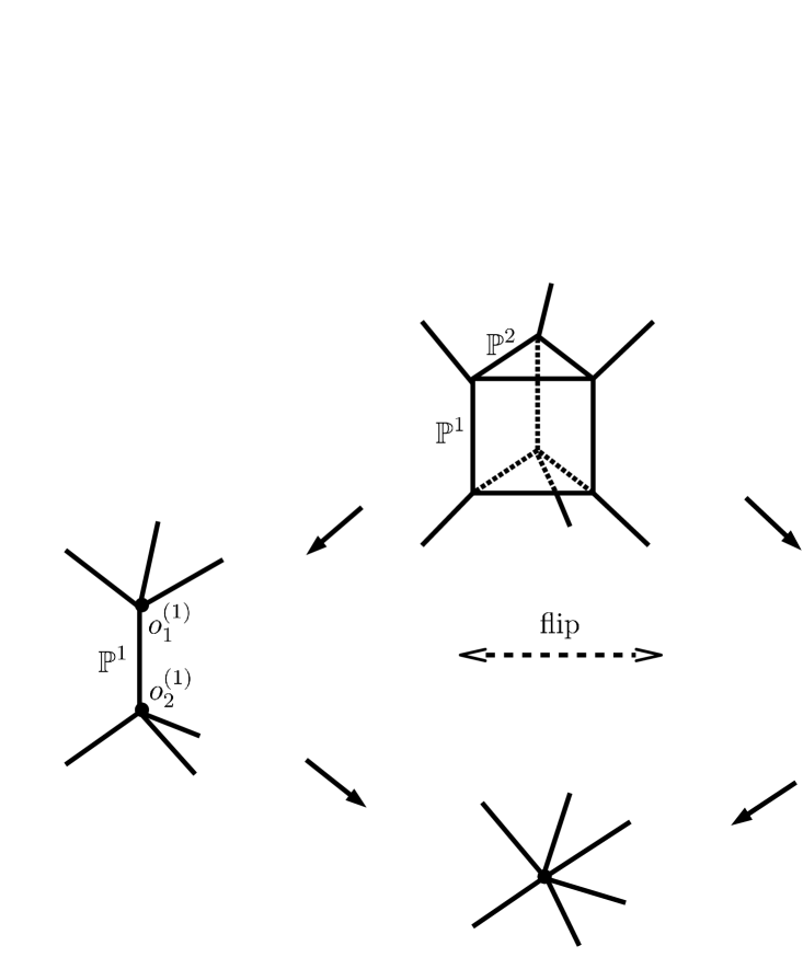
Figure 3.1. Fig.1 Four dimensional flip in the resolutions of $\mathrm{Spec}\,{\mathbb{C}}[C_{NE}\cap L]$. All boundary points $o_{i}^{(a)}$ are LCSLs.

(3.2.b) Power series solutions and Picard-Fuchs equations. In this subsection, we give the power series solutions of the GKZ $\mathcal{A}$-hypergeometric system near the LCSL in the the affine chart $\mathrm{Spec}\,\mathbb{C}[C_{NE}\cap L]$ (see Appendix A). To simplify the form of the power series, we normalize the period integral (2.1) as follows:

(3.4) $$\omega_{C}(a):=\sqrt{a_{0}b_{0}c_{0}}\;\bar{\omega}_{C}(a).$$

Definition 3.5.

Let $(\sigma_{i}^{(k)})^{\vee}$ be the dual cone of $\sigma_{i}^{(k)}$ in (3.3), which is smooth. We represent $(\sigma_{i}^{(k)})^{\vee}$ in $L_{\mathbb{R}}$ by using (B.1). Then in terms of its primitive generators, we have

$$(\sigma_{i}^{(k)})^{\vee}=\mathrm{Cone}\left\{\ell^{(1)},\ell^{(2)},\ell^{(3)},\ell^{(4)}\right\}.$$

Let $z_{m}:=\mathtt{a^{\ell^{(m)}}}=\prod_{i=1}^{9}\mathtt{a}_{i}^{\ell_{i}^{(m)}}$ be the affine coordinates on $\mathrm{Spec}\,\mathbb{C}[(\sigma_{i}^{(m)})^{\vee}\cap L]$ with arranging the parameters

$$\mathtt{a}:=(-a_{0,}-b_{0},-c_{0},a_{1},a_{2},b_{1},b_{2},c_{1},c_{2}).$$

Then the hypergeometric series associated to $\sigma_{i}^{(a)}$ is defined to be

(3.5) $$\omega_{0}(z)=\sum_{n_{1},...,n_{4}\geq 0}\frac{1}{\Gamma(\frac{1}{2})^{3}}\frac{\prod_{i=1}^{3}\Gamma(n\cdot\ell_{i}+\frac{1}{2})}{\prod_{i=4}^{9}\Gamma(n\cdot\ell_{i}+1)}z_{1}^{n_{1}}z_{2}^{n_{2}}z_{3}^{n_{3}}z_{4}^{n_{4}},$$

where $n\cdot\ell:=\sum_{k}n_{k}\ell^{(k)}$ (see [16, 17]).

The hypergeometric series $w_{0}(z)$ is the unique power series solution of the GKZ $\mathcal{A}$-hypergeometric system on $\mathcal{M}_{SecP}$ near a LCSL point. We now use the method developed in [17] to determine the complete set of the Picard-Fuchs differential operators. To show the calculations, we take the affine chart $\mathrm{Spec}\,\mathbb{C}[(\sigma_{1}^{(1)})^{\vee}\cap L]$ as an example. It should be clear that the constructions below are parallel for the other cases $\mathrm{Spec}\,\mathbb{C}[(\sigma_{i}^{(k)})^{\vee}\cap L]$.

As the primitive generator of $(\sigma_{1}^{(1)})^{\vee}\subset L_{\mathbb{R}}$, we first obtain

$$\begin{matrix}\ell^{(1)}=(-1,\;\;\,0,\;\;\,0,\;\;\,1,\;\;\,0,\;\;\,0,\;\;\,0,\;\;\,1,-1),\\ \ell^{(2)}=(\;\;\,0,-1,\;\;\,0,\;\;\,1,-1,\;\;\,1,\;\;\,0,\;\;\,0,\;\;\,0),\\ \ell^{(3)}=(\;\;\,0,\;\;\,0,-1,\;\;\,0,\;\;\,0,\;\;\,1,-1,\;\;\,1,\;\;\,0),\\ \ell^{(4)}=(\;\;\,0,\;\;\,0,\;\;\,0,-1,\;\;\,1,-1,\;\;\,1,-1,\;\;\,1).\end{matrix}$$

The power series (3.5) now becomes

(3.6) $$\omega_{0}(z)=\sum_{n_{1},n_{2},n_{3},n_{4}\geq 0}c(n_{1},n_{2},n_{3},n_{4})z_{1}^{n_{1}}z_{2}^{n_{2}}z_{3}^{n_{3}}z_{4}^{n_{4}}$$

with the coefficients $c(n)=c(n_{1},n_{2},n_{3},n_{4})$ given by

$$c(n):=\frac{1}{\Gamma(\frac{1}{2})^{3}}\frac{\Gamma(n_{1}+\frac{1}{2})\Gamma(n_{2}+\frac{1}{2})\Gamma(n_{3}+\frac{1}{2})}{\Pi_{{}_{i=1}}^{3}\Gamma(n_{4}-n_{i}+1)\cdot\Pi_{1\leq j<k\leq 3}\Gamma(n_{j}+n_{k}-n_{4}+1)}.$$

Picard-Fuchs differential equations may be characterized by the set of differential operators which annihilate the power series $\omega_{0}(z)$. In the present case, since the period integrals (normalized by $\sqrt{a_{0}b_{0}c_{0}}$) satisfy the GKZ $\mathcal{A}$-hypergeometric system we can construct them from the elements $\ell\in(\sigma_{1}^{(1)})^{\vee}\cap L$ . The method in [17] produces finite set of operators in terms of Gröbner basis.

Let $\ell=\ell_{+}-\ell_{-}$ be the unique decomposition under the conditions $\ell_{\pm}\in\mathbb{Z}_{\geq 0}^{9}$ and ${\rm supp}(\ell_{+})\cap{\rm supp}(\ell_{-})=\phi$. For such decomposition $\ell=\ell_{+}-\ell_{-}$, we define the GKZ differential operator by $\square_{\ell}=\left(\frac{\partial\;}{\partial\mathtt{a}}\right)^{\ell_{+}}-\left(\frac{\partial\;}{\partial\mathtt{a}}\right)^{\ell_{-}}$. We use the multi-degree convention $\mathtt{a}^{m}:=\Pi_{i=1}^{9}\mathtt{a}_{i}^{m_{i}}$ as above, and similarly for $\left(\frac{\partial\;}{\partial\mathtt{a}}\right)^{m}$. Following the reference [17], we define

$$\mathtt{a}^{\ell_{+}}\square_{l}=\mathtt{a}^{\ell_{+}}\left(\frac{\partial\;}{\partial\mathtt{a}}\right)^{\ell_{+}}-\mathtt{a}^{\ell}\cdot\mathtt{a}^{\ell_{-}}\left(\frac{\partial\;}{\partial\mathtt{a}}\right)^{\ell_{-}},$$

which we can express in terms of $\theta_{\mathtt{a}_{i}}:=\mathtt{a}_{i}\frac{\partial\;}{\partial\mathtt{a}_{i}}$ and a monomial of $z_{m}:=\mathtt{a}^{\ell^{(m)}}$ since $\ell\in(\sigma_{1}^{(1)})^{\vee}\cap L$ and $\ell^{(m)}$’s generate the cone. Our period integrals $\omega_{C}(a)$ are related to GKZ hypergeometric series by the factor $\sqrt{a_{0}b_{0}c_{0}}$ as in (3.4), hence the differential operators

$$\mathcal{D}_{\ell}:=(a_{0}b_{0}c_{0})^{\frac{1}{2}}\left(\mathtt{a}^{\ell_{+}}\square_{l}\right)(a_{0}b_{0}c_{0})^{-\frac{1}{2}}$$

annihilate the normalized period integrals $\omega_{C}(a).$ In Appendix C, we list a minimal set of differential operators which determine the period integrals around the origin of the affine chart $\mathrm{Spec}\,\mathbb{C}[(\sigma_{1}^{(1)})^{\vee}\cap L]$.

Proposition 3.6.

The period integral $\omega_{0}(z)$ in (3.6) is the only power series solution near a LCSL given by the origin of $\mathrm{Spec}\,\mathbb{C}[(\sigma_{1}^{(1)})^{\vee}\cap L]\simeq\mathbb{C}^{4}$. The origin is the special point (LCSL) where all other linearly independent solutions contain some powers of $\log z_{i}\;(i=1,...,4).$

Proof.

The first claim can be verified by the set of differential operators in Appendix C. For the second claim, we will find a closed formula for the logarithmic solutions. The closed formula will be described in detail in [18]. ∎

Calculations are completely parallel for all other origins $o_{i}^{(k)}$ of the affine charts $\mathrm{Spec}\,\mathbb{C}[(\sigma_{i}^{(k)})^{\vee}\cap L]$ of the resolutions. One can verify the corresponding properties in the above proposition hold for all $o_{i}^{(k)}$.

Remark 3.7.

As noted in Remark 3.2, the six singular vertices in the secondary polytope $Sec(\mathcal{A})$ come from the combinatorial symmetry when reading $\mathcal{A}$ from the period integral (3.1). Hence, up to permutations among the variables $a_{i}$, $b_{j}$ and $c_{k}$, respectively, the hypergeometric series which we define for each of the six affine chart have the same form as (3.6). Therefore the Picard-Fuchs differential operators have the same form, up to suitable conjugations by monomial factors, for all six affine charts of the form $\mathrm{Spec}\,\mathbb{C}[C_{NE}\cap L]$ from the vertices $T_{1},...,T_{6}$. Based on this simple property, we will have the same Fourier expansions for the certain lambda functions when expanded around the boundary points. Details are described in [18].

4. $\mathcal{M}_{3,3}$ from period integrals

As presented in [16, 17] for the case of Calabi-Yau complete intersections in toric varieties, GKZ hypergeometric systems provide powerful means for calculating various predictions of mirror symmetry. One may naively expects that this is also the case for $E(3,6)$. However, it turns out that we need to further understand relationships between the compactifications $\mathcal{M}_{SecP}$ , $\mathcal{M}_{3,3}$ and finally $\mathcal{M}_{6}$. In this section, we will find that the compactification$\mathcal{M}_{3,3}$ arises naturally from evaluating period integrals. We will see that $\mathcal{M}_{SecP}$ is actually a partial resolution of $\mathcal{M}_{3,3}$.

4.1. Power series from residue calculations

Recall that, when determining Picard-Fuchs differential operators in the previous section, we have normalized the period integral (2.1) by $\omega_{C}(a)=\sqrt{a_{0}b_{0}c_{0}}\;\bar{\omega}_{C}(a).$ Under this normalization, by making use of the expansion $\frac{1}{\sqrt{1+P}}=\sum r_{n}P^{n}$, we can evaluate the period integral over the torus cycle $\gamma=\left\{|{\tt x}|=|{\tt y}|=\varepsilon\right\}$ as follows

$$\begin{aligned} \int\frac{\sqrt{a_{0}b_{0}c_{0}}}{\sqrt{(a_{0}+\frac{a_{2}}{{\tt x}}+a_{1}\frac{{\tt y}}{{\tt x}})(b_{0}+\frac{b_{1}}{{\tt y}}+b_{2}\frac{{\tt x}}{{\tt y}})(c_{0}+c_{1}{\tt x}+c_{2}{\tt y})}}\frac{d{\tt x}d{\tt y}}{{\tt x}{\tt y}}\end{aligned}$$

$$=\int\sum_{n,m,k}r_{n}\left(\frac{a_{2}}{a_{0}}\frac{1}{{\tt x}}+\frac{a_{1}}{a_{0}}\frac{{\tt y}}{{\tt x}}\right)^{n}r_{m}\left(\frac{b_{1}}{b_{0}}\frac{1}{{\tt y}}+\frac{b_{2}}{b_{0}}\frac{{\tt x}}{{\tt y}}\right)^{m}r_{k}\left(\frac{c_{1}}{c_{0}}{\tt x}+\frac{c_{2}}{c_{0}}{\tt y}\right)^{k}\frac{d{\tt x}d{\tt y}}{{\tt x}{\tt y}}$$

by formally evaluating the residues.

Lemma 4.1.

We have the period integrals over the torus cycle $\gamma$ as a power series of

(4.1) $$x:=\frac{a_{2}c_{1}}{a_{0}c_{0}},y:=\frac{a_{1}b_{2}}{a_{0}b_{0}},z:=\frac{b_{1}c_{2}}{b_{0}c_{0}},u:=-\frac{a_{1}b_{1}c_{1}}{a_{0}b_{0}c_{0}},v:=-\frac{a_{2}b_{2}c_{2}}{a_{0}b_{0}c_{0}}$$

which satisfy the equation $xyz=uv$. Eliminating the powers of $v$, the result is formally expressed by

(4.2) $$\omega_{0}(x,y,z,u):=\sum_{l=-\infty}^{\infty}\sum_{\;\;\;m,n,k\geq\max\left\{0,-l\right\}}c(n,m,k,l)x^{n}y^{m}z^{k}u^{l},$$

where

$$c(n,m,k,l):=\frac{1}{\Gamma(\frac{1}{2})^{3}}\frac{\Gamma(m+n+l+\frac{1}{2})\Gamma(n+k+l+\frac{1}{2})\Gamma(m+k+l+\frac{1}{2})}{m!\,n!\,k!\,(m+l)!\,(n+l)!\,(k+l)!}.$$

Proof.

The evaluation of the residues is straightforward (cf. [3, 17]). The closed formula of the coefficients $c(n,m,k,l)$ can be deduced from the formal solutions of the GKZ system [10]. ∎

Proposition 4.2.

The Laurent series $\omega_{0}(x,y,z,u)$ defines a regular solutions around a point $[0,0,0,0,0,1]\in\mathcal{M}_{3,3}$ under the following identification of the parameters $x,y,z,u,v$ with the affine coordinate of $\mathcal{M}_{3,3}$:

$$\left\{[x,y,z,u,v,1]\in\mathbb{P}^{5}\mid xyz=1\,uv\right\}\subset\mathcal{M}_{3,3}.$$

Proof.

By the definitions of $x,y,z,u,v$, we have the relation $xyz=uv$. The claim is clear since we have a power series of $x,y,z,u,v$ in Lemma 4.1 (before eliminating $v$). ∎

Remark 4.3.

Recall that we have made a choice, among six combinatorial possibilities, from the first line to the second line of (3.1) as noted in Remark 3.2. It is easy to deduce that, if we change our choice there, we will have the same power series but with different variables, which corresponds to expansions around different coordinate points of $\mathbb{P}^{5}$ (cf. Remark 3.7). Namely, when we reduce the $GL(3,\mathbb{C})$ symmetry to the diagonal tori as in (2.7), we may consider that the period integral (3.1) is defined on

$$\mathcal{M}_{3,3}=\left\{X_{0}X_{1}X_{2}=X_{3}X_{4}X_{5}\right\}\subset\mathbb{P}^{5}.$$

4.2. $\mathcal{M}_{SecP}$ and $\mathcal{M}_{3,3}$

We have seen in Proposition 3.6 that the special boundary points (LCSLs) appear in the resolutions of $\mathcal{M}_{SecP}$ . Here it turns out that $\mathcal{M}_{SecP}$ gives a partial resolution of $\mathcal{M}_{3,3}$.

Proposition 4.4.

The toric hypersurface $\mathcal{M}_{3,3}\subset\mathbb{P}^{5}$ contains all coordinate lines of $\mathbb{P}^{5}.$ The singularities of $\mathcal{M}_{3,3}$ consist of six coordinate points $p_{i}(i=0,..,5)$ of $\mathbb{P}^{5}$ and nine coordinate lines $\overline{p_{i}p_{j}}$ $(0\leq i\leq 2,3\leq j\leq 5)$.

Proof.

Since all claims are easy to verify from the defining equation of the hypersurface, we omit the proofs. ∎

Figure 4.1. Fig.2 Singularities of ${\mathcal{M}}_{3,3}$. Solid lines represent the coordinate lines $\overline{p_{i}p_{j}}$ $(0\leq i\leq 2,3\leq j\leq 5)$ along which ${\mathcal{M}}_{3,3}$ is singular. Broken lines are the other coordinate lines contained in ${\mathcal{M}}_{3,3}$.

The following lemma is our first step to relate $\mathcal{M}_{SecP}$ and $\mathcal{M}_{3,3}$. To state it, we recall that the the secondary polytope $Sec(\mathcal{A})$ has 108 vertices, whose associated cones define coordinate rings of the affine charts of $\mathcal{M}_{SecP}$. Of the 108 vertices, the six vertices $\mathcal{V}$ given in Appendix A are singular while the rest are smooth (see Proposition 2.5).

Lemma 4.5.

We have $\mathcal{M}_{3,3}=\mathbb{P}_{Conv(\mathcal{V})}$.

Proof.

This follows from the explicit calculation of $Conv(\mathcal{A})$. We list the six vertices $\mathcal{V}$ of $Sec(\mathcal{A})$ in Appendix A. From the list, it is straightforward to see the claim. ∎

By the obvious symmetry of $\mathcal{M}_{3,3}$, we may restrict our attention to the local affine geometry

$$\mathcal{M}_{3,3}^{Loc}:=\left\{xyz=uv\right\}\subset\mathbb{C}^{5},$$

and deduce its relation to the resolution $\widetilde{\mathcal{M}}_{SecP}$. If we read the exponents of the variables in (4.1), we can write the toric singularity $\mathcal{M}_{3,3}^{Loc}$ using the lattice (2.10) as

$$\mathcal{M}_{3,3}^{Loc}=\mathrm{Spec}\,\mathbb{C}[C_{0}\cap L],$$

where

(4.3) $$C_{0}:=\mathrm{Cone}\left\{\begin{aligned} (-1,\;\;\,0,-1,0,1,0,0,1,0),\\ (-1,-1,\,\;\;0,1,0,0,1,0,0),\\ (\;\;\,0,-1,-1,0,0,1,0,0,1),\\ (-1,-1,-1,1,0,1,0,1,0),\\ (-1,-1,-1,0,1,0,1,0,1)\,\end{aligned}\right\}.$$

Note that the five generators $\ell\in L$ of $C_{0}$ listed here express the the affine coordinates $x,y,z,u,v$ in (4.1) by the monomials $\mathtt{a}^{\ell}$. Under (B.1), we can also write $C_{0}$ by

$$C_{0}=\mathrm{Cone}\left\{(0,1,0,0),(1,0,0,1),(0,0,1,0),(1,0,1,0),(0,1,0,1\}\right\}\subset\mathbb{R}^{4}.$$

Note, from the form of $C_{0}$ in (4.3) and $C_{NE}$ in Appendix A, that $C_{0}$ and $C_{NE}$ are cones from the same vertex $T_{1}$ of $Sec(\mathcal{A})$.

Lemma 4.6.

We have $C_{0}\subset C_{NE}\subset L_{\mathbb{R}}$ for the cone $C_{NE}$.

Proof.

Since the vertex is chosen in common for $C_{NE}$ and $C_{0}$, the claimed inclusion is easy to verify. ∎

In Appendix A, we have listed the primitive generators of the dual cone $C_{0}^{\vee}$, which we denote by $\mu_{1},\cdots,\mu_{6}$ in order. Similarly we write the primitive generators of the dual cone $C_{NE}^{\vee}$ by $\rho_{1},...,\rho_{5}.$ Note that, by Lemma 4.6, we have the reversed inclusion as a set for the dual cones, i.e.,

$$\mathrm{supp}\,C_{0}^{\vee}\supset\mathrm{supp\,}C_{NE}^{\vee}$$

holds for the supports, in particular, the rays generated by $\rho_{1},\cdots,\rho_{5}$ are contained in $C_{0}^{\vee}$. Recall that the dual cone $C_{NE}^{\vee}$ has two possible subdivisions into smooth simplicial cones as described in Lemma 3.3 (2). In the following lemma, we consider subdivisions of the dual cone $C_{0}^{\vee}$ using all rays generated by $\mu_{1},\cdots,\mu_{6},\rho_{1},\cdots,\rho_{5}$.

Lemma 4.7.

Up to the subdivisions of $C_{NE}^{\vee}$ in Lemma 3.3 (2), there is a unique subdivision of $C_{0}^{\vee}$ into smooth simplicial cones which contains the dual cone $C_{NE}^{\vee}$ as a simplicial subset.

Proof.

By explicit construction of all possible subdivisions, via a C++ code TOPCOM [23], we find 54 subdivisions. We verify the claimed property from them.∎

Lemma 4.8.

By the unique subdivision of $C_{0}^{\vee}$ in Lemma 4.7 which contains $C_{NE}^{\vee}$ as the simplicial subset, we have a partial resolution of the singularity $\mathcal{M}_{3,3}^{Loc}=\mathrm{Spec}\,\mathbb{C}[C_{0}\cap L]$.

Proof.

The claim is clear, since $C_{0}^{\vee}$ consists of smooth cones up to subdivisions of $C_{NE}^{\vee}$.∎

Proposition 4.9.

The partial resolutions at each singular points gives globally a partial resolution $\mathcal{M}_{SecP}\to\mathcal{M}_{3,3}.$

Proof.

Our proof is based on the explicit coordinate description of $\mathcal{M}_{SecP}$ calculating the secondary polytope. See also Remark 4.10 below.∎

Remark 4.10.

Toric resolutions of $\mathcal{M}_{SecP}$ have been described in Proposition 5.7. In the next section, we will obtain the same resolutions by blowing-up along the singular locus of $\mathcal{M}_{3,3}$ (Proposition 5.7). In Fig.4, we depict one of the two possible resolutions of $\mathcal{M}_{3,3}^{Loc}$ schematically. As we see from the picture, the resolution of the singularity is covered by 19 affine coordinate charts which correspond to 19 maximal dimensional cones in the subdivision of $C_{0}^{\vee}$. If we remove the subdivision of $C_{NE}^{\vee}\subset C_{0}^{\vee}$, then the number reduces to 18, which is explained by 17 smooth maximal cones and one singular cone $C_{NE}^{\vee}$ corresponding to $\mathrm{Spec}\,\mathbb{C}[C_{NE}\cap L]$. One can also see the claim in Proposition 4.9 in a simple counting $18\times 6=108$ (see Proposition 2.5).

5. More on the resolutions of $\mathcal{M}_{3,3}$

In this section, we will describe the resolution without recourse to the toric geometry of the secondary fan. This will allow us to relate $\mathcal{M}_{SecP}$ to the geometry of the Baily-Borel-Satake compactification $\mathcal{M}_{6}$. Recall that we have defined

$$\mathcal{M}_{3,3}^{Loc}=\mathrm{Spec}\,\mathbb{C}[C_{0}\cap L]\simeq\left\{(x,y,z,u,v)\mid xyz=uv\right\},$$

which which describes the local structure of the singularities in $\mathcal{M}_{3,3}$. We shall write $\mathcal{X}=\mathcal{M}_{3,3}^{Loc}$ for short in what follows.

5.1. Blowing-up $\mathcal{X}^{\prime}\to\mathcal{X}$ along the singular locus

From the defining equation $xyz=uv$, it is easy to see that the affine hypersurface $\mathcal{X}\subset\mathbb{C}^{5}$ is singular along the three coordinate lines of $x,y,z$ coordinates (cf. Subsection 4.2). Note that we can write the union of these lines in $\mathbb{C}^{5}$ by

$$\Gamma:=\{u=v=xy=yz=zx=0\}.$$

We will consider the blow-up $\pi_{1}\colon\mathcal{X}^{\prime}\to\mathcal{X}$ along this locus $\Gamma$. Let us first introduce the blow up $\widetilde{\mathbb{C}_{\Gamma}^{5}}\subset\mathbb{C}^{5}\times\mathbb{P}^{4}$ starting with the relations

$$u:v:yz:zx:xy=U:V:W_{1}:W_{2}:W_{3},$$

for $(u,v,x,y,z)\times[U,V,W_{1},W_{2},W_{3}]\in\mathbb{C}^{5}\times\mathbb{P}^{4}$. The ideal $I_{\widetilde{\mathbb{C}_{\Gamma}^{5}}}$ of the blow-up $\widetilde{\mathbb{C}_{\Gamma}^{5}}\subset\mathbb{C}^{5}\times\mathbb{P}^{4}$ is an irreducible component of the scheme defined by the above relations. We denote by $\pi_{0}:\widetilde{\mathbb{C}_{\Gamma}^{5}}\rightarrow\mathbb{C}^{5}$ the natural projection. Then the blow-up $\mathcal{X}^{\prime}$ is the strict transform of $\mathcal{X}\subset\mathbb{C}^{5}$ by the birational map $\pi_{0}$.

Proposition 5.1.

The blow-up $\mathcal{X}^{\prime}$ is given in $\mathbb{C}^{5}\times\mathbb{P}^{4}$ by the following equations:

(5.1) $$\begin{matrix}\begin{aligned} W_{1}W_{2}&=UVz,&&&W_{1}W_{3}&=UVy,&&&W_{2}W_{3}&=UVx,\\ W_{1}x&=Uv&&&W_{2}y&=Uv&&&W_{3}z&=Uv\\ W_{1}x&=Vu,&&&W_{2}y&=Vu,&&&W_{3}z&=Vu\end{aligned}\end{matrix}$$

and

(5.2) $$\begin{matrix}\begin{aligned} W_{1}u&=yzU,&&&W_{2}u&=zxU,&&&W_{3}u&=xyU,\\ W_{1}v&=yzV,&&&W_{2}v&=zxV,&&&W_{3}v&=xyV.\end{aligned}\end{matrix}$$

Proof.

The ideal $I_{\widetilde{\mathbb{C}_{\Gamma}^{4}}}$ and the equation $xyz=uv$ define the ideal $I_{T}$ of the total transform of $\mathcal{X}$. Calculating the primary decomposition of $I_{T}$ by Singular [5], we see that the claimed equations generate the ideal of $\mathcal{X}^{\prime}$. ∎

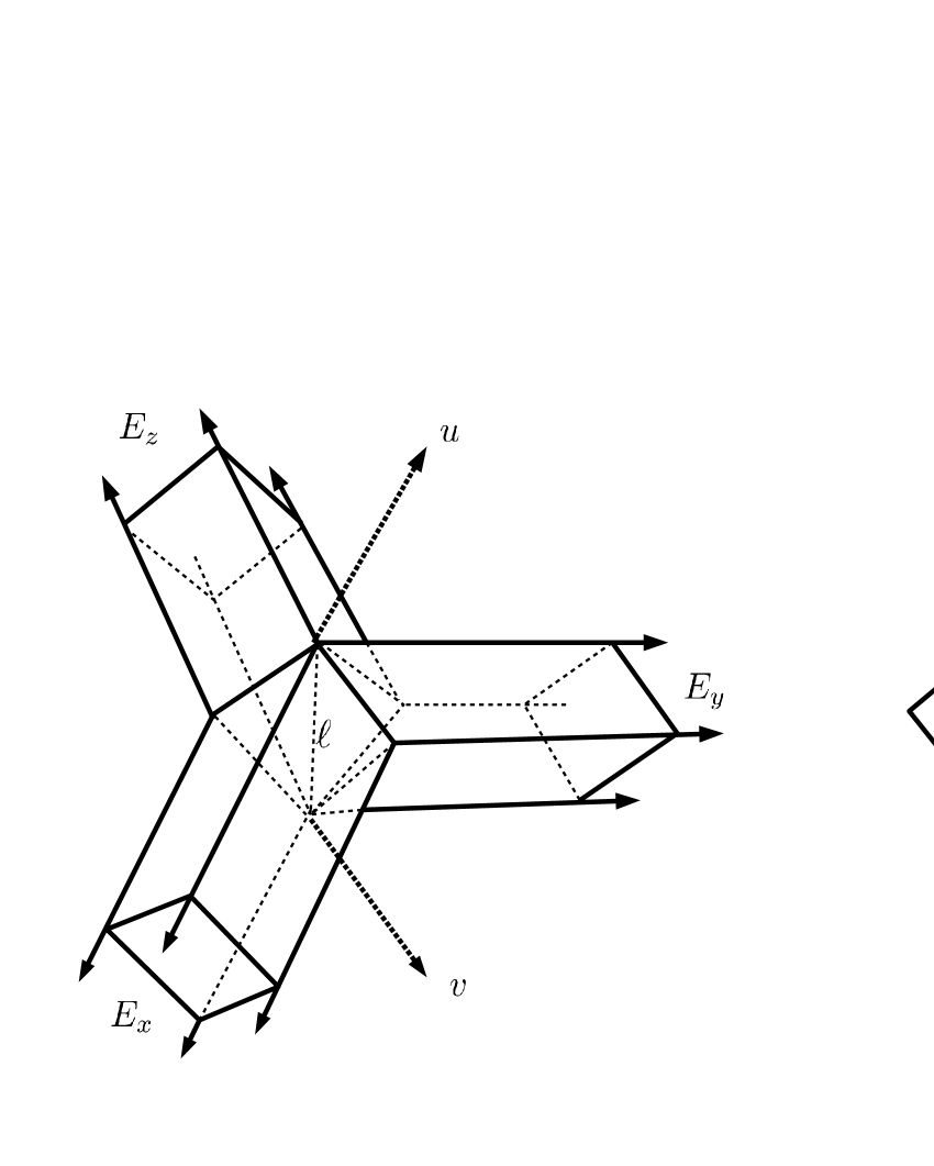
Figure 5.1. Fig.3 Exceptional divisors $E_{x},E_{y}$ and $E_{z}$ in the blow-up $\mathcal{X}^{\prime}$. Their junction locus is scaled up in the right figure.

Proposition 5.2.

The blow-up $\pi_{1}:\mathcal{X}^{\prime}\to\mathcal{X}$ has the following properties:

1. The $\pi_{1}$-exceptional divisor has three irreducible components; one for each coordinate line of $x,y,z$ coordinates. We call the irreducible components $E_{x}$, $E_{y}$, $E_{z}$, respectively.

2. The components $E_{x}$, $E_{y}$, $E_{z}$ have fibrations over the corresponding coordinate lines. The $\pi_{1}$-fiber over a point $p\in\Gamma$ is $(\mathbb{P}^{1})^{2}$ if $p$ is not the origin $o$, while over the origin it is the union of three copies $\mathbb{P}_{i}^{2}\,(i=1,2,3)$ of $\mathbb{P}^{2}$ which are glued along one line $\ell:=\mathbb{P}^{1}$ (see Fig.3). Over the origin, the components $E_{x},E_{y},E_{z}$ glue together by the following relations:

   $$E_{x}|_{\pi_{1}^{-1}(o)}=\mathbb{P}_{2}^{2}\cup\mathbb{P}_{3}^{2},\;\;E_{y}|_{\pi_{1}^{-1}(o)}=\mathbb{P}_{3}^{2}\cup\mathbb{P}_{1}^{2},\;\;E_{z}|_{\pi_{1}^{-1}(o)}=\mathbb{P}_{1}^{2}\cup\mathbb{P}_{2}^{2}.$$

3. The blow-up $\mathcal{X}^{\prime}$ is singular only at two isolated points, say, $p_{1}$ and $p_{2}$ on $\ell$. The singularities at these points are isomorphic to the affine cone over the Segre$(\mathbb{P}^{1})^{3}$.

4. The components $E_{x},E_{y}$ and $E_{z}$ are singular only at $p_{1}$ and $p_{2}$ with ODPs.

Proof.

The claimed properties follow from the equations in Proposition 5.1. For (1) and (2), because of the obvious symmetry, we only need to consider the case of $x$-axes. Set $y=z=u=v=0$ in (5.1) assuming $x\not=0$. Then we obtain $W_{1}=0$ and $W_{2}W_{3}=UVx$, from which we see $\pi_{1}^{-1}(p)\simeq\mathbb{P}^{1}\times\mathbb{P}^{1}$ $(p\not=o)$ as claimed. When $x=y=z=u=v=0$, the equations (5.1) become $W_{1}W_{2}=W_{1}W_{3}=W_{2}W_{3}=0$, from which we obtain

$$\pi_{1}^{-1}(o) =\left\{o\times[U,V,W_{1},0,0]\right\}\cup\left\{o\times[U,V,0,W_{2},0]\right\}\cup\left\{o\times[U,V,0,0,W_{3}]\right\}$$

$$=:\mathbb{P}_{1}^{2}\cup\mathbb{P}_{2}^{2}\cup\mathbb{P}_{3}^{2}.$$

Also we see that $\mathbb{P}_{1}^{2}\cap\mathbb{P}_{2}^{2}\cap\mathbb{P}_{3}^{2}=\left\{o\times[U,V,0,0,0]\right\}=:\ell$ as claimed. It is easy to see the claimed forms of $E_{x}|_{\pi_{1}^{-1}(o)},E_{y}|_{\pi_{1}^{-1}(o)}$ and $E_{x}|_{\pi_{1}^{-1}(o)}$.

To show (3), we express $\mathcal{X}^{\prime}$ in affine coordinates. By obvious symmetry, we only have to consider $\mathcal{X}^{\prime}|_{W_{1}\not=0}$ and $\mathcal{X}^{\prime}|_{U\not=0}$. Let us first describe the restriction $\mathcal{X}^{\prime}|_{W_{1}\not=0}$ by setting $W_{1}=1$. Then we obtain the relations

$$W_{2}=UVz,\;\;W_{3}=UVy,\;\;x=Vu$$

from (5.1) and also $u=Uyz,\;\;v=Vyz$ from (5.2). From these relations, we see that $\mathcal{X}^{\prime}|_{W_{1}\not=0}$ is isomorphic to $\mathbb{C}^{4}$ with the coordinates $y,z,U,V$. By symmetry, similar results hold for other cases $W_{2}\not=0$ and $W_{3}\not=0$. In particular, $\mathcal{X}^{\prime}|_{W_{i}\not=0}$ are smooth for $i=1,2,3.$

Next, let us describe $\mathcal{X}^{\prime}|_{U\not=0}$ by setting $U=1$. From (5.1), we obtain

(5.3) $$\begin{matrix}\begin{aligned} W_{1}W_{2}&=Vz,&&&W_{1}W_{3}&=Vy,&&&W_{2}W_{3}&=Vx,\\ W_{1}x&=Vu,&&&W_{2}y&=Vu,&&&W_{3}z&=Vu\end{aligned}\end{matrix}$$

in addition to $v=Vu$ which eliminates $v$. Also from (5.2), we have

(5.4) $$W_{1}u=yz, W_{2}u=zx, W_{3}u=xy$$

and also $W_{1}v=yzV,W_{2}v=zxV,W_{3}v=xyV$, where the latter three relations are consequences other relations. We note that the equations (5.3) and (5.4) are determinants of $2\times 2$ sub-matrices of the 2-hypermatrix given in the equation below. Moreover, the relations (5.3) and (5.4) are solved by $a_{ijk}$ written in terms of the homogeneous coordinates $([a_{0},a_{1}],[b_{0},b_{1}],[c_{0},c_{1}])\in(\mathbb{P}^{1})^{3}$;

$$\begin{matrix}\lx@xy@svg{\hbox{\raise 0.0pt\hbox{\kern 181.36874pt\hbox{{\hbox{\kern-102.51038pt\raise 0.0pt\hbox{\hbox{\kern 6.0pt\raise-2.57pt\hbox{$\textstyle{a_{0}b_{1}c_{1}}$}}}}}{\hbox{\kern-45.60516pt\raise 0.0pt\hbox{\hbox{\kern 6.0pt\raise-2.57pt\hbox{$\textstyle{a_{1}b_{1}c_{1}}$}}}}}{\hbox{\kern-130.96298pt\raise-28.4526pt\hbox{\hbox{\kern 6.0pt\raise-2.57pt\hbox{$\textstyle{a_{0}b_{0}c_{1}}$}}}}}{\hbox{\kern-74.05777pt\raise-28.4526pt\hbox{\hbox{\kern 6.0pt\raise-2.57pt\hbox{$\textstyle{a_{1}b_{0}c_{1}}$}}}}}{\hbox{\kern-102.51038pt\raise-56.90521pt\hbox{\hbox{\kern 6.0pt\raise-2.57pt\hbox{$\textstyle{a_{0}b_{1}c_{0}}$}}}}}{\hbox{\kern-45.60516pt\raise-56.90521pt\hbox{\hbox{\kern 6.0pt\raise-2.57pt\hbox{$\textstyle{a_{1}b_{1}c_{0}}$}}}}}{\hbox{\kern-130.96298pt\raise-85.35782pt\hbox{\hbox{\kern 6.0pt\raise-2.57pt\hbox{$\textstyle{a_{0}b_{0}c_{0}}$}}}}}{\hbox{\kern-74.05777pt\raise-85.35782pt\hbox{\hbox{\kern 6.0pt\raise-2.57pt\hbox{$\textstyle{a_{1}b_{0}c_{0}}$}}}}}{}{}{\hbox{\kern-181.36874pt\raise-42.67891pt\hbox{\hbox{\kern 0.0pt\raise-2.98334pt\hbox{$\textstyle{\big{(}a_{ijk}\big{)}\;\;=}$}}}}}{\hbox{\kern-3.8889pt\raise-42.67891pt\hbox{\hbox{\kern 0.0pt\raise-1.83438pt\hbox{$\textstyle{=}$}}}}}{\hbox{\kern 46.87744pt\raise 0.0pt\hbox{\hbox{\kern 6.0pt\raise-3.41666pt\hbox{$\textstyle{V}$}}}}}{\hbox{\kern 100.99376pt\raise 0.0pt\hbox{\hbox{\kern 6.0pt\raise-2.51443pt\hbox{$\textstyle{W_{2}}$}}}}}{\hbox{\kern 15.63594pt\raise-28.4526pt\hbox{\hbox{\kern 6.0pt\raise-2.51443pt\hbox{$\textstyle{W_{1}}$}}}}}{\hbox{\kern 76.81267pt\raise-28.4526pt\hbox{\hbox{\kern 6.0pt\raise-2.15277pt\hbox{$\textstyle{z}$}}}}}{\hbox{\kern 44.08855pt\raise-56.90521pt\hbox{\hbox{\kern 6.0pt\raise-2.51443pt\hbox{$\textstyle{W_{3}}$}}}}}{\hbox{\kern 104.95279pt\raise-56.90521pt\hbox{\hbox{\kern 6.0pt\raise-2.15277pt\hbox{$\textstyle{x}$}}}}}{\hbox{\kern 19.82181pt\raise-85.35782pt\hbox{\hbox{\kern 6.0pt\raise-1.18056pt\hbox{$\textstyle{y}$}}}}}{\hbox{\kern 76.49553pt\raise-85.35782pt\hbox{\hbox{\kern 6.0pt\raise-2.15277pt\hbox{$\textstyle{u}$}}}}}{}{}\ignorespaces\ignorespaces\ignorespaces\ignorespaces\ignorespaces{}\ignorespaces{\hbox{\lx@xy@droprule}}\ignorespaces{}\ignorespaces{\hbox{\lx@xy@droprule}}{\hbox{\lx@xy@droprule}}\ignorespaces\ignorespaces\ignorespaces\ignorespaces\ignorespaces{}\ignorespaces\ignorespaces\ignorespaces{\hbox{\lx@xy@drawline@}}\ignorespaces{}\ignorespaces\ignorespaces\ignorespaces{\hbox{\lx@xy@drawline@}}\ignorespaces{\hbox{\lx@xy@drawline@}}\ignorespaces\ignorespaces\ignorespaces\ignorespaces\ignorespaces\ignorespaces{}\ignorespaces{\hbox{\lx@xy@droprule}}\ignorespaces{}\ignorespaces{\hbox{\lx@xy@droprule}}{\hbox{\lx@xy@droprule}}\ignorespaces\ignorespaces\ignorespaces\ignorespaces\ignorespaces{}\ignorespaces\ignorespaces\ignorespaces{\hbox{\lx@xy@drawline@}}\ignorespaces{}\ignorespaces\ignorespaces\ignorespaces{\hbox{\lx@xy@drawline@}}\ignorespaces{\hbox{\lx@xy@drawline@}}\ignorespaces\ignorespaces\ignorespaces\ignorespaces\ignorespaces\ignorespaces{}\ignorespaces{\hbox{\lx@xy@droprule}}\ignorespaces{}\ignorespaces{\hbox{\lx@xy@droprule}}{\hbox{\lx@xy@droprule}}\ignorespaces\ignorespaces\ignorespaces\ignorespaces\ignorespaces\ignorespaces{}\ignorespaces{\hbox{\lx@xy@droprule}}\ignorespaces{}\ignorespaces{\hbox{\lx@xy@droprule}}{\hbox{\lx@xy@droprule}}\ignorespaces\ignorespaces\ignorespaces\ignorespaces\ignorespaces{}\ignorespaces\ignorespaces\ignorespaces{\hbox{\lx@xy@drawline@}}\ignorespaces{}\ignorespaces\ignorespaces\ignorespaces{\hbox{\lx@xy@drawline@}}\ignorespaces{\hbox{\lx@xy@drawline@}}\ignorespaces\ignorespaces\ignorespaces\ignorespaces\ignorespaces\ignorespaces{}\ignorespaces{\hbox{\lx@xy@droprule}}\ignorespaces{}\ignorespaces{\hbox{\lx@xy@droprule}}{\hbox{\lx@xy@droprule}}\ignorespaces\ignorespaces\ignorespaces\ignorespaces\ignorespaces{}\ignorespaces\ignorespaces\ignorespaces{\hbox{\lx@xy@drawline@}}\ignorespaces{}\ignorespaces\ignorespaces\ignorespaces{\hbox{\lx@xy@drawline@}}\ignorespaces{\hbox{\lx@xy@drawline@}}\ignorespaces\ignorespaces\ignorespaces\ignorespaces\ignorespaces\ignorespaces{}\ignorespaces{\hbox{\lx@xy@droprule}}\ignorespaces{}\ignorespaces{\hbox{\lx@xy@droprule}}{\hbox{\lx@xy@droprule}}\ignorespaces\ignorespaces\ignorespaces\ignorespaces\ignorespaces\ignorespaces{}\ignorespaces{\hbox{\lx@xy@droprule}}\ignorespaces{}\ignorespaces{\hbox{\lx@xy@droprule}}{\hbox{\lx@xy@droprule}}\ignorespaces\ignorespaces\ignorespaces\ignorespaces\ignorespaces\ignorespaces{}\ignorespaces{\hbox{\lx@xy@droprule}}\ignorespaces{}\ignorespaces{\hbox{\lx@xy@droprule}}{\hbox{\lx@xy@droprule}}\ignorespaces\ignorespaces\ignorespaces\ignorespaces\ignorespaces\ignorespaces{}\ignorespaces{\hbox{\lx@xy@droprule}}\ignorespaces{}\ignorespaces{\hbox{\lx@xy@droprule}}{\hbox{\lx@xy@droprule}}\ignorespaces\ignorespaces\ignorespaces\ignorespaces\ignorespaces\ignorespaces{}\ignorespaces{\hbox{\lx@xy@droprule}}\ignorespaces{}\ignorespaces{\hbox{\lx@xy@droprule}}{\hbox{\lx@xy@droprule}}\ignorespaces\ignorespaces\ignorespaces\ignorespaces\ignorespaces\ignorespaces{}\ignorespaces{\hbox{\lx@xy@droprule}}\ignorespaces{}\ignorespaces{\hbox{\lx@xy@droprule}}{\hbox{\lx@xy@droprule}}\ignorespaces\ignorespaces\ignorespaces\ignorespaces\ignorespaces{}\ignorespaces\ignorespaces\ignorespaces{\hbox{\lx@xy@drawline@}}\ignorespaces{}\ignorespaces\ignorespaces\ignorespaces{\hbox{\lx@xy@drawline@}}\ignorespaces{\hbox{\lx@xy@drawline@}}\ignorespaces\ignorespaces\ignorespaces\ignorespaces\ignorespaces\ignorespaces{}\ignorespaces{\hbox{\lx@xy@droprule}}\ignorespaces{}\ignorespaces{\hbox{\lx@xy@droprule}}{\hbox{\lx@xy@droprule}}\ignorespaces\ignorespaces\ignorespaces\ignorespaces\ignorespaces{}\ignorespaces\ignorespaces\ignorespaces{\hbox{\lx@xy@drawline@}}\ignorespaces{}\ignorespaces\ignorespaces\ignorespaces{\hbox{\lx@xy@drawline@}}\ignorespaces{\hbox{\lx@xy@drawline@}}\ignorespaces\ignorespaces\ignorespaces\ignorespaces\ignorespaces\ignorespaces{}\ignorespaces{\hbox{\lx@xy@droprule}}\ignorespaces{}\ignorespaces{\hbox{\lx@xy@droprule}}{\hbox{\lx@xy@droprule}}\ignorespaces\ignorespaces\ignorespaces\ignorespaces\ignorespaces\ignorespaces{}\ignorespaces{\hbox{\lx@xy@droprule}}\ignorespaces{}\ignorespaces{\hbox{\lx@xy@droprule}}{\hbox{\lx@xy@droprule}}\ignorespaces\ignorespaces\ignorespaces\ignorespaces\ignorespaces{}\ignorespaces\ignorespaces\ignorespaces{\hbox{\lx@xy@drawline@}}\ignorespaces{}\ignorespaces\ignorespaces\ignorespaces{\hbox{\lx@xy@drawline@}}\ignorespaces{\hbox{\lx@xy@drawline@}}\ignorespaces\ignorespaces\ignorespaces\ignorespaces\ignorespaces\ignorespaces{}\ignorespaces{\hbox{\lx@xy@droprule}}\ignorespaces{}\ignorespaces{\hbox{\lx@xy@droprule}}{\hbox{\lx@xy@droprule}}\ignorespaces\ignorespaces\ignorespaces\ignorespaces\ignorespaces{}\ignorespaces\ignorespaces\ignorespaces{\hbox{\lx@xy@drawline@}}\ignorespaces{}\ignorespaces\ignorespaces\ignorespaces{\hbox{\lx@xy@drawline@}}\ignorespaces{\hbox{\lx@xy@drawline@}}\ignorespaces\ignorespaces\ignorespaces\ignorespaces\ignorespaces\ignorespaces{}\ignorespaces{\hbox{\lx@xy@droprule}}\ignorespaces{}\ignorespaces{\hbox{\lx@xy@droprule}}{\hbox{\lx@xy@droprule}}\ignorespaces\ignorespaces\ignorespaces\ignorespaces\ignorespaces\ignorespaces{}\ignorespaces{\hbox{\lx@xy@droprule}}\ignorespaces{}\ignorespaces{\hbox{\lx@xy@droprule}}{\hbox{\lx@xy@droprule}}\ignorespaces\ignorespaces\ignorespaces\ignorespaces\ignorespaces\ignorespaces{}\ignorespaces{\hbox{\lx@xy@droprule}}\ignorespaces{}\ignorespaces{\hbox{\lx@xy@droprule}}{\hbox{\lx@xy@droprule}}\ignorespaces\ignorespaces\ignorespaces\ignorespaces\ignorespaces\ignorespaces{}\ignorespaces{\hbox{\lx@xy@droprule}}\ignorespaces{}\ignorespaces{\hbox{\lx@xy@droprule}}{\hbox{\lx@xy@droprule}}\ignorespaces\ignorespaces\ignorespaces\ignorespaces\ignorespaces\ignorespaces{}\ignorespaces{\hbox{\lx@xy@droprule}}\ignorespaces{}\ignorespaces{\hbox{\lx@xy@droprule}}{\hbox{\lx@xy@droprule}}\ignorespaces}}}}\end{matrix} \textstyle{a_{0}b_{1}c_{1}} \textstyle{a_{1}b_{1}c_{1}} \textstyle{a_{0}b_{0}c_{1}} \textstyle{a_{1}b_{0}c_{1}} \textstyle{a_{0}b_{1}c_{0}} \textstyle{a_{1}b_{1}c_{0}} \textstyle{a_{0}b_{0}c_{0}} \textstyle{a_{1}b_{0}c_{0}} \textstyle{\big{(}a_{ijk}\big{)}\;\;=} \textstyle{=} \textstyle{V} \textstyle{W_{2}} \textstyle{W_{1}} \textstyle{z} \textstyle{W_{3}} \textstyle{x} \textstyle{y} \textstyle{u} \textstyle{a_{0}b_{1}c_{1}} \textstyle{a_{1}b_{1}c_{1}} \textstyle{a_{0}b_{0}c_{1}} \textstyle{a_{1}b_{0}c_{1}} \textstyle{a_{0}b_{1}c_{0}} \textstyle{a_{1}b_{1}c_{0}} \textstyle{a_{0}b_{0}c_{0}} \textstyle{a_{1}b_{0}c_{0}} \textstyle{\big{(}a_{ijk}\big{)}\;\;=} \textstyle{=} \textstyle{V} \textstyle{W_{2}} \textstyle{W_{1}} \textstyle{z} \textstyle{W_{3}} \textstyle{x} \textstyle{y} \textstyle{u}$$

Thus we see that the relations (5.3) and (5.4) define the affine cone of the Segre$(\mathbb{P}^{1})^{3}$ in $\mathbb{C}^{8}$ with the affine coordinates $x,y,z,u,V,W_{1},W_{2},W_{3}$, which is singular at the vertex (the origin of $\mathbb{C}^{8}$). Note that the vertex corresponds to the point $p_{1}:=o\times[1,0,0,0,0]\in\mathcal{X}^{\prime}$ which is on the line $\ell=\left\{o\times[U,V,0,0,0]\right\}$. By symmetry, the other case $\mathcal{X}^{\prime}|_{V\not=0}$ can be described similarly with the vertex $p_{2}:=o\times[0,1,0,0,0]$ on the line $\ell$.

The claim (4) follows from the proof for (3). For example, we set $y=z=u=v=0$ in the equations (5.3) and (5.4). Then we can verify the claimed property for $E_{x}$. ∎

Note that $p_{1}$ and $p_{2}$ are the only singular points of $\mathcal{X}^{\prime}$. Let $\pi_{2}:\widetilde{\mathcal{X}}\to\mathcal{X}^{\prime}$ be the blow-up at $p_{1}$ and $p_{2}$. We denote by $\widetilde{E}_{x}$, $\widetilde{E}_{y}$, $\widetilde{E}_{z}$ the strict transforms of the $\pi_{1}$-exceptional divisors $E_{x}$, $E_{y}$, $E_{z}$ respectively.

Proposition 5.3.

The blow-up $\pi_{2}:\widetilde{\mathcal{X}}\to\mathcal{X}^{\prime}$ introduces exceptional divisors $D_{p_{1}},D_{p_{2}}$ which are isomorphic to $(\mathbb{P}^{1})^{3}$. The resulting composite of the blow-ups of $\mathcal{X}$ gives a resolution of singularities $\pi_{1}\circ\pi_{2}:\widetilde{\mathcal{X}}\to\mathcal{X}$. Moreover, the union $\widetilde{E}_{x}\cup\widetilde{E}_{y}\cup\widetilde{E}_{z}\cup D_{p_{1}}\cup D_{p_{2}}$ is a simple normal crossing divisor.

Proof.

The first two claims follow from Proposition 5.2. The last assertion also follows from the explicit computations. ∎

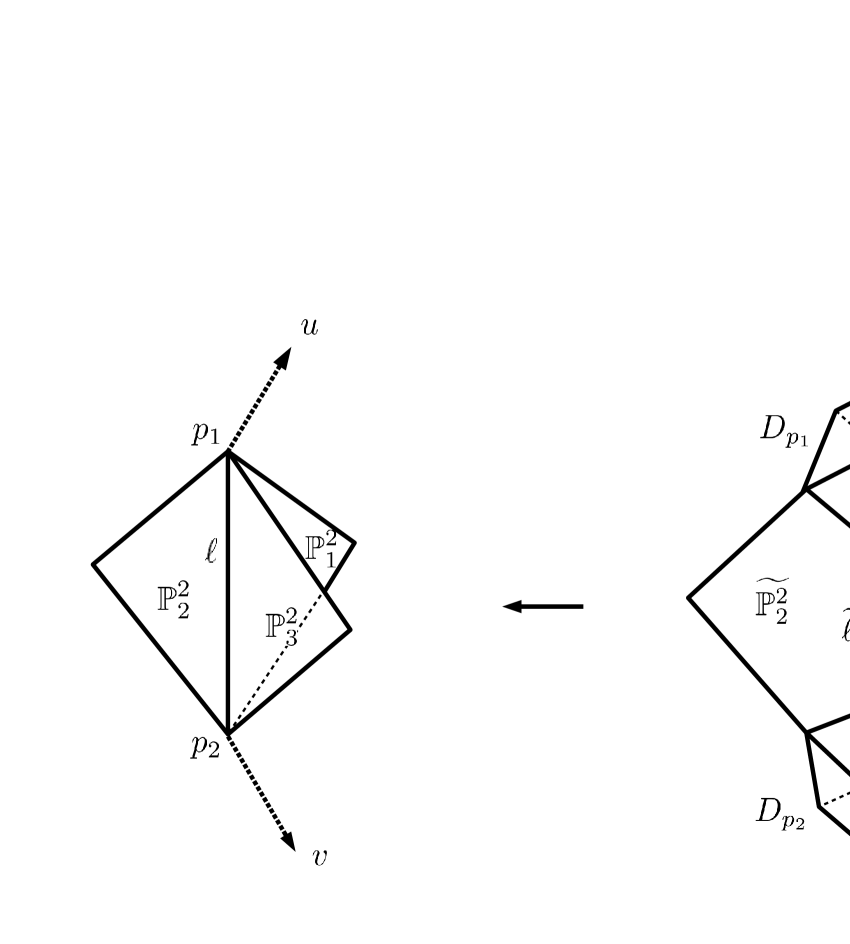
Figure 5.2. Fig.4 The blow-up of $\mathcal{X}^{\prime}$ at $p_{1}$, $p_{2}$ in the junction. The intersection points $o^{(1)}_{k}=\widetilde{E_{x}}\cap\widetilde{E_{y}}\cap\widetilde{E_{z}}\cap D_{p_{k}}$ $(k=1,2)$ and $\widetilde{\ell}$ can be identified in the left of Fig.1.

Remark 5.4.

As shown in Fig.4, the strict transforms of the three $\mathbb{P}_{i}^{2}\,(i=1,2,3)$ under the blow-up $\pi_{2}:\widetilde{\mathcal{X}}\to\mathcal{X}^{\prime}$ are $\mathbb{P}^{2}$ blown up at two points.

Making the blow-up $\widetilde{\mathcal{X}}\to\mathcal{X}=\mathcal{M}_{3,3}^{Loc}$ at each singular points of $\mathcal{M}_{3,3}$, we obtain the resolution $\widetilde{\mathcal{M}}_{SecP}$ of the partial resolution $\mathcal{M}_{SecP}\to\mathcal{M}_{3,3}$ in Proposition 3.4. Note that, in the resolution $\widetilde{\mathcal{M}}_{SecP}$ thus obtained, we have the resolution $\widetilde{\mathcal{X}}$ (the left in Fig.1) at all six singular points.

5.2. Flipping the line $\ell$ in $\widetilde{\mathcal{X}}$ to $\mathbb{P}^{2}$

Recall that we have introduced the line $\ell=\mathbb{P}_{1}^{2}\cap\mathbb{P}_{2}^{2}\cap\mathbb{P}_{3}^{2}$ in $\mathcal{X}$. Correspondingly, we have $\widetilde{\ell}=\widetilde{\mathbb{P}}_{1}^{2}\cap\widetilde{\mathbb{P}}_{2}^{2}\cap\widetilde{\mathbb{P}}_{3}^{2}$ on $\widetilde{\mathcal{X}}$. Here and in what follows we put $\widetilde{\,\,\,\,}$ to indicate the the strict transform of a subvariety of $\mathcal{X}^{\prime}$. We can also write $\ell=E_{x}\cap E_{y}\cap E_{z}$ and $\widetilde{\ell}=\widetilde{E}_{x}\cap\widetilde{E}_{y}\cap\widetilde{E}_{z}$ by Proposition 5.2. Let $N_{\widetilde{\ell}/\widetilde{\mathcal{X}}}$ be the normal bundle of $\widetilde{\ell}$ in $\widetilde{\mathcal{X}}$.

Lemma 5.5.

We have $N_{\widetilde{\ell}/\widetilde{\mathcal{X}}}\simeq\mathcal{O}_{\mathbb{P}^{1}}(-1)^{\oplus 3}$.

Proof.

By Proposition 5.3, $\widetilde{E}_{x}$, $\widetilde{E}_{y}$ and $\widetilde{E}_{z}$ are smooth on $\widetilde{\mathcal{X}}$. Since $\widetilde{\ell}=\widetilde{E}_{x}\cap\widetilde{E}_{y}\cap\widetilde{E}_{z}$, we have only to show that $\widetilde{E}_{x}\cdot\widetilde{\ell}=\widetilde{E}_{y}\cdot\widetilde{\ell}=\widetilde{E}_{z}\cdot\widetilde{\ell}=-1$. By symmetry, it suffices to show that $\widetilde{E}_{x}\cdot\widetilde{\ell}=-1$. Since $\widetilde{E}_{x}\cap\widetilde{E}_{y}=\widetilde{\mathbb{P}}_{2}^{2}$ and $\widetilde{\mathbb{P}}_{2}^{2}\cap\widetilde{\mathbb{P}}_{3}^{2}=\widetilde{\ell}$, we have $\widetilde{E}_{x}\cdot\widetilde{\ell}=(\widetilde{\mathbb{P}}_{2}^{2}\cdot\widetilde{\ell})_{\widetilde{E}_{y}}=(\widetilde{\ell}^{2})_{\widetilde{\mathbb{P}}_{3}^{2}}$. Note that $\widetilde{\mathbb{P}}_{i}^{2}\,(i=1,2,3)$ is a $\mathbb{P}^{2}$ blown-up at two points and $\widetilde{\ell}$ is a $(-1)$-curve on $\widetilde{\mathbb{P}}_{i}^{2}$. Therefore $(\widetilde{\ell}^{2})_{\widetilde{\mathbb{P}}_{3}^{2}}=-1$ as claimed. ∎

Proposition 5.6.

There is a flip which transforms the line $\widetilde{\ell}$ to $\mathbb{P}^{2}.$

Proof.

Here we only consider analytically for simplicity. See the proof of Theorem 6.12 for an algebraic construction of the flip. Since $N_{\widetilde{\ell}/\widetilde{\mathcal{X}}}\simeq\mathcal{O}_{\mathbb{P}^{1}}(-1)^{\oplus 3}$, by blowing-up along the line $\ell$, we obtain $\ell\times\mathbb{P}^{2}$ as the exceptional divisor. Contracting this to $\mathbb{P}^{2}$, we obtain the flip (cf. Fig.1). ∎

We denote by $\widetilde{\mathcal{X}}^{+}\to\mathcal{X}$ the resulting resolution after the flip of the resolution $\widetilde{\mathcal{X}}\to\mathcal{X}=\mathcal{M}_{3,3}^{Loc}$.

Proposition 5.7.

Making resolutions $\widetilde{\mathcal{X}}\to\mathcal{X}$ or $\widetilde{\mathcal{X}}^{+}\to\mathcal{X}$ locally at each of six isomorphic singular points of $\mathcal{M}_{3,3}$, we obtain the same resolution as the toric resolutions of $\mathcal{M}_{3,3}$ in Proposition 4.9 and Proposition 3.4.

Proof.

We verify the claim explicitly by writing the resolutions of $\mathcal{M}_{SecP}$ in Proposition 3.4. Here we only sketch our calculations. As described in the proof of Proposition 3.4, the partial resolution $\mathcal{M}_{SecP}$ of $\mathcal{M}_{3,3}$ is covered by 108 affine charts, among which six charts are singular. The singular charts are isomorphic to $\mathrm{Spec}\,\mathbb{C}[C_{NE}\cap L]$ which has two resolutions shown in Fig.1. By explicit calculations, we find that 108 affine charts are grouped into six isomorphic blocks of 18 charts (one singular and 17 smooth charts). We verify that each block is isomorphic to $\widetilde{\mathcal{X}}$ or $\widetilde{\mathcal{X}}^{+}$ after making a resolution of the singular chart. ∎

The above proposition provides us a global picture of the parameter space of the GKZ $\mathcal{A}$-hypergeometric system in Proposition 3.1. Our task in the next section is to make a covering of the parameter space $E(3,6)$ by certain Zariski open subsets of the parameter space of the GKZ $\mathcal{A}$-hypergeometric system.

Remark 5.8.

Instead of constructing the resolution $\widetilde{\mathcal{X}}\to\mathcal{X}$ starting with the blow-up $\mathcal{X}^{\prime}$ along $\Gamma$, we can also make a resolution by first blowing-up along $z$-coordinate line and then blowing-up along $x$- and $y$-coordinate lines. Since the (strict transforms of) $x$- and $y$-coordinate lines are separated by the first blowing-up along $z$-coordinate line, and the singularities along these lines are of $A_{1}$ type, we obtain a resolution $\widehat{\mathcal{X}}\to\mathcal{X}$ in this way. Note that the resolution $\widehat{\mathcal{X}}\to\mathcal{X}$ introduces only three exceptional divisors from the blowing-ups, and hence this is not isomorphic to $\widetilde{\mathcal{X}}\to\mathcal{X}$ in Proposition 5.3 nor $\widetilde{\mathcal{X}}^{+}\to\mathcal{X}$. Moreover, the generalized Frobenius method developed in [17, 16] does not apply to the resolution $\widehat{\mathcal{X}}\to\mathcal{X}$. Recall that the generalized Frobenius method provides a closed formula for the local solutions around special boundary points (LCSLs), such as $o_{i}^{(k)}$ in $\widetilde{\mathcal{X}}\to\mathcal{X}$ or $\widetilde{\mathcal{X}}^{+}\to\mathcal{X}$, given by normal crossing boundary or exceptional divisors. In the resolution $\widehat{\mathcal{X}}\to\mathcal{X}$, there is no way to have such special boundary points by the three exceptional divisors.

6. Blowing-up the Baily-Borel-Satake compactification $\mathcal{M}_{6}$

We will study the relationship between the Baily-Borel-Satake compactification $\mathcal{M}_{6}$ and the compactification $\mathcal{M}_{3,3}$, which appears naturally from computing the period integrals. We recall that the compactification $\mathcal{M}_{6}$ is birational to $\mathcal{M}_{3,3}$ with the birational map given by (2.6).

6.1. Birational map $\phi:\mathcal{M}_{3,3}\dashrightarrow\mathcal{M}_{6}$

Since both $\mathcal{M}_{6}$ and $\mathcal{M}_{3,3}$ have descriptions in term of GIT quotients, the birational map $\phi$ can be given explicitly by writing the relevant semi-invariants [6, 24]. We have sketched the results in Appendix K3 surfaces from configurations of six lines in $\mathbb{P}^{2}$ and mirror symmetry I; in particular, we have given the explicit form of the birational map using the (weighted-)homogeneous coordinates $[X_{0},X_{1},...,X_{5}]\in\mathbb{P}^{5}$ for $\mathcal{M}_{3,3}$ and $[Y_{0},...,Y_{4},Y_{5}]\in\mathbb{P}(1^{5},2)$ for $\mathcal{M}_{6}$.

Lemma 6.1.

The following properties holds:

1. $\phi$ defines a map $\phi:\mathcal{M}_{3,3}\setminus\left\{[1,1,1,1,1]\right\}\to\mathcal{M}_{6}$, and

2. $\phi^{-1}$ defines a map $\phi^{-1}:\mathcal{M}_{6}\setminus\left\{Y_{0}=0\right\}\to\mathcal{M}_{3,3}$.

Proposition 6.2.

Define the following divisor in $\mathcal{M}_{3,3}$:

(6.1) $$D_{0}=\left\{X_{0}+X_{1}+X_{2}-X_{3}-X_{4}-X_{5}=0\right\}.$$

Then the birational map $\phi$ restricts to a 1 to 1 map

(6.2) $$\phi:\mathcal{M}_{3,3}\setminus D_{0}\to\phi(\mathcal{M}_{3,3}\setminus D_{0})\subset\mathcal{M}_{6}$$

to its image in $\mathcal{M}_{6}$.

The proofs of the above lemma and proposition are easy from the explicit forms (C.4) and (C.5) of the birational maps $\phi$ and $\phi^{-1}$, respectively. Further properties, e.g., the restriction $\phi:D_{0}\setminus\left\{[1,1,1,1,1]\right\}\to\mathcal{M}_{6}$, can be worked out, but we leave these to the reader (see [24, Sect.2.4]).

6.2. Singularities of $\mathcal{M}_{6}$

Singularities of $\mathcal{M}_{6}$ are well-studied objects in the literatures (see [22, 19] for example). Here we summarize the results from our viewpoints and using the (weighted-)homogeneous coordinate $[Y_{0},Y_{1},...,Y_{5}]$ of $\mathbb{P}(1^{5},2)$.

Proposition 6.3.

The variety $\mathcal{M}_{6}$ is singular along 15 lines which intersect at 15 points which, respectively, correspond to one dimensional boundary components and zero dimensional boundary components in the Baily-Borel-Satake compactification. These 15 lines are located in $\left\{Y_{5}=0\right\}\simeq\mathbb{P}^{4}\subset\mathbb{P}(1^{5},2)$.

Proof.

The results are well-known in the literatures (see [28, 19] for example). An explicit description of the boundary components is given in Appendix D. ∎

Proposition 6.4.

Each of the 15 points of singularities is given by the intersection of corresponding three lines. Vice versa, each of the 15 lines contains three intersection points with other two lines at each intersection.

Proof.

We verify the claimed properties using the equations for the 15 lines in Appendix D and schematic description of the 15 lines in Fig.5. ∎

Figure 6.1. Fig.5 Configuration of the 15 lines. $\phi(p_{k})$ represent the images of the coordinate points $p_{k}$ in ${\mathcal{M}}_{3,3}$. Lines $L_{k}(k=1,...,15)$ are given explicitly in Appendix D. $L_{1},...,L_{9}$ shown in the left correspond to the 9 singular lines in ${\mathcal{M}}_{3,3}$. Lines $L_{10},...,L_{15}$ are in the divisor $\{Y_{0}=0\}$ where $\phi^{-1}$ is not defined, and intersect with $L_{1},...,L_{9}$ at one point as shown in the right.

Proposition 6.5.

The 9 lines of singularities in $\mathcal{M}_{3,3}$ described in Proposition 4.4 correspond to 9 of 15 lines in $\mathcal{M}_{6}$ by the birational map $\phi:\mathcal{M}_{3,3}\dashrightarrow\mathcal{M}_{6}$. In particular, the local structure $\mathcal{M}_{3,3}^{Loc}$ near the 6 point is isomorphically mapped to the corresponding intersection points of lines in $\mathcal{M}_{6}$.

Proof.

Recall that the 9 lines in $\mathcal{M}_{6}$ come from coordinate lines of $\mathbb{P}^{5}$ and intersect at 6 coordinate points. None of the 9 lines nor their intersection points are contained in $D_{0}$ (6.1). Hence these lines determine the corresponding lines in $\mathcal{M}_{6}$ under the birational map $\phi$, along which $\mathcal{M}_{6}$ is singular. Also the local structure $\mathcal{M}_{3,3}^{Loc}$ is mapped isomorphically to $\mathcal{M}_{6}$. ∎

In the next subsection, we will see that the local structure near all the 15 singular points in $\mathcal{M}_{6}$ are isomorphic to $\mathcal{M}_{3,3}^{Loc}$.

6.3. $S_{6}$ action on $\mathcal{M}_{6}$

Now recall that the homogeneous coordinate $Y_{i}$ is related to the $3\times 6$ matrix $A$ by (C.1). We note that there is a natural action of the symmetric group $S_{6}$ sending $A\to A\sigma:=A\rho(\sigma)$ by the permutation matrix $\rho(\sigma)$ representing $\sigma\in S_{6}$. This naturally induces linear actions on homogeneous coordinates $Y_{i}(A)\mapsto Y_{i}(A\sigma)$.

Lemma 6.6.

The action $Y_{i}=Y_{i}(A)\mapsto Y_{i}(A\sigma)$ is linear and preserves the homogeneous weights of the coordinate $[Y_{0},...,Y_{4},Y_{5}]\in\mathbb{P}(1^{5},2)$.

Proof.

The claim is clear since $Y_{i}=Y_{i}(A)$ are generators of the semi-invariants of $GL(3,\mathbb{C})$ of fixed degrees, and $Y_{i}(A\sigma)$ are semi-invariants of the same degree with $Y_{i}(A)$. ∎

Geometric meaning of the action $A\to A\sigma$ is simply that it changes the order of the (ordered) six points in $\mathbb{P}^{2}$. From Lemma 6.6, it is easy to deduce the following proposition.

Proposition 6.7.

The linear action $Y_{i}=Y_{i}(A)\mapsto Y_{i}(A\sigma)$ naturally defines the corresponding automorphism $\psi(\sigma):\mathcal{M}_{6}\simeq\mathcal{M}_{6}$ for $\sigma\in S_{6}$.

We combine this isomorphism with the birational map $\phi$: $\mathcal{M}_{3,3}\dashrightarrow\mathcal{M}_{6}$.

Definition 6.8.

For $\sigma\in S_{6}$, we define the following composite of $\psi(\sigma$) and $\phi$:

$$\phi_{\sigma}:\mathcal{M}_{3,3}\dashrightarrow\mathcal{M}_{6}\overset{\psi(\sigma)}{\simeq}\mathcal{M}_{6}.$$

6.4. Covering $\mathcal{M}_{6}$ by open sets of toric varieties

We now combine all the results about the moduli spaces $\mathcal{M}_{3,3}$ and $\mathcal{M}_{6}$. We first recall that $\mathcal{M}_{6}$ is given by a hypersurface in $\mathbb{P}(1^{5},2)$.

Lemma 6.9.

The hypersurface $\mathcal{M}_{6}$ misses the point $[0,0,0,0,0,1]\in\mathbb{P}(1^{5},2)$.

Proof.

We simply verify the property from the definition (2.4).∎

Lemma 6.10.

Take the following permutations $\sigma\in S_{6}$

$$e,(34),(35),(24),(25)$$

and name these by $\sigma_{k}\,(k=0,1,...,4)$ in order. Then under the automorphism $\psi(\sigma_{k}):\mathcal{M}_{6}\simeq\mathcal{M}_{6}$, the hyperplane $\left\{Y_{0}=0\right\}\subset\mathcal{M}_{6}$ transforms to $\left\{Y_{k}=0\right\}\subset\mathcal{M}_{6}$ for $k=0,1,...,4$, respectively.

Proof.

By lemma 6.6, $Y(A\sigma_{k})$ is linear in $Y_{i}$’s. We derive the claimed results by calculating the semi-invariants given in (C.1) under the permutations.∎

Proposition 6.11.

The moduli space $\mathbb{\mathcal{M}}_{6}$ is covered by copies of $\mathcal{M}_{3,3}\setminus D_{0}$. More precisely, we have

$$\mathcal{M}_{6}=\bigcup_{k=0}^{4}\phi_{\sigma_{k}}\left(\mathcal{M}_{3,3}\setminus D_{0}\right).$$

Proof.

By Lemma 6.9, one of the homogeneous coordinate $Y_{0},...,Y_{4}$ does not vanish for any point of $\mathcal{M}_{6}$. Then, due to Lemma 6.10, any point is contained in the union of the isomorphic images $\phi_{\sigma_{k}}\left(\mathcal{M}_{3,3}\setminus D_{0}\right)$ of $\mathcal{M}_{3,3}\setminus D_{0}$ (see (6.2) and Definition 6.8). ∎

The local structures near each of the 15 singular points in $\mathcal{M}_{6}$ is isomorphic to the local structure of $\mathcal{M}_{3,3}^{Loc}$. Making the resolution $\widetilde{\mathcal{X}}\to\mathcal{X}=\mathcal{M}_{3,3}^{Loc}$ given in Proposition 5.3 at each singular point, we have the resolution $\widetilde{\mathcal{M}}_{6}\to\mathcal{M}_{6}$. Namely, let $f_{1}\colon\mathcal{M}^{\prime}_{6}\to\mathcal{M}_{6}$ be the blow-up along $\mathrm{Sing}\,\mathcal{M}_{6}$, which is the union of $15$ lines. Then, $\mathcal{M}^{\prime}_{6}$ has $2\times 15$ singular points. Let $f_{2}\colon\widetilde{\mathcal{M}}_{6}\to\mathcal{M}^{\prime}_{6}$ be the blow-up at all the singular points.

Recall that locally we have another resolution $\widetilde{\mathcal{X}}^{+}$. In the following theorem, we can globalize this to another resolution of $\mathcal{M}_{6}$ connected with $\widetilde{\mathcal{M}}_{6}$ by a $4$-dimensional flip.

Theorem 6.12.

There exists another resolution $\widetilde{\mathcal{M}}_{6}^{+}$ of $\mathcal{M}_{6}$ which is connected with $\widetilde{\mathcal{M}}_{6}$ by a $4$-dimensional flip.

Proof.

We have already constructed the flip $\widetilde{\mathcal{X}}\dashrightarrow\widetilde{\mathcal{X}}^{+}$ of $\widetilde{\ell}$ locally analytically in Proposition 5.6. Let $\widetilde{\ell}_{1},\dots,\widetilde{\ell}_{15}\subset\widetilde{\mathcal{M}}_{6}$ be the copies of $\mathbb{P}^{1}$ over the fifteen singular points of $\mathcal{M}_{6}$. The remaining problem is to construct the flips of $\widetilde{\ell}_{1},\dots,\widetilde{\ell}_{15}$ algebraically and globally. The following properties guarantee this. We will prove them in Appendix E.

Let $E$ be the $f_{1}$-exceptional divisor and $\widetilde{E}$ its strict transform on $\widetilde{\mathcal{M}}_{6}$. Set $f:=f_{1}\circ f_{2}$. Then

1. $-(K_{\widetilde{\mathcal{M}}_{6}}+1/3\widetilde{E})$ is $f$-nef, and is numerically $f$-trivial only for $\widetilde{\ell}_{1},\dots,\widetilde{\ell}_{15}$.

2. There exists a small contraction $\rho\colon\widetilde{\mathcal{M}}_{6}\to\overline{\mathcal{M}}_{6}$ over $\mathcal{M}_{6}$ contracting exactly $\widetilde{\ell}_{1}\cup\cdots\cup\widetilde{\ell}_{15}$.

3. The contraction $\rho$ is a log flipping contraction with respect to some klt pair $(\widetilde{\mathcal{M}}_{6},D)$.

4. The flip $\widetilde{\mathcal{M}}_{6}\dashrightarrow\widetilde{\mathcal{M}}_{6}^{+}$ of $\rho$ exists and it coincides locally with the flip constructed as in Proposition 5.6.

This completes the construction of the resolution. ∎

Remark 6.13.

By Theorem 6.12, we have two algebraic resolutions $\widetilde{\mathcal{M}}_{6}\to\mathcal{M}_{6}$ and $\widetilde{\mathcal{M}}_{6}^{+}\to\mathcal{M}_{6}$, which are related by a four dimensional flip. Interestingly, it will turn out in [18] that these two possibilities of algebraic resolutions result in two non-isomorphic definitions of the lambda functions $\lambda_{K3}$ on $\mathcal{M}_{6}$.

7. Hypergeometric $\mathcal{D}$-modules on Grassmannians

In this section, we combine the results of earlier sections to give our main results of this paper.

We have obtained a global picture for the moduli space $\mathcal{M}_{6}$ in terms of the toric variety $\mathcal{M}_{3,3}$ which is closely related to the toric variety $\mathcal{M}_{SecP}$. With these results in hand, we now look at the hypergeometric system $E(3,6)$ defined on its parameter space $\mathcal{M}_{6}$. To have a global picture, it is better think of $E(3,6)$ as the corresponding $\mathcal{D}$-module on $\mathcal{M}_{6}$. In this language, our first result is

Theorem 7.1.

On each of the open set $\phi_{\sigma_{k}}\left(\mathcal{M}_{3,3}\setminus D_{0}\right)$ $(k=0,1,..,4)$ of $\mathcal{M}_{6}$, the hypergeometric $\mathcal{D}$-module of $E(3,6)$ restricts to the $\mathcal{D}$-module of the GKZ system in Proposition 3.1.

Proof.

This follows by combining the results in Sections 3 and 4 with Proposition 6.11. ∎

The GKZ $\mathcal{A}$-hypergeometric system has the natural compactification $\mathcal{M}_{SecP}$ in terms of the secondary fan. As we saw in Proposition 3.6, the special boundary points (LCSLs) arise in the resolutions of $\mathcal{M}_{SecP}$. By Propositions 4.9 and 5.7, the resolutions of $\mathcal{M}_{SecP}$ are in fact the resolutions of $\mathcal{M}_{3,3}$, and are given by the resolutions of the local singularity $\widetilde{\mathcal{X}}\to\mathcal{M}_{3,3}^{Loc}$. We have transformed these local structures to $\mathcal{M}_{6}$ by the isomorphisms $\phi_{k}:\mathcal{M}_{3,3}\setminus D_{0}\simeq\phi_{\sigma_{k}}\left(\mathcal{M}_{3,3}\setminus D_{0}\right)$, and obtained the desired resolutions of $\mathcal{M}_{6}$. Among the resolutions, in particular, we have constructed two algebraic resolutions $\widetilde{\mathcal{M}}_{6}$ and $\widetilde{\mathcal{M}}_{6}^{+}$. Our second result is about the LCSLs in these resolutions.

Theorem 7.2.

In the above resolutions of $\mathcal{M}_{6}$, the LCSLs are given by the intersections of normal crossing divisors, which are given by isomorphic images under $\phi_{\sigma_{k}}\,(k=0,1,...,4)$ of the divisors of the blow-ups $\widetilde{\mathcal{X}}\to\mathcal{X}=\mathcal{M}_{3,3}^{Loc}$ or their flips $\widetilde{\mathcal{X}}^{+}\to\mathcal{X}$.

Proof.

The claims are shown in Sections 5 and 6. By Proposition 3.6 and Proposition 5.7, the boundary points are in fact the desired LCSLs. ∎

In a companion paper [18], we will construct the so-called mirror maps from the local solutions near each LCSL. The mirror maps turn out to be generalizations of the classical $\lambda$-function for the Legendre family of the elliptic curves. We will call these new examples of mirror maps $\lambda_{K3}$-functions. Then, Theorem 7.2 implies that the $\lambda_{K3}$-functions have nice $q$-expansions (Fourier expansions) at the boundary points in the suitable resolutions of the Baily-Borel-Satake compactification of the double cover family of K3 surfaces. As mentioned in Remark 6.13, it will turn out in [18] that there are two non-isomorphic definitions of $\lambda_{K3}$-functions corresponding to the two algebraic resolutions $\widetilde{\mathcal{M}}_{6}$ and $\widetilde{\mathcal{M}}_{6}^{+}$.

Remark 7.3.

For the double cover family of K3 surfaces, the two basically different definitions of the moduli space are isomorphic; i.e., one is the GIT compactification of the configurations of six lines, and the other is the Baily-Borel-Satake compactification of the lattice polarized K3 surfaces. Due to this nice property, we can associate geometry to each point in the moduli space $\mathcal{M}_{6}$. We expect that a nice geometry of degenerations, e.g. [13, 14], will arise from the boundary points which we have constructed in the resolutions of $\mathcal{M}_{6}$. In particular, it is an interesting problem to see how the geometry of the geometric mirror symmetry due to Strominger-Yau-Zaslow [27] (and also [13]) appears near these boundary points. We should note here that the standard mirror symmetry for the lattice polarized K3 surfaces [7] does not apply to the double cover family of K3 surfaces because the transcendental lattice contains $U(2)$ instead of $U$ (cf. [15]).

Finally, we note that the hypergeometric system $E(3,6)$ is a special case of Aomoto-Gel’fand systems, which are called hypergeometric system $E(n,m)$ on Grassmannians $G(n,m)$ (see e.g. [2] and refereces therein). Our theorems above are based on explicit constructions for the case of $E(3,6)$, but we expect that they are generalized in the following form:

Conjecture 7.4.

Hypergeometric $\mathcal{D}$-modules of $E(n,m)$ on Grassmannians have similar coverings by the $\mathcal{D}$-modules of suitable GKZ systems. Namely, the parameter space of the system $E(n,m)$ has an open covering by Zariski open subset of toric varieties on which the system is represented (locally) by a $GKZ$ system.

The cases of $E(n,2n)$ are related to Calabi-Yau varieties which are given by (suitable resolutions of) the double coverings of $\mathbb{P}^{n-1}$ branched along general $n$-hyperplanes. In particular, the case of $E(4,8)$ and its related algebraic geometry has been worked in the literatures [12, 26]. In this case, the GIT quotient parameter space for $E(4,8)$ and its toric covering by $\mathcal{M}_{SecP}$ for the GKZ system become much more complicated. However, we expect similar results as in Theorems 7.1,7.2 hold in general.

Appendix A Six singular vertices of $Sec(\mathcal{A})$

The secondary polytope $Sec(\mathcal{A})$ is defined for the Gorenstein cone $Cone(\mathcal{A})$ generated by primitive generators $\mathcal{A}=\left\{v_{1},v_{2},...,v_{9}\right\}$ given in (2.9). We first consider all possible (regular) triangulations $\mathcal{T}$ of the convex hull $Conv(\mathcal{A})$. Each triangulation $T=\left\{\sigma\right\}$ consists of simplices $\sigma$, each of which corresponds to a simplicial cone in $Cone(\mathcal{A})$. For a triangulation $T=\left\{\sigma\right\}$, we set

$$\psi_{T}=\bigg{(}\sum_{v_{1}\prec\sigma}vol(\sigma),\sum_{v_{2}\prec\sigma}vol(\sigma),\cdots,\sum_{v_{9}\prec\sigma}vol(\sigma)\bigg{)}\in\mathbb{Z}^{9}.$$

Here $vol(\sigma)$ is the volume of $\sigma$ normalized so that the elementary simplex in $\mathbb{R}^{n}$ is $1$. The secondary polytope is defined to be the convex hull $Conv(\left\{\psi_{T}\right\}_{T\in\mathcal{T}})$ in $\mathbb{R}^{9}$. By translating one vertex, say $\psi_{T_{1}}$, to the origin, this polytope now sits in $L_{\mathbb{R}}$ as introduced in Subsection (2.4). There are 108 triangulations for $Conv(\mathcal{A})$. Of those exactly six triangulations $T_{1},T_{2},...,T_{6}$ correspond to singularities in the compactification $\mathcal{M}_{SecP}=\mathbb{P}_{Sec(\mathcal{A})}$. Below we list the all six vertices $\psi_{T_{i}}-\psi_{T_{1}}\in L$ for the convex hull;

$$\begin{matrix}\begin{aligned} \psi_{T_{1}}-\psi_{T_{1}}&=4\,\,(\;\;\;0,\;\;\;0,\;\;\;0,\;0,\;0,\;0,\;0,\;0,\;0),\\ \psi_{T_{2}}-\psi_{T_{1}}&=4\,\,(-1,\;\;\;0,-1,\;0,\;1,\;0,\;0,\;1,\;0),\\ \psi_{T_{3}}-\psi_{T_{1}}&=4\,\,(-1,-1,\;\;\;0,\;1,\;0,\;0,\;1,\;0,\;0),\\ \psi_{T_{4}}-\psi_{T_{1}}&=4\,\,(\;\;\;0,-1,-1,\;0,\;0,\;1,\;0,\;0,\;1),\\ \psi_{T_{5}}-\psi_{T_{1}}&=4\,\,(-1,-1,-1,\;1,\;0,\;1,\;0,\;1,\;0),\\ \psi_{T_{6}}-\psi_{T_{1}}&=4\,\,(-1,-1,-1,\;0,\;1,\;0,\;1,\;0,\;1).\end{aligned}\end{matrix}$$

The factor 4 is irrelevant to define toric variety from the convex hull. Put

$$\mathcal{V}:=\left\{\frac{1}{4}(\psi_{T_{i}}-\psi_{T_{1}})\mid i=1,...,6\right\}.$$

Note that the set $\mathcal{V}\setminus\{0\}$ represents exactly the exponents of $x,y,z,u,v$ in (4.1). The cone generated by $\mathcal{V}$ is $C_{0}$ given in (4.3), while the cone generated by all 108 vertices is $C_{NE}$ given in Proposition 2.5, i.e.,

$$C_{NE}=\sum_{i=1}^{108}\mathbb{R}_{\geq 0}(\psi_{T_{i}}-\psi_{T_{1}}).$$

Appendix B Four dimensional cones $C_{0}$ and $C_{NE}$

Let $L=\mathrm{Ker}\left\{\varphi_{\mathcal{A}}:\mathbb{Z}^{\mathcal{A}}\to\mathbb{Z}^{5}\right\}$ be the lattice defined in (2.10). Here, for convenience, we summarize the data of the cones $C_{0},C_{NE}$ and their duals, which are scattered in the text. We define a projection

(B.1) $$\pi_{4}:L\to\mathbb{Z}^{4},\;\;\ell=(\ell_{1},...,\ell_{3},\ell_{4},...,\ell_{7},...,\ell_{9})\mapsto(\ell_{4},...,\ell_{7}).$$

It is an easy exercise to verify that $\pi_{4}:L\to\mathbb{Z}^{4}$ is an isomorphism. In this paper we shall often use $\pi_{4}$ to represent vertices in $L$ as four component vectors for computations.

Proposition B.1.

The cones $C_{0}\subset C_{NE}$ and $C_{NE}$ in $L_{\mathbb{R}}$ are written under the above identification by

$$\begin{matrix}\begin{aligned} &C_{0}=\mathrm{Cone}\left\{(0,1,0,0),(1,0,0,1),(0,0,1,0),(1,0,1,0),(0,1,0,1)\right\},\\ &C_{NE}={\rm Cone}\left\{\begin{matrix}(1,0,0,0),(0,1,-1,1),(1,-1,1,0),(0,0,0,1)\\ (0,0,1,-1),(-1,1,0,0)\end{matrix}\right\}.\end{aligned}\end{matrix}$$

It is straightforward to verify the following results from explicit calculations.

Proposition B.2.

The dual cones $C_{0}^{\vee}\supset C_{NE}^{\vee}$ are written by the following primitive generators;

$$\begin{matrix}\begin{aligned} &C_{0}^{\vee}=\mathrm{Cone}\left\{\begin{matrix}(0,1,0,0),(1,0,0,0),(0,0,1,0),(0,0,0,1)\\ (1,1,0,-1),(-1,0,1,1)\end{matrix}\right\},\\ &C_{NE}^{\vee}=\mathrm{Cone}\left\{(1,1,0,0),(0,1,1,0),(0,0,1,1),(1,1,1,0),(0,1,1,1)\right\}.\end{aligned}\end{matrix}$$

The dual cone $C_{0}^{\vee}$ is a Gorenstein cone, while $C_{NE}^{\vee}$ is not.

Appendix C Picard-Fuchs operators on ${\rm Spec}\,\mathbb{C}[(\sigma_{2}^{(1)})^{\vee}\cap L]$

We list the Picard-Fuchs differential operators discussed in Subsection 3.2 following the notation there. A complete set of differential operators $\mathcal{D}_{\ell}$ are given by the following $\ell$’s:

$$\begin{matrix}\ell^{(1)},\;\ell^{(2)},\;\ell^{(3)},\;\ell^{(1)}+\ell^{(4)},\;\ell^{(2)}+\ell^{(4)},\;\ell^{(3)}+\ell^{(4)},\\ \ell^{(1)}+\ell^{(2)}+\ell^{(4)},\;\ell^{(1)}+\ell^{(3)}+\ell^{(4)},\;\ell^{(2)}+\ell^{(3)}+\ell^{(4)}.\end{matrix}$$

We name by $\mathcal{D}_{i}\,(i=1,...,9)$ the associated operators $\mathcal{D}_{\ell}$ in the above order of $\ell$ with setting $z_{i}:=\mathtt{a}^{\ell^{(i)}}$ and $\theta_{i}:=z_{i}\frac{\partial}{\partial z_{i}}$. They take the following forms:

$$\begin{matrix}\mathcal{D}_{1}=(\theta_{1}+\theta_{2}-\theta_{4})(\theta_{1}+\theta_{3}-\theta_{4})+z_{1}(\theta_{1}+\frac{1}{2})(\theta_{1}-\theta_{4}),\\ \mathcal{D}_{2}=(\theta_{1}+\theta_{2}-\theta_{4})(\theta_{2}+\theta_{3}-\theta_{4})+z_{2}(\theta_{2}+\frac{1}{2})(\theta_{2}-\theta_{4}),\\ \mathcal{D}_{3}=(\theta_{1}+\theta_{3}-\theta_{4})(\theta_{2}+\theta_{3}-\theta_{4})+z_{3}(\theta_{3}+\frac{1}{2})(\theta_{3}-\theta_{4}),\\ \mathcal{D}_{4}=(\theta_{2}-\theta_{4})(\theta_{3}-\theta_{4})-z_{1}z_{4}(\theta_{1}+\frac{1}{2})(\theta_{2}+\theta_{3}-\theta_{4}),\;\;\;\;\\ \mathcal{D}_{5}=(\theta_{1}-\theta_{4})(\theta_{3}-\theta_{4})-z_{2}z_{4}(\theta_{2}+\frac{1}{2})(\theta_{1}+\theta_{3}-\theta_{4}),\;\;\;\;\\ \mathcal{D}_{6}=(\theta_{1}-\theta_{4})(\theta_{2}-\theta_{4})-z_{3}z_{4}(\theta_{3}+\frac{1}{2})(\theta_{1}+\theta_{2}-\theta_{4}),\;\;\;\;\\ \mathcal{D}_{7}=(\theta_{1}+\theta_{2}-\theta_{4})(\theta_{3}-\theta_{4})+z_{1}z_{2}z_{4}(\theta_{1}+\frac{1}{2})(\theta_{2}+\frac{1}{2}),\;\;\\ \mathcal{D}_{8}=(\theta_{1}+\theta_{3}-\theta_{4})(\theta_{2}-\theta_{4})+z_{1}z_{3}z_{4}(\theta_{1}+\frac{1}{2})(\theta_{3}+\frac{1}{2}),\;\;\\ \mathcal{D}_{9}=(\theta_{2}+\theta_{3}-\theta_{4})(\theta_{1}-\theta_{4})+z_{2}z_{3}z_{4}(\theta_{2}+\frac{1}{2})(\theta_{3}+\frac{1}{2}).\;\;\end{matrix}$$

The radical $\sqrt{dis}$ of the discriminant is given by

$$\begin{matrix}\begin{aligned} z_{1}z_{2}z_{3}z_{4}\times\prod_{i=1}^{3}(1+z_{i})(1+z_{i}z_{4})\times\prod_{1\leq i<j\leq 3}(1-z_{i}z_{j}z_{4})\\ \;\;\times\left(1-(z_{1}z_{2}+z_{1}z_{3}+z_{2}z_{3}+z_{1}z_{2}z_{3})z_{4}-z_{1}z_{2}z_{3}z_{4}^{2}\right).\end{aligned}\end{matrix}$$

Chapter Birational map $\phi:\mathcal{M}_{3,3}\dashrightarrow\mathcal{M}_{6}$

Here we describe the birational map $\phi:\mathcal{M}_{3,3}\dashrightarrow\mathcal{M}_{6}$ explicitly by coordinates. We follow the general definitions given in [6, 24].

C.1. Semi-invariants for $\mathcal{M}_{6}$. As in the text, let us consider an ordered configuration of six lines $(\ell_{1}\ell_{2}...\ell_{6})$ by the corresponding sequence of points $A=(\bm{a}_{1}\bm{a}_{2}...\bm{a}_{6})$ represented by a $3\times 6$ matrix. Based on the classical invariant theory, following [6], we define the following homogeneous polynomials

(C.1) $$Y_{0}=Y_{0}(A) =[1\,2\,3][4\,5\,6],$$

$$Y_{1}=Y_{1}(A) =[1\,2\,4][3\,5\,6],$$

$$Y_{2}=Y_{2}(A) =[1\,2\,5][3\,4\,6],$$

$$Y_{3}=Y_{3}(A) =[1\,3\,4][2\,5\,6],$$

$$Y_{4}=Y_{4}(A) =[1\,3\,5][2\,4\,6],$$

$$Y_{5}=Y_{5}(A) =[1\,2\,3][1\,4\,5][2\,4\,6][3\,5\,6]-[1\,2\,4][1\,3\,5][2\,3\,6][4\,5\,6],$$

where $[i\,j\,k]:=\det(\bm{a}_{i}\bm{a_{j}}\bm{a}_{k})$, and we count the weight $Y_{0},...,Y_{4}$ by 1 and $Y_{5}$ by 2 since they are sections of $\mathcal{L}$ and $\mathcal{L}^{\otimes 2}$, respectively, for a $GL(3,\mathbb{C})\times(\mathbb{C}^{*})^{6}$-equivariant line bundle $\mathcal{L}$ with the fiber $\mathbb{C}_{det}\otimes\mathbb{C}_{(1^{6})}$. The GIT quotient $GL(3,\mathbb{C})\setminus M(3,6)^{ss}/(\mathbb{C}^{*})^{6}$ coincides with the Zariski closure of the image $A\mapsto[Y_{0,}Y_{1},...,Y_{5}]$ in the weighted projective space $\mathbb{P}(1^{5},2)$, which we have denoted by $\mathcal{M}_{6}$ in the text.

From symmetry reason, we extend the weight one variables $Y_{0},...,Y_{4}$ to

$$\begin{matrix}Y_{6}=[1\,2\,6][3\,4\,5],&Y_{7}=[1\,3\,6][2\,4\,5],&Y_{8}=[1\,4\,6][2\,3\,5],\\ Y_{9}=[1\,5\,6][2\,3\,4],&Y_{10}=[1\,4\,5][2\,3\,6].\end{matrix}$$

These satisfy the following linear relations, which are nothing but Plücker relations of the Grassmannian $G(3,6)$:

(C.2) $$\begin{array}[]{cc}Y_{0}-Y_{1}+Y_{2}-Y_{6}=0,&Y_{0}-Y_{6}+Y_{7}-Y_{10}=0,\\ Y_{2}-Y_{3}-Y_{7}+Y_{8}=0,&Y_{2}-Y_{3}-Y_{6}+Y_{9}=0,\\ Y_{3}-Y_{4}+Y_{6}+Y_{10}=0.\end{array}$$

C.2. Semi-invariants for $\mathcal{M}_{3,3}$. When we write an ordered 6 lines in general position by $A=(\bm{a}_{1}\bm{a}_{2}...\bm{a}_{6})$ as above, the birational map (2.6) may be expressed by

$$A\mapsto A^{*}=(\bm{a}_{2}\times\bm{a}_{3}\,\bm{a}_{3}\times\bm{a}_{1}\,\bm{a}_{1}\times\bm{a}_{2}\,\,\bm{a}_{4}\,\,\bm{a}_{5}\,\,\bm{a}_{6})=:(\bm{c}_{1}\,\bm{c}_{2}\,\bm{c}_{3}\,\bm{a}_{4}\,\bm{a}_{5}\,\bm{a}_{6}),$$

where $\bm{a}_{i}\times\bm{a}_{j}$ represents the exterior product of two space vectors $\bm{a}_{i},\bm{a}_{j}$. Similarly to the case of $A$, two algebraic groups $GL(3,\mathbb{C})$ and $(\mathbb{C}^{*})^{6}$ act on the column vectors of $A^{*}$, but with different representations. This time, the semi-invariants are given by

(C.3) $$X_{0}=X_{0}(A^{*}) =(\bm{c}_{1},\bm{a}_{4})(\bm{c}_{2},\bm{a}_{5})(\bm{c}_{3},\bm{a}_{6}),$$

$$X_{1}=X_{1}(A^{*}) =(\bm{c}_{1},\bm{a}_{5})(\bm{c}_{2},\bm{a}_{6})(\bm{c}_{3},\bm{a}_{4}),$$

$$X_{2}=X_{2}(A^{*}) =(\bm{c}_{1},\bm{a}_{6})(\bm{c}_{2},\bm{a}_{4})(\bm{c}_{3},\bm{a}_{5}),$$

$$X_{3}=X_{3}(A^{*}) =(\bm{c}_{1},\bm{a}_{4})(\bm{c}_{2},\bm{a}_{6})(\bm{c}_{3},\bm{a}_{5}),$$

$$X_{4}=X_{4}(A^{*}) =(\bm{c}_{1},\bm{a}_{5})(\bm{c}_{2},\bm{a}_{4})(\bm{c}_{3},\bm{a}_{6}),$$

$$X_{5}=X_{5}(A^{*}) =(\bm{c}_{1},\bm{a}_{6})(\bm{c}_{2},\bm{a}_{5})(\bm{c}_{3},\bm{a}_{4}),$$

with $(\bm{x},\bm{y}):=\sum_{i=1}^{3}x_{i}y_{i}$. Using these semi-invariants, the GIT quotient of the configuration space of 3 points and 3 lines in $\mathbb{P}^{2}$ coincides with the Zariski closure of the image $A^{*}\mapsto[X_{0},X_{1},...,X_{5}]$ in $\mathbb{P}^{5}$, which is the toric variety $\mathcal{M}_{3,3}$.

C.3. The birational map $\phi:\mathcal{M}_{3,3}\dashrightarrow\mathcal{M}_{6}$ and $S_{6}$ actions. The birational map (2.6) can be written explicitly by eliminating the variables $\bm{a}_{i}$ from (C.1) and (C.3). Using a Gröbner basis package in symbolic manipulations, we obtain

(C.4) $$Y_{0}= X_{0}+X_{1}+X_{2}-X_{3}-X_{4}-X_{5},$$

$$Y_{1}= X_{1}-X_{5},$$

$$Y_{2}= X_{3}-X_{2},$$

$$Y_{3}= X_{4}-X_{2},$$

$$Y_{4}= X_{0}-X_{5},$$

$$Y_{5}= X_{0}X_{1}+X_{0}X_{2}+X_{1}X_{2}-X_{3}X_{4}-X_{3}X_{5}-X_{4}X_{5},$$

which represents the birational map $\phi:\mathcal{M}_{3,3}\dashrightarrow\mathcal{M}_{6}$. The inverse rational map $\phi^{-1}$ takes the following form:

(C.5) $$X_{0}= \frac{1}{2Y_{0}}\left(Y_{0}(\,\,Y_{0}-Y_{1}+Y_{2}+Y_{3}+Y_{4})-Y_{1}Y_{4}+Y_{2}Y_{3}+Y_{5}\right),$$

$$X_{1}= \frac{1}{2Y_{0}}\left(Y_{0}(\,\,Y_{0}+Y_{1}+Y_{2}+Y_{3}-Y_{4})-Y_{1}Y_{4}+Y_{2}Y_{3}+Y_{5}\right),$$

$$X_{2}= \frac{1}{2Y_{0}}\left(Y_{0}(-Y_{0}+Y_{1}-Y_{2}-Y_{3}+Y_{4})-Y_{1}Y_{4}+Y_{2}Y_{3}+Y_{5}\right),$$

$$X_{3}= \frac{1}{2Y_{0}}\left(Y_{0}(-Y_{0}+Y_{1}+Y_{2}-Y_{3}+Y_{4})-Y_{1}Y_{4}+Y_{2}Y_{3}+Y_{5}\right),$$

$$X_{4}= \frac{1}{2Y_{0}}\left(Y_{0}(-Y_{0}+Y_{1}-Y_{2}+Y_{3}+Y_{4})-Y_{1}Y_{4}+Y_{2}Y_{3}+Y_{5}\right),$$

$$X_{5}= \frac{1}{2Y_{0}}\left(Y_{0}(\,\,Y_{0}-Y_{1}+Y_{2}+Y_{3}-Y_{4})-Y_{1}Y_{4}+Y_{2}Y_{3}+Y_{5}\right).$$

Appendix D Singular lines in $\mathcal{M}_{6}$

Here, for convenience of the reader, we list the ideals for 15 lines in $\mathcal{M}_{6}.$ Since all lines are in the hyperplane $Y_{5}=0$, we omit $Y_{5}$ in each ideal.

$$\begin{matrix}\left\langle Y_{2}-Y_{3},Y_{1}-Y_{4},Y_{0}+Y_{3}-Y_{4}\right\rangle,&\left\langle Y_{3},Y_{4},Y_{0}-Y_{1}+Y_{2}\right\rangle,&\left\langle Y_{2},Y_{4},Y_{0}-Y_{1}+Y_{3}\right\rangle,\\ \left\langle Y_{1},Y_{4},Y_{0}+Y_{2}\right\rangle,\qquad&\left\langle Y_{1},Y_{4},Y_{0}+Y_{3}\right\rangle,\;\;\;\;\;\;\;\;&\left\langle Y_{2},Y_{3},Y_{0}-Y_{1}\right\rangle,\qquad\;\\ \left\langle Y_{2},Y_{3},Y_{0}-Y_{4}\right\rangle,\qquad&\left\langle Y_{1},Y_{3},Y_{0}+Y_{2}-Y_{4}\right\rangle,&\left\langle Y_{1},Y_{2},Y_{0}+Y_{3}-Y_{4}\right\rangle;\\ \left\langle Y_{0},Y_{1}-Y_{3},Y_{2}-Y_{4}\right\rangle,&\left\langle Y_{0},Y_{3},Y_{4}\right\rangle,&\left\langle Y_{0},Y_{1}-Y_{2},Y_{3}-Y_{4}\right\rangle,\\ \left\langle Y_{0},Y_{2},Y_{4}\right\rangle,\qquad&\left\langle Y_{0},Y_{1},Y_{3}\right\rangle,&\left\langle Y_{0},Y_{1},Y_{2}\right\rangle.\end{matrix}$$

We write these lines by $L_{1},...,L_{9};L_{10},...,L_{15}$ in order. The first 9 lines correspond to the singular lines in $\mathcal{M}_{3,3}$ under the birational map $\phi:\mathcal{M}_{3,3}\dashrightarrow\mathcal{M}_{6}$. As for the last 6 lines, which lie on $\left\{Y_{0}=0\right\}$, we can verify that the inverse images of these lines are planes in $\mathcal{M}_{3,3}$ which are given by

$$P_{ijk}=\left\{X_{0}=X_{i},\,X_{1}=X_{j},\,X_{2}=X_{k}\right\}\subset\mathcal{M}_{3,3}$$

for 6 permutations $(ijk)$ of $(3,4,5)$.

Appendix E Properties used in the proof of Theorem 6.12

We prove the properties used in the proof of Theorem 6.12. We continue using the notation introduced there.

Claim E.1.

The following assertions hold:

1. $-(K_{\widetilde{\mathcal{M}}_{6}}+1/3\widetilde{E})$ is $f$-nef, and is numerically $f$-trivial only for $\widetilde{\ell}_{1},\dots,\widetilde{\ell}_{15}$.

2. There exists a small contraction $\rho\colon\widetilde{\mathcal{M}}_{6}\to\overline{\mathcal{M}}_{6}$ over $\mathcal{M}_{6}$ contracting exactly $\widetilde{\ell}_{1}\cup\cdots\cup\widetilde{\ell}_{15}$.

3. The contraction $\rho$ is a log flipping contraction with respect to some klt pair $(\widetilde{\mathcal{M}}_{6},D)$.

4. The flip $\widetilde{\mathcal{M}}_{6}\dashrightarrow\widetilde{\mathcal{M}}_{6}^{+}$ of $\rho$ exists and it coincides locally with the flip constructed as in Proposition 4.4.

Proof.

(1) Note that $K_{\mathcal{M}^{\prime}_{6}}=f_{1}^{*}K_{\mathcal{M}_{6}}+E$ since $f_{1}$ is the blow-up along $\mathrm{Sing}\,\mathcal{M}_{6}$ and $\mathcal{M}_{6}$ has ODP generically along $\mathrm{Sing}\,\mathcal{M}_{6}$. Let $F$ be the $f_{2}$-exceptional divisor. We have $K_{\widetilde{\mathcal{M}}_{6}}=f_{2}^{*}K_{\mathcal{M}_{6}}+F$ since $f_{2}$ is the blow-up at singular points isomorphic to the vertex of the cone over the Segre $(\mathbb{P}^{1})^{3}$. Therefore we have $-(K_{\widetilde{\mathcal{M}}_{6}}+1/3\widetilde{E})=-(f_{2}^{*}f_{1}^{*}K_{\mathcal{M}_{6}}+1/3\widetilde{E}+f_{2}^{*}E+F)$. Now note that $f_{2}^{*}E=\widetilde{E}+F$, which follows from the local computations as in the proof of Proposition 5.2 (note that, in the proof of Proposition 5.2, we can read off that the divisor $E$ is defined by $u=0$ on the chart of $\widetilde{\mathcal{X}}$ with $U=1$). Therefore we have

$$-(K_{\widetilde{\mathcal{M}}_{6}}+1/3\widetilde{E})\equiv_{\mathcal{M}_{6}}-(4/3\widetilde{E}+2F).$$

It is easy to see that $-(4/3\widetilde{E}+2F)$ is $f$-nef from the local computations for $f_{1}$ and $f_{2}$.

(2) By Proposition 5.3, $(\widetilde{\mathcal{M}}_{6},1/3\widetilde{E})$ is a klt pair. Since $-(K_{\widetilde{\mathcal{X}}_{6}}+1/3\widetilde{E})$ is $f$-nef by (1), and also $f$-big, then $-(K_{\widetilde{\mathcal{M}}_{6}}+1/3\widetilde{E})$ is $f$-semiample by Kawamata-Shokurov’s base point free theorem ([20]). Therefore, there exists a contraction $\rho\colon\widetilde{\mathcal{M}}_{6}\to\overline{\mathcal{M}}_{6}$ over $\mathcal{M}_{6}$ defined by a sufficient multiple of $-(K_{\widetilde{\mathcal{M}}_{6}}+1/3\widetilde{E})$. Since $-(K_{\widetilde{\mathcal{M}}_{6}}+1/3\widetilde{E})$ is numerically $f$-trivial only for $l_{1},\dots,l_{15}$ by (1), we see that $\rho$ is the desired contraction.

(3) The proof given here may look technical but more or less is standard for experts. As we see in the proof of (1) and (2), $(\widetilde{\mathcal{M}}_{6},1/3\widetilde{E})$ is a klt pair such that $-(K_{\widetilde{\mathcal{M}}_{6}}+1/3\widetilde{E})$ is numerically $\rho$-trivial. Now let $A$, $B$ be ample divisors on $\widetilde{\mathcal{M}}_{6}$ and $\overline{\mathcal{M}}_{6}$, respectively. Then we see that $|m\rho^{*}B-A|\not=\emptyset$ for $m\gg 0$ since $\rho^{*}B$ is big. Let $G$ be a member of $|m\rho^{*}B-A|$. Then $(\widetilde{\mathcal{M}}_{6},1/3\widetilde{E}+1/k\,G)$ is klt for $k\gg 0$ and $-(K_{\widetilde{\mathcal{M}}_{6}}+1/3\widetilde{E}+1/k\,G)$ is $\rho$-ample since $-(K_{\widetilde{\mathcal{M}}_{6}}+1/3\widetilde{E})$ is numerically $\rho$-trivial and $-G$ is $\rho$-ample. Setting $D:=1/3\widetilde{E}+1/k\,G$, we obtain a desired log pair.

(4) The existence of the flip is a consequence of (3) and [4, Cor.1.4.1]. By the local uniquness of the flip [20, Prop.5-11-1], it coincides locally with the flip constructed as in Proposition 4.4. ∎

Shinobu Hosono

Department of Mathematics, Gakushuin University,

Mejiro, Toshima-ku, Tokyo 171-8588, Japan

e-mail: hosono@math.gakushuin.ac.jp

Bong H. Lian

Department of Mathematics, Brandeis University,

Waltham MA 02454, U.S.A.

e-mail: lian@brandeis.edu

Hiromichi Takagi

Department of Mathematics, Gakushuin University,

Mejiro, Toshima-ku, Tokyo 171-8588, Japan

e-mail: hiromici@math.gakushuin.ac.jp

S.-T. Yau

Department of Mathematics, Harvard University,

Cambridge MA 02138, U.S.A.

e-mail: yau@math.harvard.edu

References

- [1] K. Aomoto, On the structure of integrals of power products of linear functions, Sci. Papers, Coll. Gen. Education, Univ. Tokyo, 27(1977), 49–61.
- [2] K. Aomoto and M. Kita, Theory of Hypergeometric Functions, Springer Monograph in Mathematics, Springer (2011).
- [3] V. Batyrev and D.A. Cox, On the Hodge structure of projective hypersurfaces in toric varieties, Duke Math. J. 75 (1994) 293–338.
- [4] C. Birkar, P. Cascini, C. D. Hacon and J. McKernan, Existence of minimal models for varieties of log general type, J. Amer. Math. Soc. 23 (2010), 405–468
- [5] W. Decker, G.-M. Greuel, G. Pfister and H. Schönemann: Singular 4-1-1 — A computer algebra system for polynomial computations, http://www.singular.uni-kl.de (2018).
- [6] I. Dolgachev and D. Ortland, Points Sets in Projective Space and Theta Functions, Astérisque, vol.165, 1989.
- [7] I. Dolgachev, Mirror symmetry for lattice polarized K3 surfaces, Algebraic geometry, 4. J. Math. Sci. 81 (1996) 2599–2630.
- [8] I.M. Gel’fand and S.I. Gel’fand, Generalized Hypergeometric equations, Soviet Math. Dokl. 33, (1986), 643–646.
- [9] I.M. Gel’fand and M.I. Graev, Hypergeometric functions associated with the Grassmannian , Soviet Math. Dokl. 35 (1987) 298–303.
- [10] I.M. Gel’fand, A. V. Zelevinski, and M.M. Kapranov, Equations of hypergeometric type and toric varieties, Funktsional Anal. i. Prilozhen. 23 (1989), 12–26; English transl. Functional Anal. Appl. 23(1989), 94–106.
- [11] I.M. Gel’fand, A. V. Zelevinski, and M.M. Kapranov, Discriminants, resultants, and multidimensional determinant, Birkhäuser Boston 1994.
- [12] R. Gerkmann, M. Sheng, D. van Straten and K. Zuo, On the monodromy of the moduli spaces of Calabi-Yau threefolds coming from eight planes in , Mathh. Ann. (2013)355: 187–214.
- [13] M. Gross and B. Siebert, Mirror symmetry via logarithmic degeneration data I. Journal of Differential Geometry, 72(2):169–338, 2006.
- [14] M. Gross and B. Siebert, Mirror symmetry via logarithmic degeneration data II, Journal of Algebraic Geometry, 19(4):679–780, 2010.
- [15] M. Gross, P.M.H. Wilson, Large complex structure limits of K3 surfaces, Journal of Differential Geometry, 55(3):475–546, 2000.
- [16] S. Hosono, A. Klemm, S. Theisen and S.-T. Yau, Mirror Symmetry, Mirror Map and Applications to complete Intersection Calabi-Yau Spaces, Nucl. Phys. B433(1995)501–554.
- [17] S. Hosono, B.H. Lian and S.-T. Yau, GKZ-Generalized hypergeometric systems in mirror symmetry of Calabi-Yau hypersurfaces, Commun. Math. Phys. 182 (1996) 535–577.
- [18] S. Hosono,B.H. Lian, H. Takagi and S.-T. Yau, K3 surfaces from configurations of six lines in and mirror symmetry II — -functions—, preprint to appear.
- [19] B. Hunt, The geometry of some special arithmetic quotients, Lect. Notes in Math. 1637 (1996) Springer-Verlag, Berlin Heidelberg.
- [20] Y.Kawamata, K.Matsuda, and K.Matsuki Introduction to the Minimal Model Problem, Algebraic Geometry, Sendai, 1985, T. Oda, ed. (Tokyo: Mathematical Society of Japan, 1987), 283–360
- [21] K. Matsumoto, Theta functions on the bounded symmetric domain of type and the period map of a 4-parameter family of K3 surfaces, Math. Ann. 295 (1993) 383–409.
- [22] K. Matsumoto, T. Sasaki and M. Yoshida, The monodromy of the period map of a 4-parameter family of K3 surfaces and the hypergeometric function of type , Internat. J. Math. vol.3, No.1 (1992) 1 –164.
- [23] J. Rambau, TOPCOM: Triangulations of Point Configurations and Oriented Matroids, Mathematical Software - ICMS 2002 (Cohen, Arjeh M. and Gao, Xiao-Shan and Takayama, Nobuki, eds.), World Scientific (2002), pp. 330-340.
- [24] E. Reuvers, Moduli spaces of configurations, Ph.D. thesis (Radboud University, 2006), http://www.ru.nl/imapp/research_0/ph_d_research/
- [25] J. Sekiguchi and N. Takayama, Compactifications of the configuration space of six points of the projective plane and fundamental solutions of the hypergeometric system of type (3,6), Tohoku Math. J. (2) Volume 49, Number 3 (1997), 379-413.
- [26] M. Sheng and K. Zuo, Polarized variation of Hodge structures of Calabi-Yau type ans characteristic subvarieties over symmetric domains, Math. Ann. (2010)348:211–236.
- [27] A. Strominger, S.-T. Yau and E. Zaslow, Mirror symmetry is T-Duality, Nucl. Phys. B479 (1996) 243–259.
- [28] G. van der Geer, On the Geometry of a Siegel Modular Threefold, Math. Ann. 260 (1982) 317–350.
- [29] M. Yoshida, Hypergeometric Functions, My Love – Modular Interpretations of Configuration Spaces–, Springer, 1997.