Sounds and hydrodynamics of polar active fluids

Spontaneously flowing liquids have been successfully engineered from a variety of biological and synthetic self-propelled units  Schaller et al. (2010); Sanchez et al. (2012); Wioland et al. (2013); DeCamp et al. (2015); Nishiguchi et al. (2017); Ellis et al. (2017); Deseigne et al. (2010); Bricard et al. (2013); Chen et al. (2011); Kumar et al. (2014); Nishiguchi and Sano (2015). Together with their orientational order, wave propagation in such active fluids have remained a subject of intense theoretical studies  Toner and Tu (1995, 1998); Tu et al. (1998); Aditi Simha and Ramaswamy (2002); Shankar et al. (2017); Souslov et al. (2017). However, the experimental observation of this phenomenon has remained elusive. Here, we establish and exploit the propagation of sound waves in colloidal active materials with broken rotational symmetry. We demonstrate that two mixed modes coupling density and velocity fluctuations propagate along all directions in colloidal-roller fluids. We then show how the six materials constants defining the linear hydrodynamics of these active liquids can be measured from their spontaneous fluctuation spectrum, while being out of reach of conventional rheological methods. This active-sound spectroscopy is not specific to synthetic active materials and could provide a quantitative hydrodynamic description of herds, flocks and swarms from inspection of their large-scale fluctuations  Cavagna and Giardina (2014); Ginelli et al. (2015); Buhl et al. (2012); Cavagna et al. (2017).

We exploit the so-called Quincke mechanism to motorize inert colloidal particles and turn them into self-propelled rollers Quincke (1896); Melcher and Taylor (1969); Lavrentovich (2016); Bricard et al. (2013). When rolling on a solid surface they interact via velocity-alignment interactions triggering a flocking transition as their area fraction exceeds $\rho_{0}=0.02$  Bricard et al. (2013). As illustrated in Fig. 1a and Supplementary Video 1, millions of rollers interacting in a microfluidic channel self-organize to move coherently along the same direction, all propelling with the same average velocity $\langle{\bm{\nu}}_{i}\rangle=\nu_{0}\hat{\mathbf{x}}$, Figs. 1a and 1b. However, the flock does not move as a rigid body. Instead, it forms a homogeneous active liquid with strong orientational and little positional order, Figs. 1b, 1c. Let us note $\nu_{i}^{\parallel}$ and $\nu_{i}^{\perp}$ the longitudinal and transverse components of the velocity fluctuations: $\bm{\nu}_{i}=(\nu_{0}+\nu_{i}^{\parallel})\hat{\mathbf{x}}+\nu_{i}^{\perp}\hat{\mathbf{y}}$. The correlations of the longitudinal component, ${\mathcal{C}}_{\parallel}(\mathbf{r})$, and of the liquid structure, are both short ranged and decay over few particle radii, Figs. 1c, 1d. In stark contrast, the correlations of the transverse velocity modes, ${\mathcal{C}}_{\perp}(\mathbf{r})$, are anisotropic and decay algebraically, Figs. 1e and  1f. This algebraic decay demonstrates that the transverse velocity fluctuations are soft modes associated with the spontaneous symmetry breaking of the roller orientations Toner et al. (2005); Marchetti et al. (2013). In addition, self-propulsion couples these soft orientational modes to density fluctuations, thereby causing the giant number fluctuations illustrated in Fig. 1g. Such anomalous fluctuations are common to all orientationally ordered active fluids, see e.g. Toner et al. (2005); Marchetti et al. (2013); Nishiguchi et al. (2017) and references therein. The density-fluctuation measurements, and the discrepancy with Bricard et al. (2013) are thoroughly discussed in Supplementary Note 1.

Altogether these results establish that colloidal rollers self-assemble into a prototypical polar active fluid. Their ability to support underdamped sound modes, regardless whether the dynamics of their microscopic units is overdamped, is one of the most remarkable, yet unconfirmed, theoretical prediction for active fluids with broken rotational symmetry  Toner and Tu (1995); Tu et al. (1998); Toner et al. (2005); Marchetti et al. (2013). We provide below an experimental demonstration of this counterintuitive prediction, and establish a generic method to measure the material constants of active fluids from their sound spectrum.

Let us consider the spatial Fourier components, $\rho_{\mathbf{q}}(t)$ and $v_{\mathbf{q}}(t)$, of the density and transverse velocity fields, where $\mathbf{q}=q(\cos\theta,\sin\theta)$ is a wave vector making an angle $\theta$ with the mean flow direction, see Methods. We show in Figs. 2a and 2b that the time correlations of $\rho_{\mathbf{q}}$ and $v_{\mathbf{q}}$ oscillate over several periods before being damped, thereby demonstrating that both density and velocity waves propagate in the active liquid, see also Supplementary Videos 2 and 3. We emphasize, that we here consider the propagation of linear waves as opposed to the density fronts, or bands, seen at the onset of collective motion Marchetti et al. (2013); Schaller et al. (2010); Daniels and Durian (2011); Bricard et al. (2013). In Fig. 2c the power spectra $|\rho_{q,\omega}|^{2}$ and $|v_{q,\omega}|^{2}$ evalutaed at $\theta=\pi/4$ both display two peaks located at identical oscillation frequencies $\omega_{\pm}$. They define the frequencies of two mixed modes involving both density and velocity fluctuations intimately coupled by the mass-conservation relation: $\partial_{t}\rho(\mathbf{r},t)+\nabla\cdot\left[\rho(\mathbf{r},t)\mathbf{v}(\mathbf{r},t)\right]=0$. Repeating the same analysis for all wave lengths, we readily infer the dispersion relations $\omega=\omega_{\pm}(q)$ of the two sound modes as illustrated in Fig. 2d. They both propagate in a dispersive fashion. Two speeds of sound can however be unambiguously defined at long wave lengths where: $\omega=c_{\pm}q$. Remarkably, both modes propagate in all directions and their dispersion relation strongly depends on $\theta$, Figs. 2d, 2e and 2f. In particular, we find that the speed of sound $c_{\pm}(\theta)$ varies non-monotonically as shown in the polar plot of Fig. 2g. Measuring the angular variations of the speed-of-sound in active liquids with different area fractions, $\rho_{0}$, we find that the shape of the $c_{\pm}(\theta)$ curves is preserved, Figs. 2g, 2h, 2i and does not depend on the channel geometry, see Supplementary Note 3. Sound propagates faster in denser liquids.

We now exploit these wave spectra to infer the hydrodynamics of the active-roller liquids from their spontaneous fluctuations. The Navier-Stokes equations describing the flows of isotropic Newtonian liquids merely involve two material constants: density and viscosity. In contrast, in the absence of momentum conservation, and given their intrinsic anisotropy, the hydrodynamics of polar active liquids involve at least fourteen material constants, see e. g. Toner et al. (2005); Kyriakopoulos et al. (2016) and Supplementary Note 2. We here focus on the linear dynamics of the density and velocity fields around a homogeneous and steady flow along the $\hat{\mathbf{x}}$ direction. We note $\rho(\mathbf{r},t)$ the fluctuations of the density field around $\rho_{0}$, and $\bm{v}(\mathbf{r},t)=\left[u_{0}+u(\mathbf{r},t)\right]\hat{\mathbf{x}}+v{(\mathbf{r},t)}\hat{y}$ the local velocity field. As detailed in Supplementary Note 2, they evolve according to:

$$\partial_{t}{\rho}+\rho_{0}\partial_{y}v+u_{0}\partial_{x}\rho=D^{\prime}\partial_{x}^{2}\rho,$$ (1)

$$\partial_{t}v+\lambda_{1}u_{0}\partial_{x}v=-\sigma\partial_{y}\rho+D_{\perp}\partial_{y}^{2}v+D_{\parallel}\partial_{x}^{2}v$$

$$+u_{0}D_{\rho}\partial_{xy}^{2}\rho,$$ (2)

$$u=-\frac{D^{\prime}}{\rho_{0}}\partial_{x}\rho.$$ (3)

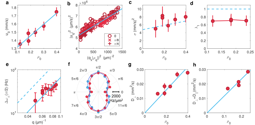
Figure 3: Active-fluid spectroscopy. Red dots: experimental data. Blue line: best linear fit. Dashed line theoretical prediction with no free fitting parameter deduced from kinetic theory, see Supplementary Note 2. The hydrodynamic description of the active fluid is inferred from: a, Variations of the mean-flow speed with the mean area fraction. Error bar: $100\,\rm\mu m/s$, 1std. Denser fluids flow faster. b, Parametric plot of the longitudinal velocity fluctuations $|u_{q}|^{2}$ varrying linearly with $(q_{x}|\rho_{q}|^{2})$ for three propagation angles. The slope gives a measure of $D^{\prime}=4\times 10^{-6}\,\rm mm^{2}/s$. The offset at $q_{x}=0$ comes from the noise acting on the $u$ mode, see Supplementary Note 2. c,d, The compressibility coefficient, $\sigma$ and advection coefficient, $\lambda_{1}$, are plotted versus the mean area fraction $\rho_{0}$. Both quantities are measured from the best fit of the speed of sound (Figs. 2g,  2h,  2). The error bars defined applying the uncertainty-propagation formula on $\sigma=c_{\pm}({\pi/2})^{2}/\rho_{0}$ and $\lambda_{1}=c_{+}(0)/c_{-}(0)$. The uncertainties on $c$ and $\rho_{0}$ are respectively $100\,\rm\mu m/s$ and $0.02$. e, Spectral width $\Delta\omega_{\pm}(\pi/2)$ of the modes propagating at $\theta=\pi/2$ plotted versus $q$ (log-log plot). $\Delta\omega_{\pm}(\pi/2)$ grows quadratically with $q$. Error bars: $10\,\rm Hz$ estimated comparing several Lorentzian fits. Solid line: best quadratic fit. The bare prediction from the simplified kinetic theory overestimates $\Delta\omega_{\pm}(\pi/2)$ by a factor of 3. The possible origins of this overestimate are discussed in Supplementary Note 2. f, Polar plot of the spectral width normalized by $q^{2}$ and averaged over all wave vectors $\Delta_{\pm}=\langle\Delta\omega_{\pm}(\theta)/q^{2}\rangle_{q}$. Red (resp. Blue) dots: experimental data corresponding to $\Delta_{+}$ (resp. $\Delta_{-}$). Solid lines: best fits using the relation $\Delta_{\pm}=\frac{1}{4}[-(D^{\prime}+D_{\perp}+D_{\parallel})-(D^{\prime}+D_{\parallel}-D_{\perp})\cos(2\theta)\pm D_{\rho}u_{0}\sqrt{{\rho_{0}}/{\sigma}}\sin(2\theta)]$, see Supplementary Note 2. g, Variations of the elastic constant $D_{\perp}$ with $\rho_{0}$. $D_{\perp}$ is measured from the quadratic fit shown in e, see main text. Error bars defined as the $0.95$ confidence interval of the quadratic fit in e. The elastic constant increases linearly with the particle density. h, Variations of the average elastic constant $D_{\parallel}+D_{\perp}$ with $\rho_{0}$. $D_{\perp}+D_{\perp}$ measured from the quadratic fit of $\Delta\omega_{+}(\pi/4)+\Delta\omega_{-}(\pi/4)$, see main text. Error bars defined as in g.

Eq. (1) corresponds to mass conservation, and Eq. (Sounds and hydrodynamics of polar active fluids) describes the slow dynamics of the soft transverse-velocity mode. Eq. (3) indicates that $u(\mathbf{r},t)$ is a fast mode. Longitudinal fluctuations quickly relax at all scales and are slaved to $\partial_{x}\rho(\mathbf{r},t)$, see Supplementary Note 2 and Toner and Tu (1995); Marchetti et al. (2013); Mishra et al. (2010). The linear hydrodynamics of the active fluid is therefore fully prescribed by the emergent flow speed $u_{0}(\rho_{{}_{0}})$, Fig. 3a, and six material constants all having a clear physical meaning. $D^{\prime}$ is a diffusion constant readily measured from the linear relation between longitudinal velocity fluctuations and density gradients defined by Eq. (3) and confirmed by Fig 3b. $\lambda_{1}$ measures how fast velocity waves are convected by the mean flow and would be equal to one if momentum were conserved  Toner and Tu (1998). $\sigma$ is the active-liquid compressibility. $D_{\perp}$ and $D_{\parallel}$ can either be thought as viscosities, or orientational elastic constants. Finally $D_{\rm\rho}$ stems for the couplings between orientational and positional degrees of freedom between the active units. Looking for plane-wave solutions of Eqs. (1) and  (Sounds and hydrodynamics of polar active fluids), we readily infer the dispersion relations of mixed density and velocity waves. In the long-wave-length limit, they take the compact form predicted in Toner and Tu (1998): $\omega=\left[c_{\pm}(\theta)q+{\mathcal{O}(q^{2})}\right]+i\Delta\omega_{\pm}(\theta)$, where $c_{\pm}$ is the speed of sound and the imaginary part $\Delta\omega_{\pm}(\theta)={\mathcal{O}}(q^{2})$ corresponds to the widths of the power spectra exemplified in Fig. 2c. The angular variations of the speed of sound are given by:

$$2c_{\pm}(\theta) =\left(1+\lambda_{1}\right)u_{0}\cos\theta$$ (4)

$$\pm\sqrt{\left(\lambda_{1}-1\right)^{2}u_{0}^{2}\cos^{2}\theta+4\sigma\rho_{0}\sin^{2}\theta}.$$

This prediction is in excellent agreement with the speed of sound measurements showed in Figs. 2g, 2h, and 2i for three different densities. As the mean-flow speed $u_{0}(\rho_{0})$ is measured independently, fitting our data requires only two unknown functional parameters $\sigma(\rho_{0})$ and $\lambda_{1}(\rho_{0})$. The variations of $c_{\pm}(\theta)$ therefore provide a direct measurement of the active-fluid compressibility and advection coefficients, Figs. 3c and 3d. The consistency of this method is further established by repeating the same measurements in two different channel geometries, and comparing the density dependence of the hydrodynamic coefficients with the kinetic-theory predictions of  Bricard et al. (2013, 2015); Morin et al. (2016), see Supplementary Note 2. Figure 3c shows a good agreement for the variations of $\sigma(\rho_{0})$ over a range of densities. As in standard liquids, the compressibility increases with $\rho_{0}$. In the case of $\lambda_{1}$ the agreement is also satisfactory but not as accurate, see Fig.3d. Nonetheless theory predicts the correct order of magnitude, and more importantly the absence of variations of $\lambda_{1}$ with $\rho_{0}$. We now measure the elastic constants of the active fluid from the damping of the sound waves. Their damping time is set by the inverse of the spectral widths $\Delta\omega_{\pm}=q^{2}\Delta_{\pm}(\theta)$, where the expression of the angular functions $\Delta_{\pm}(\theta)$ is given in Supplementary Note 2. Fig. 3e agrees with the $q^{2}$ scaling behavior, and we show in Fig. 3f that the angular variations of $\Delta_{\pm}(\theta)$ are correctly fitted by the linear hydrodynamic theory. Given the shape of the power spectra, Fig. 2f, measuring $\Delta_{\pm}$ at small $\theta$ is out of reach of our experiments at high packing fractions. We therefore focus on two high angle values. For $\theta=\pi/2$ and $\theta=\pi/4$, the spectral widths take the simple forms: $\Delta\omega_{\pm}(\pi/2)=q^{2}D_{\perp}/2$ and $\Delta\omega_{\pm}(\pi/4)=q^{2}\left[\frac{1}{4}(D_{\perp}+D_{\parallel}+D^{\prime})\pm(\rho_{0}D_{\rho}u_{0})/\sqrt{4\sigma\rho_{0}}\right]$, as detailed in Supplementary Note 2. A quadratic fit of $\Delta\omega_{\pm}(\pi/2)$ therefore provides a direct measure of $D_{\perp}$, Fig. 3e. Similarly, a quadratic fit of $[\Delta\omega_{+}(\pi/4)+\Delta\omega_{-}(\pi/4)]=\frac{1}{2}(D_{\perp}+D_{\parallel}+D^{\prime})q^{2}$ gives the value of $(D_{\perp}+D_{\parallel})$ as $D^{\prime}=4\times 10^{-6}\,\rm mm^{2}/s$ is four orders of magnitude smaller than $D_{\perp}\sim D_{\parallel}\sim 10^{-2}\,\rm mm^{2}/s$, see Fig 3b. The measured values of the elastic constants $D_{\perp}$ and $D_{\parallel}$ are shown in Figs. 3g and 3h for different packing fractions. Their order of magnitude, Fig. 3e, and more importantly their linear increase with $\rho_{0}$, Figs. 3g and 3h, are consistent with kinetic theory which also predicts that $D^{\prime}$ should be vanishingly small. In principle, $D_{\rho}$ could be measured for any polar active liquid from the value of $\Delta\omega_{+}(\theta)-\Delta\omega_{-}(\theta)\sim D_{\rho}q^{2}$. In the specific case of the colloidal rollers, kinetic theory predicts that $D_{\rho}$ should be independent of $\rho$. The precision of our measurements is however not sufficient for an accurate estimate of the variations of $\Delta\omega_{\pm}$ with the roller fraction. For all fractions below $\rho_{0}=0.24$ we find $D_{\rho}=1\pm 0.5\,10^{-2}\,{\rm mm}^{2}/s$. Analysing the spontaneous fluctuations of the polar active fluids, we have measured all its six materials constants, thereby providing a full description of its linear hydrodynamics.

Before closing this letter, two comments are in order. Firstly, the $q^{2}$ damping of the sound modes implies a $\Delta N^{2}\sim N^{2}$ scaling for the number fluctuations Marchetti et al. (2013). While giant number fluctuations are consistently found in all our experiments, linear theory overestimates their amplitude, see Fig. 1g. This last observation might suggest that the largest scales accessible in our experiments are smaller but not too far from the onset of hydrodynamic breakdown predicted in  Toner and Tu (1995, 1998). Secondly, we here focus on homogeneous active materials. A natural extension to this work concerns sound propagation in more complex active media such as microfluidic lattices Souslov et al. (2017), or curved surfaces Shankar et al. (2017) where topologically-protected chiral sound modes are theoretically predicted.

In conclusion, two decades after the seminal predictions of Toner and Tu, we have experimentally demonstrated that the interplay between motility and soft orientational modes results in sound-wave propagation in colloidal active liquids. We have exploited this counterintuitive phenomenon to lay out a generic spectroscopic method, which could give access to the material constants of all active materials undergoing spontaneous flows. Active-sound spectroscopy applies beyond synthetic active materials Cavagna et al. (2015); Yang and Marchetti (2015), and could be used to quantitatively describe large-scale flocks, schools, and swarms as continuous media Cavagna and Giardina (2014); Ginelli et al. (2015); Buhl et al. (2012); Cavagna et al. (2017).

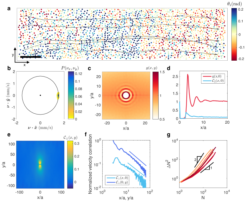
Figure 1: Colloidal rollers self-assemble into a spontaneously-flowing liquid. a, Close up on a microfluidic channel including $\sim 3\times 10^{6}$ colloidal rollers forming a homogeneous polar liquid. The color of the particles indicates the value of the angle, $\theta_{i}$, between their instantaneous velocity and the direction of the mean flow. Five trajectories illustrate the typical motion of the rollers. $\rho_{0}=0.11$. Scale bar: $100\,\rm\mu m$. b, Probability density function of the roller velocities, ${\bf\nu}_{i}(t)$, (ensemble and time integration). All the rollers propel along the same average direction. $\rho_{0}=0.24$ as in all following panels. c, The color indicates the value of the density pair correlation function $g(x,y)$ evaluated at positions $(x,y)$. Structural correlations are short ranged and display only weak anisotropy. d, Cuts along the flow direction of the pair distribution functions, $g(x,0)$ Han (2013), and of the longitudinal velocity correlations ${\mathcal{C}}_{\parallel}(x,0)$, where ${\mathcal{C}}_{\parallel}(\mathbf{r})\equiv\langle\nu_{i}^{\parallel}(t)\nu_{j}^{\parallel}(t)\rangle_{(\mathbf{r}_{i}-\mathbf{r}_{j})=\mathbf{r},t}/\langle(\nu_{i}^{\parallel})^{2}(t)\rangle_{i,t}$. Both structural, and longitudinal- velocity correlations decay over few particle radii. e, Correlations of the transverse velocity fluctuations (ensemble and time average): ${\mathcal{C}}_{\perp}(\mathbf{r})\equiv\langle\nu_{i}^{\perp}(t)\nu_{j}^{\perp}(t)\rangle_{(\mathbf{r}_{i}-\mathbf{r}_{j})=\mathbf{r},t}/\langle(\nu_{i}^{\perp})^{2}(t)\rangle_{i,t}$. The transverse fluctuations are long ranged and strongly anisotropic. f, The correlations of the transverse velocity fluctuations, ${\mathcal{C}}_{\perp}(\mathbf{r})$, decay algebraically in both directions. The solid lines correspond to best algebraic fits: ${\mathcal{C}}_{\perp}(x,0)\sim x^{-0.84}$, and ${\mathcal{C}}_{\perp}(0,y)\sim y^{-0.76}$. g, Giant number fluctuations. Variance, $\Delta N^{2}(\ell)$, of the number of particles measured in square regions of size $\ell$. $\Delta N^{2}(\ell)$ is plotted as a function of the average number of particle $N(\ell)$ for five different polar active liquids of average area fractions $\rho_{0}=0.12,\,0.18,\,0.18,\,0.24,\,0.30,\,0.39$ labeled by colors of increasing darkness. Solid lines: scaling $\Delta N^{2}(\ell)\sim N(\ell)$ corresponding to normal density fluctuations as in equilibrium fluids, and $\Delta N^{2}(\ell)\sim N^{2}(\ell)$ scaling law predicted from linear hydrodynamic theory, see e.g. Marchetti et al. (2013). Details about number fluctuation measurements and power-law fit values are provided in Supplementary Note 1.

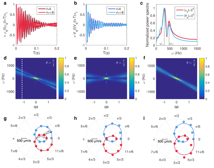
Figure 2: Sound modes in polar active fluids. a, Two-time autocorrelations of the density fluctuations of wave vector $\mathbf{q}$, with $q=0.52\,\mu m^{-1}$, for two different directions of propagations, $\theta=0$ and $\theta=\pi/8$. $\rho_{0}=0.11$. b, Two-time autocorrelations of the transverse velocity fluctuations for the same wave vectors as in $\mathbf{a}$. $\rho_{0}=0.11$. c, Density (red) and velocity (blue) power spectra for $q=0.39$ and $\theta=\pi/4$. The two spectra have two peaks located at the same frequency $\omega_{\pm}$ and have identical width $\Delta\omega_{\pm}$. Both spectra reflect the propagation of the same mixed modes combining velocity and density excitations. $\rho_{0}=0.11$. d, e and f, Full power spectra of the transverse velocity fluctuations $\langle|v_{q,\omega}|^{2}\rangle/\langle|v_{q=0,\omega=0}|^{2}\rangle$. They clearly show the dispersion relations of the mixed sound modes along three different directions $\theta=\pi/4$, $\theta=\pi/2$ and $\theta=\pi/8$. The dashed line in panel d corresponds to the cut showed in c. Sound modes propagate in a non dispersive fashion only at small $q$s. $\rho_{0}=0.11$. g, h and i, Polar plots of the speed of sound, $c_{\pm}(\theta)={\lim_{q\to 0}}[\omega\pm(\theta)/q]$ measured from the slope at $q=0$ of the dispersion relations. Experimental data: Red dots (resp. blue dots) correspond to $c_{+}(\theta)$ (resp. $c_{-}(\theta)$). Solid lines: theoretical fits from Eq. (4). The roller area fractions are $\rho_{0}=0.11$ in g, $\rho_{0}=0.18$ in h, and $\rho_{0}=0.24$ in i.

Acknowledgements. We acknowledge support from ANR program MiTra and Institut Universitaire de France. We thank O. Dauchot, A. Souslov and especially H. Chaté, B. Mahault, S. Ramaswamy, Y. Tu and J. Toner for invaluable comments and discussions.
Author Contributions. D. B. conceived the project. D. G. and D. B. designed the experiments. D. G. and A. M. performed the experiments. D. G. and D. B. analyzed and discussed the results. D. G. and D. B. wrote the paper.
Author Information. Correspondence and requests for materials should be addressed to D. B. (email: denis.bartolo@ens-lyon.fr).

Methods

We use Polystyrene colloids of diameter $2a=4.8\,\rm\mu m$ dispersed in a 0.15 mol.L^-1 AOT-hexadecane solution (Thermo scientific G0500). The suspension is injected in a wide microfluidic channel made of two parallel glass slides coated by a conducting layer of Indium Tin Oxyde (ITO) (Solems, ITOSOL30, thickness: 80 nm) Bricard et al. (2013). The two electrodes are assembled with double-sided scotch tape of homogeneous thickness ($H=110\,\mu\rm m$). More details about the design of the microfluidic device are provided in the Supplementary Figure 5.

The colloids are confined in a $2\,\rm mm\times 30\,mm$ race track. The walls are made of a positive photoresist resin (Microposit S1818, thickness: 2 $\mu$m). This geometry is achieved by means of conventional UV lithography. After injection the colloids are let to sediment onto the positive electrode. Once a monolayer forms, Quincke electro-rotation is achieved by applying a homogeneous electric field transverse to the two electrodes $\mathbf{E}=E_{0}\hat{\mathbf{z}}$. The field is applied with a voltage amplifier (TREK 609E-6). All reported results correspond to an electric field $E_{0}=2E_{\rm Q}$, where $E_{\rm Q}$ is the Quincke electro-rotation threshold $E_{\rm Q}=1\,\rm V/\mu m$. The colloids are electrostatically repelled from the regions covered by the resin film thereby confining the active liquid in the racetrack. Upon applying $E_{0}$ the rollers propel instantly and quickly self-organize into a spontaneously flowing colloidal liquid. All measurements are performed after the initial density heterogeneities have relaxed and a steady state is reached for all the observables. The waiting time is typically of the order of 10 minutes.

The colloids are observed with a 9.6x magnification with a fluorescent Nikon AZ100 microscope. The movies are recorded with a $4\,\rm Mpix$ CMOS camera (Basler ACE) at frame rates of 500 fps. The particles are detected with a one pixel accuracy, and the particle trajectories and velocities are reconstructed using the Crocker and Grier algorithm [35]. Measurements are performed in a $1146\,\rm\mu m\times 286\,\rm\mu m$ observation window. The individual particle velocities are averaged over 4 subsequent frames.

The spatial Fourier transform of the density and transverse velocity fields are respectively defined as:

$$\rho_{q}(t) =\sum_{i}e^{iq\left[x_{i}(t)\cos\theta+y_{i}(t)\sin\theta\right]},$$ (5)

$$\mathbf{v}_{q}(t) =\sum_{i}{\bm{\nu}}_{i}(t)e^{iq\left[x_{i}(t)\cos\theta+y_{i}(t)\sin\theta\right]},$$ (6)

where $x_{i}(t)$ and $y_{i}(t)$ are the instantaneous particle coordinates. The sum is performed over all detected particles. Time Fourier transforms are then performed using the MATLAB implementation of the FFT algorithm. The positions of the maxima, $\omega_{\pm}$, and the width $\Delta\omega_{\pm}$ of the velocity power spectra are determined by fitting the $|v_{q}(\omega)|^{2}$ curve by the sum of two Lorentzian functions.

Code avaibility

Matlab scripts used in this work are avaible from the corresponding author upon reasonnable request.

Data avaibility

The data that support the findings of this study are avaible upon request from the corresponding author.

Methods Reference

[35] John Cocker and David Grier, ”Methods of digital video microscopy for colloidal studies”, Journal of colloid and interface science (1996).

References

- Schaller et al. (2010) Volker Schaller, Christoph Weber, Christine Semmrich, Erwin Frey, and Andreas R Bausch, “Polar patterns of driven filaments,” Nature 467, 73 (2010).
- Sanchez et al. (2012) Tim Sanchez, Daniel T. N. Chen, Stephen J. DeCamp, Michael Heymann, and Zvonimir Dogic, “Spontaneous motion in hierarchically assembled active matter,” Nature 491, 431–434 (2012).
- Wioland et al. (2013) Hugo Wioland, Francis G. Woodhouse, Jörn Dunkel, John O. Kessler, and Raymond E. Goldstein, “Confinement stabilizes a bacterial suspension into a spiral vortex,” Phys. Rev. Lett. 110, 268102 (2013).
- DeCamp et al. (2015) Stephen J. DeCamp, Gabriel S. Redner, Aparna Baskaran, Michael F. Hagan, and Zvonimir Dogic, “Orientational order of motile defects in active nematics,” Nature Materials 14, 1110–1115 (2015).
- Nishiguchi et al. (2017) Daiki Nishiguchi, Ken H. Nagai, Hugues Chaté, and Masaki Sano, “Long-range nematic order and anomalous fluctuations in suspensions of swimming filamentous bacteria,” Phys. Rev. E 95, 020601 (2017).
- Ellis et al. (2017) Perry W. Ellis, Daniel J. G. Pearce, Ya-Wen Chang, Guillermo Goldsztein, Luca Giomi, and Alberto Fernandez-Nieves, “Curvature-induced defect unbinding and dynamics in active nematic toroids,” Nature Physics (2017).
- Deseigne et al. (2010) Julien Deseigne, Olivier Dauchot, and Hugues Chaté, “Collective motion of vibrated polar disks,” Phys. Rev. Lett. 105, 098001 (2010).
- Bricard et al. (2013) Antoine Bricard, Jean-Baptiste Caussin, Nicolas Desreumaux, Olivier Dauchot, and Denis Bartolo, “Emergence of macroscopic directed motion in populations of motile colloids,” Nature 503 (2013).
- Chen et al. (2011) Qian Chen, Sung Chul Bae, and Steve Granick, “Directed self-assembly of a colloidal kagome lattice,” Nature 469, 381 (2011).
- Kumar et al. (2014) Nitin Kumar, Harsh Soni, Sriram Ramaswamy, and AK Sood, “Flocking at a distance in active granular matter,” Nature Communications 5 (2014).
- Nishiguchi and Sano (2015) Daiki Nishiguchi and Masaki Sano, “Mesoscopic turbulence and local order in janus particles self-propelling under an ac electric field,” Phys. Rev. E 92, 052309 (2015).
- Toner and Tu (1995) John Toner and Yuhai Tu, “Long-range order in a two-dimensional dynamical model: How birds fly together,” Phys. Rev. Lett. 75, 4326–4329 (1995).
- Toner and Tu (1998) John Toner and Yuhai Tu, “Flocks, herds, and schools: A quantitative theory of flocking,” Phys. Rev. E 58, 4828–4858 (1998).
- Tu et al. (1998) Yuhai Tu, John Toner, and Markus Ulm, “Sound waves and the absence of galilean invariance in flocks,” Phys. Rev. Lett. 80, 4819–4822 (1998).
- Aditi Simha and Ramaswamy (2002) R. Aditi Simha and Sriram Ramaswamy, “Hydrodynamic fluctuations and instabilities in ordered suspensions of self-propelled particles,” Phys. Rev. Lett. 89, 058101 (2002).
- Shankar et al. (2017) Suraj Shankar, Mark J. Bowick, and M. Cristina Marchetti, “Topological sound and flocking on curved surfaces,” Phys. Rev. X 7, 031039 (2017).
- Souslov et al. (2017) Anton Souslov, Benjamin C Van Zuiden, Denis Bartolo, and Vincenzo Vitelli, “Topological sound in active-liquid metamaterials,” Nature Physics (2017).
- Cavagna and Giardina (2014) Andrea Cavagna and Irene Giardina, “Bird flocks as condensed matter,” Annual Review of Condensed Matter Physics 5, 183–207 (2014).
- Ginelli et al. (2015) Francesco Ginelli, Fernando Peruani, Marie-Hel ne Pillot, Hugues Chaté, Guy Theraulaz, and Richard Bon, “Intermittent collective dynamics emerge from conflicting imperatives in sheep herds,” Proceedings of the National Academy of Sciences 112, 12729–12734 (2015).
- Buhl et al. (2012) J Buhl, Gregory A Sword, and Stephen J Simpson, “Using field data to test locust migratory band collective movement models,” Interface Focus 2, 757–763 (2012).
- Cavagna et al. (2017) Andrea Cavagna, Daniele Conti, Chiara Creato, Lorenzo Del Castello, Irene Giardina, Tomas S Grigera, Stefania Melillo, Leonardo Parisi, and Massimiliano Viale, “Dynamic scaling in natural swarms,” Nature Physics 13 (2017).
- Quincke (1896) G. Quincke, “Uber rotationen im constanten electrischen felde,” Annalen der Physik , 417–486 (1896).
- Melcher and Taylor (1969) J. R. Melcher and G. I. Taylor, “Electrohydrodynamics: A review of the role of interfacial shear stresses,” Annual Review of Fluid Mechanics 1, 111–146 (1969).
- Lavrentovich (2016) Oleg D. Lavrentovich, “Active colloids in liquid crystals,” Current Opinion in Colloid & Interface Science 21 (2016).
- Toner et al. (2005) John Toner, Yuhai Tu, and Sriram Ramaswamy, “Hydrodynamics and phases of flocks,” Annals of Physics 318, 170 – 244 (2005), special Issue.
- Marchetti et al. (2013) M. C. Marchetti, J. F. Joanny, S. Ramaswamy, T. B. Liverpool, J. Prost, Madan Rao, and R. Aditi Simha, “Hydrodynamics of soft active matter,” Rev. Mod. Phys. 85, 1143–1189 (2013).
- Daniels and Durian (2011) L. J. Daniels and D. J. Durian, “Propagating waves in a monolayer of gas-fluidized rods,” Phys. Rev. E 83, 061304 (2011).
- Kyriakopoulos et al. (2016) Nikos Kyriakopoulos, Francesco Ginelli, and John Toner, “Leading birds by their beaks: the response of flocks to external perturbations,” New Journal of Physics 18, 073039 (2016).
- Mishra et al. (2010) Shradha Mishra, Aparna Baskaran, and M. Cristina Marchetti, “Fluctuations and pattern formation in self-propelled particles,” Phys. Rev. E 81, 061916 (2010).
- Bricard et al. (2015) Antoine Bricard, Jean-Baptiste Caussin, Debasish Das, Charles Savoie, Vijayakumar Chikkadi, Kyohei Shitara, Oleksandr Chepizhko, Fernando Peruani, David Saintillan, and Denis Bartolo, “Emergent vortices in populations of colloidal rollers,” Nature communications 6 (2015).
- Morin et al. (2016) Alexandre Morin, Nicolas Desreumaux, Jean-Baptiste Caussin, and Denis Bartolo, “Distortion and destruction of colloidal flocks in disordered environments,” Nature Physics 1, 1–6 (2016).
- Cavagna et al. (2015) Andrea Cavagna, Irene Giardina, Tomas S. Grigera, Asja Jelic, Dov Levine, Sriram Ramaswamy, and Massimiliano Viale, “Silent flocks: Constraints on signal propagation across biological groups,” Phys. Rev. Lett. 114, 218101 (2015).
- Yang and Marchetti (2015) Xingbo Yang and M. Cristina Marchetti, “Hydrodynamics of turning flocks,” Phys. Rev. Lett. 115, 258101 (2015).
- Han (2013) “Theory of simple liquids,” in Theory of Simple Liquids (Fourth Edition), edited by Jean-Pierre Hansen and Ian R. McDonald (Academic Press, Oxford, 2013) fourth edition ed.