Optimal Adaptive and Accelerated Stochastic Gradient Descent

Abstract

Stochastic gradient descent (Sgd) methods are the most powerful optimization tools in training machine learning and deep learning models. Moreover, acceleration (a.k.a. momentum) methods and diagonal scaling (a.k.a. adaptive gradient) methods are the two main techniques to improve the slow convergence of Sgd. While empirical studies have demonstrated potential advantages of combining these two techniques, it remains unknown whether these methods can achieve the optimal rate of convergence for stochastic optimization. In this paper, we present a new class of adaptive and accelerated stochastic gradient descent methods and show that they exhibit the optimal sampling and iteration complexity for stochastic optimization. More specifically, we show that diagonal scaling, initially designed to improve vanilla stochastic gradient, can be incorporated into accelerated stochastic gradient descent to achieve the optimal rate of convergence for smooth stochastic optimization. We also show that momentum, apart from being known to speed up the convergence rate of deterministic optimization, also provides us new ways of designing non-uniform and aggressive moving average schemes in stochastic optimization. Finally, we present some heuristics that help to implement adaptive accelerated stochastic gradient descent methods and to further improve their practical performance for machine learning and deep learning.

1 Introduction

In this paper we are interested in solving the following optimization problem:

$$\min_{x} \quad f(x):=\mathbb{E}[F(x,\xi)]$$

s.t. $$\quad x\in\mathcal{X}$$ (1)

where $\mathcal{X}$ is a closed convex set in $\mathbb{R}^{d}$, $F(\cdot,\xi):\mathcal{X}\to\mathbb{R}$ is a continuously differentiable function and $\xi\in\Xi\subset\mathbb{R}^{p}$ is a random variable.

The stochastic gradient descent method is obtained from gradient descent by replacing the exact gradient $g(x)=\nabla f(x)$ with a stochastic gradient $G(x,\xi)=\partial_{x}F(x,\xi)$, where $\xi$ is random samples. Sgd was initially presented in a seminal work by Robbins and Monro [23] and later significantly improved in [15, 20, 21, 14] through the incorporation of averaging and adaption to problem geometry. Sgd methods are now the de-facto techniques to tackle the optimization problems for training large-scale machine learning and deep learning models.

While momentum methods, first pioneered by Polyak ([19]) and later significantly improved in Nesterov’s work [17, 16], are well-known techniques to accelerate deterministic smooth convex optimization, only recently have these techniques been incorporated into stochastic optimization starting from [12, 11]. Under convex assumptions, Nesterov’s method and its stochastic counterparts have been shown to exhibit the optimal convergence rates for solving different classes of problems. These methods have also been recently generalized for solving nonconvex and stochastic optimization problems [6]. [25] demonstrated the importance of momentum and advantage of Nesterov’s accelerated gradient method in training deep neural nets. Recent works [7, 9] propose more robust accelerated Sgd with improved statistical error. In addition, many studies investigate convergence issue for nonconvex optimization, including the theoretical concern on the convergence to saddle point and how to escape from that. [13, 5] show that gradient descent in general converges to local optima. By utilizing second-order information, one can obtain improved rate of convergence to approximate local minima. This includes approaches based on Nesterov and Polyak’s cubic regularization [1, 18, 27], or first-order method with accelerated gradient method as a sub-solver for escaping saddle points [2].

In a different line of research, adaptive stepsizes to each decision variable have been used to incorporate information about geometry of data more efficiently. Built upon mirror-descent [14, 15] and diagonal scaling, the earlier work [4] proposes AdaGrad, an adaptive subgradient method that has been widely applied to online and stochastic optimization. Later [30, 22, 3, 10, 26] exploit adaptive Sgd, referred to as Adam, for optimizing deep neural networks. Their studies suggest that exponential moving average, which leans towards the later iterates, often outperform AdaGrad, which weighs the iterates equally. The work [3] empirically combines accelerated gradient with Adam. However, there is no theoretical analysis and the interplay between momentum and adaptive stepsize remains unclear. In addition, the theoretical insight of exponential moving average is not well understood. In particular, recent work [22] addresses the non-convergent issue of Adam, a popular exponential averaging Sgd, and proposes a modified averaging scheme with guaranteed convergence. The work [29] questions the generalization ability of adaptive methods compared to Sgd. Later [8] develops a strategy to switch from Adam to Sgd for enhancing generalization performance while retaining the fast convergence on the initial phase.

Our goal in this paper is to develop a new accelerated stochastic gradient descent, namely A2Grad, by showing in theory how adaptive stepsizes should be chosen in the framework of accelerated methods. Our main contribution are as follows:

1. A clean complexity view of adaptive momentum methods. We show that adaptive stepsizes can improve the convergence of stochastic component while Nesterov’s accelerated method improves the deterministic and smooth part. In particular, A2Grad not only achieves the optimal $\mathcal{O}(\frac{L}{k^{2}}+\frac{\sigma}{\sqrt{k}})$ worst-case rate of convergence for stochastic optimization as shown in [12], but can also improve significantly the second term by adapting to data geometry. Here $L$ denotes the Lipschitz constant for the gradient $\nabla f$, $\sigma$ denotes the variance of stochastic gradient and $k$ denotes the iteration number.

2. Our paper provides a more general framework to analyze adaptive accelerated methods—not only including AdaGrad-type moving average, but also providing new ones—with unified theory. We show that momentum also guide us to design incremental and adaptive stepsizes that beyond the choices in existing work. One can choose between uniform average and nonuniform average up to quadratic weights in the adaptive stepsize while retaining the optimal rate.

3. Our theory also includes exponential moving average as a special case and for the first time, has obtained the nearly-optimal convergence under sub-Gaussian assumption. The rate can be further improved to optimal under assumption of bounded gradient norm.

The rest of the paper proceeds as follows. Section 2 introduces the accelerated Sgd and adaptive Sgd. Section 3 states our main contribution which presents a new A2Grad framework of developing accelerated Sgd. Section 4 discusses several adaptive gradient strategies. Section 5 conducts experiments to the empirical advantage of our approach. Finally we draw several conclusions in Section 6.

Notation.

For a vector $x\in\mathbb{R}^{d}$, we use $x^{2}$ to denote element-wise square and $\sqrt{x}$ to denote the element-wise square root. For vectors $x$ and $y$, $xy$ and $\frac{x}{y}$ denote the element-wise multiplication and division respectively. With slight abuse of notation, $x_{i}$ denotes the $i$-th coordinate of vector $x$, and $x_{k,i}$ denotes the $i$-th coordinate of vector $x_{k}$. For a sequence of vectors $x_{k},x_{k+1},...,x_{t}$ where $k\leq t$, we use $x_{k:t,i}$ to denote the vector $[x_{k,i},x_{k+1,i},...,x_{t,i}]^{T}$ .

2 Stochastic gradient descent

The last few years has witnessed the great success of Sgd type methods in the field of optimization and machine learning. For many learning tasks, Sgd converges slowly and momentum method improves Sgd by adding inertia of the iterates to accelerate the optimization convergence. However, classical momentum method does not guarantee optimal convergence, except for some special cases. Under the convex assumption, Nesterov developed the celebrated accelerated gradient (NAG) method which achieves the optimal rate of convergence. By presenting a unified analysis for smooth and stochastic optimization, and carefully designing the stepsize policy, [12] studies a variant of Nesterov’s accelerated gradient method that exhibits the optimal convergence for convex stochastic optimization. The optimal accelerated stochastic approximation method in [12] converges at the rate of $\mathcal{O}(\frac{L}{k^{2}}+\frac{\sigma}{\sqrt{k}})$, much better than vanilla Sgd with a rate of $\mathcal{O}(\frac{L}{k}+\frac{\sigma}{\sqrt{k}})$ for solving ill-conditioned problems with large constant $L$. Later work [25] investigates the performance of Sgd on training deep neural networks, and demonstrates the importance of momentum, in particular, the advantage of Nesterov’s acceleration in training deep neural networks.

Input: $x_{0}$, $v_{0}$

for k=0,1,2,…,K do

       Obtain sample $\xi_{k}$ and compute $G_{k}\in\nabla F(x_{k},\xi_{k})$;

       $v_{k}=\psi(G^{2}_{0},G^{2}_{1},G^{2}_{2},...,G^{2}_{k})$;

       $\tilde{G}_{k}=\phi(G_{0},G_{1},G_{2},...,G_{k})$;

       $x_{k+1}=x_{k}-\beta_{k}\tilde{G}_{k}/\sqrt{v_{k}}$;

      

end for

Output: $x_{K+1}$

Algorithm 1 Adaptive method

However, since both Sgd and momentum methods only depend on a single set of parameters for tuning all the coordinates, they can be inefficient for ill-posed and high dimensional problems. To overcome these shortcomings, adaptive methods perform diagonal scaling on the gradient by incorporating the second moment information. We describe a general framework of adaptive gradient in Algorithm 1, where $\psi$ and $\phi$ are some weighing functions. For example, the original AdaGrad ([4]) takes adaptive stepsize in the following form:

$$v_{k} =v_{k-1}+G_{k}^{2}$$

$$x_{k+1} =x_{k}-\frac{\beta_{k}}{\sqrt{v_{k}}}G_{k}.$$

In deep learning, the optimization landscape can be very different from that of convex learning models. It seems to be intuitive to put higher weights on the later iterates in the optimization trajectory. Consequently, adaptive methods including Rmsprop[26], Adadelta [30], Adam [10] and several others propose more practical adaptive methods with slightly different schemes to exponentially average the past second moment.

Both momentum and adaptive gradient improve the performance of Sgd and quickly become popular in machine learning. However, these two techniques seem to improve Sgd on some orthogonal directions. Momentum aims at changing the global dynamics of learning system while adaptive gradient aims at making Sgd more adaptive to the local geometry. The convergence of adaptive gradient is first established for AdaGrad and later extended to adaptive momentum methods with exponential moving average. However the proof of all these work seems to be based on regret analysis and subgradient methods. When applying momentum based adaptive gradients for smooth optimization, the theory only guarantees a convergence rate of $O(\frac{1}{\sqrt{k}})$, much worse than the $O(\frac{1}{k^{2}})$ achieved by other accelerated methods. Thus it is natural to ask the question: Can momentum truly help improve the convergence of adaptive gradient methods?

3 Adaptive ASGD

To answer this question, we will base our study on accelerated gradient method using Nesterov’s momentum. Our main goal in this section is to develop a novel accelerated stochastic gradient method by combining the advantage of Nesterov’s accelerated gradient method and adaptive gradient method with stepsize tuned per parameter. We will discuss the interplay of these two strategies and develop new moving average schemes to further accelerate convergence.

We begin with several notations. Define $D_{\phi}(y,x)=\phi(x)-\phi(y)-\left\langle\nabla\phi(y),x-y\right\rangle$ as a Bregman divergence where the convex smooth function $\phi(\cdot)$ is called a proximal function or distance generating function in the literature of mirror descent. We assume that $\phi(x)$ is 1-strongly convex with respect to the semi-norm $\|\cdot\|_{\phi}$, or equivalently, $D_{\phi}(x,y)\geq\frac{1}{2}\|x-y\|_{\phi}^{2}$. Also let $\|\cdot\|_{\phi*}$ be the dual norm associated with $\|\cdot\|_{\phi}$. Many popular optimization algorithms, such as gradient descent, adopt $D_{\phi}(x,y)=\frac{1}{2}\|x-y\|^{2}$, simply by setting proximal function according to the Euclidean norm: $\phi(x)=\frac{1}{2}\|x\|^{2}$. In contrast, adaptive gradient methods apply data-driven $\phi_{k}(x)$ $(k\geq 0)$ which is adaptive to the past (sub)gradient.

In Algorithm 2, we propose a general algorithmic framework: adaptive accelerated stochastic gradient (A2Grad) method, of which the main idea is to apply extra adaptive proximal function in the process of accelerated gradient methods while retaining the optimal convergence imposed by Nesterov’s momentum. Examining step (3) in the algorithm, the major difference between A2Grad and the other stochastic accelerated gradient descent exists in that the new update couples the two Bregman distance $D(x_{k},x)$ and $D_{\phi_{k}}(x_{k},x)$, controlled by stepsize $\gamma_{k}$ and $\beta_{k}$ respectively. The first one $D(y,x)$ is short for $D_{\psi}(y,x)$, where $\psi$ can be any fixed convex proximal function during the optimization iterations. For practical purpose, in this paper we will use $\psi(x)=\frac{1}{2}\|x\|^{2}$ and then skip the subscript for the sake of simplicity. On the other hand, $D_{\phi_{k}}(x_{k},x)$ uses a variable proximal function, allowing gradual adjustment when algorithm proceeds. As a consequence, the mirror descent update is a joint work of both Nesterov’s momentum and adaptive gradient. Although the view of two Bregman divergence seems straightforward, it provide us with a clearer vision on the interaction between Nesterov’s term and adaptive gradient. As we shall see later, our framework leads to novel adaptive moving average with sharper theoretical guarantee.

In the following theorem, we provide the first main result on the general convergence property of A2Grad. The proof of the theorem is left in Appendix for brevity.

Input: $x_{0}$, $\bar{x}_{0}$, $\gamma_{k},\beta_{k}>0$

for $k=0,1,2\ldots K$ do

       Update:

$$\underline{x}_{k}=(1-\alpha_{k})\bar{x}_{k}+\alpha_{k}x_{k}$$ (2)

Sample $\xi_{k}$, compute $\underline{G}_{k}\in\nabla F(\underline{x}_{k},\xi_{k})$ and $\phi_{k}(\cdot)$, then update:

      

$$x_{k+1} =\operatornamewithlimits{argmin}_{x\in\mathcal{X}}\left\{\left\langle\underline{G}_{k},x\right\rangle+\gamma_{k}D(x_{k},x)+\beta_{k}D_{\phi_{k}}(x_{k},x)\right\}$$ (3)

$$\bar{x}_{k+1} =(1-\alpha_{k})\bar{x}_{k}+\alpha_{k}x_{k+1}$$ (4)

end for

Output: $\bar{x}_{K+1}$

Algorithm 2 Adaptive accelerated stochastic gradient (A2Grad) algorithm

Theorem 1.

In Algorithm 2, if $f$ is convex and Lipschitz smooth with constant $L$, and $\{\alpha_{k}\}$ and $\{\gamma_{k}\}$ satisfy the following conditions:

$$L\alpha_{k} \leq\gamma_{k},$$ (5)

$$\lambda_{k+1}\alpha_{k+1}\gamma_{k+1} \leq\lambda_{k}\alpha_{k}\gamma_{k},$$ (6)

where the sequence $\{\lambda_{k}\}$ is defined by $\lambda_{k}=1/\prod_{i=1}^{k}(1-\alpha_{i}),k=1,2,3...,\;\text{and\ }\lambda_{0}=1,$ then

$$\lambda_{K}\left[f(\bar{x}_{K+1})-f(x)\right]\leq(1-\alpha_{0})\left[f(\bar{x}_{0})-f(x)\right]+\alpha_{0}\gamma_{0}D(x_{0},x)+\sum_{k=0}^{K}\lambda_{k}[\frac{\alpha_{k}\|\delta_{k}\|_{\phi_{k}*}^{2}}{2\beta_{k}}+\alpha_{k}\left\langle\delta_{k},x-x_{k}\right\rangle+\alpha_{k}R_{k}],$$ (7)

where $\delta_{k}=\underline{G}_{k}-\nabla f(x_{k})$ and $R_{k}=\beta_{k}D_{\phi_{k}}(x_{k},x)-\beta_{k}D_{\phi_{k}}(x_{k+1},x).$

Let us make a few comments about Theorem 1. First, the parameters $\{\gamma_{k}\}$ and $\{\alpha_{k}\}$ satisfy some recursion that are typical for Nesterov’s accelerated method [28]; their choices are crucial to guarantee optimal convergence in convex smooth optimization. Second, the dynamics of adaptive gradient exhibits a new pattern, crucially differing from many other adaptive methods such as AdaGrad, Adam and Nadam. Thanks to the momentum, the pattern renders a novel interplay of proximal function $\phi_{k}$ with variance of stochastic gradient: $\|\delta_{k}\|_{\phi_{k}^{*}}$, instead of with (sub)gradient norm $\|\underline{G}_{k}\|_{\phi_{k}^{*}}$. Finally, we need to mention that the discussion so far is still conceptual, since the parameters have not been fixed yet. In particular, one important remaining issue is to select appropriate proximal function $\phi_{k}$. Hereafter, the paper will be devoted to deriving more specific choices of these parameters.

4 Diagonal scaling and moving average schemes

There are many different ways to choose the underlying proximal function $\phi_{k}$. For practical use, we adopt diagonal scaling function :$\phi_{k}(x)=\frac{1}{2}\|x\|^{2}_{h_{k}}=\frac{1}{2}\langle x^{T},\text{Diag}(h_{k})x\rangle$, where $h_{k}\in\mathbb{R}^{d}$ and $h_{k,i}>0$, $1\leq i\leq d$. Consequently, the Bregman divergence has the following form: $D_{\phi_{k}}(x,y)=\frac{1}{2}\langle(x-y)^{T}\text{Diag}(h_{k})(x-y)\rangle$ and $\ D(x,y)=\frac{1}{2}\|x-y\|^{2}.$

Compute $h_{k}$ and replace the update of $x_{k+1}$ in (3) by

$$x_{k+1}=\Pi_{\mathcal{X}}(x_{k}-\frac{1}{\gamma_{k}+\beta_{k}h_{k}}\underline{G}_{k}),$$

where $\Pi_{\mathcal{X}}$ denotes the projection operator over $\mathcal{X}$.

Algorithm 3 A2Grad with diagonal scaling

In addition, a crucial step to guarantee convergence is to ensure that the sum $\sum_{k}\lambda_{k}\alpha_{k}R_{k}$ does not grow too fast. One sufficient condition is to ensure that for any $k\geq 0$:

$$\lambda_{k}\alpha_{k}\beta_{k}D_{\phi_{k}}(x_{k},x)\geq\lambda_{k-1}\alpha_{k-1}\beta_{k-1}D_{\phi_{k}}(x_{k-1},x).$$ (8)

We describe a specific variant of A2Grad using diagonal scaling function in Algorithm 3, and provide a general scheme to choose its parameters. The convergence of Algorithm 3 is summarized in the following theorem.

Theorem 2.

Let $x^{*}$ be an optimal solution. Also assume $\|x_{k}-x^{*}\|_{\infty}^{2}\leq B$ for some $B>0$ (this assumption is satisfied, e.g., when $\mathcal{X}$ is compact). In Algorithm 3, if $\alpha_{k}=\frac{2}{k+2}$, $\gamma_{k}=\frac{2L}{k+1}$ and $\{\beta_{k},h_{k}\}$ satisfy the monotone property

$$\lambda_{k+1}\alpha_{k+1}\beta_{k+1}h_{k+1,i}\geq\lambda_{k}\alpha_{k}\beta_{k}h_{k,i},$$

$$\forall k=0,1,2,...,1\leq i\leq d,$$

then we have

$$\mathbb{E}\left[f(\bar{x}_{K+1})-f(x^{*})\right]\leq\frac{2L\|x^{*}-x_{0}\|^{2}}{(K+1)(K+2)}+\frac{2B\beta_{K}\mathbb{E}\left[\sum_{i=1}^{d}h_{K}^{(i)}\right]}{K+2}+\sum_{k=0}^{K}\mathbb{E}\left\{\frac{(k+1)\|\delta_{k}\|_{h_{k}*}^{2}}{\beta_{k}(K+1)(K+2)}\right\}.$$

The main message of Theorem 2 is that the complexity rate of A2Grad can be viewed as the sum of deterministic dynamics and stochastic dynamics. The proximal function $h_{k}$ exhibits an interplay with variance $\delta_{k}$ instead of $\|\underline{G}_{k}\|^{2}$, which is commonly seen in existing adaptive methods. Notably, such interplay between $h_{k}$ and $\delta_{k}$ is essential to make efficient use of momentum, because now momentum term can significantly accelerate convergence of deterministic dynamics while adaptive gradient will concentrate on the stochastic dynamics. Moreover, thanks to the momentum, the bound on stochastic part is more complicated than that of adaptive gradient. As we will see soon, it provides us a rich source of adaptive stepsizes.

Uniform vs nonuniform moving average

Our goal is to design specific adaptive stepsizes with guaranteed theoretical convergence. For the moment let us assume that the full gradient $g_{t}$ is known. The adaptive function $h_{k}$ will be chosen as a square root of the weighted sum of sequence $\{\delta_{k}^{2}\}$. Immediately we conclude the convergence rate in the following corollary.

Corollary 1.

Under the assumption of Theorem 2, let $\beta_{k}=\beta$ and

$$h_{k}=\frac{1}{(k+1)^{q/2}}\sqrt{\sum_{\tau=0}^{k}(\tau+1)^{q}\delta_{\tau}^{2}}\ \text{ with }\ q\in[0,2],$$

then we have

$$\mathbb{E}\left[f(\bar{x}_{K+1})-f(x^{*})\right]\leq\frac{2L\|x-x_{0}\|^{2}}{(K+1)(K+2)}+\frac{2\mathbb{E}\left[\sum_{i=1}^{d}\|\delta_{0:K,i}\|\right]}{\beta(K+2)}+\frac{2\beta B\ \mathbb{E}\left[\sum_{i=1}^{d}\|\delta_{0:K,i}\|\right]}{K+2}.$$

In Corollary 1, the stochastic part is related to the expected sum of $\|\delta_{0:K,i}\|$, for $i=1,2,...,d$. Under the mild assumption of bounded variance, namely, for $x\in\mathcal{X}$, $\mathbb{E}_{\xi}\|G(x,\xi)-g(x,\xi)\|^{2}\leq\sigma^{2}$, where $\sigma>0$, we have

$$\mathbb{E}[\|\delta_{0:K,i}\|]\leq\sqrt{\sum_{k=0}^{K}\mathbb{E}[\delta_{k,i}^{2}]}\leq\sqrt{K+1}\sigma$$

by Jensen’s inequality. Hence the stochastic part obtains the $\mathcal{O}(\frac{1}{\sqrt{K}})$ rate of convergence. Moreover, the convergence rate also suggests that there exists an optimal $\beta$ to minimize the bound. However, such optimal value is rarely known and will be a hyper-parameter for tuning in the practice.

Furthermore, Corollary 1 allows us to choose a family of adaptive functions. Next we will consider two specific choices. By setting $q=0$, we arrive at uniform moving average for forming the diagonal function: $h_{k}=\sqrt{\sum_{\tau=0}^{k}\delta_{\tau}^{2}}.$ We describe A2Grad with this choice in Algorithm 4.

Input: $v_{-1}=0$ and the rest of other parameters

The $k$-th step of Algorithm 3:

$$v_{k} =v_{k-1}+\delta_{k}^{2}$$

$$h_{k} =\sqrt{v_{k}}$$

Algorithm 4 A2Grad-uni: Adaptive ASGD with uniform moving average

Setting $q=2$, we arrive at an incremental moving average with quadratic weight: $h_{k}$ by $h_{k}=\frac{1}{(k+1)}\sqrt{\sum_{\tau=0}^{k}(\tau+1)^{2}\delta_{\tau}^{2}}.$ We describe A2Grad with such incremental scheme in Algorithm 5. Compared with uniform averaging, the scaling vectors $\delta_{k}$ will first shrink by a factor $\frac{k^{2}}{(k+1)^{2}}$ before adding the new iterate. On the long run, the earlier scales will have a relative weights decaying at the rate of $\mathcal{O}(\frac{1}{k^{2}}$). To our best knowledge, this is the first study on using nonlinear polynomial weights in the work of adaptive gradient methods, and the first study of using nonlinear weights without introducing an additional $\mathcal{O}(\log{k})$ factor in the complexity bound.

Input: $v_{-1}=0$ and the rest of other parameters

The $k$-th step of Algorithm 3:

$$v_{k} =k^{2}/(k+1)^{2}v_{k-1}+\delta_{k}^{2}$$

$$h_{k} =\sqrt{v_{k}}$$

Algorithm 5 A2Grad-inc: Adaptive ASGD with incremental moving average (quadratic weight)

Exponential moving average

Besides the uniform and nonuniform schemes discussed above, it is important to know whether exponential moving average—a popular choice in deep learning area—can be combined with Nesterov’s accelerated method with justified theoretical convergence.

A crucial difference between the family of adaptive gradients by exponential moving averages and the earlier AdaGrad in how the diagonal terms are accumulated. Typically, exponential average methods apply the update

$$v_{k}=\theta v_{k-1}+(1-\theta)G_{k}^{2},\quad h_{k}=\sqrt{v_{k}}$$ (9)

with $\theta\in(0,1)$ for deriving the diagonal term. Although exp-avg methods have received popularity in deep learning field, their theoretical understanding is limited and their convergence performance remains a question. In particular, recent [22] provides a simple convex problem on which Adam fails to converge easily. The intuition of such phenomenon is as follows. Generally, to ensure algorithm convergence, SGD reduces the influence of variance of stochastic gradients by applying diminishing stepsize $\eta_{k}:\eta_{k}\rightarrow 0$ as $k\rightarrow 0$. In Adam and many other exp-avg methods, the effective stepsize $\eta_{k}$ is controlled by the scaling term $h_{k}$ with $\eta_{k}\propto 1/h_{k}$. However, using exponential average (9) we are unable to guarantee that stepsize will be diminishing stepsize.

To equip adaptive methods with exponential average, it is important to resolve the non-convergence issue observed in Adam. In view of Theorem 2, it suffices to choose $h_{k}$ such that the monotone relation (8) is satisfied. Towards this goal, we present in Algorithm 6, a variant of A2Grad with exponential moving average. Overall, Algorithm 6 is different from the earlier algorithms due to an extra step. By introducing auxiliary $\tilde{v}_{k}$, the scaling term $v_{k}$ is monotonically growing. This together with the explicit weight $\sqrt{k+1}$ in expressing $h_{k}$ guarantees the relation (8).

Input: $\tilde{v}_{-1}=0$ and the rest of other parameters

The $k$-th step of Algorithm 3:

$$\tilde{v}_{k} =\begin{cases}\delta_{k}^{2}&\text{if\ }k=0\\ \rho\tilde{v}_{k-1}+(1-\rho)\delta_{k}^{2}&\text{otherwise}\end{cases}$$

$$v_{k} =\max\left\{\tilde{v}_{k},v_{k-1}\right\}$$

$$h_{k} =\sqrt{(k+1)v_{k}}$$

Algorithm 6 A2Grad-exp: Adaptive ASGD with exponential moving average

We describe the convergence rate of Algorithm 6 in the following corollary, and leave the proof details in Appendix.

Corollary 2.

Under the assumption of Theorem 2, if $\beta_{k}=\beta$, $\rho\in(0,1)$ and $h_{k}$ in Algorithm 6, then we have

$$\mathbb{E}\left[f(\bar{x}_{K+1})-f(x^{*})\right]\leq\frac{2L\|x^{*}-x_{0}\|^{2}}{(K+1)(K+2)}+\frac{2\beta B\sum_{i=1}^{d}\mathbb{E}\left[\max_{0\leq k\leq K}\left|\delta_{k,i}\right|\right]}{\sqrt{K+2}}+\frac{\sum_{i=1}^{d}\mathbb{E}\left[\|\delta_{0:K,i}\|_{1}\right]}{2\beta(1-\rho)\sqrt{K+1}(K+2)}.$$ (10)

Moreover, if we assume that the distribution of error $\delta_{i}$ is sub-Gaussian with variance factor $\bar{\sigma}$, namely, the moment generating function satisfies: $\mathbb{E}e^{t\delta_{i}}\leq e^{t^{2}\bar{\sigma}^{2}/2},\forall t>0$, then we have

$$\mathbb{E}\left[f(\bar{x}_{K+1})-f(x^{*})\right]\leq\frac{2L\|x^{*}-x_{0}\|^{2}}{(K+1)(K+2)}+2\beta B\frac{\sqrt{2\log(2(K+1))}\bar{\sigma}}{\sqrt{K+2}}+\frac{\sqrt{2\pi}d\bar{\sigma}}{2\beta(1-\rho)\sqrt{K+2}}.$$ (11)

If we assume bounded gradient, namely, $\exists C>0$, s.t. $\|G(x,\xi)\|_{\infty}\leq C$, then

$$\mathbb{E}\left[f(\bar{x}_{K+1})-f(x^{*})\right]\leq\frac{2L\|x^{*}-x_{0}\|^{2}}{(K+1)(K+2)}+\frac{4\beta BCd}{\sqrt{K+2}}+\frac{Cd}{\beta(1-\rho)\sqrt{K+2}}.$$ (12)

Remark

The above Corollary shows that our algorithm attains an $O(\sqrt{\log(K)/K})$ rate of complexity with a relatively weak sub-Gaussian assumption. Alternatively, many adaptive gradient methods adopts the bounded gradient norm assumption. For example, [22] has shown the convergence of AMSGrad using regret analysis. Their result can be translated into an $O(\sqrt{\log(K)/K})$ rate using online to batch conversion. In comparison, the last part of Corollary 2 proves a much better $O(1/\sqrt{K})$ rate of complexity under the same assumption. To our best knowledge, this seems to be the first adaptive gradient with exponential moving average that obtains $O(1/\sqrt{K})$ rate.

5 Experiments

Our goal of this section is to demonstrate the advantage of our proposed algorithms when compared with existing adaptive gradient methods. Specifically, we use logistic regression and neural network to demonstrate the performance of our proposed algorithms for convex and nonconvex problems respectively. We will investigate the performance of three variants of our algorithms, namely, A2Grad-uni, A2Grad-inc and A2Grad-exp For comparison, we choose Adam and AMSGrad which employ exponential moving average. We skip AdaGrad since it always gives inferior performance.

Practical implementation.

Following the same manner in deep learning platforms (like PyTorch), namely, the parameters taking gradient are the same to evaluate objectives, we investigate performance of $\underline{x}_{k}$. Observing that

$$\underline{x}_{k+1} = (1-\alpha_{k+1})\bar{x}_{k+1}+\alpha_{k+1}x_{k+1}$$

$$= (1-\alpha_{k+1})\left[\underline{x}_{k}+\alpha_{k}(x_{k+1}-x_{k})\right]+\alpha_{k+1}x_{k+1}$$

$$= (1-\alpha_{k+1})\underline{x}_{k}+\alpha_{k+1}x_{k+1}$$

$$-(1-\alpha_{k+1})\frac{\alpha_{k}}{\gamma_{k}+\beta_{k}h_{k}}\underline{G}_{k}$$

Hence we can reduce to two variables by eliminating $\bar{x}_{k+1}$. Let us denote $y_{k}=\underline{x}_{k}$ and $G_{k}=\underline{G}_{k}$ for simplicity, we present the rewritten implementation in Algorithm 7.

Input: the rest of other parameters

The $k$-th step of Algorithm 3:

$$x_{k+1} =x_{k}-\frac{1}{\gamma_{k}+\beta_{k}h_{k}}G_{k}$$

$$y_{k+1} =(1-\alpha_{k+1})y_{k}+\alpha_{k+1}x_{k+1}-\frac{(1-\alpha_{k+1})\alpha_{k}}{\gamma_{k}+\beta_{k}h_{k}}G_{k}$$

Algorithm 7 Adaptive ASGD rewritten

Parameter estimation.

In order to run A2Grad, two groups of parameters are left for estimation.

• Lipschitz constant $L$. This part controls the convergence of deterministic part, since $\gamma_{k}$ is related to $L$, it also explicitly affects each feature element. Lipschitz constant is in general unknown, but can be estimated in different ways. On nonconvex model, we choose several initial values empirically and perform grid search to find the best one.

• $\beta$ and $h_{k}$. They effectively impose a decaying stepsize for each feature element. $\beta$ can be chosen by grid search. $h_{k}$ depends on the empirical variance, a good heuristic solution is to apply moving average of the past stochastic gradient. Let $\tilde{g_{k}}=\frac{1}{k+1}\sum_{\tau=0}^{k}\underline{G}_{\tau}$ and let $\delta_{k}=\underline{G}_{k}-\tilde{g}_{k}$.

Logistic regression on MNIST

In the first experiment, we investigate algorithm performance for the multi-class logistic regression problem. The examined MNIST dataset consists of 784-d image vectors that are grouped into 10 classes. The size of mini-batch is 128, as suggested in the literature.

Two-layer neural network on MNIST

In this experiment, we construct a neural network with two fully-connected (FC) linear layers with 1000 hidden units, which are connected by ReLU activation. We test the model on MNIST dataset with batch size of 128 and and use cross-entropy loss function.

Deep neural networks on CIFAR10

The goal of this experiment is to classify images into one of the 10 categories. CIFAR10 dataset consists of 60000 $32\times 32$ images and uses 10000 of them for testing, and our testing architectures include Cifarnet and Vgg16. Cifarnet involves 2 convolutional (conv.) layers and FC layers. Conv. layers. are followed by layer response normalization and max pooling layer, and a dropout layer with keep probability $0.5$ is applied between the FC layers. Vgg ([24]) are deep convolutional neural networks with increasing depth but small kernel-size ($3\times 3$) filters. In particular, we adopt the architecture of Vgg16 which consists of 13 conv. layers and 3 FC layers.

The hyper-parameters are chosen by grid search. For both Adam and AMSGrad, we set $\beta_{1}=0.9$ and choose $\beta_{2}$ from grid $\{0.99,0.999\}$. Learning rate is chosen from the grid $\{0.0001,0.001,0.01,0.1\}$ and momentum parameter is from the grid $\{0.5,0.9\}$. For our methods, we pick $L$ from the grid $\{0.1,1,10\}$ and $\beta_{0}$ from the grid $\{10,50,100,1000\}$. We plot the experimental results on the average of 5 runs in Figure 1. On the test of deep neural nets on CIFAR10, we uses fixed stepsize as suggested by the recent paper [22]. In all the experiments, we find that A2Grad has competitive performance compared with state of the art adaptive gradients Adam and AMSGrad, and often achieve better optimization performance. The advantage in optimization performance is also translated into the advantage in generalization performance.

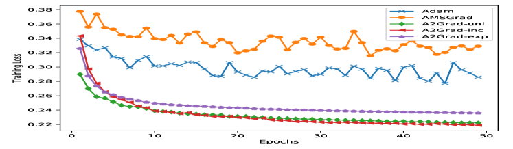
(a)

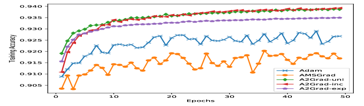
(b)

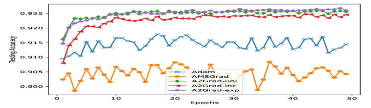
(c)

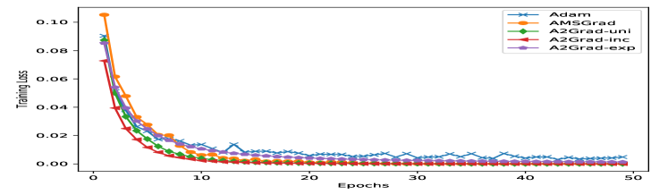
(d)

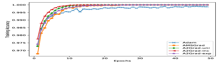
(e)

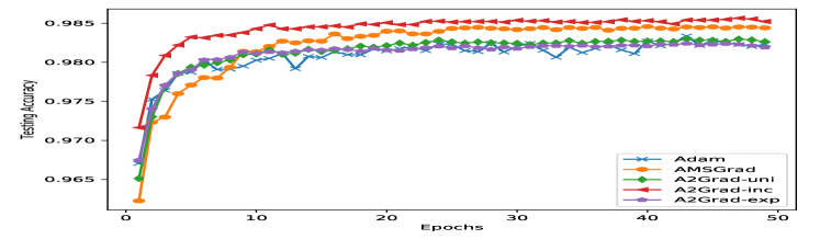
(f)

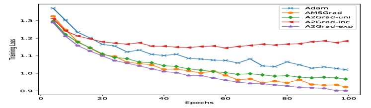
(g)

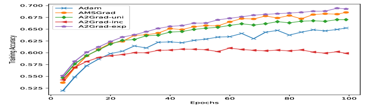
(h)

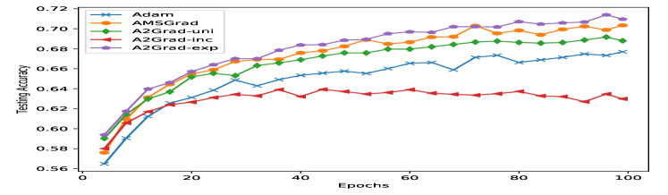
(i)

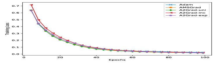
(j)

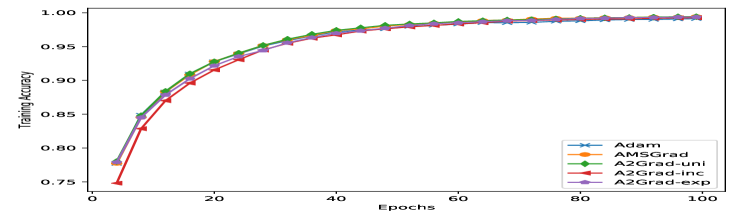
(k)

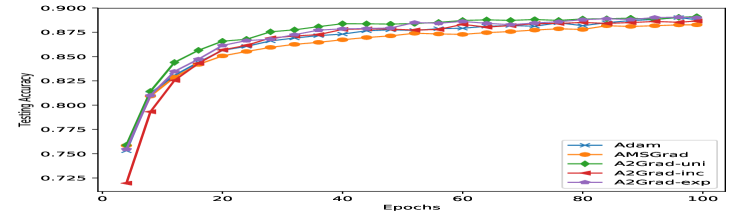
(l)

Figure 1: Comparison of algorithm performance on convex and nonconvex models. From left to right, each column represents the training loss, training accuracy and test accuracy. The first and second row plot the experimental results for logistic regression and neural network on the MNIST dataset respectively. The third and fourth rows plot the results for Cifarnet and Vgg16 on CIFAR10 respectively.

6 Conclusion

This paper develops a new framework of accelerated stochastic gradient methods with new adaptive gradients and moving average schemes. The primary goal is to tackle the issue of existing adaptive methods and develop more efficient adaptive accelerated methods. In contrast to the earlier work on adaptive methods, we provide novel analysis to decompose the complexity contributed by adaptive gradients and Nesterov’s momentum. Our theory gives new insight to the interplay of adaptive gradient and momentum and inspires us to design new adaptive diagonal function. By choosing adaptive function properly, we further develop new schemes of moving average—incorporating uniform average and exponential average but providing more—with unified theoretical convergence analysis. Our proposed algorithms not only achieve the optimal worst case complexity rates with respect to both the momentum part and stochastic part, but also demonstrate their empirical advantage over state of the art adaptive methods through experiments on both convex and nonconvex problems.

Appendix

Proof of Theorems

Before proving Theorem 1, we present a version of the three-point Lemma as follows:

Lemma 1.

Let $\phi$ and $\psi$ be two proximal functions and

$$z=\operatornamewithlimits{argmin}_{x\in\mathcal{X}}\{\langle g,x\rangle+\alpha D_{\phi}(y_{1},x)+\beta D_{\psi}(y_{2},x)\}.$$

Then $\forall x\in\mathcal{X}$, one has

$$\langle g,z\rangle+\alpha D_{\phi}(y_{1},z)+\beta D_{\psi}(y_{2},z)\leq\langle g,x\rangle+\alpha D_{\phi}(y_{1},x)+\beta D_{\psi}(y_{2},x)-\alpha D_{\phi}(z,x)-\beta D_{\psi}(z,x).$$

See 1

Proof.

First let us denote $g_{k}=\nabla f(\underline{x}_{k})$ for simplicity, we have

$$f(\bar{x}_{k+1}) \leq f(\underline{x}_{k})+\left\langle g_{k},\bar{x}_{k+1}-\underline{x}_{k}\right\rangle+\frac{L}{2}\|\bar{x}_{k+1}-\underline{x}_{k}\|^{2}$$

$$=f(\underline{x}_{k})+(1-\alpha_{k})\left\langle g_{k},\bar{x}_{k}-\underline{x}_{k}\right\rangle$$

$$+\alpha_{k}\left\langle g_{k},x_{k+1}-\underline{x}_{k}\right\rangle+\frac{L\alpha_{k}^{2}}{2}\|x_{k+1}-x_{k}\|^{2}$$

$$\leq(1-\alpha_{k})f(\bar{x}_{k})+\alpha_{k}[f(\underline{x}_{k})+\left\langle\underline{G}_{k},x_{k+1}-\underline{x}_{k}\right\rangle]$$

$$+\frac{L\alpha_{k}^{2}}{2}\|x_{k+1}-x_{k}\|^{2}-\alpha_{k}\left\langle\delta{}_{k},x_{k+1}-\underline{x}_{k}\right\rangle$$ (13)

In light of Lemma 1, we obtain the mirror descent step:

$$\left\langle\underline{G}_{k},x_{k+1}-\underline{x}_{k}\right\rangle\leq\left\langle\underline{G}_{k},x-\underline{x}_{k}\right\rangle+\gamma_{k}\{D(x_{k},x)-D(x_{k+1},x)-D(x_{k},x_{k+1})\}+\beta_{k}\{D_{\phi_{k}}(x_{k},x)-D_{\phi_{k}}(x_{k+1},x)-D_{\phi_{k}}(x_{k},x_{k+1})\}$$ (14)

Next applying convexity of $f(x)$, we have

$$f(\underline{x}_{k})+\left\langle\underline{G}_{k},x-\underline{x}_{k}\right\rangle =f(\underline{x}_{k})+\left\langle g_{k},x-\underline{x}_{k}\right\rangle+\left\langle\delta_{k},x-\underline{x}_{k}\right\rangle$$

$$\leq f(x)+\left\langle\delta_{k},x-\underline{x}_{k}\right\rangle.$$ (15)

Putting (13), (14) and (15) together, we arrive at

$$f(\bar{x}_{k+1}) \leq(1-\alpha_{k})f(\bar{x}_{k})+\alpha_{k}f(x)-\frac{1}{2}(\alpha_{k}\gamma_{k}-L\alpha_{k}^{2})\|x_{k+1}-x_{k}\|^{2}$$

$$\quad+\alpha_{k}\gamma_{k}\{D(x_{k},x)-D(x_{k+1},x)\}+\alpha_{k}\beta_{k}\left\{D_{\phi_{k}}(x_{k},x)-D_{\phi_{k}}(x_{k+1},x)\right\}$$

$$\quad+\alpha_{k}\langle\delta_{k},x_{k}-x_{k+1}\rangle-\alpha_{k}\beta_{k}D_{\phi_{k}}(x_{k},x_{k+1})$$

$$\quad+\alpha_{k}\left\langle\delta_{k},x-x_{k}\right\rangle$$

$$\leq(1-\alpha_{k})f(\bar{x}_{k})+\alpha_{k}f(x)-\frac{1}{2}\alpha_{k}\beta_{k}\|x_{k}-x_{k+1}\|^{2}_{\phi_{k}}$$

$$\quad+\alpha_{k}\langle\delta_{k},x_{k}-x_{k+1}\rangle+\alpha_{k}\langle\delta_{k},x-x_{k}\rangle$$

$$\quad+\alpha_{k}\gamma_{k}\{D(x_{k},x)-D(x_{k+1},x)\}+\alpha_{k}\beta_{k}\left\{D_{\phi_{k}}(x_{k},x)-D_{\phi_{k}}(x_{k+1},x)\right\}$$

$$\leq(1-\alpha_{k})f(\bar{x}_{k})+\alpha_{k}f(x)-\frac{1}{2}\alpha_{k}\beta_{k}\|x_{k}-x_{k+1}\|^{2}_{\phi_{k}}$$

$$\quad+\alpha_{k}\|\delta_{k}\|_{\phi_{k}^{*}}\|x_{k}-x_{k+1}\|_{\phi_{k}}+\alpha_{k}\langle\delta_{k},x-x_{k}\rangle$$

$$\quad+\alpha_{k}\gamma_{k}\{D(x_{k},x)-D(x_{k+1},x)\}+\alpha_{k}\beta_{k}\left\{D_{\phi_{k}}(x_{k},x)-D_{\phi_{k}}(x_{k+1},x)\right\}$$

$$\leq(1-\alpha_{k})f(\bar{x}_{k})+\alpha_{k}f(x)+\alpha_{k}\|\delta_{k}\|_{\phi_{k}*}^{2}/(2\beta_{k})$$

$$\quad+\alpha_{k}\gamma_{k}\{D(x_{k},x)-D(x_{k+1},x)\}+\alpha_{k}\beta_{k}\left\{D_{\phi_{k}}(x_{k},x)-D_{\phi_{k}}(x_{k+1},x)\right\}$$

$$\quad+\alpha_{k}\left\langle\delta_{k},x-x_{k}\right\rangle.$$

red In the first and second inequalities we use the strong convexity of proximal functions: $D(x,y)\geq\frac{1}{2}\|x-y\|^{2}$ and $D_{\phi_{k}}(x,y)\geq\frac{1}{2}\|x-y\|^{2}_{\phi_{k}}$ and the fact that $-\frac{1}{2}(\alpha_{k}\gamma_{k}-L\alpha_{k}^{2})\|x_{k}-x_{k+1}\|^{2}\leq 0$ by the relation (5); in the third inequality, we apply Cauchy–Schwarz inequality as $\langle\delta_{k},x_{k}-x_{k+1}\rangle\leq\|\delta_{k}\|_{\phi_{k}^{*}}\cdot\|x_{k}-x_{k+1}\|_{\phi_{k}}$; in the last inequality, we use the fact that for $a>0$, $bx-\frac{a}{2}x^{2}\leq\frac{b^{2}}{2a}$.

Finally, summing up the above relation for $k=0,1,2,...$ with each side weighted by $\lambda_{k}$, and using relation (6), we have

$$\lambda_{K}\left[f(\bar{x}_{K+1})-f(x)\right]\leq(1-\alpha_{0})\left[f(\bar{x}_{0})-f(x)\right]+\alpha_{0}\gamma_{0}D(x_{0},x)+\sum_{k=0}^{K}\lambda_{k}[\frac{\alpha_{k}\|\delta_{k}\|_{\phi_{k}*}^{2}}{2\beta_{k}}+\alpha_{k}\left\langle\delta_{k},x-x_{k}\right\rangle+\alpha_{k}R_{k}],$$ (16)

where $R_{k}=\beta_{k}D_{\phi_{k}}(x_{k},x)-\beta_{k}D_{\phi_{k}}(x_{k+1},x).$ ∎

See 2

Proof.

One has

$$\sum_{k=0}^{K}\lambda_{k}\alpha_{k}\left\{\beta_{k}D_{\phi_{k}}(x_{k},x)-\beta_{k}D_{\phi_{k}}(x_{k+1},x)\right\}$$

$${\leq} \sum_{k=1}^{K}\left[\lambda_{k}\alpha_{k}\beta_{k}D_{\phi_{k}}(x_{k},x)-\lambda_{k-1}\alpha_{k-1}\beta_{k-1}D_{\phi_{k-1}}(x_{k},x)\right]$$

$$+\lambda_{0}\alpha_{0}\beta_{0}D_{\phi_{0}}(x_{0},x)$$

$$\overset{\text{(\ref{monotone})}}{\leq} \sum_{k=1}^{K}\sum_{i=1}^{d}\left[\lambda_{k}\alpha_{k}\beta_{k}h_{k,i}-\lambda_{k-1}\alpha_{k-1}\beta_{k-1}h_{k-1,i}\right]B$$

$$+\lambda_{0}\alpha_{0}\beta_{0}\sum_{i=1}^{d}h_{0,i}B$$

$$\leq \lambda_{K}\alpha_{K}\beta_{K}\sum_{i=1}^{d}h_{K,i}B.$$

redMoreover, we have $\lambda_{k}=\frac{(k+1)(k+2)}{2}$ by the definition of $\alpha_{k}$, and $\mathbb{E}[\langle\delta_{k},x_{k}-x\rangle]=0$ by taking expectation w.r.t stochastic gradient $\underline{G}_{k}$. It then remains to plug in the values of $\alpha_{k}$ and $\lambda_{k}$ to (16) to prove our result. ∎

Proof of Corollaries

See 1 The proof of Corollary 1 is built on Lemma 10 in [4]. For the sake of convenience, we present this lemma as follows:

Lemma 2.

Let $\{a_{\tau}\}_{0\leq\tau\leq t}$ be a sequence of real values, and $a_{:\tau}=[a_{0},a_{1},...,a_{\tau}]^{T}$ , then

$$\sum_{\tau=0}^{t}\frac{a_{\tau}^{2}}{\|a_{:\tau}\|_{2}}\leq 2\|a_{:t}\|_{2}.$$

Proof of Corollary 1.

Define $\bar{\delta}_{k}=(k+1)^{q/2}\delta_{k}$. Using Lemma 2, we arrive at

$$\sum_{k=0}^{K}\frac{(k+1)\|\delta_{k}\|_{h_{k}*}^{2}}{\beta_{k}} =\sum_{k=0}^{K}\sum_{i=1}^{d}\frac{(k+1)\delta_{k,i}^{2}}{\beta h_{k,i}}$$

$$=\sum_{k=0}^{K}\sum_{i=1}^{d}\frac{(k+1)^{1-q/2}\bar{\delta}_{k,i}^{2}}{\beta\|\bar{\delta}_{:k,i}\|_{2}}$$

$$\leq\frac{2(K+1)^{1-q/2}}{\beta}\sum_{i=1}^{d}\|\bar{\delta}_{:k,i}\|.$$ (17)

Moreover, by the definition of $\bar{\delta}$, we have

$$\|\bar{\delta}_{:k,i}\|_{2}=\sqrt{\sum_{\tau=0}^{k}(\tau+1)^{q}\delta_{\tau,i}^{2}}\leq(k+1)^{q/2}\|\delta_{:k,i}\|_{2},\ 1\leq i\leq d.$$ (18)

This also gives rise to the bound $h_{k,i}\leq\|\delta_{0:k,i}\|_{2}$. Putting these together, we have

$$\mathbb{E}\left[f(\bar{x}_{K+1})-f(x)\right]\leq\frac{2L\|x-x_{0}\|^{2}}{(K+1)(K+2)}+\frac{2\beta B\ \mathbb{E}\left[\sum_{i=1}^{d}\|\delta_{0:K,i}\|\right]}{K+2}+\frac{2\mathbb{E}\left[\sum_{i=1}^{d}\|\delta_{0:K,i}\|\right]}{\beta(K+2)}$$

∎

See 2

Proof.

Using the definition of $h_{k},v_{k}$, we have

$$h_{k}\geq(1-\rho)\sqrt{k+1}\delta_{k},\quad k=0,1,2,...$$

and

$$h_{k,i}\leq\sqrt{k+1}\max_{0\leq\tau\leq k}\left|\delta_{\tau,i}\right|,\quad i=1,2,...,d,\ k=0,1,2,...$$

$$\sum_{k=0}^{K}\frac{\lambda_{k}\alpha_{k}\|\delta_{k}\|_{\phi_{k}*}^{2}}{2\beta_{k}} \leq\sum_{k=0}^{K}\sum_{i=1}^{d}\frac{\sqrt{k+1}\left|\delta_{k,i}\right|}{2\beta(1-\rho)}$$

$$\leq\frac{\sqrt{K+1}}{2\beta(1-\rho)}\sum_{i=1}^{d}\|\delta_{:k,i}\|_{1}.$$ (19)

In conclusion, we have

$$\mathbb{E}\left[f(\bar{x}_{K+1})-f(x)\right]\leq\frac{2L\|x-x_{0}\|^{2}}{(K+1)(K+2)}+\frac{2\beta B\sum_{i=1}^{d}\mathbb{E}\left[\max_{0\leq k\leq K}\left|\delta_{k,i}\right|\right]}{\sqrt{K+2}}+\frac{\sum_{i=1}^{d}\mathbb{E}\left[\|\delta_{0:K,i}\|_{1}\right]}{2\beta(1-\rho)\sqrt{K+1}(K+2)}.$$

For the second part, it suffices to show the expectation of some max-type random variables. For brevity, we use $\delta_{k,i}$ $\delta_{i}$ exchangeably. Under the sub-Gaussian assumption, the moment generating function of $\delta_{i}$—$M_{t}$ satisfies

$$M_{t}=\mathbb{E}e^{t|\delta_{i}|}\leq 2e^{t^{2}\bar{\sigma}^{2}/2},$$

for any $t>0$. Using some standard analysis, we have

$$\exp\mathbb{E}\left[t\max_{0\leq k\leq K}\left|\delta_{k,i}\right|\right] \leq\mathbb{E}\left[\exp\left(t\max_{0\leq k\leq K}\left|\delta_{k,i}\right|\right)\right]$$

$$=\mathbb{E}\left[\max_{0\leq k\leq K}\exp\left(t\left|\delta_{k,i}\right|\right)\right]$$

$$\leq\sum_{0\leq k\leq K}\mathbb{E}\left[\exp t\left|\delta_{k,i}\right|\right]$$

$$=(K+1)M_{t}$$

where the first inequality is from Jensen’s inequality. Taking logarithm on both sides yields

$$\mathbb{E}\left[\max_{0\leq k\leq K}\left|\delta_{k,i}\right|\right]\leq\frac{\log(2(K+1))+t^{2}\bar{\sigma}^{2}/2}{t},\quad\forall t.$$

Choosing $t=\frac{\sqrt{2\log(2(K+1))}}{\bar{\sigma}}$, we have

$$\mathbb{E}\left[\max_{0\leq k\leq K}\left|\delta_{k,i}\right|\right]\leq\sqrt{2\log(2(K+1))}\bar{\sigma}.$$

Moreover, by sub-Gaussian property, we have $\mathbb{E}|\delta_{i}|\leq\bar{\sigma}\sqrt{2\pi}$. Overall, we have

$$\mathbb{E}\left[f(\bar{x}_{K+1})-f(x)\right]=\frac{2L\|x-x_{0}\|^{2}}{(K+1)(K+2)}+2\beta B\frac{\sqrt{2\log(2(K+1))}\bar{\sigma}}{\sqrt{K+2}}+\frac{\sqrt{2\pi}d\bar{\sigma}}{2\beta(1-\rho)\sqrt{K+2}}.$$

For the last part, by assuming $\|G(x,\xi)\|_{\infty}\leq C$ we will have $\|\delta_{k}\|_{\infty}\leq 2C$, $0\leq k\leq K$. Immediately, we draw the conclusion by plugging into (10). ∎

References

• [1] N. Agarwal, Z. Allen-Zhu, B. Bullins, E. Hazan, and T. Ma. Finding approximate local minima faster than gradient descent. In Proceedings of the 49th Annual ACM SIGACT Symposium on Theory of Computing, pages 1195–1199. ACM, 2017.
• [2] Y. Carmon, J. C. Duchi, O. Hinder, and A. Sidford. Accelerated methods for non-convex optimization. arXiv preprint arXiv:1611.00756, 2016.
• [3] T. Dozat. Incorporating nesterov momentum into adam. In International Conference on Learning Representations, 2016.
• [4] J. C. Duchi, E. Hazan, and Y. Singer. Adaptive subgradient methods for online learning and stochastic optimization. The Journal of Machine Learning Research (JMLR), 12:2121–2159, 2011.
• [5] R. Ge, F. Huang, C. Jin, and Y. Yuan. Escaping from saddle points-online stochastic gradient for tensor decomposition. In Conference on Learning Theory, pages 797–842, 2015.
• [6] S. Ghadimi and G. Lan. Accelerated gradient methods for nonconvex nonlinear and stochastic programming. Mathematical Programming, 156(1-2):59–99, 2016.
• [7] P. Jain, S. M. Kakade, R. Kidambi, P. Netrapalli, and A. Sidford. Accelerating stochastic gradient descent. arXiv preprint arXiv:1704.08227, 2017.
• [8] N. S. Keskar and R. Socher. Improving generalization performance by switching from adam to sgd. arXiv preprint arXiv:1712.07628, 2017.
• [9] R. Kidambi, P. Netrapalli, P. Jain, and S. M. Kakade. On the insufficiency of existing momentum schemes for stochastic optimization. arXiv preprint arXiv:1803.05591, 2018.
• [10] D. P. Kingma and J. Ba. Adam: A method for stochastic optimization. International Conference on Learning Representations, 2015.
• [11] G. Lan. Convex optimization under inexact first-order information. Georgia Institute of Technology, 2009.
• [12] G. Lan. An optimal method for stochastic composite optimization. Mathematical Programming, 133(1-2):365–397, 2012.
• [13] J. D. Lee, M. Simchowitz, M. I. Jordan, and B. Recht. Gradient descent only converges to minimizers. In Conference on Learning Theory, pages 1246–1257, 2016.
• [14] A. Nemirovski, A. Juditsky, G. Lan, and A. Shapiro. Robust stochastic approximation approach to stochastic programming. SIAM Journal on Optimization, 19(4):1574–1609, 2009.
• [15] A. Nemirovski and D. B. Yudin. Problem complexity and method efficiency in optimization. John Wiley and Sons, 1983.
• [16] Y. Nesterov. A method of solving a convex programming problem with convergence rate $\mathcal{O}(1/k^{2})$. Soviet Mathematics Doklady, 27(2):372–376, 1983.
• [17] Y. Nesterov. Introductory lectures on convex optimization: A basic course, volume 87. Springer, 2003.
• [18] Y. Nesterov and B. T. Polyak. Cubic regularization of newton method and its global performance. Mathematical Programming, 108(1):177–205, 2006.
• [19] B. T. Polyak. Some methods of speeding up the convergence of iteration methods. USSR Computational Mathematics and Mathematical Physics, 4(5):1–17, 1964.
• [20] B. T. Polyak. New stochastic approximation type procedures. Automat. i Telemekh, 7(98-107):2, 1990.
• [21] B. T. Polyak and A. B. Juditsky. Acceleration of stochastic approximation by averaging. SIAM Journal on Control and Optimization, 30(4):838–855, 1992.
• [22] S. J. Reddi, S. Kale, and S. Kumar. On the convergence of adam and beyond. In International Conference on Learning Representations, 2018.
• [23] H. Robbins and S. Monro. A stochastic approximation method. The Annals of Mathematical Statistics, pages 400–407, 1951.
• [24] K. Simonyan and A. Zisserman. Very deep convolutional networks for large-scale image recognition. international conference on learning representations, 2015.
• [25] I. Sutskever, J. Martens, G. Dahl, and G. Hinton. On the importance of initialization and momentum in deep learning. In International conference on machine learning, pages 1139–1147, 2013.
• [26] T. Tieleman and G. Hinton. Lecture 6.5-rmsprop: Divide the gradient by a running average of its recent magnitude. COURSERA: Neural networks for machine learning, 4(2):26–31, 2012.
• [27] N. Tripuraneni, M. Stern, C. Jin, J. Regier, and M. I. Jordan. Stochastic cubic regularization for fast nonconvex optimization. arXiv preprint arXiv:1711.02838, 2017.
• [28] P. Tseng. On accelerated proximal gradient methods for convex-concave optimization. submitted to SIAM Journal on Optimization, 2008.
• [29] A. C. Wilson, R. Roelofs, M. Stern, N. Srebro, and B. Recht. The marginal value of adaptive gradient methods in machine learning. In Advances in Neural Information Processing Systems, pages 4151–4161, 2017.
• [30] M. D. Zeiler. Adadelta: an adaptive learning rate method. arXiv preprint arXiv:1212.5701, 2012.