Power and Level Robustness of A Composite Hypothesis Testing under Independent Non-Homogeneous Data

Abstract

Robust tests of general composite hypothesis under non-identically distributed observations is always a challenge. Ghosh and Basu (2018, Statistica Sinica, 28, 1133–1155) have proposed a new class of test statistics for such problems based on the density power divergence, but their robustness with respect to the size and power are not studied in detail. This note fills this gap by providing a rigorous derivation of power and level influence functions of these tests to theoretically justify their robustness. Applications to the fixed-carrier linear regression model are also provided with empirical illustrations.

1 Introduction and Background

Robust statistical inference based on non-homogeneous data is always a big challenge and the likelihood ratio test (LRT), the canonical tool in these situations, is highly sensitive in the presence of outliers. Literature of alternative robust tests for statistical hypotheses are limited beyond the identically distributed data, except for some particular cases like the fixed-carrier linear regression model, etc. Recently, Ghosh and Basu (2018) have developed a class of robust testing procedures under the general set-up of independent but non-homogeneous (INH) observations based on the robust estimator of Ghosh and Basu (2013).

Under the general INH set-up, we assume that the observations $Y_{1},\ldots,Y_{n}$ are independent but $Y_{i}\sim g_{i}$ for each $i$ where $g_{1},\ldots,g_{n}$ are potentially different densities with respect to some common dominating measure. A parametric family of densities ${\mathcal{F}}_{i,{\boldsymbol{\theta}}}=\{f_{i}(\cdot;{\boldsymbol{\theta}})|~{}{\boldsymbol{\theta}}\in\Theta\}$ is assumed to model $g_{i}$, for each $i=1,2,\ldots,n$, and our interest is to make inference about the common parameter $\boldsymbol{\theta}$. The most common application is the fixed-carrier regressions, where each $f_{i}(\cdot;{\boldsymbol{\theta}})$ is the (conditional) density of the response given the $i$-th (fixed) value of the covariates. In general, we denote by $G_{i}$ and $F_{i}(\cdot,{\boldsymbol{\theta}})$ the distribution functions of $g_{i}$ and $f_{i}(\cdot;{\boldsymbol{\theta}})$ respectively. Under this INH set-up, Ghosh and Basu (2013) have developed a general robust estimator of $\boldsymbol{\theta}$ using the density power divergence (DPD) of Basu et al. (1998); this DPD measure, having a tuning parameter $\tau$, is defined between densities $f_{1}$ and $f_{2}$ as

$$d_{\tau}(f_{1},f_{2})=\displaystyle\left\{\begin{array}[]{ll}\displaystyle\int\left[f_{2}^{1+\tau}-\left(1+\frac{1}{\tau}\right)f_{2}^{\tau}f_{1}+\frac{1}{\tau}f_{1}^{1+\tau}\right],&{\rm for}~{}\tau>0,\\ \displaystyle\int f_{1}\log(f_{1}/f_{2}),&{\rm for}~{}\tau=0.\end{array}\right.$$ (1)

Since there are $n$ different densities for INH set-up, Ghosh and Basu (2013) minimized the average DPD measure $\frac{1}{n}\sum_{i=1}^{n}d_{\tau}(\widehat{g}_{i}(.),f_{i}(.;{\boldsymbol{\theta}}))$ with respect to $\boldsymbol{\theta}\in\Theta$, where $\widehat{g}_{i}$ is an estimator of $g_{i}$ based on the empirical distribution function. This minimum DPD estimator (MDPDE) has high efficiency and robustness properties, controlled by $\tau$, and works well in different fixed-design regressions by Ghosh and Basu (2013, 2016) and Ghosh (2017a, b). At $\tau=0$, the MDPDE coincides with the maximum likelihood estimator (MLE). Using this MDPDE, Ghosh and Basu (2018) have developed a class of robust DPD based tests for both simple and composite hypotheses indexed by the same $\tau$; they coincide with the LRT at $\tau=0$ and provide its robust generalization at $\tau>0$ without significant loss in efficiency. However, their theoretical robustness properties need to be studied in greater detail, particularly for composite hypothesis testing problems, where no details about the size and power robustness are available.

Since the size and power are the two most important measures to study the performance of any test, in this paper, we present detailed analysis for such robustness issues for the composite hypothesis tests of Ghosh and Basu (2018). In particular, we study their power and level influence functions to justify their robustness with a concrete theory; this needs some non-trivial extensions of the corresponding results from simple hypothesis case. We also illustrate their applications in testing general linear hypothesis under a fixed-carrier linear regression model (LRM) with unknown error variance. Empirical results from an extensive simulation study second our theoretical robustness analyses.

We provide a brief description of the composite hypothesis tests from Ghosh and Basu (2018) in Section 2. Our main results about the level and power influence functions are provided in Section 3. Section 4 presents the application to the LRMs and numerical illustrations are given in Section 5. Concluding remarks are given in Section 6. All notations are given in A, whereas the required assumptions and some background results are presented in the Online Supplement for completeness.

2 DPD based Tests for Composite Hypotheses under the INH Set-up

Consider the INH set-up of Section 1 and the problem of testing the composite hypothesis of the form

$$H_{0}:{\boldsymbol{\theta}}\in\Theta_{0}~{}~{}~{}\mbox{ against }~{}~{}~{}~{}H_{1}:{\boldsymbol{\theta}}\notin\Theta_{0},$$ (2)

where $\Theta_{0}\subset\Theta$. In most applications, the (fixed) null parameter space $\Theta_{0}$ is defined in terms of $r$ independent restrictions, say $\boldsymbol{\upsilon}({\boldsymbol{\theta}})=\boldsymbol{0}_{r}$. Ghosh and Basu (2018) have proposed to test (2) by the DPD based test statistics

$$S_{\gamma}({{\boldsymbol{\theta}}_{n}^{\tau}},{\widetilde{{\boldsymbol{\theta}}}_{n}^{\tau}})=2\sum_{i=1}^{n}d_{\gamma}(f_{i}(.;{\boldsymbol{\theta}}_{n}^{\tau}),f_{i}(.;\widetilde{{\boldsymbol{\theta}}}_{n}^{\tau})),~{}~{}~{}\tau,\gamma\geq 0,$$ (3)

where ${\boldsymbol{\theta}}_{n}^{\tau}$ and $\widetilde{{\boldsymbol{\theta}}}_{n}^{\tau}$ are the MDPDE and the restricted MDPDE (RMDPDE) of $\boldsymbol{\theta}$ respectively; the RMDPDE has to be obtained by minimizing the average DPD measure only over $\boldsymbol{\theta}\in\Theta_{0}$ (See Results 1 and 2 in Online Supplement for their asymptotic distributions). Ghosh and Basu (2018) have shown that, in general, its asymptotic null distribution is a linear combination of (central) chi-square distributions (Result 3 in Online Supplement); some suitable approximations are also suggested for its critical values following Basu et al. (2013). Further, this DPD based test is consistent at any fixed alternative.

However, in terms of robustness, only the influence function (IF) of the test statistic have been discussed in Ghosh and Basu (2018). The statistical functional corresponding to the test statistics in (3) is defined as

$$S_{\gamma,\tau}(\underline{\mathbf{G}})=\sum_{i=1}^{n}d_{\gamma}(f_{i}(.;U_{\tau}(\underline{\mathbf{G}})),f_{i}(.;\widetilde{U}_{\tau}(\underline{\mathbf{G}}))),$$

where $\underline{\mathbf{G}}=(G_{1},\cdots,G_{n})$ and $U_{\tau}(\underline{\mathbf{G}})$ and $\widetilde{U}_{\tau}(\underline{\mathbf{G}})$ are the functionals corresponding to the MDPDE and the RMDPDE, respectively, defined as the minimizers of $\frac{1}{n}\sum_{i=1}^{n}d_{\tau}({g}_{i}(.),f_{i}(.;{\boldsymbol{\theta}}))$ with respect to $\boldsymbol{\theta}\in\Theta$ and $\boldsymbol{\theta}\in\Theta_{0}$. Consider contamination in all densities at the contamination points in $\mathbf{t}=(t_{1},\ldots,t_{n})$ respectively. When evaluating at the null distribution $\underline{\mathbf{G}}=\underline{\mathbf{F}}_{\theta_{0}}=\left(F_{1}(\cdot,\boldsymbol{\theta}_{0}),\ldots,F_{n}(\cdot,\boldsymbol{\theta}_{0})\right)$ with $\theta_{0}\in\Theta_{0}$, the first order IF of $S_{\gamma,\tau}$ is identically zero and the corresponding second order IF is (Ghosh and Basu, 2018)

$$\mathcal{IF}_{2}(\mathbf{t},S_{\gamma,\tau},\underline{\mathbf{F}}_{\theta_{0}})=n\cdot\boldsymbol{D}_{\tau}(\mathbf{t},\boldsymbol{\theta}_{0})^{T}\boldsymbol{A}_{n}^{\gamma}(\boldsymbol{\theta}_{0})\boldsymbol{D}_{\tau}(\mathbf{t},\boldsymbol{\theta}_{0}),$$ (4)

where $\boldsymbol{D}_{\tau}(\mathbf{t},\boldsymbol{\theta}_{0})=\left[\mathcal{IF}(\mathbf{t},\boldsymbol{U}_{\tau},\underline{\mathbf{F}}_{\theta_{0}})-\mathcal{IF}(\mathbf{t},\widetilde{\boldsymbol{U}}_{\tau},\underline{\mathbf{F}}_{\theta_{0}})\right]$, the difference between IFs of the MDPDE $\boldsymbol{U}_{\tau}$ and the RMDPDE $\widetilde{\boldsymbol{U}}_{\tau}$ at $\underline{\mathbf{F}}_{\theta_{0}}$. But, both these IFs are both bounded at $\tau>0$ for most parametric models; at $\tau=0$ the IF of the MDPDE (MLE) is unbounded but that of RMDPDE depends on the restrictions $\boldsymbol{\upsilon}=\boldsymbol{0}$. So the second order IF (4) of our test statistics is bounded whenever $\boldsymbol{D}_{\tau}(\mathbf{t},\boldsymbol{\theta}_{0})$ is bounded, i.e., the IFs of MDPDE and RMDPDE both are bounded or both diverge at the same rate; this holds for $\tau>0$ in most cases. At $\tau=0$, this new test coincides with the non-robust LRT having unbounded IF.

3 Power and Level Influence Functions

For a hypothesis testing procedure, it is not enough to study only the properties of the test statistics; the level and power are two basic components of hypothesis testing whose robustness is essential to fully justify a new robust test procedure. In this section, we study the theoretical robustness properties of the power and level of the DPD based test in (3); it is done through the examination of classical power influence functions (PIF) and level influence function (LIF).

The PIF and LIF of a test measure the effect of infinitesimal contamination on its power and level respectively. However, the DPD based test (3) is consistent at any fixed alternative (Ghosh and Basu, 2018) and hence its power against any fixed alternative is always one. Further, exact finite-sample power is much difficult to derive. So, we study the effect of contamination on its asymptotic power against a sequence of contiguous alternatives $H_{1,n}:{\boldsymbol{\theta}}={\boldsymbol{\theta}}_{n}$, where ${\boldsymbol{\theta}}_{n}={\boldsymbol{\theta}}_{0}+n^{-1/2}\boldsymbol{\Delta}$ with ${\boldsymbol{\theta}}_{0}\in\Theta_{0}$ and $\boldsymbol{\Delta}\in\mathbb{R}^{p}-\{\boldsymbol{0}_{p}\}$. Such a ${\boldsymbol{\theta}}_{0}$ must be a limit point of $\Theta_{0}$; we assume $\Theta_{0}$ to be closed ensuring the existence of such a sequence $\boldsymbol{\theta}_{n}\in\Theta$. Then, we consider the contamination over these contiguous alternatives in such a way that the contamination effect vanishes at the same rate as ${\boldsymbol{\theta}}_{n}\rightarrow{\boldsymbol{\theta}}_{0}$ when $n\rightarrow\infty$; this is necessary to make the neighborhood of the null and alternative hypotheses well separated (Hampel et al., 1986). Note that $\boldsymbol{\Delta}=\boldsymbol{0}$ yields the results associated with level of the test. Thus, assuming contamination in all densities as in the previous section, the contaminated distributions need to be defined as

$$\mathbf{\underline{F}}_{n,\epsilon,\mathbf{t}}^{P}=\left(1-\frac{\epsilon}{\sqrt{n}}\right)\mathbf{\underline{F}}_{{\boldsymbol{\theta}}_{n}}+\frac{\epsilon}{\sqrt{n}}\wedge_{\mathbf{t}},\mbox{ and }\mathbf{\underline{F}}_{n,\epsilon,\mathbf{t}}^{L}=\left(1-\frac{\epsilon}{\sqrt{n}}\right)\mathbf{\underline{F}}_{{\boldsymbol{\theta}}_{0}}+\frac{\epsilon}{\sqrt{n}}\wedge_{\mathbf{t}},$$

for studying the stability of power and level respectively, where $\epsilon$ is the contamination proportion and $\wedge_{\mathbf{t}}=(\wedge_{{t}_{1}},\ldots,\wedge_{{t}_{n}})$ with $\wedge_{{t}_{i}}$ being the degenerate distribution at $t_{i}$ for each $i=1,\ldots,n$. Then the PIF and LIF of the test in (3), at the significance level $\alpha$, are defined, see Hampel et al. (1986), as

$$PIF(\mathbf{t};S_{\gamma,\tau},\mathbf{\underline{F}}_{{\boldsymbol{\theta}}_{0}}) = \lim_{n\rightarrow\infty}~{}\frac{\partial}{\partial\epsilon}P_{\mathbf{\underline{F}}_{n,\epsilon,\mathbf{t}}^{P}}(S_{\gamma}({{\boldsymbol{\theta}}_{n}^{\tau}},\widetilde{{\boldsymbol{\theta}}}_{n}^{\tau})>s_{\alpha}^{\tau,\gamma})\big{|}_{\epsilon=0},$$

$$LIF(\mathbf{t};S_{\gamma,\tau},\mathbf{\underline{F}}_{{\boldsymbol{\theta}}_{0}}) = \lim_{n\rightarrow\infty}~{}\frac{\partial}{\partial\epsilon}P_{\mathbf{\underline{F}}_{n,\epsilon,\mathbf{t}}^{L}}(S_{\gamma}({{\boldsymbol{\theta}}_{n}^{\tau}},\widetilde{{\boldsymbol{\theta}}}_{n}^{\tau})>s_{\alpha}^{\tau,\gamma})\big{|}_{\epsilon=0},$$

where $s_{\alpha}^{\tau,\gamma}$ is the $(1-\alpha)$-th quantile of the asymptotic null distribution of $S_{\gamma}({{\boldsymbol{\theta}}_{n}^{\tau}},\widetilde{{\boldsymbol{\theta}}}_{n}^{\tau})$. Ghosh and Basu (2018) have discussed these LIF and PIF for testing the simple null hypothesis; further applications can be found in Huber-Carol (1970), Heritier and Ronchetti (1994) and Toma and Broniatowski (2010) for both types of hypotheses. Following the same line of arguments, we start with the derivation of the asymptotic power of the DPD based test (3) under $\mathbf{\underline{F}}_{n,\epsilon,\mathbf{y}}^{P}$, recalling the notations from A.

Theorem 3.1.

Suppose that Assumptions (A1)-(A10), given in Online Supplement, hold at $\boldsymbol{\theta}=\boldsymbol{\theta}_{0}$ under the INH set-up. Then, for any $\boldsymbol{\Delta}\in\mathbb{R}^{p}$, $\epsilon\geq 0$, we have the following results.

1. Under $\mathbf{\underline{F}}_{n,\epsilon,\mathbf{t}}^{P}$, $S_{\gamma}({{\boldsymbol{\theta}}_{n}^{\tau}},{\widetilde{{\boldsymbol{\theta}}}_{n}^{\tau}})\displaystyle\mathop{\rightarrow}^{\mathcal{D}}\boldsymbol{W}^{T}\boldsymbol{A}_{\gamma}(\theta_{0})\boldsymbol{W}$, where $\boldsymbol{W}\sim N_{p}\left(\widetilde{\boldsymbol{\Delta}^{*}},\widetilde{\boldsymbol{\Sigma}}_{\tau}(\boldsymbol{\theta}_{0})\right)$ with $\widetilde{\boldsymbol{\Delta}^{*}}=\left[\boldsymbol{\Delta}+\epsilon\boldsymbol{D}_{\tau}(\mathbf{t},\boldsymbol{\theta}_{0})\right]$.

2. Suppose the $r$ eigenvalues of ${\boldsymbol{A}_{\gamma}}({\boldsymbol{\theta}}_{0})\widetilde{\boldsymbol{\Sigma}}_{\tau}({\boldsymbol{\theta}}_{0})$ are denoted as $\widetilde{\zeta_{1}^{\gamma,\tau}}({\boldsymbol{\theta}}_{0})$, $\ldots$, $\widetilde{\zeta_{r}^{\gamma,\tau}}({\boldsymbol{\theta}}_{0})$ with the corresponding normalized eigenvector matrix being $\widetilde{\boldsymbol{P}}_{\tau,\gamma}(\theta_{0})$. Denote $\widetilde{\boldsymbol{P}}_{\tau,\gamma}(\boldsymbol{\theta}_{0})\widetilde{\boldsymbol{\Sigma}}_{\tau}^{-1/2}(\boldsymbol{\theta}_{0})\widetilde{\boldsymbol{\Delta}^{*}}=\left({\widetilde{\delta}_{1}},\ldots,{\widetilde{\delta}_{p}}\right)^{T}.$ Then, the asymptotic distribution in (i) is also the distribution of $\sum\limits_{i=1}^{r}\widetilde{\zeta_{i}^{\gamma,\tau}}(\theta_{0})\chi_{1,\widetilde{\delta}_{i}}^{2}$, where $\chi_{1,\widetilde{\delta}_{i}^{2}}^{2}$s are independent non-central chi-square variables with degrees of freedom (df) $1$ and non-centrality parameter (ncp) $\widetilde{\delta}_{i}^{2}$ respectively, for $i=1,\ldots,r$.

3. The asymptotic power of the DPD based test (3) under $\mathbf{\underline{F}}_{n,\epsilon,\mathbf{t}}^{P}$ is given by

   $$P_{\tau,\gamma}^{*}(\boldsymbol{\Delta},\epsilon;\alpha) = \lim_{n\rightarrow\infty}P_{\mathbf{\underline{F}}_{n,\epsilon,\mathbf{t}}^{P}}\left(S_{\gamma}({\theta_{n}^{\tau}},\widetilde{\theta}_{n}^{\tau})>s_{\alpha}^{\tau,\gamma}\right)=\sum\limits_{v=0}^{\infty}~{}\widetilde{C_{v}^{\gamma,\tau}}(\boldsymbol{\theta}_{0},\widetilde{\boldsymbol{\Delta}^{*}})P\left(\chi_{r+2v}^{2}>{s_{\alpha}^{\tau,\gamma}}/{\widetilde{\zeta_{(1)}^{\gamma,\tau}}(\boldsymbol{\theta}_{0})}\right),$$

   where $\widetilde{\zeta_{(1)}^{\gamma,\tau}}(\boldsymbol{\theta}_{0})=\min\limits_{1\leq r\leq r}\widetilde{\zeta_{i}^{\gamma,\tau}}(\boldsymbol{\theta}_{0})$, $\chi_{r+2v}^{2}$ are independent chi-squares with df $r+2v$ for $v\geq 0$, and

   $$\widetilde{C_{v}^{\gamma,\tau}}(\boldsymbol{\theta}_{0},\widetilde{\boldsymbol{\Delta}^{*}})=\frac{1}{v!}\left(\prod\limits_{j=1}^{r}\frac{\widetilde{\zeta_{(1)}^{\gamma,\tau}}(\boldsymbol{\theta}_{0})}{\widetilde{\zeta_{j}^{\gamma,\tau}}(\boldsymbol{\theta}_{0})}\right)^{1/2}e^{-\frac{1}{2}\sum\limits_{j=1}^{r}\widetilde{\delta}_{j}^{2}}E(\widetilde{Q}^{v}),$$

   $$\mbox{with }~{}~{}~{}~{}~{}~{}~{}~{}~{}\widetilde{Q}=\frac{1}{2}\sum\limits_{j=1}^{r}\left[\left(1-\frac{\widetilde{\zeta_{(1)}^{\gamma,\tau}}(\boldsymbol{\theta}_{0})}{\widetilde{\zeta_{j}^{\gamma,\tau}}(\boldsymbol{\theta}_{0})}\right)^{1/2}Z_{j}+{\widetilde{\delta}_{j}}\left(\frac{\widetilde{\zeta_{(1)}^{\gamma,\tau}}(\boldsymbol{\theta}_{0})}{\widetilde{\zeta_{j}^{\gamma,\tau}}(\boldsymbol{\theta}_{0})}\right)^{1/2}\right]^{2},$$

   for $r$ independent standard normal random variables $Z_{1},\ldots,Z_{r}$.

Proof All notations and matrices used in this proof are defined in A for brevity. Let us denote ${\boldsymbol{\theta}}_{n}^{*}=\boldsymbol{U}_{\tau}(\mathbf{\underline{F}}_{n,\epsilon,\mathbf{t}}^{P})$ and $\widetilde{{\boldsymbol{\theta}}_{n}^{*}}=\widetilde{\boldsymbol{U}}_{\tau}(\mathbf{\underline{F}}_{n,\epsilon,\mathbf{t}}^{P})$. Fix any $i=1,\ldots,n$. We consider the second order Taylor series expansion of $d_{\gamma}(f_{i}(\cdot;{\boldsymbol{\theta}}),f_{i}(\cdot;\widetilde{{\boldsymbol{\theta}}}_{n}^{\tau}))$ around ${\boldsymbol{\theta}}={\boldsymbol{\theta}}_{n}^{*}$ at ${\boldsymbol{\theta}}={\boldsymbol{\theta}}_{n}^{\tau}$ as,

$$d_{\gamma}(f_{i}(\cdot;{\boldsymbol{\theta}}_{n}^{\tau}),f_{i}(\cdot;\widetilde{{\boldsymbol{\theta}}}_{n}^{\tau}))=d_{\gamma}(f_{i}(\cdot;{\boldsymbol{\theta}}_{n}^{*}),f_{i}(\cdot;\widetilde{{\boldsymbol{\theta}}}_{n}^{\tau}))+\boldsymbol{M}_{1,\gamma}^{(i)}({\boldsymbol{\theta}}_{n}^{*},\widetilde{{\boldsymbol{\theta}}}_{n}^{\tau})^{T}({\boldsymbol{\theta}}_{n}^{\tau}-{\boldsymbol{\theta}}_{n}^{*})$$

$$~{}~{}~{}~{}~{}~{}~{}~{}~{}~{}~{}~{}~{}~{}~{}~{}+\frac{1}{2}({\boldsymbol{\theta}}_{n}^{\tau}-{\boldsymbol{\theta}}_{n}^{*})^{T}\boldsymbol{A}_{1,1,\gamma}^{(i)}({\boldsymbol{\theta}}_{n}^{*},\widetilde{{\boldsymbol{\theta}}}_{n}^{\tau})({\boldsymbol{\theta}}_{n}^{\tau}-{\boldsymbol{\theta}}_{n}^{*})+o(||{\boldsymbol{\theta}}_{n}^{\tau}-{\boldsymbol{\theta}}_{n}^{*}||^{2}).~{}~{}~{}~{}~{}~{}$$ (5)

Now, using Result 1 of Online Supplement and the consistency of ${\boldsymbol{\theta}}_{n}^{*}$ we know that, under $\mathbf{\underline{F}}_{n,\epsilon,\mathbf{t}}^{P}$, $\sqrt{n}({\boldsymbol{\theta}}_{n}^{\tau}-{\boldsymbol{\theta}}_{n}^{*})\mathop{\rightarrow}^{\mathcal{D}}N_{p}(\boldsymbol{0},\boldsymbol{J}_{\tau}^{-1}({\boldsymbol{\theta}}_{0})\boldsymbol{V}_{\tau}({\boldsymbol{\theta}}_{0})\boldsymbol{J}_{\tau}^{-1}({\boldsymbol{\theta}}_{0})).$ Further Taylor series expansions around ${\boldsymbol{\theta}}=\widetilde{{\boldsymbol{\theta}}_{n}^{*}}$ at ${\boldsymbol{\theta}}=\widetilde{{\boldsymbol{\theta}}}_{n}^{\tau}$ lead to

$$d_{\gamma}(f_{i}(\cdot;{\boldsymbol{\theta}}_{n}^{*}),f_{i}(\cdot;\widetilde{{\boldsymbol{\theta}}}_{n}^{\tau}))=d_{\gamma}(f_{i}(\cdot;{\boldsymbol{\theta}}_{n}^{*}),f_{i}(\cdot;\widetilde{{\boldsymbol{\theta}}_{n}^{*}}))+\boldsymbol{M}_{2,\gamma}^{(i)}({\boldsymbol{\theta}}_{n}^{*},\widetilde{{\boldsymbol{\theta}}_{n}^{*}})^{T}(\widetilde{{\boldsymbol{\theta}}}_{n}^{\tau}-\widetilde{{\boldsymbol{\theta}}_{n}^{*}})$$

$$~{}~{}~{}~{}~{}~{}~{}~{}~{}~{}~{}~{}+\frac{1}{2}(\widetilde{{\boldsymbol{\theta}}}_{n}^{\tau}-\widetilde{{\boldsymbol{\theta}}_{n}^{*}})^{T}\boldsymbol{A}_{2,2,\gamma}^{(i)}({{\boldsymbol{\theta}}}_{n}^{*},\widetilde{{\boldsymbol{\theta}}_{n}^{*}})(\widetilde{{\boldsymbol{\theta}}}_{n}^{\tau}-\widetilde{{\boldsymbol{\theta}}_{n}^{*}})+o(||\widetilde{{\boldsymbol{\theta}}}_{n}^{\tau}-\widetilde{{\boldsymbol{\theta}}_{n}^{*}}||^{2}),$$

$$\boldsymbol{M}_{1,\gamma}^{(i)}({\boldsymbol{\theta}}_{n}^{*},\widetilde{{\boldsymbol{\theta}}}_{n}^{\tau})=\boldsymbol{M}_{1,\gamma}^{(i)}({\boldsymbol{\theta}}_{n}^{*},\widetilde{{\boldsymbol{\theta}}_{n}^{*}})+\boldsymbol{A}_{2,1,\gamma}^{(i)}({{\boldsymbol{\theta}}}_{n}^{*},\widetilde{{\boldsymbol{\theta}}_{n}^{*}})(\widetilde{{\boldsymbol{\theta}}}_{n}^{\tau}-\widetilde{{\boldsymbol{\theta}}_{n}^{*}})+o(||\widetilde{{\boldsymbol{\theta}}}_{n}^{\tau}-\widetilde{{\boldsymbol{\theta}}_{n}^{*}}||),$$

and $\boldsymbol{A}_{1,1,\gamma}^{(i)}({\boldsymbol{\theta}}_{n}^{*},\widetilde{{\boldsymbol{\theta}}}_{n}^{\tau})=\boldsymbol{A}_{1,1,\gamma}^{(i)}({{\boldsymbol{\theta}}}_{n}^{*},\widetilde{{\boldsymbol{\theta}}_{n}^{*}})+o_{P}(1)$. Again, for each $j=1,2$, Taylor series expansion of $\boldsymbol{M}_{j,\gamma}^{(i)}({\boldsymbol{\theta}},\widetilde{{\boldsymbol{\theta}}_{n}^{*}})$ around ${\boldsymbol{\theta}}={\boldsymbol{\theta}}_{0}$ at ${\boldsymbol{\theta}}={\boldsymbol{\theta}}_{n}^{*}$ gives

$$\boldsymbol{M}_{j,\gamma}^{(i)}({\boldsymbol{\theta}}_{n}^{*},\widetilde{{\boldsymbol{\theta}}_{n}^{*}}) = \boldsymbol{M}_{j,\gamma}^{(i)}({\boldsymbol{\theta}}_{0},\widetilde{{\boldsymbol{\theta}}_{n}^{*}})+\frac{1}{\sqrt{n}}\boldsymbol{A}_{1,j,\gamma}^{(i)}({\boldsymbol{\theta}}_{0},\widetilde{{\boldsymbol{\theta}}_{n}^{*}}){\boldsymbol{\Delta}}+\frac{\epsilon}{\sqrt{n}}\boldsymbol{A}_{1,j,\gamma}^{(i)}({\boldsymbol{\theta}}_{0},\widetilde{{\boldsymbol{\theta}}_{n}^{*}})\mathcal{IF}(\mathbf{t};\boldsymbol{U}_{\tau},\mathbf{\underline{F}}_{{\boldsymbol{\theta}}_{0}})+o\left(\frac{1}{\sqrt{n}}\right)$$

$$= \boldsymbol{M}_{j,\gamma}^{(i)}({\boldsymbol{\theta}}_{0},\widetilde{{\boldsymbol{\theta}}_{n}^{*}})+\frac{1}{\sqrt{n}}\boldsymbol{A}_{1,j,\gamma}^{(i)}({\boldsymbol{\theta}}_{0},\widetilde{{\boldsymbol{\theta}}_{n}^{*}})\widetilde{{\boldsymbol{\Delta}}_{1}}+o\left(\frac{1}{\sqrt{n}}\right),$$

where $\widetilde{{\boldsymbol{\Delta}}_{1}}={\boldsymbol{\Delta}}+\epsilon\mathcal{IF}(\mathbf{t};\boldsymbol{U}_{\tau},\mathbf{\underline{F}}_{{\boldsymbol{\theta}}_{0}})$. For each $j,k=1,2$ and $i=1,\ldots,n$, similar use of suitable Taylor series expansions yield $\boldsymbol{A}_{j,k,\gamma}^{(i)}({{\boldsymbol{\theta}}}_{n}^{*},\widetilde{{\boldsymbol{\theta}}_{n}^{*}})=\boldsymbol{A}_{1,1,\gamma}^{(i)}({{\boldsymbol{\theta}}}_{0},\widetilde{{\boldsymbol{\theta}}_{n}^{*}})+o(1)=\boldsymbol{A}_{1,1,\gamma}^{(i)}({{\boldsymbol{\theta}}}_{n}^{*},{\boldsymbol{\theta}}_{0})+o(1)$, and

$$\boldsymbol{M}_{j,\gamma}^{(i)}({\boldsymbol{\theta}}_{0},\widetilde{{\boldsymbol{\theta}}_{n}^{*}}) = \boldsymbol{M}_{j,\gamma}^{(i)}({\boldsymbol{\theta}}_{0},{{\boldsymbol{\theta}}_{0}})+\frac{\epsilon}{\sqrt{n}}\boldsymbol{A}_{2,j,\gamma}^{(i)}({\boldsymbol{\theta}}_{0},{\boldsymbol{\theta}}_{0})\mathcal{IF}(\mathbf{t};\widetilde{\boldsymbol{U}}_{\tau},\mathbf{\underline{F}}_{{\boldsymbol{\theta}}_{0}})+o\left(\frac{1}{\sqrt{n}}\right),$$

$$\boldsymbol{M}_{j,\gamma}^{(i)}({{\boldsymbol{\theta}}_{n}^{*}},{\boldsymbol{\theta}}_{0}) = \boldsymbol{M}_{j,\gamma}^{(i)}({\boldsymbol{\theta}}_{0},{{\boldsymbol{\theta}}_{0}})+\frac{1}{\sqrt{n}}\boldsymbol{A}_{1,j,\gamma}^{(i)}({\boldsymbol{\theta}}_{0},{\boldsymbol{\theta}}_{0})\widetilde{{\boldsymbol{\Delta}}_{1}}+o\left(\frac{1}{\sqrt{n}}\right).$$

Now, we use these expressions to simplify Equation (5) and consider its summation over all $i=1,\ldots,n$. But, we also know that ${{\boldsymbol{\theta}}}_{n}^{*}\rightarrow{\boldsymbol{\theta}}_{0}$ as $n\rightarrow\infty$ and so $\frac{1}{n}\sum\limits_{i=1}^{n}\boldsymbol{M}_{j,\gamma}^{(i)}({{\boldsymbol{\theta}}_{n}^{*}},{\boldsymbol{\theta}}_{0})\rightarrow\boldsymbol{M}_{\gamma}({\boldsymbol{\theta}}_{0})=\boldsymbol{0}$ and $\frac{1}{n}\sum\limits_{i=1}^{n}\boldsymbol{A}_{j,k,\gamma}^{(i)}({{\boldsymbol{\theta}}_{n}^{*}},{\boldsymbol{\theta}}_{0})\rightarrow(-1)^{j+k}\boldsymbol{A}_{\gamma}({\boldsymbol{\theta}}_{0})$ as $n\rightarrow\infty$ for all $j,k=1,2$. Thus, we get

$$\frac{1}{\sqrt{n}}\sum\limits_{i=1}^{n}\boldsymbol{M}_{j,\gamma}^{(i)}({\boldsymbol{\theta}}_{n}^{*},\widetilde{{\boldsymbol{\theta}}_{n}^{*}}) = (-1)^{1+j}\boldsymbol{A}_{\gamma}({\boldsymbol{\theta}}_{0})\left[\widetilde{{\boldsymbol{\Delta}}_{1}}-\epsilon\mathcal{IF}(\mathbf{t};\widetilde{\boldsymbol{U}}_{\tau},\mathbf{\underline{F}}_{{\boldsymbol{\theta}}_{0}})\right]+o\left(1\right)=(-1)^{1+j}\boldsymbol{A}_{\gamma}({\boldsymbol{\theta}}_{0})\widetilde{{\boldsymbol{\Delta}}^{*}}+o\left(1\right),$$

where $\widetilde{{\boldsymbol{\Delta}}^{*}}$ is as defined in the theorem. Next, another Taylor series expansion of $d_{\gamma}(f_{i}(\cdot;{\boldsymbol{\theta}}_{n}^{*}),f_{i}(\cdot;{\boldsymbol{\theta}}))$ around ${\boldsymbol{\theta}}={\boldsymbol{\theta}}_{0}$ at ${\boldsymbol{\theta}}=\widetilde{{\boldsymbol{\theta}}_{n}^{*}}$ gives

$$d_{\gamma}(f_{i}(\cdot;{\boldsymbol{\theta}}_{n}^{*}),f_{i}(\cdot;\widetilde{{\boldsymbol{\theta}}_{n}^{*}})) = d_{\gamma}(f_{i}(\cdot;{\boldsymbol{\theta}}_{n}^{*}),f_{i}(\cdot;{{\boldsymbol{\theta}}}_{0}))+\frac{\epsilon}{\sqrt{n}}\boldsymbol{M}_{2,\gamma}^{(i)}({\boldsymbol{\theta}}_{n}^{*},{\boldsymbol{\theta}}_{0})\mathcal{IF}(\mathbf{t};\widetilde{\boldsymbol{U}}_{\tau},\mathbf{\underline{F}}_{{\boldsymbol{\theta}}_{0}})$$

$$+\frac{\epsilon^{2}}{2n}\mathcal{IF}(\mathbf{t};\widetilde{\boldsymbol{U}}_{\tau},\mathbf{\underline{F}}_{{\boldsymbol{\theta}}_{0}})^{T}\boldsymbol{A}_{2,2,\gamma}^{(i)}({\boldsymbol{\theta}}_{n}^{*},{\boldsymbol{\theta}}_{0})\mathcal{IF}(\mathbf{t};\widetilde{\boldsymbol{U}}_{\tau},\mathbf{\underline{F}}_{{\boldsymbol{\theta}}_{0}})+o\left(\frac{1}{n}\right).$$

$$\mbox{Similarly }~{}~{}2\sum_{i=1}^{n}d_{\gamma}(f_{i}(\cdot;{\boldsymbol{\theta}}_{n}^{*}),f_{i}(\cdot;{\boldsymbol{\theta}}_{0})) = {\boldsymbol{\Delta}}^{T}\boldsymbol{A}_{n}^{\gamma}({\boldsymbol{\theta}}_{0}){\boldsymbol{\Delta}}+2\epsilon{\boldsymbol{\Delta}}^{T}\boldsymbol{A}_{n}^{\gamma}({\boldsymbol{\theta}}_{0})\mathcal{IF}(\mathbf{t};\boldsymbol{U}_{\tau},\mathbf{\underline{F}}_{{\boldsymbol{\theta}}_{0}})$$

$$+ \epsilon^{2}\mathcal{IF}(\mathbf{t};\boldsymbol{U}_{\tau},\mathbf{\underline{F}}_{{\boldsymbol{\theta}}_{0}})\boldsymbol{A}_{n}^{\gamma}({\boldsymbol{\theta}}_{0})^{T}\mathcal{IF}(\mathbf{t};\boldsymbol{U}_{\tau},\mathbf{\underline{F}}_{{\boldsymbol{\theta}}_{0}})+o\left(1\right)$$

$$= \widetilde{{\boldsymbol{\Delta}}_{1}}^{T}\boldsymbol{A}_{n}^{\gamma}({\boldsymbol{\theta}}_{0})\widetilde{{\boldsymbol{\Delta}}_{1}}+o\left(1\right).$$

Combining last two equations, $2\sum_{i=1}^{n}d_{\gamma}(f_{i}(\cdot;{\boldsymbol{\theta}}_{n}^{*}),f_{i}(\cdot;\widetilde{{\boldsymbol{\theta}}_{n}^{*}}))=\widetilde{{\boldsymbol{\Delta}}^{*}}^{T}\boldsymbol{A}_{\gamma}({\boldsymbol{\theta}}_{0})\widetilde{{\boldsymbol{\Delta}}^{*}}+o\left(1\right)$. Therefore, noting that $n\times o(||{\boldsymbol{\theta}}_{n}^{\tau}-{\boldsymbol{\theta}}_{n}^{*}||^{2})=o_{P}(1)$ and $n\times o(||\widetilde{{\boldsymbol{\theta}}}_{n}^{\tau}-\widetilde{{\boldsymbol{\theta}}_{n}^{*}}||^{2})=o_{P}(1)$, we get the simplified expression as follows.

$$2\sum_{i=1}^{n}d_{\gamma}(f_{i}(\cdot;{\boldsymbol{\theta}}_{n}^{\tau}),f_{i}(\cdot;\widetilde{{\boldsymbol{\theta}}}_{n}^{\tau}))=\widetilde{{\boldsymbol{\Delta}}^{*}}^{T}\boldsymbol{A}_{n}^{\gamma}({\boldsymbol{\theta}}_{0})\widetilde{{\boldsymbol{\Delta}}^{*}}+2\widetilde{{\boldsymbol{\Delta}}^{*}}^{T}\boldsymbol{A}_{\gamma}({\boldsymbol{\theta}}_{0})\sqrt{n}({\boldsymbol{\theta}}_{n}^{\tau}-{\boldsymbol{\theta}}_{n}^{*})$$

$$- 2\widetilde{{\boldsymbol{\Delta}}^{*}}^{T}\boldsymbol{A}_{\gamma}({\boldsymbol{\theta}}_{0})\sqrt{n}(\widetilde{{\boldsymbol{\theta}}}_{n}^{\tau}-\widetilde{{\boldsymbol{\theta}}_{n}^{*}})+\sqrt{n}({\boldsymbol{\theta}}_{n}^{\tau}-{\boldsymbol{\theta}}_{n}^{*})^{T}\boldsymbol{A}_{\gamma}({\boldsymbol{\theta}}_{0})\sqrt{n}({\boldsymbol{\theta}}_{n}^{\tau}-{\boldsymbol{\theta}}_{n}^{*})$$

$$- 2\sqrt{n}(\widetilde{{\boldsymbol{\theta}}}_{n}^{\tau}-\widetilde{{\boldsymbol{\theta}}_{n}^{*}})^{T}\boldsymbol{A}_{\gamma}({\boldsymbol{\theta}}_{0})\sqrt{n}({\boldsymbol{\theta}}_{n}^{\tau}-{\boldsymbol{\theta}}_{n}^{*})+\sqrt{n}(\widetilde{{\boldsymbol{\theta}}}_{n}^{\tau}-\widetilde{{\boldsymbol{\theta}}_{n}^{*}})^{T}\boldsymbol{A}_{\gamma}({\boldsymbol{\theta}}_{0})\sqrt{n}(\widetilde{{\boldsymbol{\theta}}}_{n}^{\tau}-\widetilde{{\boldsymbol{\theta}}_{n}^{*}})+o_{P}(1)+o\left(1\right)$$

$$= \boldsymbol{W}_{n}^{T}\boldsymbol{A}_{\gamma}({\boldsymbol{\theta}}_{0})\boldsymbol{W}_{n}+o_{P}(1)+o\left(1\right),$$

where $\boldsymbol{W}_{n}=\left[\widetilde{{\boldsymbol{\Delta}}^{*}}+\sqrt{n}({\boldsymbol{\theta}}_{n}^{\tau}-{\boldsymbol{\theta}}_{n}^{*})+\sqrt{n}(\widetilde{{\boldsymbol{\theta}}}_{n}^{\tau}-\widetilde{{\boldsymbol{\theta}}_{n}^{*}})\right]$. Thus the asymptotic distribution of $S_{\gamma}({{\boldsymbol{\theta}}_{n}^{\tau}},{\widetilde{{\boldsymbol{\theta}}}_{n}^{\tau}})=2\sum_{i=1}^{n}d_{\gamma}(f_{i}(\cdot;{\boldsymbol{\theta}}_{n}^{\tau}),f_{i}(\cdot;{\widetilde{{\boldsymbol{\theta}}}_{n}^{\tau}}))$ under $\mathbf{\underline{F}}_{n,\epsilon,\mathbf{t}}^{P}$ is the same as the distribution of $\boldsymbol{W}^{T}\boldsymbol{A}_{\gamma}({\boldsymbol{\theta}}_{0})\boldsymbol{W}$, where $\boldsymbol{W}$ is the asymptotic limit of $\boldsymbol{W}_{n}$. But, from Results 1 and 2 of the Online Supplement one can show that, under $\mathbf{\underline{F}}_{n,\epsilon,\mathbf{t}}^{P}$, $\boldsymbol{W}\sim N_{p}(\widetilde{{\boldsymbol{\Delta}}^{*}},\widetilde{{\boldsymbol{\Sigma}}}_{\tau}({\boldsymbol{\theta}}_{0}))$. This completes the proof of Part (i).

For Part (ii), consider the spectral decomposition of $\widetilde{{\boldsymbol{\Sigma}}}_{\tau}({\boldsymbol{\theta}}_{0})^{1/2}\boldsymbol{A}_{\gamma}({\boldsymbol{\theta}}_{0})\widetilde{{\boldsymbol{\Sigma}}}_{\tau}({\boldsymbol{\theta}}_{0})^{1/2}$ as $\widetilde{{\boldsymbol{\Sigma}}}_{\tau}({\boldsymbol{\theta}}_{0})^{1/2}\boldsymbol{A}_{\gamma}({\boldsymbol{\theta}}_{0})\widetilde{{\boldsymbol{\Sigma}}}_{\tau}({\boldsymbol{\theta}}_{0})^{1/2}=\widetilde{\boldsymbol{P}}_{\tau,\gamma}(\boldsymbol{\theta}_{0})^{T}\boldsymbol{\Gamma}_{r}\widetilde{\boldsymbol{P}}_{\tau,\gamma}(\boldsymbol{\theta}_{0}),$ where $\widetilde{\boldsymbol{P}}_{\tau,\gamma}(\boldsymbol{\theta}_{0})$ is as defined in the theorem and $\boldsymbol{\Gamma}_{r}=Diag\left\{\widetilde{\zeta_{i}^{\gamma,\tau}}(\boldsymbol{\theta}_{0}):i=1,\ldots,r\right\}$. Then $\boldsymbol{W}^{T}\boldsymbol{A}_{\gamma}({\boldsymbol{\theta}}_{0})\boldsymbol{W}$ can be expressed as

$$\boldsymbol{W}^{T}\widetilde{{\boldsymbol{\Sigma}}}_{\tau}({\boldsymbol{\theta}}_{0})^{-1/2}\left[\widetilde{{\boldsymbol{\Sigma}}}_{\tau}({\boldsymbol{\theta}}_{0})^{1/2}\boldsymbol{A}_{\gamma}({\boldsymbol{\theta}}_{0})\widetilde{{\boldsymbol{\Sigma}}}_{\tau}({\boldsymbol{\theta}}_{0})^{1/2}\right]\widetilde{{\boldsymbol{\Sigma}}}_{\tau}({\boldsymbol{\theta}}_{0})^{-1/2}\boldsymbol{W}$$

$$= \boldsymbol{W}^{T}\widetilde{{\boldsymbol{\Sigma}}}_{\tau}({\boldsymbol{\theta}}_{0})^{-1/2}\left[\widetilde{\boldsymbol{P}}_{\tau,\gamma}(\boldsymbol{\theta}_{0})^{T}\boldsymbol{\Gamma}_{r}\widetilde{\boldsymbol{P}}_{\tau,\gamma}(\boldsymbol{\theta}_{0})\right]\widetilde{{\boldsymbol{\Sigma}}}_{\tau}({\boldsymbol{\theta}}_{0})^{-1/2}\boldsymbol{W}=(\boldsymbol{W}^{\ast})^{T}\boldsymbol{\Gamma}_{r}\boldsymbol{W}^{\ast},$$

where $\boldsymbol{W}^{*}=\widetilde{\boldsymbol{P}}_{\tau,\gamma}(\boldsymbol{\theta}_{0})\widetilde{{\boldsymbol{\Sigma}}}_{\tau}({\boldsymbol{\theta}}_{0})^{-1/2}\boldsymbol{W}\sim N_{p}(\widetilde{\boldsymbol{\delta}},\boldsymbol{I}_{p})$ with $\widetilde{\boldsymbol{\delta}}=\left({\widetilde{\delta}_{1}},\ldots,{\widetilde{\delta}_{p}}\right)^{T}$. This completes the proof of (ii).

Part (iii) follows from Part (i) using the series expansion of the distribution function of a linear combination of independent non-central chi-squares in terms of central chi-square distribution functions as given in Kotz et al. (1967). $\square$

Corollary 3.2.

Under the assumptions of Theorem 3.1, we have the following.

1. ($\epsilon=0$): Asymptotic power under the contiguous alternatives $H_{1,n}$ is,

   $$P_{\tau,\gamma}^{*}(\boldsymbol{\Delta},0;\alpha) = \sum\limits_{v=0}^{\infty}~{}\widetilde{C_{v}^{\gamma,\tau}}(\boldsymbol{\theta}_{0},{\boldsymbol{\Delta}})P\left(\chi_{r+2v}^{2}>{s_{\alpha}^{\tau,\gamma}}/{\zeta_{(1)}^{\gamma,\tau}(\boldsymbol{\theta}_{0})}\right).$$

2. ($\boldsymbol{\Delta}=\boldsymbol{0}_{p}$): Asymptotic level under the contaminated distribution $\mathbf{\underline{F}}_{n,\epsilon,\mathbf{t}}^{L}$ is

   $$\alpha_{\epsilon}=P_{\tau,\gamma}^{*}(\boldsymbol{0}_{p},\epsilon;\alpha)=\sum\limits_{v=0}^{\infty}~{}\widetilde{C_{v}^{\gamma,\tau}}(\boldsymbol{\theta}_{0},\epsilon\boldsymbol{D}_{\tau}(\mathbf{t},\boldsymbol{\theta}_{0}))P\left(\chi_{r+2v}^{2}>{s_{\alpha}^{\tau,\gamma}}/{\zeta_{(1)}^{\gamma,\tau}(\boldsymbol{\theta}_{0})}\right).$$

The following theorem then presents the PIF and LIF of the test in (3).

Theorem 3.3.

Under the assumptions of Theorem 3.1, if $\boldsymbol{D}_{\tau}(\mathbf{t};{\theta_{0}})$ is bounded in $\mathbf{t}$, then the power and level influence functions of the DPD based test (3) are

$$PIF(\mathbf{t};S_{\gamma,\tau},\mathbf{\underline{F}}_{\theta_{0}}) = \boldsymbol{D}_{\tau}(\mathbf{t},\boldsymbol{\theta}_{0})^{T}\widetilde{\boldsymbol{K}_{\gamma,\tau}}(\boldsymbol{\theta}_{0},\boldsymbol{\Delta},\alpha),\mbox{and }~{}LIF(\mathbf{t};S_{\gamma,\tau},\mathbf{\underline{F}}_{\theta_{0}})=\boldsymbol{D}_{\tau}(\mathbf{t},\boldsymbol{\theta}_{0})^{T}\widetilde{\boldsymbol{K}_{\gamma,\tau}}(\boldsymbol{\theta}_{0},\boldsymbol{0}_{p},\alpha),$$

where $\widetilde{\boldsymbol{K}_{\gamma,\tau}}(\boldsymbol{\theta}_{0},\boldsymbol{\Delta},\alpha)=\left(\sum\limits_{v=0}^{\infty}~{}\left[\left.\frac{\partial}{\partial\boldsymbol{d}}\widetilde{C_{v}^{\gamma,\tau}}(\boldsymbol{\theta}_{0},\boldsymbol{d})\right|_{\boldsymbol{d}=\boldsymbol{\Delta}}\right]P\left(\chi_{r+2v}^{2}>{s_{\alpha}^{\tau,\gamma}}/{\zeta_{(1)}^{\gamma,\tau}(\boldsymbol{\theta}_{0})}\right)\right).$

Proof Starting with the expression of $P_{\tau,\gamma}^{*}(\boldsymbol{\Delta},\epsilon;\alpha)$ from Theorem 3.1, we get

$$PIF(\mathbf{t};S_{\gamma,\tau},\mathbf{\underline{F}}_{{\boldsymbol{\theta}}_{0}})=\left.\frac{\partial}{\partial\epsilon}P_{\tau,\gamma}^{*}({\boldsymbol{\Delta}},\epsilon;\alpha)\right|_{\epsilon=0}=\sum\limits_{v=0}^{\infty}~{}\left.\frac{\partial}{\partial\epsilon}\widetilde{C_{v}^{\gamma,\tau}}({\boldsymbol{\theta}}_{0},\widetilde{{\boldsymbol{\Delta}}^{*}})\right|_{\epsilon=0}P\left(\chi_{r+2v}^{2}>{s_{\alpha}^{\tau,\gamma}}/{\widetilde{\zeta_{(1)}^{\gamma,\tau}}({\boldsymbol{\theta}}_{0})}\right).$$ (6)

Now, for each $v\geq 0$, $\widetilde{C_{v}^{\gamma,\tau}}({\boldsymbol{\theta}}_{0},\widetilde{{\boldsymbol{\Delta}}^{*}})$ depends on $\epsilon$ only through $\widetilde{{\boldsymbol{\Delta}}^{*}}=\left[{\boldsymbol{\Delta}}+\epsilon\boldsymbol{D}_{\tau}(\mathbf{t},{{\boldsymbol{\theta}}_{0}})\right]$. Consider a Taylor series expansion of $\widetilde{C_{v}^{\gamma,\tau}}({\boldsymbol{\theta}}_{0},\boldsymbol{d})$ with respect to $\boldsymbol{d}$ around $\boldsymbol{d}={\boldsymbol{\Delta}}$ and evaluate it at $\boldsymbol{d}=\widetilde{{\boldsymbol{\Delta}}^{*}}$ to get

$$\widehat{C_{v}^{\gamma,\tau}}({\boldsymbol{\theta}}_{0},\widetilde{{\boldsymbol{\Delta}}^{*}})=\widetilde{C_{v}^{\gamma,\tau}}({\boldsymbol{\theta}}_{0},{{\boldsymbol{\Delta}}})+(\widetilde{{\boldsymbol{\Delta}}^{*}}-{\boldsymbol{\Delta}})^{T}\left[\left.\frac{\partial}{\partial\boldsymbol{d}}\widetilde{C_{v}^{\gamma,\tau}}({\boldsymbol{\theta}}_{0},\boldsymbol{d})^{T}\right|_{\boldsymbol{d}={\boldsymbol{\Delta}}}\right]+o(||\widetilde{{\boldsymbol{\Delta}}^{*}}-{\boldsymbol{\Delta}}||)$$

$$=\widetilde{C_{v}^{\gamma,\tau}}({\boldsymbol{\theta}}_{0},{{\boldsymbol{\Delta}}})+\epsilon\boldsymbol{D}(\mathbf{t},{{\boldsymbol{\theta}}_{0}})^{T}\cdot\left[\left.\frac{\partial}{\partial\boldsymbol{d}}\widetilde{C_{v}^{\gamma,\tau}}({\boldsymbol{\theta}}_{0},\boldsymbol{d})\right|_{\boldsymbol{d}={\boldsymbol{\Delta}}}\right]+o(\epsilon||\boldsymbol{D}(\mathbf{t},{{\boldsymbol{\theta}}_{0}})||).$$

Now, since $\boldsymbol{D}(\mathbf{t},{{\boldsymbol{\theta}}_{0}})$ is finite, differentiating it with respect to $\epsilon$ and evaluating at $\epsilon=0$, we get that $\left.\frac{\partial}{\partial\epsilon}\widetilde{C_{v}^{\gamma,\tau}}({\boldsymbol{\theta}}_{0},\widetilde{{\boldsymbol{\Delta}}^{*}})\right|_{\epsilon=0}$ $=$$\boldsymbol{D}(\mathbf{t},{{\boldsymbol{\theta}}_{0}})^{T}\left[\left.\frac{\partial}{\partial\boldsymbol{d}}\boldsymbol{C_{v}^{\gamma,\tau}}({\boldsymbol{\theta}}_{0},\boldsymbol{d})\right|_{\boldsymbol{d}={\boldsymbol{\Delta}}}\right].$ Combining it with Equation (6), we finally get the required PIF. The LIF is then obtained from the PIF by substituting $\boldsymbol{\Delta}=\boldsymbol{0}_{p}$. $\square$

Note that, under the general INH set-up, both LIF and PIF are bounded whenever the IFs of the MDPDE under the null and overall parameter space are bounded. But this is the case for most statistical models at $\tau>0$ implying the size and power robustness of the corresponding DPD based tests.

4 Application: Testing General Linear Hypothesis under the Normal Linear Regression

We assume that, given fixed covariates ${\boldsymbol{x}_{1}},\ldots,{\boldsymbol{x}_{n}}\in\mathbb{R}^{p}$, the (random) responses $y_{1},\ldots,y_{n}$ satisfy the relation

$$y_{i}={\boldsymbol{x}_{i}}^{T}{{\mathbf{\boldsymbol{\beta}}}}+\epsilon_{i},~{}~{}i=1,\ldots,n,$$ (7)

where $\epsilon_{i}$’s are independent and identically distributed as $N(0,\sigma^{2})$ and ${{\mathbf{\boldsymbol{\beta}}}}=({{\beta}}_{1},\ldots,{{\beta}}_{p})^{T}$ is the vector of regression coefficients. Thus, $y_{i}$s are INH with $y_{i}\sim N({\boldsymbol{x}_{i}}^{T}{{\mathbf{\boldsymbol{\beta}}}},\sigma^{2})$ for each $i$. The most common general linear hypothesis is given by

$$H_{0}:\boldsymbol{L}^{T}\boldsymbol{\beta}=\boldsymbol{l}_{0}~{}~{}~{}~{}\mbox{ against }~{}~{}~{}~{}~{}H_{1}:\boldsymbol{L}^{T}\boldsymbol{\beta}\neq\boldsymbol{l}_{0},~{}~{}$$ (8)

where $\sigma$ is unknown in both cases, $\boldsymbol{L}$ is a $p\times r$ known matrix ($r\leq p$) and $\boldsymbol{l}_{0}$ is a known $p$-vector of reals. We assume that $rank(\boldsymbol{L})=r$ so that the null hypothesis in (8) is feasible with solution $\boldsymbol{\beta}_{0}$ and also of the form (2) with $\boldsymbol{\theta}\in\Theta_{0}=\left\{\boldsymbol{\beta}_{0}\in\mathbb{R}^{p}:\boldsymbol{L}^{T}\boldsymbol{\beta}_{0}=\boldsymbol{l}_{0}\right\}\times[0,\infty)\subset\Theta=\mathbb{R}^{p}\times[0,\infty)$.

To define the DPD based test for testing (8), let $\widetilde{\boldsymbol{\theta}}_{n}^{\tau}=(\widetilde{\boldsymbol{\beta}}_{n}^{\tau},\widetilde{\sigma}_{n}^{\tau})$ and $\boldsymbol{\theta}_{n}^{\tau}=(\boldsymbol{\beta}_{n}^{\tau},\sigma_{n}^{\tau})$ denote the RMDPDE of $\boldsymbol{\theta}=(\boldsymbol{\beta},\sigma)$ under $H_{0}$ in (8) and their unrestricted MDPDE, respectively, both with tuning parameter $\tau$. Note that, $\widetilde{\boldsymbol{\beta}}_{n}^{\tau}=\boldsymbol{\beta}_{0}$ and hence our DPD based test statistics (3) for testing (8) becomes

$$S_{\gamma}(\boldsymbol{\theta}_{n}^{\tau},\widetilde{\boldsymbol{\theta}}_{n}^{\tau})=\frac{2\sqrt{1+\gamma}}{\gamma(\sqrt{2\pi}\widetilde{\sigma}_{n}^{\tau})^{\gamma}}\left[nC_{1}-C_{2}\sum_{i=1}^{n}~{}e^{-\frac{\gamma(\boldsymbol{\beta}_{n}^{\tau}-\boldsymbol{\beta}_{0})^{T}(\boldsymbol{x}_{i}\boldsymbol{x}_{i}^{T})(\boldsymbol{\beta}_{n}^{\tau}-\boldsymbol{\beta}_{0})}{2(\gamma(\sigma_{n}^{\tau})^{2}+(\widetilde{\sigma}_{n}^{\tau})^{2})}}\right],\mbox{ for }\gamma>0,$$

$$S_{0}(\boldsymbol{\theta}_{n}^{\tau},\widetilde{\boldsymbol{\theta}}_{n}^{\tau})=n\left[\log\left(\frac{(\widetilde{\sigma}_{n}^{\tau})^{2}}{(\sigma_{n}^{\tau})^{2}}\right)-1+\frac{(\sigma_{n}^{\tau})^{2}}{(\widetilde{\sigma}_{n}^{\tau})^{2}}\right]+\frac{(\boldsymbol{\beta}_{n}^{\tau}-\boldsymbol{\beta}_{0})^{T}(\boldsymbol{X}^{T}\boldsymbol{X})(\boldsymbol{\beta}_{n}^{\tau}-\boldsymbol{\beta}_{0})}{(\widetilde{\sigma}_{n}^{\tau})^{2}},$$

with $C_{1}=[\gamma(\sigma_{n}^{\tau})^{\gamma}+(\widetilde{\sigma}_{n}^{\tau})^{\gamma}](1+\gamma)^{-1}(\sigma_{n}^{\tau})^{-\gamma}$, $C_{2}=\sigma_{n}^{\tau}\sqrt{1+\gamma}[\gamma(\sigma_{n}^{\tau})^{2}+(\widetilde{\sigma}_{n}^{\tau})^{2}]^{-1/2}$ and $\boldsymbol{X}^{T}=\left[\boldsymbol{x}_{1},\ldots,\boldsymbol{x}_{n}\right]_{p\times n}$. At $\gamma=\tau=0$, it coincides with the LRT statistic.

In the following, we derive the properties of this DPD based test under the general linear hypothesis (8); later we and illustrate their applications for the example of testing for the first $r\leq p$ components of $\boldsymbol{\beta}$.

Asymptotic Distributions:

The asymptotic distribution of the MDPDE $\boldsymbol{\theta}_{n}^{\tau}=(\boldsymbol{\beta}_{n}^{\tau},\sigma_{n}^{\tau})$ under this fixed-design linear regression model (LRM) has been derived in Ghosh and Basu (2013); under Assumptions (R1)–(R2) of the Online Supplement, if $\boldsymbol{\theta}_{0}=(\boldsymbol{\beta}_{0},\sigma_{0})$ is the true parameter value, the the MDPDEs $\widehat{{{\mathbf{\boldsymbol{\beta}}}}}$ and $\widehat{\sigma}^{2}$ are both consistent and asymptotically independent with $(\boldsymbol{X}^{T}\boldsymbol{X})^{\frac{1}{2}}(\boldsymbol{\beta}_{n}^{\tau}-{\boldsymbol{\beta}}_{0})\displaystyle\mathop{\rightarrow}^{\mathcal{D}}N_{p}\left(\boldsymbol{0},\upsilon_{\tau}^{{\mathbf{\boldsymbol{\beta}}}}\boldsymbol{I}_{p}\right)$ and $\sqrt{n}(\widehat{\sigma}^{2}-\sigma_{0}^{2})\displaystyle\mathop{\rightarrow}^{\mathcal{D}}N(0,\upsilon_{\tau}^{e})$, where $\upsilon_{\tau}^{{\mathbf{\boldsymbol{\beta}}}}=\sigma_{0}^{2}\left(1+\frac{\tau^{2}}{1+2\tau}\right)^{\frac{3}{2}}$ and $\upsilon_{\tau}^{e}=\frac{4\sigma_{0}^{4}}{(2+\tau^{2})^{2}}\left[2(1+2\tau^{2})\left(1+\frac{\tau^{2}}{1+2\tau}\right)^{\frac{5}{2}}-\tau^{2}(1+\tau)^{2}\right]$.

The asymptotic distribution of the RMDPDE $\widetilde{\boldsymbol{\theta}}_{n}^{\tau}=(\widetilde{\boldsymbol{\beta}}_{n}^{\tau},\widetilde{\sigma}_{n}^{\tau})$ can be obtained from Result 2 of the Online Supplement with $\boldsymbol{\upsilon}(\boldsymbol{\beta},\sigma)=\boldsymbol{L}^{T}\boldsymbol{\beta}-\boldsymbol{\beta}_{0}$, $\boldsymbol{\Upsilon}(\boldsymbol{\beta},\sigma)=[\boldsymbol{L}^{T}~{}\boldsymbol{0}_{r}]^{T}$ and $\nabla^{2}H_{n}(\boldsymbol{\theta})=(1+\tau)\boldsymbol{A}_{n}^{\tau}(\boldsymbol{\theta})$, which is presented in the following Theorem. Note that Assumptions (R1)–(R2) imply Assumptions (A1)–(A7) under any $\boldsymbol{\theta}\in\Theta$ in the LRM and hence for $\boldsymbol{\theta}\in\Theta_{0}$ (Ghosh and Basu, 2013, Lemma 6.1).

Theorem 4.1.

Suppose $rank(\boldsymbol{L})=r$, Assumptions (R1)–(R2) of the Online Supplement hold and the true parameter value $(\boldsymbol{\beta}_{0},\sigma_{0})\in\Theta_{0}$. Then, for $\tau\geq 0$, there exists consistent RMDPDE $(\widetilde{\boldsymbol{\beta}}_{n}^{\tau},\widetilde{\sigma}_{n}^{\tau})$ under $H_{0}$ in (8) which are asymptotically independent and $(\boldsymbol{X}^{T}\boldsymbol{X})^{\frac{1}{2}}\widetilde{\boldsymbol{P}_{n}}^{-1}(\widetilde{\boldsymbol{\beta}}_{n}^{\tau}-{\boldsymbol{\beta}_{0}})\displaystyle\mathop{\rightarrow}^{\mathcal{D}}N_{p}\left(\boldsymbol{0}_{p},\upsilon_{\tau}^{\boldsymbol{\beta}}\boldsymbol{I}_{p}\right)$ and $\sqrt{n}\left[(\widetilde{\sigma}_{n}^{\tau})^{2}-\sigma_{0}^{2}\right]\displaystyle\mathop{\rightarrow}^{\mathcal{D}}$ $N(0,\upsilon_{\tau}^{e})$, where $\widetilde{\boldsymbol{P}_{n}}=\left[\boldsymbol{I}_{p}-\boldsymbol{L}\{\boldsymbol{L}^{T}(\boldsymbol{X}^{T}\boldsymbol{X})^{-1}\boldsymbol{L}\}^{-1}\boldsymbol{L}^{T}(\boldsymbol{X}^{T}\boldsymbol{X})^{-1}\right].$

Note that, the asymptotic relative efficiency of the RMDPDEs of $\boldsymbol{\beta}$ and $\sigma^{2}$ are exactly the same as that of their unrestricted versions, which are quite high for small $\tau>0$ (Ghosh and Basu, 2013).

Our next theorem presents the asymptotic null distribution of the DPD test statistics in the LRM; its proof follows from Result 3 of the Online Supplement.

Theorem 4.2.

Suppose $rank(\boldsymbol{L})=r$, Assumptions (R1)–(R3) of the Online Supplement hold and the true parameter value $(\boldsymbol{\beta}_{0},\sigma_{0})\in\Theta_{0}$. Then, the asymptotic distribution of $S_{\gamma}(\boldsymbol{\theta}_{n}^{\tau},\widetilde{\boldsymbol{\theta}}_{n}^{\tau})$ under $H_{0}$ in (8) coincides with the distribution of $\zeta_{1}^{\gamma,\tau}\sum_{i=1}^{r}\lambda_{i}Z_{i}^{2},$ where $Z_{1},\cdots,Z_{r}$ are independent standard normal variables, $\lambda_{1},\cdots,\lambda_{r}$ are nonzero eigenvalues of $\boldsymbol{Q}_{x}=\left(\boldsymbol{L}\left[\boldsymbol{L}^{T}\boldsymbol{\Sigma}_{x}^{-1}\boldsymbol{L}\right]^{-1}\boldsymbol{L}^{T}\boldsymbol{\Sigma}_{x}^{-1}\right)$ and $\zeta_{1}^{\gamma,\tau}=(1+\gamma)s_{\gamma}\upsilon_{\tau}^{{\mathbf{\boldsymbol{\beta}}}}$ with $s_{\gamma}=(2\pi)^{-\frac{\gamma}{2}}\sigma^{-(\gamma+2)}(1+\gamma)^{-\frac{3}{2}}$.

Further, from the general theory from Ghosh and Basu (2018), this DPD based test is consistent at any fixed alternative. Under the assumptions of Theorem 4.2, the asymptotic distribution of $S_{\gamma}({{\boldsymbol{\theta}}_{n}^{\tau}},{\widetilde{{\boldsymbol{\theta}}}_{n}^{\tau}})$ under $H_{1,n}^{\prime}:{\boldsymbol{\beta}}={\boldsymbol{\beta}}_{n}$, ${\boldsymbol{\beta}}_{n}={\boldsymbol{\beta}}_{0}+n^{-\frac{1}{2}}\boldsymbol{\Delta}_{1}$, is the same as that of $\zeta_{1}^{\gamma,\tau}\sum_{i=1}^{r}\lambda_{i}(Z_{i}+\delta_{i})^{2},$ where $\left({\delta_{1}},\cdots,{\delta_{p}}\right)^{T}=\widetilde{\boldsymbol{N}}\left[\upsilon_{\tau}^{\boldsymbol{\beta}}\boldsymbol{\Sigma}_{x}^{-1}\boldsymbol{Q}_{x}\right]^{-1/2}\boldsymbol{\Delta}_{1},$ with $\widetilde{\boldsymbol{N}}$ being the matrix of normalized eigenvectors of $\boldsymbol{Q}_{x}$ (Theorem 3.1 at $\epsilon=0$). This leads to the asymptotic contiguous power which decreases as $\tau=\gamma$ increases.

Influence Functions:
From Section 2, the first order IF of the DPD based test is always zero when evaluated at $H_{0}$ and its second order IF, given by (4), depends on the IFs of the MDPDE functional, say $\boldsymbol{U}_{\tau}=(\boldsymbol{U}_{\tau}^{\boldsymbol{\beta}},\boldsymbol{U}_{\tau}^{\sigma})$, and the RMDPDE functional, say $\widetilde{\boldsymbol{U}}_{\tau}=(\widetilde{\boldsymbol{U}}_{\tau}^{\boldsymbol{\beta}},\widetilde{\boldsymbol{U}}_{\tau}^{\sigma})$, of $\boldsymbol{\theta}=(\boldsymbol{\beta},\boldsymbol{\sigma})$. The IF of $\boldsymbol{U}_{\tau}$ has already been derived in Ghosh and Basu (2013). Under contamination in all directions, the IFs of $\boldsymbol{U}_{\tau}^{\boldsymbol{\beta}}$ and $\boldsymbol{U}_{\tau}^{\sigma}$, at $\mathbf{\underline{G}}=\mathbf{\underline{F}}_{\boldsymbol{\theta}_{0}}$, are individually given by

$$\mathcal{IF}(\boldsymbol{t},\boldsymbol{U}_{\tau}^{{{\boldsymbol{\beta}}}},\mathbf{\underline{F}}_{\boldsymbol{\theta}_{0}}) = (1+\tau)^{\frac{3}{2}}(\boldsymbol{X}^{T}\boldsymbol{X})^{-1}\sum_{i=1}^{n}{\boldsymbol{x}_{i}}(t_{i}-{\boldsymbol{x}_{i}}^{T}{{\mathbf{\boldsymbol{\beta}}}})e^{-\frac{\tau(t_{i}-{\boldsymbol{x}_{i}}^{T}{{\mathbf{\boldsymbol{\beta}}}})^{2}}{2\sigma^{2}}},$$

$$\mathcal{IF}(\boldsymbol{t},\boldsymbol{U}_{\tau}^{\sigma},\mathbf{\underline{F}}_{\boldsymbol{\theta}_{0}}) = \frac{2(1+\tau)^{\frac{5}{2}}}{n(2+\tau^{2})}\sum_{i=1}^{n}\left\{(t_{i}-{\boldsymbol{x}_{i}}^{T}{\boldsymbol{\beta}})^{2}-\sigma^{2}\right\}e^{-\frac{\tau(t_{i}-{\boldsymbol{x}_{i}}^{T}{\boldsymbol{\beta}})^{2}}{2\sigma^{2}}}+\frac{2\tau(1+\tau)^{2}}{(2+\tau^{2})}.$$

Now we derive the IF of the RMDPDE $\widetilde{\boldsymbol{U}}_{\tau}=(\widetilde{\boldsymbol{U}}_{\tau}^{\boldsymbol{\beta}},\widetilde{\boldsymbol{U}}_{\tau}^{\sigma})$ following the general theory of Ghosh and Basu (2018). It follows that, under contamination in all directions, the IFs of $\widetilde{\boldsymbol{U}}_{\tau}^{\boldsymbol{\beta}}$ and $\widetilde{\boldsymbol{U}}_{\tau}^{\sigma}$ are also independently obtainable at $\mathbf{\underline{G}}=\mathbf{\underline{F}}_{\theta_{0}}$ as $\mathcal{IF}(\boldsymbol{t},\widetilde{\boldsymbol{U}}_{\tau}^{\sigma},\mathbf{\underline{F}}_{\boldsymbol{\theta}_{0}})=\mathcal{IF}(\boldsymbol{t},\boldsymbol{U}_{\tau}^{\sigma},\mathbf{\underline{F}}_{\boldsymbol{\theta}_{0}})$ and

$$\mathcal{IF}(\boldsymbol{t},\widetilde{\boldsymbol{U}}_{\tau}^{\boldsymbol{\beta}},{\underline{\boldsymbol{F}}}_{\boldsymbol{\theta}_{0}}) = \left[\boldsymbol{\Psi}_{1,n}^{\tau,0}(\boldsymbol{\beta})^{T}\boldsymbol{\Psi}_{1,n}^{\tau,0}(\boldsymbol{\beta})+\boldsymbol{L}\boldsymbol{L}^{T}\right]^{-1}\boldsymbol{\Psi}_{1,n}^{\tau,0}(\boldsymbol{\beta})^{T}\frac{1}{n}\sum_{i=1}^{n}\left\{\boldsymbol{u}_{i}^{(0)}(t_{i},\boldsymbol{\beta})\phi(t_{i};\boldsymbol{x}_{i}^{T}\boldsymbol{\beta},\sigma)^{\tau}-\boldsymbol{\xi}_{i}^{(0)}(\boldsymbol{\beta}_{0})\right\},$$

where $\phi(y;\mu,\sigma)$ denotes the density of $N(\mu,\sigma^{2})$ at $y$, $\boldsymbol{\xi}_{i}^{(0)}(\boldsymbol{\beta})=\int\boldsymbol{u}_{i}^{(0)}(y,\boldsymbol{\beta})\phi(y;\boldsymbol{x}_{i}^{T}\boldsymbol{\beta},\sigma)^{1+\tau}dy$ and $\boldsymbol{\Psi}_{1,n}^{\tau,0}(\boldsymbol{\beta})=\frac{1}{n}\sum_{i=1}^{n}\int\boldsymbol{u}_{i}^{(0)}(y,\boldsymbol{\beta})\boldsymbol{u}_{i}^{(0)}(y,\boldsymbol{\beta})^{T}\phi(y;\boldsymbol{x}_{i}^{T}\boldsymbol{\beta},\sigma)^{1+\tau}dy$ with $\boldsymbol{u}_{i}^{(0)}(y,\boldsymbol{\beta})$ being the likelihood score function of $\boldsymbol{\beta}$ under the restriction of $H_{0}$ in (8). Since the IF of error variance $\sigma^{2}$ under restrictions is the same as that in the unrestricted case, it follows from (4) that the second order IF of the DPD based test statistic is

$$\mathcal{IF}_{2}(\mathbf{t},S_{\gamma,\tau},\underline{\mathbf{F}}_{\theta_{0}})=(1+\gamma)\zeta_{\gamma}\boldsymbol{D}_{\tau}^{\boldsymbol{\beta}}(\mathbf{t},\boldsymbol{\theta}_{0})^{T}(\boldsymbol{X}^{T}\boldsymbol{X})\boldsymbol{D}_{\tau}^{\boldsymbol{\beta}}(\mathbf{t},\boldsymbol{\theta}_{0}),$$

with $\boldsymbol{D}_{\tau}^{\boldsymbol{\beta}}(\mathbf{t},\boldsymbol{\theta}_{0})=\left[\mathcal{IF}(\boldsymbol{t},{\boldsymbol{U}}_{\tau}^{\boldsymbol{\beta}},{\underline{\boldsymbol{F}}}_{\boldsymbol{\theta}_{0}})-\mathcal{IF}(\boldsymbol{t},\widetilde{\boldsymbol{U}}_{\tau}^{\boldsymbol{\beta}},{\underline{\boldsymbol{F}}}_{\boldsymbol{\theta}_{0}})\right]$. At $\tau>0$, this second order IF is bounded in $\boldsymbol{t}$ implying robustness. The case $\tau=0$ is not conclusive; an example is provided later.

Power and Level Robustness:
It follows from Theorem 3.3 that the asymptotic distribution of $S_{\gamma}({\theta_{n}^{\tau}},{\widetilde{\theta}_{n}^{\tau}})$ under $H_{1,n}^{\prime}$ along with contiguous contamination is given by $\zeta_{1}^{\gamma,\tau}\sum_{i=1}^{r}\lambda_{i}(Z_{i}+\widetilde{\delta}_{i})^{2},$ where $\left(\widetilde{\delta_{1}},\cdots,\widetilde{\delta_{p}}\right)^{T}=\widetilde{\boldsymbol{N}}\left[\upsilon_{\tau}^{\boldsymbol{\beta}}\boldsymbol{\Sigma}_{x}^{-1}\boldsymbol{Q}_{x}\right]^{-1/2}\left[\boldsymbol{\Delta}+\epsilon\boldsymbol{D}_{\tau}^{\boldsymbol{\beta}}(\mathbf{t},\boldsymbol{\theta}_{0})\right],$ under the assumptions of Theorem 4.2. Then, the PIF and LIF can be derived empirically from the infinite sum representation given in Theorem 3.3. However, for any general restriction, both the LIF and PIF depend on the contamination points $\mathbf{t}$ only through the quantity $\boldsymbol{D}_{\tau}^{\boldsymbol{\beta}}(\mathbf{t},\boldsymbol{\theta}_{0})$, which is independent of the IF of the estimates of $\sigma$ and hence independent of its robustness properties.

Example 4.1 [Test for only the first $r\leq p$ components of $\beta$]:
Let us now illustrate the above results for the most common case of (8), where we fix the first $r$ components ($r\leq p$) of $\boldsymbol{\beta}$ at a pre-fixed values $\boldsymbol{\beta}_{0}^{(1)}$. So, our null hypothesis becomes $H_{0}:\boldsymbol{\beta}^{(1)}=\boldsymbol{\beta}_{0}^{(1)}$, where $\boldsymbol{\beta}^{(1)}$ denote the first $r$-components of $\boldsymbol{\beta}=(\boldsymbol{\beta}^{(1)T},\boldsymbol{\beta}^{(2)T})^{T}$. In terms (8), we have $\boldsymbol{L}=[\boldsymbol{I}_{r}~{}\boldsymbol{O}_{r\times(p-r)}]^{T}$ and $\boldsymbol{l}_{0}=\boldsymbol{\beta}_{0}^{(1)}$. Let us consider the partitions $\boldsymbol{\beta}_{0}^{T}=(\boldsymbol{\beta}_{0}^{(1)T},\boldsymbol{\beta}_{0}^{(2)T})$, $\boldsymbol{x}_{i}^{T}=(\boldsymbol{x}_{i}^{(1)T},\boldsymbol{x}_{i}^{(2)T})$ and $\boldsymbol{X}=[\boldsymbol{X}_{1}~{}\boldsymbol{X}_{2}]$, where $\boldsymbol{\beta}_{0}^{(1)}$ and $\boldsymbol{x}_{i}^{(1)}$ are $r$-vectors and $\boldsymbol{X}_{1}$ is the $n\times r$ matrix consisting of the first $r$ columns of $\boldsymbol{X}$. Then, the distribution of the RMDPDEs of first $r$ fixed components of $\boldsymbol{\beta}$ turns out to be degenerate at their given values $\boldsymbol{\beta}_{0}^{(1)}$. We can derive the asymptotic distribution for rest of the components using Theorem 4.1, as given by $(\boldsymbol{X}^{T}\boldsymbol{X})_{22.1}^{\frac{1}{2}}[(\widetilde{\boldsymbol{\beta}}_{n}^{\tau})^{(2)}-{\boldsymbol{\beta}}^{(2)}]\displaystyle\mathop{\rightarrow}^{\mathcal{D}}N_{p-r}(\boldsymbol{0}_{p-r},\upsilon_{\tau}^{\boldsymbol{\beta}}\boldsymbol{I}_{p-r})$, where $(\boldsymbol{X}^{T}\boldsymbol{X})_{22.1}=[(\boldsymbol{X}_{2}^{T}\boldsymbol{X}_{2})-(\boldsymbol{X}_{2}^{T}\boldsymbol{X}_{1})(\boldsymbol{X}_{1}^{T}\boldsymbol{X}_{1})^{-1}(\boldsymbol{X}_{1}^{T}\boldsymbol{X}_{2})]$. Next, considering the DPD based test for this problem, under the assumptions of Theorem 4.2, the asymptotic null distribution of $S_{\gamma}({\boldsymbol{\theta}_{n}^{\tau}},{\widetilde{\boldsymbol{\theta}}_{n}^{\tau}})/\zeta_{1}^{\gamma,\tau}$ is simply chi-square with df $r$. So, the critical values are straightforward. In terms of robustness, the IF of the RMDPDE and the second order IF of the DPD based test statistics further simplify in this case as

$$\mathcal{IF}(\boldsymbol{t},\widetilde{\boldsymbol{U}}_{\tau}^{\boldsymbol{\beta}},\underline{\mathbf{F}}_{\theta_{0}})=\begin{bmatrix}~{}~{}\boldsymbol{0}_{r}~{}\\ ~{}~{}(1+\tau)^{\frac{3}{2}}(\boldsymbol{X}_{2}^{T}\boldsymbol{X}_{2})^{-1}\sum_{i=1}^{n}\boldsymbol{x}_{i}^{(2)}(t_{i}-\boldsymbol{x}_{i}^{T}{\boldsymbol{\beta}})e^{-\frac{\tau(t_{i}-\boldsymbol{x}_{i}^{T}{\boldsymbol{\beta}})^{2}}{2\sigma^{2}}}~{}\end{bmatrix},$$

$$\mathcal{IF}_{2}(\mathbf{t},S_{\gamma,\tau},\underline{\mathbf{F}}_{\theta_{0}})=(1+\gamma)\zeta_{\gamma}(1+\tau)^{\frac{3}{2}}\sum_{i=1}^{n}\left[\boldsymbol{x}_{i}^{(1)T}\boldsymbol{M}_{x}\boldsymbol{x}_{i}^{(1)}\right](t_{i}-\boldsymbol{x}_{i}^{T}{\boldsymbol{\beta}})^{2}e^{-\frac{\tau(t_{i}-\boldsymbol{x}_{i}^{T}{\boldsymbol{\beta}})^{2}}{\sigma^{2}}},$$

where $\boldsymbol{M}_{x}=(\boldsymbol{X}^{T}\boldsymbol{X})_{11.2}^{-1}(\boldsymbol{X}_{1}^{T}\boldsymbol{X}_{1})(\boldsymbol{X}^{T}\boldsymbol{X})_{11.2}^{-1},$ with $(\boldsymbol{X}^{T}\boldsymbol{X})_{11.2}=[(\boldsymbol{X}_{1}^{T}\boldsymbol{X}_{1})-(\boldsymbol{X}_{1}^{T}\boldsymbol{X}_{2})(\boldsymbol{X}_{2}^{T}\boldsymbol{X}_{2})^{-1}(\boldsymbol{X}_{2}^{T}\boldsymbol{X}_{1})]$. In order to obtain the PIF, we consider the contiguous alternatives $H_{1,n}^{\prime\prime}:\boldsymbol{\beta}^{(1)}=\boldsymbol{\beta}_{n}^{(1)}$, where $\boldsymbol{\beta}_{n}^{(1)}=\boldsymbol{\beta}_{0}^{(1)}+\frac{\boldsymbol{\Delta}_{1}^{(1)}}{\sqrt{n}}$ and $\boldsymbol{\Delta}_{1}^{(1)}$ is the first $r$ components of $\boldsymbol{\Delta}_{1}=(\boldsymbol{\Delta}_{1}^{(1)},\boldsymbol{\Delta}_{1}^{(2)})$. Then, following Theorem 3.3, we get

$$PIF(\mathbf{t};S_{\gamma,\tau}^{(1)},\mathbf{\underline{F}}_{\theta_{0}})=\widetilde{K_{\gamma,\tau}}\left(\boldsymbol{\Delta}_{1}^{(1)T}\boldsymbol{\Sigma}_{x}^{(11)}\boldsymbol{\Delta}_{1}^{(1)},r\right)\sum\limits_{i=1}^{n}[\boldsymbol{\Delta}_{1}^{(1)T}\boldsymbol{x}_{i}^{(1)}](t_{i}-\boldsymbol{x}_{i}^{T}{\boldsymbol{\beta}_{0}})e^{-\frac{\tau(t_{i}-\boldsymbol{x}_{i}^{T}{\boldsymbol{\beta}_{0}})^{2}}{2\sigma_{0}^{2}}}.$$ (9)

where $\boldsymbol{\Sigma}_{x}^{(11)}$ is the $r\times r$ principle minor of $\boldsymbol{\Sigma}_{x}$. Note that, as we have fixed the first $r$ components of $\beta$, their IFs are zero. Further, all these IFs are bounded whenever $\tau>0$ and unbounded at $\tau=0$. Thus the DPD based test with $\tau>0$ is stable in its asymptotic power but the LRT ($\tau=0$) is not.

Finally, substituting $\Delta_{1}^{(1)}=0$ in (9), we get $LIF(\mathbf{t};S_{\gamma,\tau}^{(1)},\mathbf{\underline{F}}_{\theta_{0}})=0$ for all $\tau>0$ implying robustness in terms of asymptotic level of the DPD based tests.

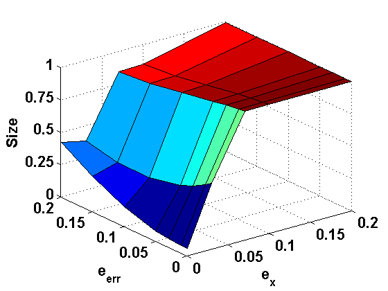
(a) $n=30$, $\tau=\gamma=0$

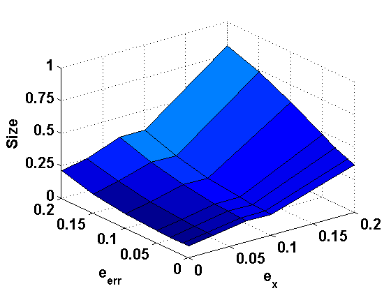
(b) $n=30$, $\tau=\gamma=0.5$

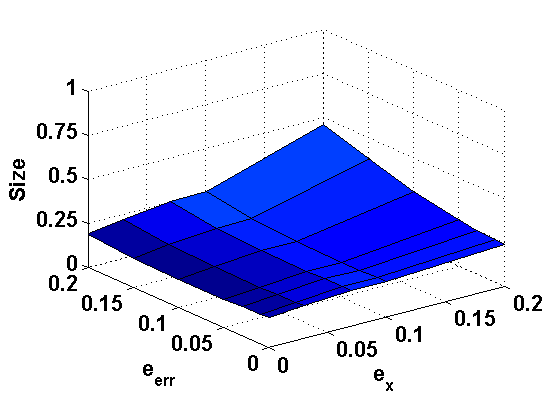
(c) $n=30$, $\tau=\gamma=1$

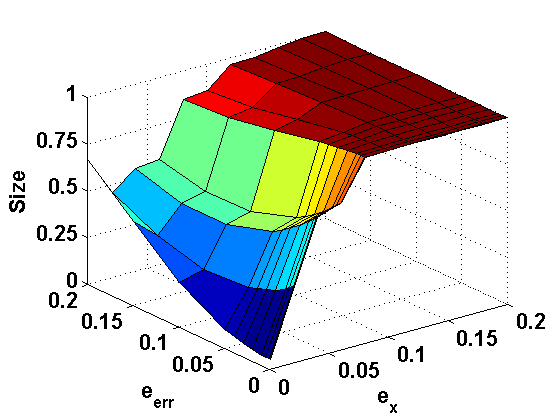
(d) $n=50$, $\tau=\gamma=0$

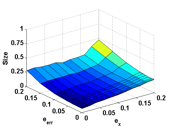
(e) $n=50$, $\tau=\gamma=0.5$

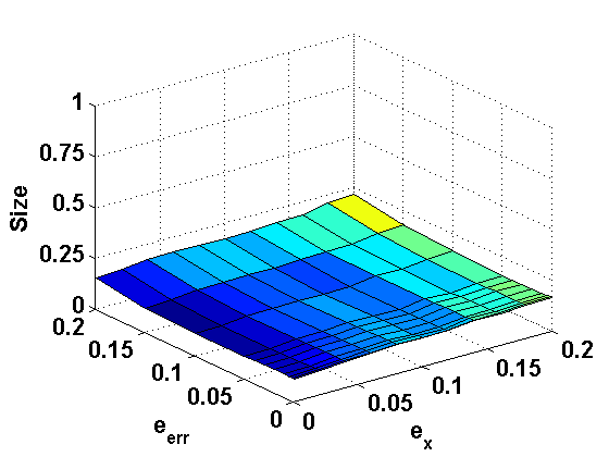
(f) $n=50$, $\tau=\gamma=1$

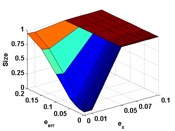
(g) $n=100$, $\tau=\gamma=0$

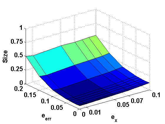
(h) $n=100$, $\tau=\gamma=0.5$

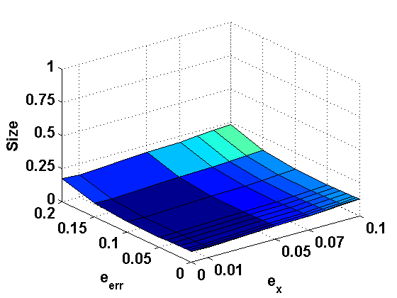
(i) $n=100$, $\tau=\gamma=1$

Figure 1: Empirical size of the DPD based test of ${\boldsymbol{\beta}}$ with unknown $\sigma$ for different sample size $n$ and different $\tau=\gamma$

5 Empirical Illustrations

We now illustrate the claimed robustness of the DPD based tests under an LRM with $\boldsymbol{x}_{i}=(1,z_{i})^{T}$, $z_{i}$ being fixed observation from $N(10,5)$ distribution, and $\boldsymbol{\beta}=(\beta_{1},\beta_{2})^{T}$ for testing the composite null hypothesis $H_{0}:\boldsymbol{\beta}=(3,2)^{T}$ assuming $\sigma$ unknown. We replicate the simulation study of Ghosh and Basu (2018) which studied the robustness of simple null assuming $\sigma$ known. We compute the empirical sizes and powers at the contiguous alternative $H_{1n}:\boldsymbol{\beta}=(3,2)^{T}+\Delta_{n}$, being $\Delta_{n}=\frac{1}{\sqrt{2n}}$, based on 1000 (independent) LRM samples of sizes $n=30,50$ and $100$. In each sample, the errors are generated independently from $(1-e_{err})N(0,3)+e_{err}N(10,3)$ distribution yielding $100e_{err}\%$ outliers in responses with true $\sigma=\sqrt{3}$. We also simultaneously study the effect of leverage points; randomly $100e_{x}\%$ of $z_{i}$s are replaced by observations from $N(16,5)$ distribution or by $\left[{{x}_{i}}(\frac{2-{{\Delta}}}{2})^{2}-{{\Delta}}_{n}\right]$ respectively for size and power calculations. These empirical sizes and powers are presented in Figures 1 and 2 respectively for $\tau=\gamma=0$ (equivalent to LRT), $0.5$ and $1$.

Clearly the LRT ($\tau=\gamma=0$) is highly unstable with respect to both its size and power even for a fairly small contamination in either response or in design space. However, the DPD based tests with larger values of $\tau=\gamma$ are extremely robust against any kind of contamination in the data; their stability in both size and power increases as $\alpha$ increases. This further justifies all theoretical robustness results derived here.

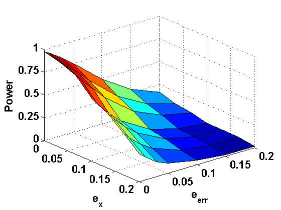
(a) $n=30$, $\tau=\gamma=0$

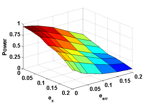
(b) $n=30$, $\tau=\gamma=0.5$

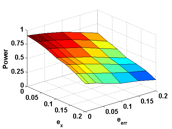
(c) $n=30$, $\tau=\gamma=1$

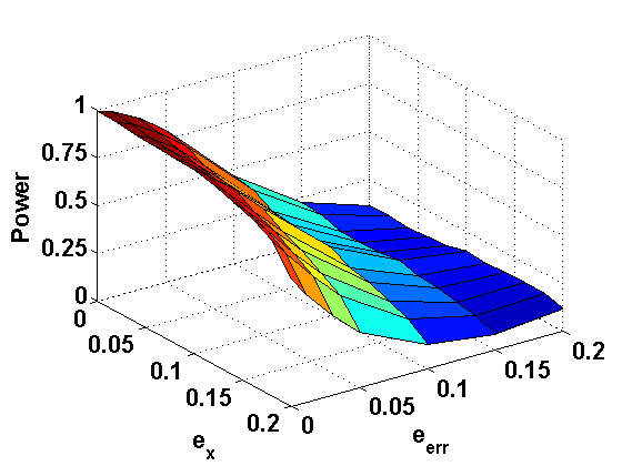
(d) $n=50$, $\tau=\gamma=0$

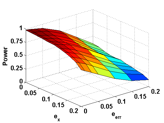
(e) $n=50$, $\tau=\gamma=0.5$

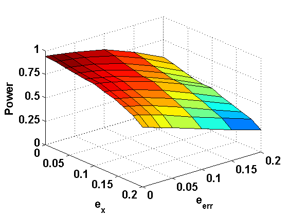
(f) $n=50$, $\tau=\gamma=1$

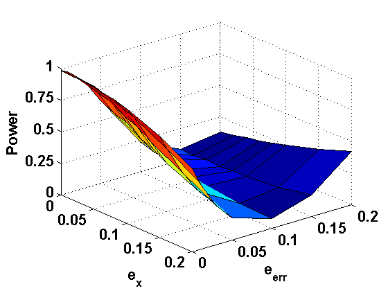
(g) $n=100$, $\tau=\gamma=0$

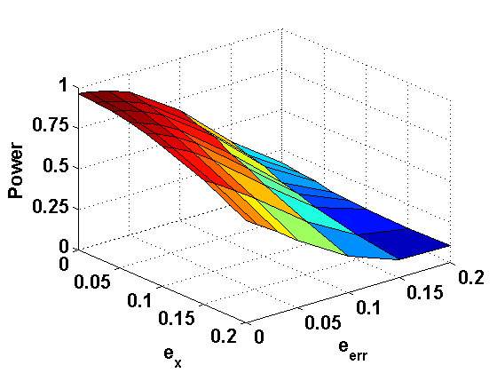
(h) $n=100$, $\tau=\gamma=0.5$

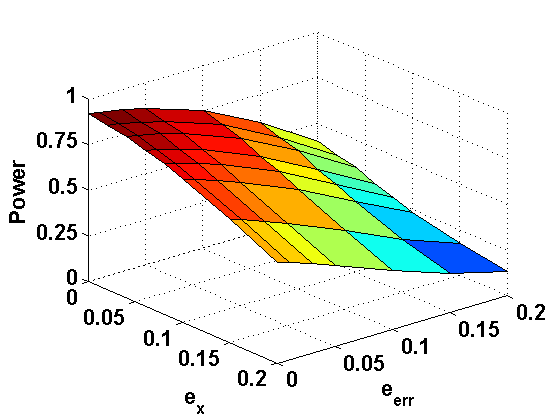
(i) $n=100$, $\tau=\gamma=1$

Figure 2: Empirical power of the DPD based test of ${\boldsymbol{\beta}}$ with unknown $\sigma$ for different sample power $n$ and different $\tau=\gamma$

6 Discussions

This paper fills up the gaps of power and level robustness in the literature of DPD based robust tests for composite hypotheses. The PIF and LIF are derived for general INH set-up and applied to the fixed-carrier linear regression model. Further extension of the concept of PIF and LIF for two or multi-sample problems under the INH set-up will be an interesting future work.

Appendix A Notations

$\boldsymbol{0}_{p}$ denotes $p$-vector of zeros; $\boldsymbol{O}_{p\times q}$ denotes null matrix of order $p\times q$ and $\boldsymbol{I}_{p}$ denotes identity matrix of order $p$.

$${\boldsymbol{u}_{i}}(y;{\boldsymbol{\theta}}) = \nabla\ln f_{i}(y;{\boldsymbol{\theta}})~{}~{}\mbox{ with $\nabla$ representing gradient with respect to $\boldsymbol{\theta}$}$$

$$H_{n}({\boldsymbol{\theta}}) = \frac{1}{n}\sum_{i=1}^{n}V_{i}(Y_{i};{\boldsymbol{\theta}}),\mbox{ with }V_{i}(y;{\boldsymbol{\theta}})=\int f_{i}(y;{\boldsymbol{\theta}})^{1+\tau}dy-\left(1+\frac{1}{\tau}\right)f_{i}(Y_{i};{\boldsymbol{\theta}})^{\tau}$$

$$\boldsymbol{\xi}_{i}({\boldsymbol{\theta}}^{g}) = \int{\boldsymbol{u}_{i}}(y;{\boldsymbol{\theta}}^{g})f_{i}(y;{\boldsymbol{\theta}}^{g})^{\tau}g_{i}(y)dy.$$

$$\boldsymbol{\Psi}_{n}^{\tau}({\boldsymbol{\theta}}^{g}) = \frac{1}{n}\sum_{i=1}^{n}\left[\int{\boldsymbol{u}_{i}}(y;{\boldsymbol{\theta}}^{g}){\boldsymbol{u}_{i}}^{T}(y;{\boldsymbol{\theta}}^{g})f_{i}^{1+\tau}(y;{\boldsymbol{\theta}}^{g})dy\right.$$

$$- \left.\int\{\mathbf{\nabla}{\boldsymbol{u}_{i}}(y;{\boldsymbol{\theta}}^{g})+\tau{\boldsymbol{u}_{i}}(y;{\boldsymbol{\theta}}^{g}){\boldsymbol{u}_{i}}^{T}(y;{\boldsymbol{\theta}}^{g})\}\{g_{i}(y)-f_{i}(y;{\boldsymbol{\theta}}^{g})\}f_{i}(y;{\boldsymbol{\theta}}^{g})^{\tau}dy\right],$$

$$\boldsymbol{\Omega}_{n}^{\tau}({\boldsymbol{\theta}}^{g}) = \frac{1}{n}\sum_{i=1}^{n}\left[\int{\boldsymbol{u}_{i}}(y;{\boldsymbol{\theta}}^{g}){\boldsymbol{u}_{i}}^{T}(y;{\boldsymbol{\theta}}^{g})f_{i}(y;{\boldsymbol{\theta}}^{g})^{2\tau}g_{i}(y)dy-\boldsymbol{\xi}_{i}({\boldsymbol{\theta}}^{g})\boldsymbol{\xi}_{i}^{T}({\boldsymbol{\theta}}^{g})\right],$$

$$\boldsymbol{P}_{n}^{\tau}({\boldsymbol{\theta}}) = \left[\frac{\nabla^{2}H_{n}({\boldsymbol{\theta}})}{(1+\tau)}\right]^{-1}\left[\boldsymbol{I}_{p}-\boldsymbol{\Upsilon}({\boldsymbol{\theta}})\boldsymbol{\Upsilon}^{\ast}({\boldsymbol{\theta}})^{-1}\boldsymbol{\Upsilon}({\boldsymbol{\theta}})^{T}[\nabla^{2}H_{n}({\boldsymbol{\theta}})]^{-1}\right].$$

with $$\boldsymbol{\Upsilon}({\boldsymbol{\theta}})=\frac{\partial\boldsymbol{\upsilon}({\boldsymbol{\theta}})}{\partial{\boldsymbol{\theta}}}\mbox{ and }\boldsymbol{\Upsilon}^{\ast}({\boldsymbol{\theta}})=\left[\boldsymbol{\Upsilon}({\boldsymbol{\theta}})^{T}[\nabla^{2}H_{n}({\boldsymbol{\theta}})]^{-1}\boldsymbol{\Upsilon}({\boldsymbol{\theta}})\right]$$

$$\boldsymbol{A}_{n}^{\gamma}({\boldsymbol{\theta}}) = \frac{1}{n}\sum_{i=1}^{n}\boldsymbol{A}_{\gamma}^{(i)}({\boldsymbol{\theta}})~{}~{}\mbox{ with }~{}~{}\boldsymbol{A}_{\gamma}^{(i)}({\boldsymbol{\theta}}_{0})=\nabla^{2}d_{\gamma}(f_{i}(.;{\boldsymbol{\theta}}),f_{i}(.;{\boldsymbol{\theta}}_{0}))\big{|}_{{\boldsymbol{\theta}}={\boldsymbol{\theta}}_{0}}.$$

$$\boldsymbol{M}_{j,\gamma}^{(i)}({\boldsymbol{\theta}}_{1},{\boldsymbol{\theta}}_{2}) = \frac{\partial}{\partial\boldsymbol{\theta}_{j}}d_{\gamma}(f_{i}(.;{\boldsymbol{\theta}}_{1}),f_{i}(.;{\boldsymbol{\theta}}_{2})),~{}~{}j=1,2;~{}i=1,\ldots,n.$$

$$\boldsymbol{A}_{j,k,\gamma}^{(i)}({\boldsymbol{\theta}}_{1},{\boldsymbol{\theta}}_{2}) = \frac{\partial^{2}}{\partial\boldsymbol{\theta}_{j}\boldsymbol{\theta}_{k}}d_{\gamma}(f_{i}(.;{\boldsymbol{\theta}}_{1}),f_{i}(.;{\boldsymbol{\theta}}_{2})),~{}~{}j,k=1,2;~{}i=1,\ldots,n.$$

References

• Basu etΒ al. (1998) Basu, A., Harris, I.Β R., Hjort, N.Β L., and Jones M.Β C. (1998). Robust and efficient estimation by minimising a density power divergence. BiometrikaΒ 85, 549–559.
• Basu etΒ al. (2013) Basu, A., Mandal, A., Martin, N., and Pardo, L.Β (2013). Testing statistical hypotheses based on the density power divergence. Ann. Inst. Statist. Math.Β 65, 319–348.
• Basu etΒ al. (2011) Basu, A., Shioya, H. and Park, C. (2011). Statistical Inference: The Minimum Distance Approach. Chapman & Hall/CRC. Boca Raton, Florida.
• Ghosh (2017a) Ghosh, A.Β (2017a). Divergence based Robust Estimation of Tail Index with Exponential Regression Model. Statist Method Appl.Β 26(2), 181–213.
• Ghosh (2017b) Ghosh, A. (2017b). Robust Inference under the Beta Regression Model with Application to Health Care Studies. Statistical Methods in Medical Research, doi:10.1177/0962280217738142.
• Ghosh and Basu (2013) Ghosh, A. and Basu, A.Β (2013). Robust Estimation for Independent Non-Homogeneous Observations using Density Power Divergence with Applications to Linear Regression. Electron. J. statist.Β 7, 2420–2456.
• Ghosh and Basu (2015) Ghosh, A. and Basu, A.Β (2015). Robust Estimation for Non-Homogeneous Data and the Selection of the Optimal Tuning Parameter: The DPD Approach. J. App. Statist., 42(9), 2056–2072.
• Ghosh and Basu (2016) Ghosh, A. and Basu, A.Β (2016). Robust Estimation in Generalised Linear Models : The Density Power Divergence Approach. TEST, 25(2), 269–290.
• Ghosh and Basu (2018) Ghosh, A. and Basu, A.Β (2018). Robust Bounded Influence Tests for Independent Non-Homogeneous Observations. Statistica Sinica, 28(3), 1133–1155.
• Hampel etΒ al. (1986) Hampel, F.Β R., E.Β Ronchetti, P.Β J. Rousseeuw, and W.Β Stahel (1986). Robust Statistics: The Approach Based on Influence Functions. John Wiley & Sons.
• Heritier and Ronchetti (1994) Heritier, S. and Ronchetti, E. (1994). Robust bounded-influence tests in general parametric models. J. Amer. Statist. Assoc.Β 89, 897–904.
• Huber-Carol (1970) Huber-Carol, C. (1970). Etude asymptotique de tests robustes. Ph.D. thesis, ETH, Zurich.
• Kotz etΒ al. (1967) Kotz, S., Johnson, N.Β L., and Boyd, D.Β W. (1967). Series representations of distributions of quadratic forms in normal variables.Β I.Β Non-central case. Ann. Math. Statist.Β 38, 838–848.
• Lehmann (1983) Lehmann, E.Β L. (1983). Theory of Point Estimation. John Wiley & Sons.
• Toma and Broniatowski (2010) Toma, A. and M.Β Broniatowski (2010). Dual divergence estimators and tests: robustness results. J. Mult. Anal.Β 102, 20–36.