Observational assessment of the viability of de Sitter Gödel de Sitter phase transition

Abstract

de Sitter–Gödel–de Sitter phase transition(dGd) is a possible geometrical phase transition in the very early universe. It induces fluctuations with possibly observable traces on matter and radiation fields. Here we present a simulation based on dGd to investigate possible perturbations which could be along with the standard inflationary fluctuations in the cosmic microwave background (CMB) and distribution of the large-scale structure. The power spectrum of perturbations is characterized by a parameter pair, labeled here as ($p_{1},p_{2}$). With Planck observations we find $p_{1}=0.008^{+0.003}_{-0.008}$ and $p_{2}=0.002^{+0.001}_{-0.002}$ consistent with pure inflationary power spectrum and no hint for the dGd transition. Also, it is estimated future large-scale surveys such as Euclid and SKA can further tighten the constraints up to an order of magnitude and probe the physics of the early universe with much higher precision.

I Introduction

Rotation is a universal phenomenon observed on a wide variety of scales in high-energy physics and astrophysics. Also, the origin of rotation is one of the most intriguing issues of cosmology. Thanks to many redshift large area surveys(Davis et al., 1982; Colless et al., 2001; York et al., 2000), our knowledge about structure formation have increased, and now we know that most structures in cosmology are in a rotating state.

Any theory of structure formation should explain the presence of rotation and clarify its origin(Korotky et al., 2020). The later growth of structures in the nonlinear regime could cause structures to spin without any initial angular momentum. In the linear regime, however, a mechanism is required to initiate the rotation. Structures on scales of several Mega Parsecs like filaments, walls and voids provide an environment to test theories of linear and quasi-linear regimes(Bernardeau, 1996; Conroy et al., 2005; Croton and Farrar, 2008; Sousbie et al., 2007; Bond et al., 2010; Choi et al., 2010). Surprisingly a recent observational effort gives some evidence for the spin of cosmic filaments(Wang et al., 2021).

Theoretically, we know rotation is usually associated with vorticity. Therefore it can not be generated in a perfect fluid in perturbation theory and inflation scenarios. In particular, as the universe expands, any primordial vorticity will be redshifted away and would not be affected by the density perturbation growth(Lu et al., 2009). Tidal Torque Theory (TTT) is the traditional formalism for analyzing the initial spin in the framework of the standard model of cosmology(Hoyle, 1951; Peebles, 1969; White, 1984). Most literature follow TTT to explain the origin of rotation in linear and quasi-linear regimes, but the main issue is still an open question(Porciani et al., 2002; van de Weygaert et al., 2016; Pichon et al., 2014; Kim et al., 2022).

Another suggestion for the origin of rotation backs to G. Gamow(Gamow, 1946). It is possible to consider the universe to be born with spin. Some cosmological models assume that the primordial universe not only expands but also rotates(Godel, 1949; Barrow et al., 1985; Sivaram and Arun, 2012). But it has to be noted that due to the observational assessment, a global rotation is less than $10^{-13}rad\ y^{-1}$(Li, 1998), and thus the idea of global rotation is not acceptable.

On the other hand, the early universe is a unique laboratory to test theories of high energy physics which are inaccessible to earth-bound experiments. Among these theories are possible cosmological phase transitions at different epochs depending on the energy scales involved (e.g. see (Gangui, 2001; Hindmarsh and Kibble, 1995; Vilenkin and Shellard, 2000)). If these transitions leave observable cosmological imprints, e.g. if they generate fluctuations on the CMB radiation and matter fields, they would have the chance to be tested against data while their parameter $\beta$ would be constrained (see Ref. (Ade et al., 2014) for constraints on the cosmic string tension from Planck CMB observations).

Among plausible phase transitions in the early universe is de Sitter–Gödel–de Sitter (dGd) phase transition which is a quantum phase transition of spacetime (Khodabakhshi and Shojai, 2015). The dGd scenario assumes a scalar field in a de Sitter background would experience a phase transition to a rotating Gödel geometry and slowly rolls back to the de Sitter phase.

The dGd transition could be a possible source of initial rotation for large structures. This is particularly of interest since as mentioned before simple inflationary theories do not seed vector modes and therefore no initial spin is expected for the largest scale structure in pure inflationary cosmologies. As well, although TTT is the standard method, it is not the ultimate answer to the origin of rotation and is dependent on lots of numerical simulations and methods.

Quantum field theory calculations at finite temperature show that dGd second-order phase transition has a chance to occur at high temperatures. Then the transition probability depends on the rotation parameter of the Gödel phase ($\alpha$), increasing as $\alpha$ decreases. This rotation will be induced on the trajectories of test particles. Simulations show local congruence of particles has nonzero induced rotation while the average global rotation is almost zero(Khodabakhshi and Shojai, 2015).

Furthermore, it was shown that Casimir force in the dGd transition induces inhomogeneities in the matter and radiation fields, possibly observable in the CMB radiation or large-scale structure data (Khodabakhshi and Shojai, 2017). The predictions of the dGd transition can therefore be directly tested against the existing data. Observational assessment of the viability of this theory and estimating the model parameters are the main goals of this paper.

This paper is structured as follows: We explain and review the dGd model in sections 2 and 3. In Section 4, we simulate primordial seeds of inhomogeneities produced by the dGd transition and assess the trace of primordial seeds (alongside inflationary perturbations) on CMB anisotropies. Also, we explore how future large-scale surveys improve the bounds of model parameters. Finally, in Section 5, we discuss our conclusion.

II Review of dGd phase transition (Global features)

The extremely high temperature of the early universe allows for a scenario where a quantum mechanical phase transition could change the geometry of spacetime, which could occur due to a phase transition in the potential of a scalar field. Since

$$p_{\phi}=\frac{1}{2}\dot{\phi}^{2}-V(\phi)-\frac{1}{2}\left|\vec{\nabla}\phi\right|^{2}$$ (1)

$$\rho_{\phi}=\frac{1}{2}\dot{\phi}^{2}+V(\phi)+\frac{1}{2}\left|\vec{\nabla}\phi\right|^{2},$$ (2)

a spatially constant and time independent scalar field $\phi$, ($\dot{\phi}=0$ and $\vec{\nabla}\phi=0$) , acts as a perfect fluid with energy density and pressure given by $p_{\phi}=-\rho_{\phi}$ which is the equation of state of cosmological constant. Therefore we can consider $V(\phi)$ as an effective cosmological constant(Hobson et al., 2006). Thus, the effective potential in curved spacetime would be an apt tool to continue. The action of a scalar field in a curved spacetime $g_{\mu\nu}$ is (Mukhanov and Winitzki, 2007)

$$S[\phi,g_{\mu\nu}]=\int d^{4}x\sqrt{-g}\left(\frac{1}{2}\partial_{\mu}\phi\partial^{\mu}\phi-V(\phi)\right)\ .$$ (3)

Straightforwardly we can calculate the one-loop effective potential from

$$V^{(1)}_{\textrm{eff}}=-\frac{\Gamma^{(1)}}{\cal{V}}$$ (4)

where $\cal{V}$ is the spatial volume. $\Gamma^{(1)}=-\frac{i}{2}\ln(\mu^{-2}\det G)$ is the one-loop effective action, $G=\square+V^{\prime\prime}$ and $\mu$ is introduced for dimensional considerations. Also $\square$ operator is defined as $\square\phi=|g|^{-1/2}\partial_{\mu}(|g|^{1/2}g^{\mu\nu}\partial_{\nu}\phi)$ for a surrounding metric $g_{\mu\nu}$.

Now we briefly review the model. The dGd requires a situation where the background geometry of the universe would change from de Sitter to Gödel for some small enough time and then quickly to de Sitter through a thermal phase transition of the scalar field.

The dGd phase transition is supposed to occur just after inflation. The scalar field could be the inflaton field. Since we are working at a finite temperature regime and the wick rotation in curved space can only be adopted for stationary spacetimes, the model is restricted to the static chart of de Sitter, so that wick rotation could be applied. The static patch of de Sitter spacetime is described in $(t,\chi,\theta,\xi)$ coordinates by (Fursaev and Miele, 1994)

$$\rm ds^{2}=\cos^{2}\chi d\tau^{2}+a^{2}(d\chi^{2}+\sin^{2}\chi d\theta^{2}+\sin^{2}\chi\sin^{2}\theta d\xi^{2})$$ (5)

where $a^{2}=2/\Lambda$ is the spatial scale and $-\infty<t=-i\tau<+\infty$, $-\pi<\chi<\pi$, $0<\theta$, $\xi<\pi$. The range of periodic parameter $\tau$ is from $0$ to $\beta$. We assume the classical potential for $\phi$ is

$$V=\frac{1}{2}\sigma^{2}\phi^{2}+\frac{1}{24}\lambda\phi^{4}$$ (6)

With $\sigma$ and $\lambda$ to be an arbitrary mass scale and a dimensionless coupling constant, respectively. Using the zeta-function $(\zeta)$ regularization method, the corresponding effective potential to (6) is

$$V_{\textrm{eff}}(\phi,\beta)=V(\phi)-\\ \frac{1}{2\beta\cal V}\left[\zeta^{\prime}(0,\beta)+\log(\mu^{2}a^{2})\zeta(0,\beta)+\log(V^{\prime\prime}(\phi)\mu^{-2})\right]$$ (7)

where $\beta=(k_{B}T)^{-1}$ (Elizalde et al., 1994). Following calculations of (Khodabakhshi and Shojai, 2015) we find the effective potential in de Sitter background

$$\frac{\lambda}{2\sigma^{4}}V_{\textrm{eff}}=\frac{\lambda}{2\sigma^{4}}V_{0}+\frac{1}{2}x^{2}+\frac{1}{12}x^{4}\\ -\gamma T\bigg{\{}0.62\Delta-0.22\Delta^{2}+0.075T+\frac{T^{3}}{120}\\ +\frac{1}{T}\left(-0.07+2.7\Delta^{2}-0.15\Delta\right)\\ +\left(0.22-\frac{2.7}{T}\right)\left(\frac{51-60T^{2}-8T^{4}}{240}-\frac{2T^{2}-3}{2}\Delta+\Delta^{2}\right)\\ +\log[\mathfrak{a}(1+x^{2})]\bigg{\}}\$$ (8)

where $\mathfrak{a}=a^{2}\sigma^{2}$, $\gamma=\frac{3\lambda}{32\pi^{2}\mathfrak{a}^{2}}$, $x=\sqrt{\frac{\lambda}{2}}\frac{\phi}{\sigma}$, $\Delta=\frac{9}{4}-\mathfrak{a}(1+x^{2})$, and $T=\frac{\beta_{H}}{\beta}=\frac{2\pi a}{\beta}$.

This potential has extremum at

$$x=0$$ (9)

and at the roots of the equation

$$1+\frac{1}{3}x^{3}-\gamma T\bigg{\{}-1.24\mathfrak{a}+0.44\Delta-\frac{10.8}{T}\Delta+\frac{0.3\mathfrak{a}}{T}\\ \mathfrak{a}\left(0.22-\frac{2.7}{T}\right)(2T^{2}-3-4\Delta)+\frac{2}{1+x^{2}}\bigg{\}}\ .$$ (10)

It is clear that if this equation has no real root, the potential is a harmonic-type. Otherwise, it has a Mexican hat shape. There are some regions of parameters $\mathfrak{a}$, $\gamma$ and temperature $T$ which allow a Mexican hat shape for Eq. 8. Typical shape of the effective potential is plotted in figure 1 for some different values of temperature, $\mathfrak{a}=2$ and $\gamma=10$.

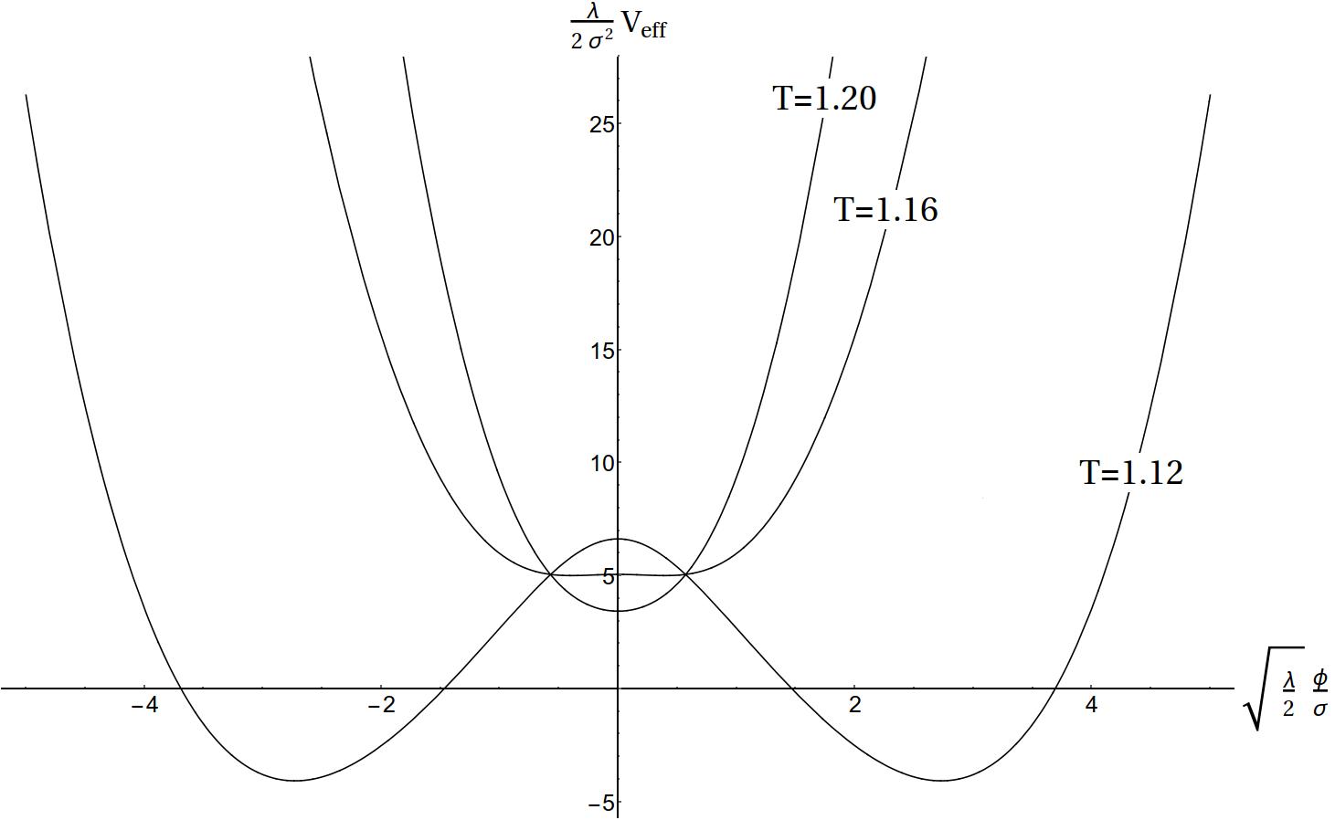
Figure 1: The one-loop potential for different values of temperature, $\mathfrak{a}=2$ and $\gamma=10$ taken from (Khodabakhshi and Shojai, 2015).

Therefore, during the universe cooling, we can find a critical temperature in which the scalar field experiences a phase transition so that the effective potential is negative. At this temperature and when the depth of the Mexican hat is equal to $-\Lambda=\rho_{\textrm{dust}}/2$, we assume the universe has Gödel geometry. Then we can evaluate the one-loop potential with Gödel metric, which is an exact dust solution of Einstein field equations via a negative cosmological constant, described in Cartesian coordinates $(t,x,y,z)$ by (Godel, 1949)

$$\rm ds^{2}=(dt+\exp^{\sqrt{2}\alpha x/2}dy)^{2}-dx^{2}-\frac{1}{2}\exp^{\sqrt{2}\alpha x}dy^{2}-dz^{2}$$ (11)

where $\alpha$ gives the angular momentum four-vector $\alpha^{\beta}=(0,0,0,\alpha)$ of intrinsic rotation. Following calculations of (Huang, 1991), we can calculate the effective potential in Gödel spacetime

$$V_{\textrm{eff}}=\bar{V}_{0}+\frac{\sigma^{4}}{16\pi^{3/2}}\left(\frac{\alpha^{2}}{8\sigma^{2}}+\frac{M^{2}}{\sigma^{2}}\right)^{3/2}\times\\ \bigg{\{}\frac{2\sqrt{\pi}}{3}-\sum_{n,\ell}^{{}^{\prime}}\left(2Z^{\nu-3/2}_{1}K_{3/2-\nu}(2Z_{1})\right.\\ \left.-Z^{\nu-3/2}_{2}K_{3/2-\nu}(2Z_{2})\right)\bigg{\}}$$ (12)

where $\bar{V}_{0}$ is a constant and $M^{2}=\sigma^{2}+\frac{1}{2}\lambda\phi^{2}$. Prime on the summation means the term $n=\ell=0$ is neglected. $K$ is the modified Bessel function, and $Z$ is the Epstein zeta function

$$Z_{1}=\pi\sqrt{\left(\frac{\alpha^{2}}{8}+M^{2}\right)\left(\frac{\ell^{2}}{4\pi^{2}\bar{T}^{2}\sigma^{2}}+\frac{8n^{2}}{\alpha^{2}}\right)}$$ (13)

$$Z_{2}=\pi\sqrt{\left(\frac{\alpha^{2}}{8}+M^{2}\right)\left(\frac{\ell^{2}}{4\pi^{2}\bar{T}^{2}\sigma^{2}}+\frac{2n^{2}}{\alpha^{2}}\right)}$$ (14)

where $\bar{T}^{-1}=\beta\sigma$. In $\bar{\alpha}=8\sigma^{2}/\alpha^{2}\gg 1$ and $\bar{T}\gg 1$ limits, the renormalized effective potential with dimensionless quantities is

$$\frac{\lambda}{2\sigma^{4}}V_{\textrm{eff}}=\frac{\lambda}{2\sigma^{4}}\bar{V}_{0}-\bar{\gamma}\bar{T}\left(1+\bar{\alpha}(1+x^{2})\right)^{1/4}\\ \times\exp\left(-\pi\sqrt{1+\bar{\alpha}(1+x^{2})}\right)$$ (15)

where $\bar{\gamma}=\frac{\lambda\alpha^{2}}{16\pi^{2}\sqrt{2}\sigma^{2}}$. The one-loop effective potential shape with these limits, is presented in figure 2.

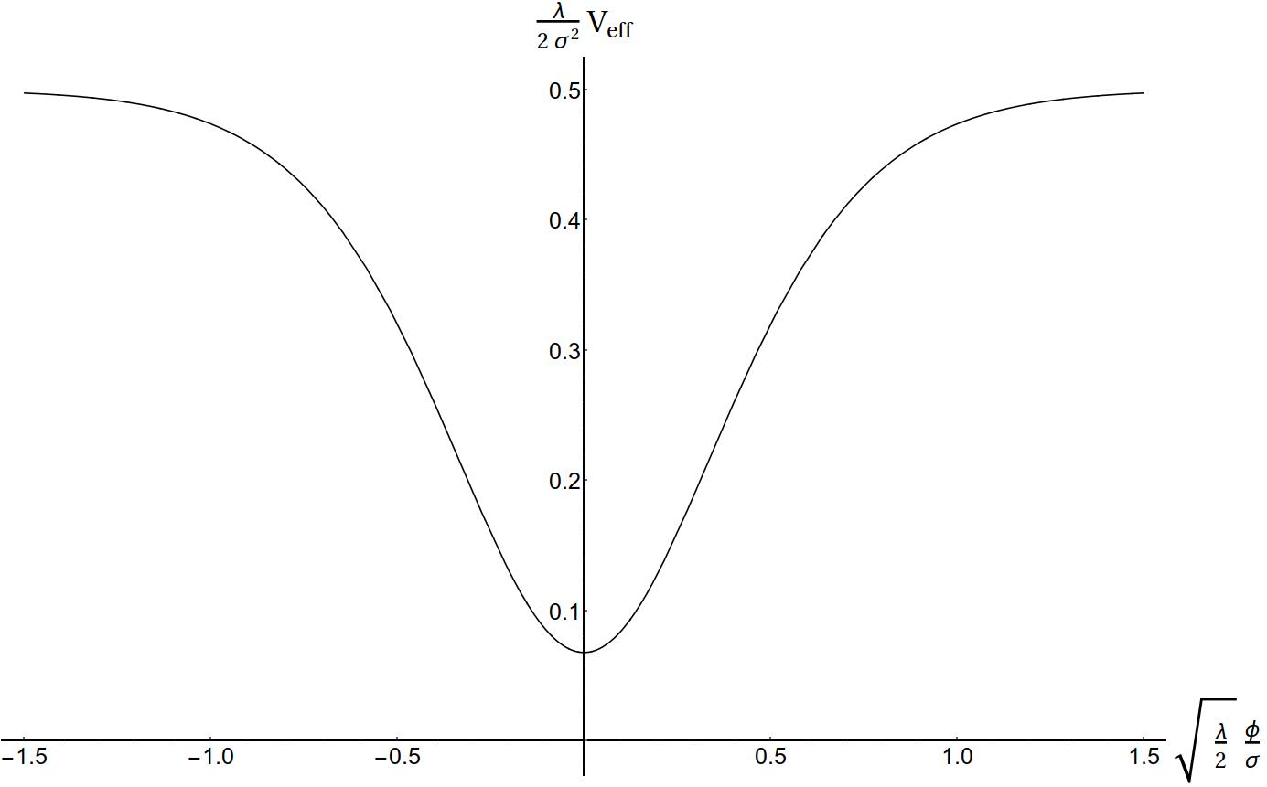
Figure 2: one-loop effective potential in Gödel spacetime with $\bar{\alpha}=3$, $\bar{\gamma}\bar{T}=10$, and $\frac{\lambda V_{0}}{2\sigma^{2}}=0.5$, taken from (Khodabakhshi and Shojai, 2015) .

Here $\alpha$ is a nonzero real constant which shows the rotation rate of dust around the $y$-axis. The Gödel phase can naturally initiate the rotation since it is a rotating spacetime. In this phase, $V_{\textrm{eff}}=-\rho_{\textrm{dust}}/2$ and has the role of a negative cosmological constant. Finally, the shape of the effective potential in the Gödel background allows for the rolling of the scalar field such that the universe goes back to the de Sitter phase with a positive sign of effective potential.

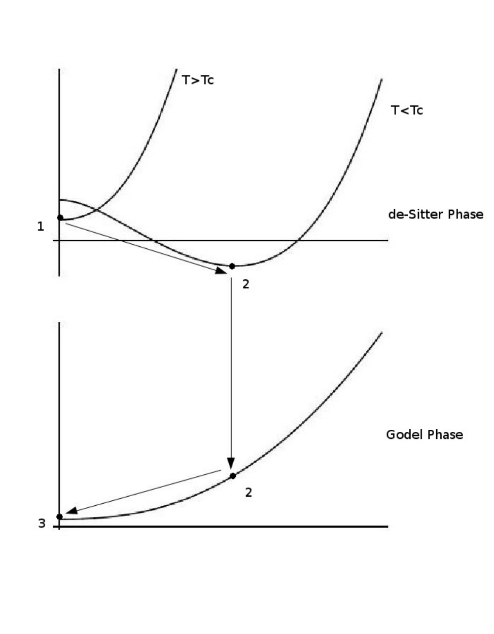
Figure 3: Typical scenario of the initial de Sitter, Gödel and final de Sitter phases, taken from (Khodabakhshi and Shojai, 2015).

Figure (3) shows a typical scenario to understand the whole story in three steps. First, $V_{\textrm{eff}}$ is much larger than the dust density $V_{\textrm{eff}}\gg\rho_{\textrm{dust}}$ and is positive so it can act like a positive cosmological constant. After enough cooling due to the expansion, the universe can reach a critical temperature $\beta_{c}$ where $\left.\frac{d^{2}V_{\textrm{eff}}}{d\phi^{2}}\right|_{\phi=0}=0$. Below $\beta_{c}$, the scalar field can experience a phase transition to the Mexican hat potential with a negative cosmological constant which describes a Gödel phase. Then the scalar field can roll down the potential until $\phi=0$. After $\tilde{t}\simeq\frac{\phi}{\dot{\phi}}\simeq\frac{\sigma}{\sqrt{\lambda\Lambda}}$ (which is the time duration of dGd phase transition), the universe would go back to a de Sitter phase again.

The impact of dGd on the equations of motion of a test particle is explored in (Khodabakhshi and Shojai, 2015). As intuitively expected, a particle that enters the first de Sitter phase with a non-rotating trajectory exits to the final de Sitter phase while it is rotating. In other words, this phase transition induces rotation in the motion of test particles. The value of the induced rotation depends on the particle position in the de Sitter space, its distance from the symmetry axis of Gödel, and the initial velocity, and it is of order $\sqrt{\Lambda}$. This mechanism also works for the congruence of particles. Simulations show a local congruence of particles would obtain nonzero local induced rotation. Also if we divide the universe into cells and simulate the dGd transition based on the quantum tunneling probability and the randomness of the symmetry axis of Gödel space direction, we will find the average global induced rotation is nearly zero, as expected. See Figures 5 and 7 of (Khodabakhshi and Shojai, 2015).

III Local features of dGd

III.1 Israel junction condition

Casimir force comes from zero-point oscillations of quantized field between two boundaries (Bordag et al., 2009). We can assume the universe is built from a 3D lattice with $n^{3}$ cubic cells with side $d$ as Figure 4. Each cell could experience the dGd phase transition. Thus, if the rotation direction of neighboring rotating cells is different (Figure 4), then the Israel density at the boundaries of each of them, leads to a Casimir force. Isreal density is nothing but the jump at the intrinsic curvature (Poisson, Eric, 2002)

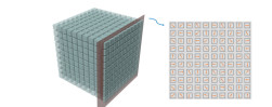
Figure 4: universe as a 3D lattice (left). The cells experience rotations around random axes (right).(taken from (Khodabakhshi and Shojai, 2017))

$$S_{ab}\propto[K_{ab}]-[K]h_{ab}\ ,$$ (16)

where $[K_{ab}]=K_{ab}^{(2)}-K_{ab}^{(1)}$ and $K_{ab}^{(i)}\equiv n_{(\alpha;\beta)}e^{\alpha\ (i)}_{a}e^{\beta\ (i)}_{b}$ .

In our model, the jump in the intrinsic curvature is a consequence of the random direction of Gödel cells. To have a rare estimation of this density, we use the Gödel metric in cylindrical coordinates,

$$d\rm s^{2}=\frac{2}{\alpha^{2}}\bigl{[}dt^{2}-dr^{2}-dz^{2}+(\sinh^{4}r-\sinh^{2}r)d\phi^{2}\\ \rm+2\sqrt{2}\sinh^{2}rd\phi dt\bigr{]}\ .$$ (17)

Without loss of generality, we assume a hypersurface between two cells is determined by the normal $n=(0,\sin\phi,\cos\phi,0)$. Thus, at one side the extrinsic curvature $K^{(1)}_{ab}$ is

$$\begin{pmatrix}0&\sqrt{2}\cos{\phi}\operatorname{csch}{r}\operatorname{sech}{r}&-\sqrt{2}\sin{\phi}\cosh{r}\sinh{r}\\ \sqrt{2}\cos{\phi}\operatorname{csch}{r}\operatorname{sech}{r}&0&\dfrac{1}{2}\cos{\phi}-\cos{\phi}\operatorname{csch}{r}\operatorname{sech}{r}\\ -\sqrt{2}\sin{\phi}\cosh{r}\sinh{r}&\dfrac{1}{2}\cos{\phi}-\cos{\phi}\operatorname{csch}{r}\operatorname{sech}{r}&-\dfrac{1}{4}\bigl{(}4-4\sinh{2r}+\sinh{4r}\bigr{)}\sin{\phi}\end{pmatrix}$$ (18)

while on the other side this quantity is the one which is fixed by the rotated local tetrads concerning the previous one. Up to our simple estimation, it would be acceptable and more fanciable if we rotate the deviation of the normal vector, $n_{(\alpha;\beta)}$, rather than the tetrads. Thus, for $n^{\prime}=(0,\cos(\phi),-\sin(\phi),0)$, the $K^{(2)}_{ab}$ is

$$\begin{pmatrix}0&-\sqrt{2}\sin{\phi}\operatorname{csch}{r}\operatorname{sech}{r}&-\sqrt{2}\cos{\phi}\cosh{r}\sinh{r}\\ -\sqrt{2}\sin{\phi}\operatorname{csch}{r}\operatorname{sech}{r}&0&\dfrac{1}{2}\bigl{(}\sin{\phi}\operatorname{csch}{r}\operatorname{sech}{r}+(\operatorname{csch}{r}\operatorname{sech}{r}-1)\sin{\phi}\bigr{)}\\ -\sqrt{2}\cos{\phi}\cosh{r}\sinh{r}&\dfrac{1}{2}\bigl{(}\sin{\phi}\operatorname{csch}{r}\operatorname{sech}{r}+(\operatorname{csch}{r}\operatorname{sech}{r}-1)\sin{\phi}\bigr{)}&-\dfrac{1}{4}\bigl{(}4-4\sinh{2r}+\sinh{4r}\bigr{)}\cos{\phi}\end{pmatrix}$$ (19)

Therefore, the Israel density for this choice is about

$$S_{00}\propto\dfrac{1}{4}\bigl{(}4-4\sinh{2r}+\sinh{4r}\bigr{)}\cos{\phi}\operatorname{csch}^{2}{r}\operatorname{sech}^{2}{r}\\ -\dfrac{1}{4}\bigl{(}4-4\sinh{2r}+\sinh{4r}\bigr{)}\operatorname{csch}^{2}{r}\operatorname{sech}^{2}{r}\sin{\phi}\ .$$ (20)

Although the precise value of this quantity is obtained by calculating the Root mean square over all possible orientations of the neighboring cells, the nonvanishing result of Eq. 20 is enough motivation for the following discussions.

III.2 Casimir effect

As discussed, the nonvanishing expression of the Israel junction condition shows after the dGd phase transition, the distance between local layers of matter can shrink in a direction perpendicular to the random Gödel rotation axis in an inhomogeneous way. This can cause a Casimir effect in the Gödel phase. The Casimir energy of a scalar field in the Gödel background at finite temperature is (Khodabakhshi and Shojai, 2017)

$$\bar{E}_{\textrm{\tiny Casimir}}\left(\bar{d},\bar{\beta}\right) =\bar{E}_{0}\left(\bar{d}\right)+\bar{\Delta}_{\textrm{F.T.}}\left(\bar{d},\bar{\beta}\right)\ .$$ (21)

The zero temperature term $\bar{E}_{0}\left(\bar{d}\right)$, and the finite temperature contribution $\bar{\Delta}_{\textrm{F.T.}}\left(\bar{d},\bar{\beta}\right)$ are respectively given by

$$\bar{E}_{0}(\bar{d})\simeq-\frac{\pi}{24\bar{d}}-\frac{1}{4\sqrt{2}\bar{d}}\exp\left\{-2\left(\frac{1}{2}+\bar{m}^{2}\right)\frac{\bar{d}^{2}}{\pi}\right\},$$ (22)

and

$$\bar{\Delta}_{\textrm{F.T.}}\left(\bar{d},\bar{\beta}\right) =\frac{1}{\bar{\beta}}\ln\bigg{[}\left\{1-\exp\left(-\frac{2\left(\frac{1}{2}+\bar{m}^{2}\right)\bar{d}^{2}}{\pi}\right)\right\}^{\frac{1}{2}}$$

$$\prod_{n_{1},n_{2},n_{3},n_{4}=1}^{\infty} \left\{1-\exp\left(-\bar{\beta}\sqrt{\frac{1}{2}+\bar{m}^{2}+n_{1}^{2}+\frac{\pi^{2}n_{2}^{2}}{\bar{d}^{2}}}\right)\right\}$$

$$\times \left\{1-\exp\left(-\bar{\beta}\sqrt{\frac{1}{2}+\bar{m}^{2}+\frac{\pi^{2}n_{3}^{2}}{\bar{d}^{2}}}\right)\right\}$$

$$\times \left\{1-\exp\left(-2\bar{d}\sqrt{\frac{1}{2}+\bar{m}^{2}+n_{4}^{2}}\right)\right\}^{\frac{1}{2}}\bigg{]}\ .$$ (23)

Here $\bar{\beta}=\beta\alpha$, $\bar{d}=\alpha d$, $\bar{m}=m/\alpha$ and $\bar{E}=E/\alpha$ are dimensionless quantities in natural unites, $\alpha$ is the rotation rate of the Gödel metric (see Eq. 11), $d$ is the distance between plates and $n_{1},n_{2},n_{3},n_{4}$ are introduced in (Khodabakhshi and Shojai, 2017).

Some direct calculation yields the expression for the Casimir force. The general behavior is plotted in Figure 5.

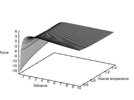
Figure 5: Normalized Casimir force, $\bar{m}=1$(taken from (Khodabakhshi and Shojai, 2017)).

Here we only keep the major contribution to the force given by $n_{1}=n_{2}=n_{3}=n_{4}=1$. The $\bar{d}$-dependence of the Casimir force would then be

$$\mathit{F}_{\textrm{\tiny{Casimir}}}\simeq\mathcal{O}(\frac{1}{\bar{\beta}^{2}\bar{d}^{1/2}})+\mathcal{O}(\frac{\bar{d}^{1/2}}{\bar{\beta}^{2}})+\mathcal{O}(\frac{1}{\bar{\beta}})+\mathcal{O}(\frac{1}{\bar{\beta}\bar{d}^{2}}),$$ (24)

or in terms of $\alpha$:

$$\mathit{F}_{\textrm{\tiny{Casimir}}}\simeq\alpha^{2}\left\{\mathcal{O}(\alpha^{-5/2})+\mathcal{O}(\alpha^{-3/2})+\mathcal{O}(\alpha^{-1})+\mathcal{O}(\alpha^{-3})\right\}\ .$$ (25)

Asymptotically, in the limit of small rotations, we get

$$\mathit{F}_{\textrm{\tiny{Casimir}}}\simeq\frac{1}{\bar{\beta}\bar{d}^{2}}\ .$$ (26)

The Casimir force is sensitive to the rotation angle of the Gödel spacetime. We demonstrated that for two parallel plates with a separation comparable to the rotation of Gödel spacetime ($\alpha$), the force becomes repulsive and then approaches zero. This effect, when considered collectively due to many layers, could induce inhomogeneities that are potentially observable. In the next section, we investigate the observable consequences of dGd transition produced by local Casimir forces.

It may be asked that despite the existence of closed time-like curves (CTCs) and causality violation properties of Gödel spacetime, why such a metric is chosen. Actually, to design a phase transition model to produce rotation we need a metric with intrinsic rotation and a non-vanishing cosmological constant. Meanwhile, we should choose a metric that contains dust matter and thus vacuum solutions of Einstein’s equations like the Kerr metric(Teukolsky, 2015) are not good for this purpose. Also, since the effective potential calculations and renormalization procedures are heavy enough, we restricted ourselves to the simplest rotating spacetime i.e. the Gödel and not the Gödel-type metrics(Rebouças and Tiomno, 1983) or Bianchi ones(Krasiński, 2001).

One should not be worried about CTCs, because they are non-geodesics paths in Gödel spacetime(Buser et al., 2013; Nolan, 2020) and are not an obstacle in the calculations. Furthermore there are some causal regions in Gödel spacetime and we assumed the dGd phase transition takes place at those causal areas. However, it is important to mention that the main effect which was used in dGd phase transition is that at finite temperatures there are some critical points where the Casimir effect in Gödel background becomes repulsive and this is argued in Figures 1, 2, and 3 of (Santos and Khanna, 2022) and they have shown this behavior occurs in both causal and non-causal regions.

IV Simulations and results

It was argued in the previous section that an early dGd phase transition (happening around the end of inflation) would generate the Casimir forces. These forces would generate potentially observable inhomogeneities in the universe. In this section, we first simulate the fluctuations in the inflaton filed by the dGd scenario and then consider them as possible seeds of inhomogeneities in the universe. Our goal is to assess their detectability in the observations of CMB anisotropies and large-scale structures.

Consider the universe as a 3D lattice with $n^{3}$ cubic cells (with side $d$) as schematically illustrated in Figure 4. We find $n=30$ to be a proper choice in this work, yielding converged results with reasonable computational cost. The location of each cell is represented by its center coordinates. In the Gödel phase each cell would experience some shrinkage, $\delta$, along a random direction.

Generally, one can calculate $\delta$ using the geodesic equation of a test particle moving under the Casimir force. However, since $\tilde{t}$ is considered to be small, the Newtonian approximation $\delta\approx\frac{1}{2m}\mathit{F}_{\textrm{\tiny{Casimir}}}\tilde{t}^{2}$ would suffice. On the other hand, using Eq. 26 yields

$$\tilde{t}\simeq\frac{\sigma}{\sqrt{\lambda\Lambda}}\ ,$$ (27)

implying the dependence of $\delta$ on these physically more informative quantities. The cosmological constant of the Gödel phase, $\Lambda$, depends on the Gödel rotation parameter $\alpha$ through $\Lambda=-\alpha^{2}/2$. Around the end of inflation (e.g., after about 60 e-foldings), $\Lambda$ can be approximated by $\Lambda=-4\pi\rho$. Reasonable assumptions for the parameters of the theory give $\frac{\delta}{d}\sim 10^{-8}$ (Khodabakhshi and Shojai, 2017).

The rotation of cubes, therefore, generates fluctuations in the density field due to the reduction in the cell volumes from the Casimir effect. We developed a Fortran code to simulate these dGd-induced inhomogeneities and generated $N_{\rm sim}=100$ realizations. Each cell experiences some rotation in a random direction and therefore suffers from Casimir-based shrinkage in its volume, estimated to be $\delta$. Also, adjacent cells would overlap in volume due to their random rotation, leading to changes in their densities. To facilitate the computation of the volume overlaps, we divide each cell into $n_{\rm grid}^{3}$ (with $n_{\rm grid}=30$), and count the number of the fine cells sticking out of or coming into the boundaries of the original volume due to rotation. The overall volume change of a cell, and therefore its density contrast against the background, is then calculated by taking into account both of these shrinkage and overlapping cell effects. It should be noted that since the rotation is due to a quantum phase transition, more precise simulations should take into account the quantum tunneling nature of the transition and therefore the rotation. In this work, however, we ignored this effect for simplicity. The result of each simulation would be an array of local density variations $\Delta(\vec{x})=\delta\rho(\vec{x})/\rho(\vec{x})$. One then gets the correlation function $\xi(\vec{r})=\langle\Delta(\vec{x}+\vec{r})\Delta(\vec{x})\rangle$ of the predicted primordial density field $\Delta(\vec{x})$ where $\langle...\rangle$ represents averaging over the $N_{\rm sim}$ simulations.

The Fourier transform of the correlation function of the density field would give the power spectrum of the primordial field $\langle\tilde{\Delta}(\vec{k})\tilde{\Delta}(\vec{k}^{\prime})\rangle=(2\pi)^{3}\delta_{\text{D}}(\vec{k}+\vec{k}^{\prime})\mathit{P_{\delta\phi}}(k)$, where $\tilde{\Delta}(\vec{k})$ represents the Fourier transform of $\Delta(\vec{x})$. The required conversion from $P_{\delta\phi}$ (as directly calculated from simulations) to the primordial power spectrum ${\cal P}(k)$ of curvature perturbations is the same as in standard inflationary scenarios, with the only difference being the shape of $P_{\delta\phi}$.

By repeating the simulations for different values of $\delta$ which can be considered the main physical free parameter of the scenario, we find that the dimensionless power spectrum for the induced curvature perturbations, ${\cal P}(k)$, can be fitted by

$${\cal P}(k)=\big{(}p_{0}+p_{1}(k/k_{\rm p})+\frac{p_{2}}{(k/k_{\rm p})^{n}}\big{)}\times 10^{-10}\ ,$$ (28)

where $k_{\rm p}=0.05\rm{Mpc}^{-1}$ is the pivot scale for scalar perturbations and $p_{0,1,2}$ are dimensionless coefficients. It turns out that the functional form of the fitted curve is quite insensitive to the choice of $\delta$ and $\delta$ only affects the parameter values. We also find that $n\approx 1$. Figure 6 illustrates the dependence of the dGd parameters $p_{1}$ and $p_{2}$ on $\delta$ over a wide span.

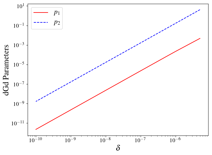
Figure 6: The dGd parameters $p_{1}$ and $p_{2}$ as functions of $\delta$, the main free physical parameter of the scenario.

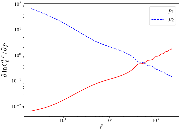
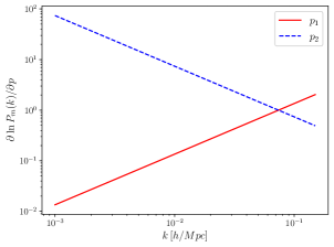
Figure 7: The sensitivity of the CMB temperature power spectrum (top) and matter power spectrum at $z=1$ (bottom) to variations in the two dGd parameters, $p_{1}$ and $p_{2}$.

Given the proposed shape for the power spectrum (Eq. 28), we proceed by assessing the detectability of these fluctuations by CMB and large-scale data.

IV.1 Results

In this section, we study the imprints of dGd parameters on the Planck measurement of the CMB power spectrum (Section IV.1.1) and make a forecast for the detectability of the dGd imprint with future large-scale data. Figure 7 compares the expected impact of the dGd parameters on the CMB (top) and matter power spectrum (bottom) and illustrates where the maximum sensitivity of these observables to the parameters is. It should be noted that $p_{0}$ is hardly distinguishable from the amplitude of primordial inflationary scalar perturbations $A_{\rm s}$ (assuming an almost scale-independent power spectrum). Therefore we do not consider it as a new parameter in our analysis.

IV.1.1 Cosmic Microwave Background

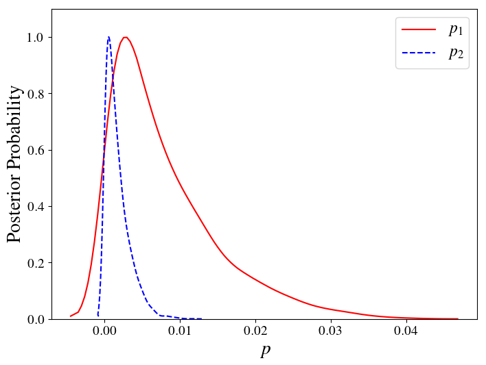
Figure 8: The posterior probability of the dGd parameters $p_{1}$ and $p_{2}$ using Planck dataset.

We modify the publicly available code CosmoMC to take into account the contribution of the dGd induced inhomogeneities as a primordial source of inhomogeneities and leave the dGd parameters $p_{1}$ and $p_{2}$ as free parameters to be estimated by data. We assume uniform priors on these parameters and only require that the total dGd power spectrum, including contribution from both $p_{1}$ and $p_{2}$, be non-negative. Therefore, these two parameters are not separately restricted to non-negative values. As stated before, we use Planck measurement of CMB temperature and polarization anisotropies (Ade et al., 2014). We work in the $\Lambda$CDM theoretical framework, with the only modification possibly coming from the dGd phase transition.

Table 1: Best-fit parameters describing the initial conditions of the universe in the dGd model (both inflationary and dGd parameters) and their $1\sigma$ errors as measured by Planck.

$p_{1}$	$p_{2}$	$n_{\rm s}$	Log$(10^{10}A_{\rm s})$
$0.008^{+0.003}_{-0.008}$	$0.002^{+0.001}_{-0.002}$	$0.9623^{+0.0075}_{-0.0053}$	$3.0410^{+0.0161}_{-0.0239}$

Table 2: Estimated errors on the dGd parameter pair forecasted for future observations of large-scale structure (Euclid, SKA1, and SKA2-like) surveys. In this analysis, the standard cosmological parameters are fixed.

	Euclid-like			SKA1-like			SKA2-like
	GC	WL	total	GC	WL	total	GC	WL	total
$p_{1}$	0.0001	0.0008	0.0001	0.0015	0.0021	0.0011	0.0001	0.0005	0.0001
$p_{2}$	0.0006	0.0016	0.0006	0.0062	0.0027	0.0024	0.0005	0.0009	0.0004

Table 3: Similar to Table 2 but marginalized over the six standard cosmological parameters.

	Euclid-like			SKA1-like			SKA2-like
	GC	WL	total	GC	WL	total	GC	WL	total
$p_{1}$	0.002	0.014	0.002	0.024	0.036	0.014	0.002	0.008	0.001
$p_{2}$	0.003	0.010	0.003	0.033	0.022	0.012	0.003	0.006	0.002

Our parameter set therefore includes the standard cosmological base parameters ($\Omega_{b}h^{2}$, $\Omega_{c}h^{2}$, $\theta$, $\tau$, $A_{s}$ and $n_{s}$, with $k_{\rm pivot}=0.05{\rm Mpc}^{-1}$ as the pivot for scalar perturbations) along with the dGd parameters. We have assumed uniform priors on the dGd parameters, in the range $[0,10]$. We find this prior range to be safe in the sense that it covers all the dGd parameter space with non-negligible likelihood, and the posterior is not cut in the edges of the parameter space due to prior biases. We take the number of relativistic species to be $N_{\nu}=3.046$ and assume the neutrinos to be massless. We have also assumed the primordial tensor perturbations have negligible contribution to CMB temperature and $E$-mode polarization anisotropies. The helium abundance is set from the BBN consistency relation. We use eight chains of parameters and use the Gelman and Rubin R-statistic to assess their convergence. We find that, with a total of about 32000 samples, the chains are converged with $R-1<0.01$.

Table 1 summarizes the results of this dGd-parameter measurement and Figure 8 shows the posterior probabilities of $p_{1}$ and $p_{2}$. The two dGd parameters are almost uncorrelated. That is expected since the two parameters affect different scales. Small scales, or large $k$’s, are most sensitive to $p_{1}$, while large-scales, or small $k$’s, are mostly affected by $p_{2}$ (see equation 28 and Figure 7). The standard parameters also have little correlation with the dGd ones due to the distinct imprints they leave on the power spectrum and are therefore almost unchanged. The results indicate no deviation from the inflationary power-law spectrum in the form predicted by the dGd formalism.

IV.1.2 large-scale Structure

Features in the primordial power spectrum also leave imprints on matter distribution. We investigate the detectability of the dGd-induced features characterized by the two parameters $p_{1}$ and $p_{2}$ in future large-scale surveys. In this work, we make forecast using simulations for the European Space Agency’s Euclid mission, referred to as Euclid-like, and the Square Kilometer Array (SKA), with two different sets of proposed specifications, referred to as SKA1-like and SKA2-like. In particular, we use the weak lensing (WL) and galaxy clustering (GC) probes, following specifications assumed in (Laureijs et al., 2011; Amendola et al., 2013; Santos et al., 2015). We do a Fisher matrix analysis in the linear regime of perturbations assuming a near-Gaussian distribution for the parameter. The formalism and the details of the analysis are similar to the analysis thoroughly described in (Esmaeilian et al., 2021).

Tables 2 and 3 present the forecasted errors of the two dGd parameters for the various experimental scenarios used in this section, for the WL and GC probes, and with the standard cosmological parameters assumed fixed and free respectively. The constraints from GC and WL are tightest from Euclid-like and SKA2-like and comparable to Planck measurements (Table 1).

V Summary and Discussion

In this work, we investigated the observational consequences of a possible phase transition of the spacetime at the end of inflation, the so-called dGd phase transition. We simulated fluctuations in the inflaton field induced by this transition and found the fit to the corresponding power spectrum. The amplitudes of the various terms in the dGd power spectrum were considered as free parameters and were constrained by Planck data. No significant deviations from the standard power-law inflationary power spectrum were found. The high-precision observations of the large-scale structures in the near future could improve these constraints. We made Fisher-based forecasts for Euclid and SKA-like surveys and found comparable bounds on the dGd parameters from the weak lensing and galaxy clustering probes.

If deviations from pure inflationary power law are observed, the consistency of these perturbations with the dGd scenario could be tested by extracting the $\delta$s corresponding to each observed dGd parameter, $p_{1}$ and $p_{2}$, from Figure 6. The agreement of the deduced $\delta$’s (within the error bars) would imply the consistency of the observed deviation as seeded by an early dGd phase transition. The derived value for $\delta$ would also shed light on the physics of the phase transition through constraining its duration $\tilde{t}$ (as discussed in Section IV), which itself depends on the free parameters of the theory $\sigma$, $\lambda$ and $\Lambda$ through Equation 27.

VI Acknowledgement

Part of the numerical computations of this work was carried out on the computing cluster of the Canadian Institute for Theoretical Astrophysics (CITA), University of Toronto.

References

- Davis et al. (1982) M. Davis, J. Huchra, D. W. Latham, and J. Tonry, The Astrophysical Journal 253, 423 (1982).
- Colless et al. (2001) M. Colless, G. Dalton, S. Maddox, W. Sutherland, P. Norberg, S. Cole, J. Bland-Hawthorn, T. Bridges, R. Cannon, C. Collins, et al., Monthly Notices of the Royal Astronomical Society 328, 1039 (2001).
- York et al. (2000) D. G. York, J. Adelman, J. E. Anderson Jr, S. F. Anderson, J. Annis, N. A. Bahcall, J. Bakken, R. Barkhouser, S. Bastian, E. Berman, et al., The Astronomical Journal 120, 1579 (2000).
- Korotky et al. (2020) V. A. Korotky, E. Masár, and Y. N. Obukhov, Universe 6, 14 (2020).
- Bernardeau (1996) F. Bernardeau, Dark Matter in Cosmology Quantam Measurements Experimental Gravitation , 187 (1996).
- Conroy et al. (2005) C. Conroy, A. L. Coil, M. White, J. A. Newman, R. Yan, M. C. Cooper, B. F. Gerke, M. Davis, and D. C. Koo, The Astrophysical Journal 635, 990 (2005).
- Croton and Farrar (2008) D. J. Croton and G. R. Farrar, Monthly Notices of the Royal Astronomical Society 386, 2285 (2008).
- Sousbie et al. (2007) T. Sousbie, C. Pichon, H. Courtois, S. Colombi, and D. Novikov, The Astrophysical Journal 672, L1 (2007).
- Bond et al. (2010) N. A. Bond, M. A. Strauss, and R. Cen, Monthly Notices of the Royal Astronomical Society 409, 156 (2010).
- Choi et al. (2010) E. Choi, N. A. Bond, M. A. Strauss, A. L. Coil, M. Davis, and C. N. Willmer, Monthly Notices of the Royal Astronomical Society 406, 320 (2010).
- Wang et al. (2021) P. Wang, N. I. Libeskind, E. Tempel, X. Kang, and Q. Guo, Nature Astron. 5, 839 (2021), [Erratum: Nature Astron. 5, 1077 (2021)], arXiv:2106.05989 [astro-ph.GA] .
- Lu et al. (2009) T. H.-C. Lu, K. Ananda, C. Clarkson, and R. Maartens, JCAP 02, 023 (2009), arXiv:0812.1349 [astro-ph] .
- Hoyle (1951) F. Hoyle, Problems of cosmical aerodynamics , 195 (1951).
- Peebles (1969) P. J. E. Peebles, Astrophys. J. 155, 393 (1969).
- White (1984) S. D. M. White, Astrophys. J. 286, 38 (1984).
- Porciani et al. (2002) C. Porciani, A. Dekel, and Y. Hoffman, Monthly Notices of the Royal Astronomical Society 332, 325 (2002).
- van de Weygaert et al. (2016) R. van de Weygaert, S. Shandarin, E. Saar, and J. Einasto, The Zeldovich Universe: Genesis and Growth of the Cosmic Web 308 (2016).
- Pichon et al. (2014) C. Pichon, S. Codis, D. Pogosyan, Y. Dubois, V. Desjacques, and J. Devriendt, Proceedings of the International Astronomical Union 11, 421 (2014).
- Kim et al. (2022) Y. Kim, R. Smith, and J. Shin, The Astrophysical Journal 935, 71 (2022).
- Gamow (1946) G. Gamow, Nature 158, 549 (1946).
- Godel (1949) K. Godel, Rev. Mod. Phys. 21, 447 (1949).
- Barrow et al. (1985) J. D. Barrow, R. Juszkiewicz, and D. Sonoda, Monthly Notices of the Royal Astronomical Society 213, 917 (1985).
- Sivaram and Arun (2012) C. Sivaram and K. Arun, (2012).
- Li (1998) L.-X. Li, General Relativity and Gravitation 30, 497 (1998).
- Gangui (2001) A. Gangui, (2001), arXiv:astro-ph/0110285 [astro-ph] .
- Hindmarsh and Kibble (1995) M. B. Hindmarsh and T. W. B. Kibble, Rept. Prog. Phys. 58, 477 (1995), arXiv:hep-ph/9411342 [hep-ph] .
- Vilenkin and Shellard (2000) A. Vilenkin and E. P. S. Shellard, Cosmic Strings and Other Topological Defects (Cambridge University Press, 2000).
- Ade et al. (2014) P. A. R. Ade et al. (Planck), Astron. Astrophys. 571, A25 (2014), arXiv:1303.5085 [astro-ph.CO] .
- Khodabakhshi and Shojai (2015) S. Khodabakhshi and A. Shojai, Phys. Rev. D92, 123541 (2015), arXiv:1603.08241 [gr-qc] .
- Khodabakhshi and Shojai (2017) S. Khodabakhshi and A. Shojai, Eur. Phys. J. C77, 454 (2017), arXiv:1908.07780 [hep-th] .
- Hobson et al. (2006) M. P. Hobson, G. P. Efstathiou, and A. N. Lasenby, General relativity: An introduction for physicists (2006).
- Mukhanov and Winitzki (2007) V. Mukhanov and S. Winitzki, Introduction to quantum effects in gravity (Cambridge University Press, 2007).
- Fursaev and Miele (1994) D. V. Fursaev and G. Miele, Phys. Rev. D49, 987 (1994), arXiv:hep-th/9302078 [hep-th] .
- Elizalde et al. (1994) E. Elizalde, S. D. Odintsov, A. Romeo, A. A. Bytsenko, and S. Zerbini, Zeta regularization techniques with applications (1994).
- Huang (1991) W.-H. Huang, Class. Quant. Grav. 8, 1471 (1991).
- Bordag et al. (2009) M. Bordag, G. L. Klimchitskaya, U. Mohideen, and V. M. Mostepanenko, Advances in the Casimir effect, Vol. 145 (Oxford University Press, 2009).
- Poisson, Eric (2002) Poisson, Eric, An advanced course in general relativity (2002).
- Teukolsky (2015) S. A. Teukolsky, Classical and Quantum Gravity 32, 124006 (2015).
- Rebouças and Tiomno (1983) M. Rebouças and J. Tiomno, Physical Review D 28, 1251 (1983).
- Krasiński (2001) A. Krasiński, Journal of Mathematical Physics 42, 355 (2001).
- Buser et al. (2013) M. Buser, E. Kajari, and W. P. Schleich, New Journal of Physics 15, 013063 (2013).
- Nolan (2020) B. C. Nolan, Classical and Quantum Gravity 37, 085007 (2020).
- Santos and Khanna (2022) A. Santos and F. C. Khanna, Physics Letters B , 137493 (2022).
- Note (1) Https://cosmologist.info/cosmomc/.
- Laureijs et al. (2011) R. Laureijs et al. (EUCLID), (2011), arXiv:1110.3193 [astro-ph.CO] .
- Amendola et al. (2013) L. Amendola, S. Appleby, D. Bacon, T. Baker, M. Baldi, N. Bartolo, A. Blanchard, C. Bonvin, S. Borgani, and et al., Living Reviews in Relativity 16 (2013), 10.12942/lrr-2013-6.
- Santos et al. (2015) M. Santos, P. Bull, D. Alonso, S. Camera, P. Ferreira, G. Bernardi, R. Maartens, M. Viel, F. Villaescusa-Navarro, F. B. Abdalla, and et al., Proceedings of Advancing Astrophysics with the Square Kilometre Array — PoS(AASKA14) (2015), 10.22323/1.215.0019.
- Esmaeilian et al. (2021) M. S. Esmaeilian, M. Farhang, and S. Khodabakhshi, Astrophys. J. 912, 104 (2021), arXiv:2011.14774 [astro-ph.CO] .
- Alexander et al. (2022) S. Alexander, C. Capanelli, E. G. Ferreira, and E. McDonough, Physics Letters B 833, 137298 (2022).
- Motloch et al. (2021) P. Motloch, H.-R. Yu, U.-L. Pen, and Y. Xie, Nature Astronomy 5, 283 (2021).
- Dodelson (2003) S. Dodelson, Modern Cosmology (Academic Press, Amsterdam, 2003).