KUNS-2736

2]Yukawa Institute for Theoretical Physics, Kyoto University, Kyoto 606-8502, Japan

Ab-initio description of excited states of a one-dimensional nuclear matter with the Hohenberg–Kohn-theorem-inspired functional-renormalization-group method

Abstract

We demonstrate for the first time that a functional-renormalization-group aided density-functional theory (FRG-DFT) describes well the characteristic features of the excited states as well as the ground state of an interacting many-body system with infinite number of particles in a unified manner. The FRG-DFT is applied to a $(1+1)$-dimensional spinless nuclear matter. For the excited states, the density–density spectral function is calculated at the saturation point obtained in the framework of FRG-DFT, and it is found that our result reproduces a notable feature of the density–density spectral function of the non-linear Tomonaga-Luttinger liquid: The spectral function has a singularity at the edge of its support of the lower-energy side. These findings suggest that the FRG-DFT is a promising first-principle scheme to analyze the excited states as well as the ground states of quantum many-body systems starting from the inter-particle interaction.

D10, B32, A63

Density-functional theory (DFT) has greatly contributed to our understanding of quantum many-body systems in various fields including quantum chemistry and atomic, molecular, condensed-matter, and nuclear physics; see Refs. coh12 ; lau13 ; mar17 ; jon15 ; nak16 ; dru09 for some recent reviews. The DFT is founded by the Hohenberg-Kohn (HK) theorem hoh64 . The theorem states that the total energy of the system is a functional of the particle density which is a function of single variable $\vec{x}$ and that the variational principle with respect to the density gives the ground-state density and energy exactly. The HK theorem is, however, just an existence theorem, but the DFT or the HK theorem cannot tell us about the energy-density functional (EDF) that we need to minimize. The EDFs employed usually in the practical calculations are thus constructed phenomenologically, and improvement of the EDFs lies at the center in the studies based on DFT. Therefore, it is highly desirable to develop a systematic method to derive the EDF from the underlying microscopic Hamiltonian.

Successful application to the ground state of interacting systems in conjunction with the Kohn-Sham theory koh65 has stimulated attempts to describing excited states and dynamics in a framework of time-dependent DFT (TDDFT) run84 ; lau13 ; nak16 . Presently, the linear-response TDDFT has been successfully applied to the small-amplitude collective modes of excitation, and the real-time TDDFT has been developed to describe even the non-linear dynamics as an initial-value problem. The TDDFT, in principle, can describe the many-body dynamics exactly. It is, however, an open problem to develop a practical method to extract the information of excited states possessing the large-amplitude collective character.

In view of quantum field theory, the two-particle point-irreducible (2PPI) effective action formalism ver92 gives the HK theorem naturally and further the foundation of TDDFT is given in a unified way fuk94 ; val97 . Here, the starting point is a generating functional with a source coupled to the local composite density operator $\hat{\psi}^{\dagger}(\vec{x})\hat{\psi}(\vec{x})$. And then a functional Legendre transformation with respect to the source leads to an effective action of the density, which gives the quantum equation of motion. Therefore, the 2PPI effective action is considered to be a generalization of the EDF.

Let us call here the exact or functional renormalization group (FRG) method wet93 , which is established as a practical way to treat the effective action non-perturbatively and has been successfully applied to quantum many-body problems ber02 ; paw07 ; gie12 ; met12 . The FRG is based on a one-parameter flow equation for the parameter-dependent effective average action, which gives the effective action of a fully-interacting system eventually by taking the quantum fluctuation and correlation gradually starting from a bare system. The 2PPI effective action formalism combined with the FRG thus gives possibly a systematic construction of the EDF based on a microscopic Hamiltonian pol02 ; sch04 ; pol05 ; bra12 ; kem13 ; kem17 ; kem17b ; ram17 ; we call such an approach the functional-renormalization-group aided density-functional theory (FRG-DFT). This approach can be a promising scheme for solving the fundamental problems in DFT and providing further insights in understanding the many-body systems.

The FRG-DFT method has been applied to a zero-dimensional model of anharmonic vibrator kem13 ; lia18 , and a one-dimensional quantum anharmonic vibrator kem13 to show the feasibility and effectiveness. The estimation of uncertainty due to the truncation was given and an effective way to treat the higher-order correction was proposed lia18 . The FRG-DFT method has also been applied to a (1+1)-dimensional many-body model simulating one-dimensional nucleons with a fixed particle-number formalism kem17 , although the bound-state energy was underestimated by approximately 30% in comparison with the exact solution in two-particle system and over 17% in comparison with the results obtained using the Monte Carlo method ale89 when the number of particles is no more than eight. In addition, the study of (1+1)-dimensional systems composed of finite number of spin-1/2 fermions interacting via a contact interaction has been reported kem17b ; ram17 .

Since the 2PPI effective action is an effective action which is by definition capable of describing time-dependent phenomena as well as static phenomena equally, the FRG-DFT method should be in principle applicable to not only the ground state but also the excited sates though there have been no attempts to demonstrate it as far as we are aware of. It should be noted here that the FRG has been applied to obtain the spectral functions in the $O(N)$ model kam14 and the quark-meson model tri14a ; tri14b ; yok16 ; yok17 . Here, the analytic continuation is taken at each order before evaluation of the flow equations. This technique is thus much easier numerically than the standard method such as the maximum entropy method or the Padé approximation.

In this Letter, we demonstrate for the first time that our FRG-DFT works well for describing the excited states as well as the ground states of continuum matter. We are going to consider a (1+1)-dimensional spinless nuclear matter ale89 with infinite number of particles. After summarizing our result for the ground state energy yok18 where the resultant equation of state was found to give the saturation energy compatible with that obtained using the Monte Carlo method ale89 , we show the numerical result for the density–density spectral function. We find that our density–density spectral function reproduces the existence of the peak at the edge of its support in the lower-energy side, which is known as a notable feature of the non-linear Tomonaga–Luttinger liquid. Our result suggests that the FRG-DFT is a powerful way to analyze excited states as well as ground states of quantum many-body systems.

For self-containedness,we first recapitulate some part of our FRG-DFT formalism to analyze the ground state properties of infinite matters, which has been developed by the present authors in Ref. yok18 .

A microscopic input in our study is the inter-particle interaction. The interaction we adopted consists of the short-range repulsive core and the long-range attractive force of ‘nucleons’ both of which are given by a Gaussian : $U(r)=({g}/\sqrt{\pi})(\sigma_{1}^{-1}{\rm e}^{-r^{2}/\sigma_{1}^{2}}-\sigma_{2}^{-1}{\rm e}^{-r^{2}/\sigma_{2}^{2}})$, where $\sigma_{1}>0$, $\sigma_{2}>0$ and $g>0$. As given in Ref. ale89 , we chose $g=12$, $\sigma_{1}=0.2$ and $\sigma_{2}=0.8$ in units such that the mass of a nucleon is 1. These values were determined under the assumptions that the relevant dimensionless values in one dimension are comparable with the empirical ones in three dimensions.

Although we are primarily interested in the system with zero-temperature in the present work, we found that the use of the finite-temperature imaginary-time formalism is most convenient. Then the action of the one-dimensional interacting spinless fermions reads

$$S[\psi^{*},\psi]=\int_{\chi}\psi^{*}(\chi)\left(\partial_{\tau}-\frac{1}{2}\partial^{2}_{x}\right)\psi(\chi)+\frac{1}{2}\int_{\chi,\chi^{\prime}}\psi^{*}(\chi)\psi^{*}(\chi^{\prime})U_{\rm 2b}(\chi,\chi^{\prime})\psi(\chi^{\prime})\psi(\chi),$$ (1)

where we have introduced the shorthands $\chi=(\tau,x)$, $\int_{\chi}=\int_{-\beta/2}^{\beta/2}d\tau\int dx$ and $U_{\rm 2b}(\chi,\chi^{\prime}):=U_{\rm 2b}(\chi-\chi^{\prime}):=\delta(\tau-\tau^{\prime})U(x-x^{\prime})$.

Since we are going to employ the techniques developed in the FRG method, we regulated the interaction between fermions by multiplying $U_{\rm 2b}(\chi,\chi^{\prime})$ by a regulator function $\mathcal{R}_{\lambda}(\tau,x,\tau^{\prime},x^{\prime})$ as introduced in Refs. pol02 ; sch04 ; kem17 , and the resulting regulated action is given as

$$S_{\lambda}[\psi^{*},\psi]=\int_{\chi}\psi^{*}(\chi)\left(\partial_{\tau}-\frac{1}{2}\partial^{2}_{x}\right)\psi(\chi)+\frac{1}{2}\int_{\chi,\chi^{\prime}}\psi^{*}(\chi)\psi^{*}(\chi^{\prime})\mathcal{R}_{\lambda}(\chi,\chi^{\prime})U_{\rm 2b}(\chi,\chi^{\prime})\psi(\chi^{\prime})\psi(\chi).$$ (2)

Here, $\mathcal{R}_{\lambda}(\chi,\chi^{\prime})$ was chosen so as to satisfy the following conditions: $\lim_{\lambda\rightarrow 0}\mathcal{R}_{\lambda}(\chi,\chi^{\prime})=0$ and $\lim_{\lambda\rightarrow 1}\mathcal{R}_{\lambda}(\chi,\chi^{\prime})=1$. Under these conditions, $S_{\lambda}$ becomes the action of free particles at $\lambda=0$ and that of interacting particles at $\lambda=1$, namely Eq. (1). Specifically, we chose $\mathcal{R}_{\lambda}(\chi_{1},\chi_{2})=\lambda$ for simplicity pol02 ; sch04 . We then define the $\lambda$-dependent generating functional for density-density correlation functions as $Z_{\lambda}[J]=\int\mathcal{D}\psi^{*}\mathcal{D}\psi\exp(-S_{\lambda}[\psi^{*},\psi]+\int_{\chi}J(\chi)\hat{\rho}(\chi))$ with $\hat{\rho}(\chi)=\psi^{*}(\chi)\psi(\chi)$ being the composite local number density operator. The generating functional for the connected density correlation functions $G_{\lambda}^{(n)}(\chi_{1},\cdots,\chi_{n})$ is given as $W_{\lambda}[J]=\ln Z_{\lambda}[J]$, i.e. $G_{\lambda}^{(n)}(\chi_{1},\cdots,\chi_{n})=\delta^{n}W_{\lambda}[J]/\delta J(\chi_{1})\cdots\delta J(\chi_{n})|_{J=0}$.

Then the effective action $\Gamma_{\lambda}[\rho]$ of the local density $\rho(\chi)$ is obtained by the Legendre transformation of $W_{\lambda}[J]$: $\Gamma_{\lambda}[\rho]=\sup_{J}(-W_{\lambda}[J]+\int_{\chi}J(\chi)\rho(\chi))$. An important feature of $\Gamma_{\lambda}[\rho]$ is that it can be related to the energy density functional $E_{\lambda}[\rho]$ as $E_{\lambda}[\rho]=\lim_{\beta\rightarrow\infty}\Gamma_{\lambda}[\rho]/\beta$ fuk94 , i.e. the ground state density $\rho_{\rm gs,\lambda}(\chi)$ and energy $E_{\rm gs,\lambda}$ are obtained variationally from $\Gamma_{\lambda}[\rho]$. When considering the variational problem under the constraint that the particle number is set to some value, we should minimize $I_{\lambda}[\rho]:=\Gamma_{\lambda}[\rho]-\mu_{\lambda}\int_{\chi}\rho(\chi)$ with respect to $\rho(\chi)$. Here, we have introduced a $\lambda$-dependent chemical potential $\mu_{\lambda}$ to control the change of the particle number during the flow caused by switching on of the interaction yok18 . In this case, the ground state density $\rho_{\rm gs,\lambda}(\chi)$ satisfies the following stationary condition: $(\delta\Gamma_{\lambda}/\delta\rho(\chi))[\rho_{\rm gs,\lambda}]=\mu_{\lambda}$. Here, we should mention that the chemical potential depending on the RG parameter was studied hon01 ; vil17 in the framework of the functional RG à la Wetterich wet93 and the change of the chemical potential by the presence of interaction was discussed in the context of DFT dru09 .

The renormalization group flow equation of $\Gamma_{\lambda}[\rho]$ reads sch04 ; kem17

$$\partial_{\lambda}\Gamma_{\lambda}[\rho]=\frac{1}{2}\int_{\chi_{1},\chi_{2}}U_{\rm 2b}(\chi_{1},\chi_{2})\left(\rho(\chi_{1})\rho(\chi_{2})+\left(\frac{\delta^{2}\Gamma_{\lambda}[\rho]}{\delta\rho\delta\rho}\right)^{-1}(\chi_{1},\chi_{2})-\rho(\chi_{2})\delta(x_{2}-x_{1})\right).$$ (3)

One can calculate the effective action $\Gamma_{\lambda=1}[\rho]$, whose classical action is given in Eq. (1), by solving Eq. (3) with the initial condition $\Gamma_{\lambda=0}[\rho]$, which is the effective action of the non-interacting system. The functional differential equation (3) can be converted to an infinite series of differential equations by the expansion around $\rho=\rho_{\rm gs,\lambda}$. In particular, from Eq. (3) and its second derivative around $\rho=\rho_{\rm gs,\lambda}$, and the stationary condition, the flow equations of the energy $E_{\rm gs,\lambda}$, the density $\rho_{\rm gs,\lambda}$ at the ground state, and the two-point correlation function $G_{\lambda}^{(2)}(\chi,\chi^{\prime})$ are obtained as follows:

$$\partial_{\lambda}E_{\rm gs,\lambda}= \lim_{\beta\to\infty}\frac{1}{\beta}\left[\int_{\chi}\mu_{\lambda}\partial_{\lambda}\rho_{\rm gs,\lambda}(\chi)\right.$$

$$+\left.\frac{1}{2}\int_{\chi,\chi^{\prime}}U_{\rm 2b}(\chi,\chi^{\prime})\left(\rho_{\rm gs,\lambda}(\chi)\rho_{\rm gs,\lambda}(\chi^{\prime})+G_{\lambda}^{(2)}(\chi,\chi^{\prime})-\rho_{\rm gs,\lambda}(\chi^{\prime})\delta(x^{\prime}-x)\right)\right],$$ (4)

$$\partial_{\lambda}\rho_{\rm gs,\lambda}(\chi)= -\frac{1}{2}\int_{\chi_{1},\chi_{2}}U_{\rm 2b}(\chi_{1},\chi_{2})G_{\lambda}^{(3)}(\chi_{2},\chi_{1},\chi)$$

$$+\int_{\chi_{1}}G_{\lambda}^{(2)}(\chi,\chi_{1})\left(\partial_{\lambda}\mu_{\lambda}-\int_{\chi_{2}}U_{\rm 2b}(\chi_{1},\chi_{2})\rho_{\rm gs,\lambda}(\chi_{2})+\frac{1}{2}U(0)\right),$$ (5)

$$\partial_{\lambda}G_{\lambda}^{(2)}(\chi,\chi^{\prime})= -\int_{\chi_{1},\chi_{2}}U_{\rm 2b}(\chi_{1},\chi_{2})\left(G_{\lambda}^{(2)}(\chi,\chi_{1})G_{\lambda}^{(2)}(\chi_{2},\chi^{\prime})+\frac{1}{2}G_{\lambda}^{(4)}(\chi_{2},\chi_{1},\chi,\chi^{\prime})\right)$$

$$+\int_{\chi_{1}}G_{\lambda}^{(3)}(\chi,\chi^{\prime},\chi_{1})\left(\partial_{\lambda}\mu_{\lambda}-\int_{\chi_{2}}U_{\rm 2b}(\chi_{1},\chi_{2})\rho_{\rm gs,\lambda}(\chi_{2})+\frac{1}{2}U(0)\right).$$ (6)

In this Letter, we assume that the ground state of the system is homogeneous for any $\lambda$. In this case, we can set $\rho_{\rm gs,\lambda}$ to a constant value during the flow, i.e. $\partial_{\lambda}\rho_{\rm gs,\lambda}=0$, by choosing $\mu_{\lambda}$ so as to satisfy $\partial_{\lambda}\mu_{\lambda}=\tilde{U}(0)\rho_{\rm gs,\lambda}-U(0)/2+\int_{P}\tilde{U}(p)\tilde{G}_{\lambda}^{(3)}(P,-P)/(2\tilde{G}_{\lambda}^{(2)}(0))$. Here, for convenience we have introduced the momentum representations $\tilde{U}(p):=\int_{x}U(x)e^{-ipx}$ and $(2\pi)^{2}\delta(P_{1}+\cdots+P_{n})\tilde{G}_{\lambda}^{(n)}(P_{1},\cdots,P_{n-1}):=\int_{\chi_{1},\cdots,\chi_{n}}e^{-i(P_{1}\cdot\chi_{1}+\cdots+P_{n}\cdot\chi_{n})}G_{\lambda}^{(n)}(\chi_{1},\cdots,\chi_{n})$, where $P_{i}:=(\omega_{i},p_{i})$ is a vector of a Matsubara frequency and a momentum, and the short hand $\int_{P}:=\int dpd\omega/(2\pi)^{2}$. We note that $\tilde{G}_{\lambda}^{(2)}(0)$ is interpreted as the $p$ limit of $\tilde{G}_{\lambda}^{(2)}(P)$, i.e. $\lim_{p\to 0}\tilde{G}_{\lambda}^{(2)}(0,p)$, in our case and thus is regarded as the static particle-density susceptibility for75 ; kun91 ; fuj04 ; yok18 , which is usually nonzero. Under the choice of $\mu_{\lambda}$, Eqs. (4) and (6) are reduced to the following equations, respectively yok18 :

$$\partial_{\lambda}\overline{E}_{\rm gs,\lambda}= \frac{\rho_{\rm gs,0}}{2}\tilde{U}(0)+\frac{1}{2\rho_{\rm gs,0}}\int_{p}\tilde{U}(p)\left(\int_{\omega}\tilde{G}^{(2)}_{\lambda}(P)-\rho_{\rm gs,0}\right),$$ (7)

$$\partial_{\lambda}\tilde{G}_{\lambda}^{(2)}(P)= -\tilde{U}(p)\tilde{G}_{\lambda}^{(2)}(P)^{2}-\frac{1}{2}\int_{P^{\prime}}\tilde{U}(p^{\prime})\left[\tilde{G}^{(4)}_{\lambda}(P^{\prime},-P^{\prime},P)-\frac{\tilde{G}_{\lambda}^{(3)}(P^{\prime},-P^{\prime})\tilde{G}_{\lambda}^{(3)}(P,-P)}{\tilde{G}_{\lambda}^{(2)}(0)}\right],$$ (8)

where we have introduced the energy per particle $\overline{E}_{\rm gs,\lambda}=E_{\rm gs,\lambda}/\int dx\rho_{\rm gs,0}$.

Equation (8) contains $\tilde{G}^{(3,4)}_{\lambda}$, the flow equations for which are derived from Eq. (3) in terms of $\tilde{G}^{(n\geq 5)}_{\lambda}$ and so on because the flow equation for $\tilde{G}^{(n)}_{\lambda}$ depends on $\tilde{G}^{(2)}_{\lambda},\cdots,\tilde{G}^{(n+2)}_{\lambda}$. Thus it is obvious that a truncation scheme is necessary for solving the flow equations in a practical calculation. In the present calculation, we did not consider the flows of $\tilde{G}^{(3,4)}_{\lambda}$. However, the simple replacement of $\tilde{G}^{(3,4)}_{\lambda}$ by $\tilde{G}^{(3,4)}_{0}$ in Eq. (8) causes the breaking of the Pauli exclusion principle. To avoid this artifact, we used the following approximation as introduced in Ref. kem17 :

$$\int_{P^{\prime}}\tilde{U}(p^{\prime})\left[\tilde{G}^{(4)}_{\lambda}(P^{\prime},-P^{\prime},P)-\tilde{G}_{\lambda}^{(3)}(P^{\prime},-P^{\prime})\tilde{G}_{\lambda}^{(3)}(P,-P)\tilde{G}_{\lambda}^{(2)}(0)^{-1}\right]$$

$$\approx f_{\cal P}(\lambda)\int_{P^{\prime}}\tilde{U}(p^{\prime})\left[\tilde{G}^{(4)}_{0}(P^{\prime},-P^{\prime},P)-\tilde{G}_{0}^{(3)}(P^{\prime},-P^{\prime})\tilde{G}_{0}^{(3)}(P,-P)\tilde{G}_{0}^{(2)}(0)^{-1}\right],$$ (9)

with $f_{\cal P}(\lambda)$ being a factor to preserve the effect of Pauli blocking. According to the Pauli blocking, we have $\partial_{\lambda}G_{\lambda}^{(2)}(\chi,\chi)=0$. Therefore $f_{\cal P}(\lambda)$ is determined using Eq. (8): $f_{\cal P}(\lambda)=-2\int_{P}\tilde{U}(p)\tilde{G}_{\lambda}^{(2)}(P)^{2}/\int_{P^{\prime},P^{\prime\prime}}\tilde{U}(p^{\prime})[\tilde{G}^{(4)}_{0}(P^{\prime},-P^{\prime},P^{\prime\prime})-\tilde{G}_{0}^{(3)}(P^{\prime},-P^{\prime})\tilde{G}_{0}^{(3)}(P^{\prime\prime},-P^{\prime\prime})\tilde{G}_{0}^{(2)}(0)^{-1}].$ At $\lambda=0$, we have $f_{\cal P}(0)=1$.

To solve the flow equations (7) and (8), we need the initial conditions $\overline{E}_{\rm gs,\lambda=0}$, $\rho_{\rm gs,\lambda=0}$, and $\tilde{G}^{(2,3,4)}_{\lambda=0}$. We denote $\rho_{\rm gs,0}$ by $n$, which is always the density of the ground state during the flow, and in particular at $\lambda=1$, because $\rho_{\rm gs,\lambda}(\chi)=\rho_{\rm gs,0}$. Then the Fermi momentum and Fermi energy are defined as $p_{\rm F}=\pi n$ and $E_{\rm F}=p_{\rm F}^{2}/2$, respectively. $\overline{E}_{\rm gs,\lambda=0}$ is the ground state energy of the one-dimensional free Fermi gas: $\overline{E}_{\rm gs,0}=E_{\rm F}/3$. $G^{(2,3,4)}_{\lambda=0}$ are the correlation functions for free particles:

$$G^{(2)}_{0}(P)= -\int_{P^{\prime}}G_{\rm F,0}^{(2)}(P+P^{\prime})G_{\rm F,0}^{(2)}(P^{\prime}),$$ (10)

$$\tilde{G}^{(3)}_{0}(P_{1},P_{2})= -\sum_{\sigma\in S_{2}}\int_{P^{\prime}}\tilde{G}_{\rm F,0}^{(2)}(P^{\prime})\tilde{G}_{\rm F,0}^{(2)}(P_{\sigma(1)}+P^{\prime})\tilde{G}_{\rm F,0}^{(2)}(P_{\sigma(1)}+P_{\sigma(2)}+P^{\prime}),$$ (11)

$$G^{(4)}_{0}(P_{1},P_{2},P_{3})= -\sum_{\sigma\in S_{3}}\int_{P^{\prime}}G_{\rm F,0}^{(2)}(P^{\prime})G_{\rm F,0}^{(2)}(P_{\sigma(1)}+P^{\prime})G_{\rm F,0}^{(2)}(P_{\sigma(1)}+P_{\sigma(2)}+P^{\prime})$$

$$\times G_{\rm F,0}^{(2)}(P_{\sigma(1)}+P_{\sigma(2)}+P_{\sigma(3)}+P^{\prime}).$$ (12)

Here $S_{2}$ and $S_{3}$ are the symmetric groups of order two and three, respectively, and $G_{\rm F,0}^{(2)}(P)$ is the two-point propagator of free fermions: $G_{\rm F,0}^{(2)}(P)={1}/(-i\omega+\epsilon(p))$, where $\epsilon(p):=p^{2}/2-E_{\rm F}$. Using Eqs. (10)-(12), the expressions of the flow equations (7) and (8) under the approximation Eq. (9) are found to be the same as those obtained from the continuum limit of the system with finite number of particles in a finite box presented in Ref. kem17 .

We need to evaluate the momentum integrals such as $\int dp^{\prime}\tilde{U}(p^{\prime})/p^{\prime}$, which appear in the second term in the right-hand side of Eq. (8). The integrand apparently has a singular point at $p^{\prime}=0$, which is actually absent because $\tilde{U}(0)=0$ in the present case. In order to avoid a division-by-zero operation, we rewrote the integrand by using the Maclaurin expansion of $\tilde{U}(p^{\prime})$ at small $p^{\prime}$ to a manifestly regular form for the numerical calculation.

The results for the equation of state and the saturation energy, and the comparison with the Monte Carlo simulation ale89 were shown in Ref. yok18 . A remark is in order here: In the Monte Carlo simulation, the saturation energy was mere an extrapolated energy at a given density $n=1.16$, which is considered to be close ale89 but not equal to the saturation density; moreover the extrapolation was made from the results for finite particle systems with a particle number up to 12. In contrast, our FRG-DFT calculation was made for the system with infinite number of particles, and the density was varied continuously. The saturation energy derived from FRG-DFT is quite close to the result of the Monte Carlo simulation: We found that the discrepancy between the saturation energy given by FRG-DFT and that by the Monte Carlo simulation is 2.7%. We pointed out that such an accuracy was acquired with little computational time or resources in our framework of FRG-DFT.

This successful application to the ground-state properties of a many-body system rouses one’s interest in extension of FRG-DFT to describing excited states. Then we are going to describe our way to calculate the density–density spectral function. We define the density–density spectral function $\rho_{\rm d,\lambda}(\omega,p)$ as $\rho_{\rm d,\lambda}(\omega,p)=-2\mathrm{Im}\tilde{G}_{\rm R,\lambda}^{(2)}(\omega,p)$, where $\tilde{G}^{(2)}_{\rm R,\lambda}(\omega,p)$ is the retarded two-point density correlation function, which is obtained from the analytic continuation of $\tilde{G}^{(2)}_{\lambda}(\omega_{\rm I},p)$: $\tilde{G}^{(2)}_{\rm R,\lambda}(\omega,p)=-\tilde{G}^{(2)}_{\rm ana,\lambda}(\omega+i\epsilon,p)$. Here, $\epsilon$ is a positive infinitesimal and $\tilde{G}^{(2)}_{\rm ana,\lambda}(z,p)$ is a complex function of $z\in\mathbb{C}$ which is regular in the upper-half plane of $z$ and satisfies $\tilde{G}^{(2)}_{\rm ana,\lambda}(-i\omega_{\rm I},p)=\tilde{G}^{(2)}_{\lambda}(\omega_{\rm I},p)$ for $\omega_{\rm I}\in\mathbb{R}$. The analytic continuation to obtain $\tilde{G}^{(2)}_{\rm ana,\lambda}(z,p)$ from $\tilde{G}^{(2)}_{\lambda}(\omega_{\rm I},p)$ is often an obstruction for a numerical analysis. In our case, however, the analytic continuation can be performed in the level of the flow equations as in Refs. kam14 ; tri14a ; tri14b ; yok16 ; yok17 , which is much easier numerically than the standard procedures such as the maximum entropy method or the Páde approximation. Under the approximation Eq. (9), one finds that the second term of Eq. (8) is regular in the upper-half plane of $z$ when $P^{0}$ is simply replaced with $-iz$. Then $\tilde{G}_{\lambda}^{(2)}(P)|_{P^{0}\rightarrow-iz}$ also keeps regular in the upper-half of $z$ during the flow. Therefore, we have the flow equation for $\tilde{G}^{(2)}_{\rm R,\lambda}(\omega,p)$:

$$\partial_{\lambda}\tilde{G}_{\rm R,\lambda}^{(2)}(\omega,p)\approx \tilde{U}(p)\tilde{G}_{\rm R,\lambda}^{(2)}(\omega,p)^{2}$$

$$+\frac{f_{\cal P}(\lambda)}{2}\int_{P^{\prime}}\tilde{U}(p^{\prime})\left.\left[\tilde{G}^{(4)}_{0}(P^{\prime},-P^{\prime},P)-\frac{\tilde{G}_{0}^{(3)}(P^{\prime},-P^{\prime})\tilde{G}_{0}^{(3)}(P,-P)}{\tilde{G}_{0}^{(2)}(0)}\right]\right|_{P^{0}\rightarrow-i(\omega+i\epsilon)}.$$ (13)

The initial condition of this flow equation $\tilde{G}_{\rm R,0}^{(2)}(\omega,p)$ is given by the replacement of $P^{0}$ with $-i(\omega+i\epsilon)$ in Eq. (10). As discussed below, the contribution from the second term in the right-hand side of the flow equation (13) is important to capture the feature of the spectral function in (1+1) dimensions. If the second term of the right-hand side of Eq. (13) is neglected, this flow equation can be solved analytically: We have $\tilde{G}_{\rm R,\lambda=1}^{(2)}(\omega,p)=(\tilde{G}_{\rm R,0}^{(2)}(\omega,p)^{-1}-U(p))^{-1}$, which is equivalent to that derived in the random phase approximation (RPA).

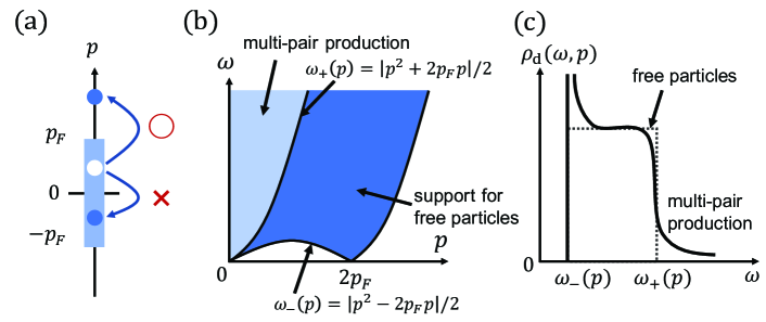
Figure 1: (a) Schematic picture of the particle–hole excitation from the Fermi sphere. Due to the Pauli blocking, some excitations are forbidden kinematically, which gives the lower bound of the energy of the support of the density–density spectral function $\omega_{-}(p)$ in $0\leq p\leq p_{\rm F}$. (b) The supports of the spectral functions for the interacting case and free case. The support in $\omega>\omega_{+}(p)$ is due to the contribution from multi-pair productions. (c) The expected $\omega$ dependence of $\rho_{\rm d}(\omega,p)$ at a fixed $p$ in the interacting case (solid line) and free case (dotted line).

Before presenting our result of the density–density spectral function $\rho_{\rm d}(\omega,p)$, we briefly mention the expected behavior of the density–density spectral function of (1+1)-dimensional interacting fermions. First, let us consider the free fermion case. If the particle–hole excitation with an energy $\omega$ and a momentum $p$ is kinematically forbidden, $\rho_{\rm d}(\omega,p)$ is zero. For (1+1)-dimensional free fermions, a particle–hole excitation with an energy $\omega$ and a momentum $p$ is kinematically allowed if the following condition is satisfied: $\omega_{-}(p)\leq\omega\leq\omega_{+}(p)$, where $\omega_{-}(p):=|p^{2}-2p_{\rm F}p|/2$ and $\omega_{+}(p):=|p^{2}+2p_{\rm F}p|/2$; see Fig. 1(a). Therefore $\rho_{\rm d}(\omega,p)$ has its support as shown in Fig. 1(b). On this support, the strength of $\rho_{\rm d}(\omega,p)$ does not depend on $\omega$: $\rho_{\rm d}(\omega,p)=p^{-1}$.

Then we consider the interacting fermions. To analyze $\rho_{\rm d}(\omega,p)$ for interacting fermions, the inclusion of the nonlinearity of the fermionic dispersion relation is crucial pus06 , which is not taken into account in the Tomonaga–Luttinger (TL) model tom50 ; lut63 . The bosonization scheme taking the nonlinearity into account has been developed pus06 ; teb07 ; ima12 and predicted that the qualitative behavior of $\rho_{\rm d}(\omega,p)$ drastically deviates from that in the case of free particles: First, $\rho_{\rm d}(\omega,p)$ has power-law singularities at the edge of its support of the lower-energy side $\omega=\omega_{-}(p)$. These singularities emerge due to the same mechanism as the singularity appearing in the X-ray absorption rate of metals noz69 ; mah00 , which is caused by the proliferation of low-energy particle-hole pairs. Second, $\rho_{\rm d}(\omega,p)$ exhibits power-law suppression at $\omega=\omega_{+}(p)$ and the support is broaden to $\omega>\omega_{+}(p)$ because of the contribution from the multi-pair productions. The expected shape of the strength of $\rho_{\rm d}(\omega,p)$ is schematically illustrated in Fig. 1(c).

Let us discuss our numerical results of $\rho_{\rm d}(\omega,p)$. We set the density to that at the saturation point derived from FRG-DFT: $n=\rho_{\rm s}=1.20$ yok18 . Figure 2 shows the contour map of $\rho_{\rm d}(\omega,p)$ on the $(\omega,p)$-plane. Our spectral function has the same support as that for the free fermions, which is in contradiction to the expectation that $\rho_{\rm d}(\omega,p)$ has support in $\omega>\omega_{+}(p)$. This is possibly due to the approximation made in Eq. (9), where the contribution from the multi-pair diagrams is discarded. To include the contribution from the multi-pair diagrams, the flow of the four point correlation function is needed to be considered, though which is beyond the scope of this Letter.

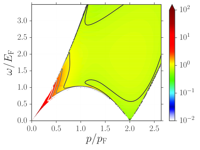
Figure 2: The contour map of the density–density spectral function on the $(\omega,p)$-plane.

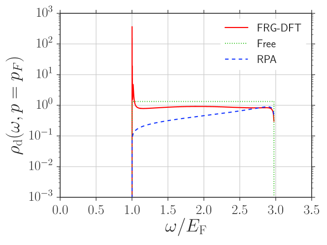
Figure 3: The $\omega$ dependence of the density–density spectral function when the momentum is fixed to $p=p_{\rm F}$. The results of the FRG-DFT (solid red line), free particles (green dotted line) and the RPA (blue dashed line) are shown.

Shown in Fig. 3 is the spectral function $\rho_{\rm d}(\omega,p)$ at a fixed momentum $p=p_{\rm F}$. The results of the RPA and the case of free fermions are also shown for comparison. The spectral function obtained by FRG-DFT reveals the existence of a peak at $\omega=\omega_{-}(p_{\rm F})$ in contrast to that derived from the RPA. A key ingredient for such a peak to emerge is the contribution from the second term in the right-hand side in Eq. (13), which is not included in the RPA. This term has singularities at $\omega=\omega_{-}(p_{\rm F})$, which gives the peak structure in $\rho_{\rm d}(\omega,p)$. In the very close region to $\omega=\omega_{-}(p)$, we found that the spectral function is split into some peaks with slightly different energies, which is different from a simple power-law singularity.

Summarizing the paper, we demonstrated how the FRG-DFT analysis of the ground and excited states works in a one-dimensional continuum spinless nuclear matter. We obtained the saturation energy from the resultant equation of state, which differs from that obtained using the Monte Carlo simulation by only 2.7%. Moreover, we reproduced a notable feature of the one-dimensional fermion system that the density–density spectral function has singularities at the edge of its support of the lower-energy side. Therefore, our result suggests that the FRG-DFT is a promising way for the analysis of not only ground states but also excited states of the quantum many-body systems. The FRG-DFT is expected to be adapted to various systems because our formalism can be naturally extended to higher-dimensional systems, and systems with internal degrees of freedom kem17b ; ram17 , superfluidity, and finite temperature.

There showed up, however, some unexpected behaviors in our result of the density–density spectral function. At higher-energy side, the broadening of the support of the spectral due to the multi-pair production has not appeared in the present framework. This would be because we miss the contribution from the multi-pair production by ignoring the flow of the four-point correlation function. In addition, the spectral function was unexpectedly split into some peaks with slightly different energies in the very close region to the edge of its support of the lower-energy side. The inclusion of the flows of higher-order correlation functions or the use of other approximation schemes such as the KS-FRG lia18 is an important future work to see whether these are due to the approximations and/or truncations employed.

Describing the non-uniform systems is another interesting direction. The introduction of a non-uniform chemical potential can realize such systems. Our flow equations (4)-(6) are straightforwardly extended to the case of non-uniform chemical potential and can be used to analyze non-uniform systems.

We thank Jean-Paul Blaizot for his interest in and critical and valuable comments on the present work. We also acknowledge Christof Wetterich, Jan M. Pawlowski and Jochen Wambach for their interest in and fruitful comments on the present work. T. Y. was supported by the Grants-in-Aid for JSPS fellows (Grant No. 16J08574). K. Y. was supported by the JSPS KAKENHI (Grant No. 16K17687). T. K. was supported by the JSPS KAKENHI Grants (Nos. 16K05350 and 15H03663) and by the Yukawa International Program for Quark-Hadron Sciences (YIPQS).

References

- (1) Aron J. Cohen, Paula Mori-Sánchez, and Weitao Yang, Chemical Reviews, 112(1), 289–320, PMID: 22191548 (2012), https://doi.org/10.1021/cr200107z.
- (2) Adèle D. Laurent and Denis Jacquemin, International Journal of Quantum Chemistry, 113(17), 2019–2039 (2013).
- (3) Narbe Mardirossian and Martin Head-Gordon, Molecular Physics, 115(19), 2315–2372 (2017), https://doi.org/10.1080/00268976.2017.1333644.
- (4) R. O. Jones, Rev. Mod. Phys., 87, 897–923 (2015).
- (5) Takashi Nakatsukasa, Kenichi Matsuyanagi, Masayuki Matsuo, and Kazuhiro Yabana, Rev. Mod. Phys., 88, 045004 (2016).
- (6) J. E. Drut, R. J. Furnstahl, and L. Platter, Prog. Part. Nucl. Phys., 64, 120–168 (2010), arXiv:0906.1463.
- (7) P. Hohenberg and W. Kohn, Phys. Rev., 136, B864–B871 (1964).
- (8) W. Kohn and L. J. Sham, Phys. Rev., 140, A1133–A1138 (1965).
- (9) Erich Runge and E. K. U. Gross, Phys. Rev. Lett., 52, 997–1000 (1984).
- (10) Henri Verschelde and Marnix Coppens, Physics Letters B, 287(1), 133 – 137 (1992).
- (11) Reijiro Fukuda, Takao Kotani, Yoko Suzuki, and Satoshi Yokojima, Progress of Theoretical Physics, 92(4), 833–862 (1994).
- (12) M. Valiev and G. W. Fernando, eprint arXiv:cond-mat/9702247 (1997), cond-mat/9702247.
- (13) Christof Wetterich, Phys. Lett., B301, 90–94 (1993).
- (14) Juergen Berges, Nikolaos Tetradis, and Christof Wetterich, Phys. Rept., 363, 223–386 (2002), arXiv:hep-ph/0005122.
- (15) Jan M. Pawlowski, Annals Phys., 322, 2831–2915 (2007), arXiv:hep-th/0512261.
- (16) Holger Gies, Lect. Notes Phys., 852, 287–348 (2012), arXiv:hep-ph/0611146.
- (17) Walter Metzner, Manfred Salmhofer, Carsten Honerkamp, Volker Meden, and Kurt Schönhammer, Rev. Mod. Phys., 84, 299–352 (2012).
- (18) J. Polonyi and K. Sailer, Phys. Rev., B66, 155113 (2002), arXiv:cond-mat/0108179.
- (19) A. Schwenk and J. Polonyi, Towards density functional calculations from nuclear forces, In 32nd International Workshop on Gross Properties of Nuclei and Nuclear Excitation: Probing Nuclei and Nucleons with Electrons and Photons (Hirschegg 2004) Hirschegg, Austria, January 11-17, 2004, pages 273–282 (2004), arXiv:nucl-th/0403011.
- (20) J. Polonyi and K. Sailer, Phys. Rev. D, 71, 025010 (Jan 2005).
- (21) Jens Braun, J. Phys., G39, 033001 (2012), arXiv:1108.4449.
- (22) Sandra Kemler and Jens Braun, J. Phys., G40, 085105 (2013), arXiv:1304.1161.
- (23) Sandra Kemler, Martin Pospiech, and Jens Braun, J. Phys., G44(1), 015101 (2017), arXiv:1606.04388.
- (24) Sandra Karina Kemler, From Microscopic Interactions to Density Functionals, PhD thesis, Technische Universität, Darmstadt (2017).
- (25) Lukas Rammelmüller, William J. Porter, Joaquín E. Drut, and Jens Braun, Phys. Rev. D, 96, 094506 (Nov 2017).
- (26) Haozhao Liang, Yifei Niu, and Tetsuo Hatsuda, Phys. Lett., B779, 436–440 (2018), arXiv:1710.00650.
- (27) C. Alexandrou, J. Myczkowski, and J. W. Negele, Phys. Rev. C, 39, 1076–1087 (1989).
- (28) Kazuhiko Kamikado, Nils Strodthoff, Lorenz von Smekal, and Jochen Wambach, Eur. Phys. J., C74(3), 2806 (2014), arXiv:1302.6199.
- (29) Ralf-Arno Tripolt, Nils Strodthoff, Lorenz von Smekal, and Jochen Wambach, Phys. Rev., D89(3), 034010 (2014), arXiv:1311.0630.
- (30) Ralf-Arno Tripolt, Lorenz von Smekal, and Jochen Wambach, Phys. Rev., D90(7), 074031 (2014), arXiv:1408.3512.
- (31) Takeru Yokota, Teiji Kunihiro, and Kenji Morita, PTEP, 2016(7), 073D01 (2016), arXiv:1603.02147.
- (32) Takeru Yokota, Teiji Kunihiro, and Kenji Morita, Phys. Rev., D96(7), 074028 (2017), arXiv:1707.05520.
- (33) Takeru Yokota, Kenichi Yoshida, and Teiji Kunihiro (2018), arXiv:1803.07439.
- (34) C. Honerkamp, M. Salmhofer, N. Furukawa, and T. M. Rice, Phys. Rev. B, 63, 035109 (Jan 2001).
- (35) Demetrio Vilardi, Ciro Taranto, and Walter Metzner, Phys. Rev. B, 96, 235110 (Dec 2017).
- (36) D. Forster, Hydrodynamic fluctuations, broken symmetry, and correlation functions, Frontiers in Physics : a lecture note and reprint series. (W. A. Benjamin, Advanced Book Program, 1975).
- (37) Teiji Kunihiro, Physics Letters B, 271(3), 395 – 402 (1991).
- (38) H. Fujii and M. Ohtani, Phys. Rev., D70, 014016 (2004), arXiv:hep-ph/0402263.
- (39) M. Pustilnik, M. Khodas, A. Kamenev, and L. I. Glazman, Phys. Rev. Lett., 96, 196405 (2006).
- (40) Sin-itiro Tomonaga, Progress of Theoretical Physics, 5(4), 544–569 (1950).
- (41) J. M. Luttinger, Journal of Mathematical Physics, 4(9), 1154–1162 (1963), https://doi.org/10.1063/1.1704046.
- (42) Sofian Teber, Phys. Rev. B, 76, 045309 (2007).
- (43) Adilet Imambekov, Thomas L. Schmidt, and Leonid I. Glazman, Rev. Mod. Phys., 84, 1253–1306 (2012).
- (44) P. NOZIÈRES and C. T. DE DOMINICIS, Phys. Rev., 178, 1097–1107 (1969).
- (45) G.D. Mahan, Many-Particle Physics, Physics of Solids and Liquids. (Springer US, 2000).