Derivative coupling of inflaton to $R^{(3)}$

Abstract

We study the inflation scenario with the non-minimally derivative coupling $XR^{(3)}$, where $X=\nabla_{\mu}\phi\nabla^{\mu}\phi$, $\phi$ is the inflaton and $R^{(3)}$ is the 3-dimensional intrinsic Ricci scalar on the spacelike hypersurface, and analytically calculate the corrections of $XR^{(3)}$ on the power spectra of primordial perturbations. It is found that for the $\phi^{2}$ inflation model, the corresponding predictions can be driven to the best-fit region of the $n_{s}$-$r$ diagram.

I Introduction

Inflation is the most popular candidate in solving the problems of the hot Big-Bang Theory, including the flatness, the entropy and the horizon problems as well as the monopole problem Guth:1980zm ; Linde:1981mu ; Albrecht:1982wi ; Starobinsky:1980te . Moreover, it is responsible for generating nearly scale-invariant primordial perturbations, see e.g.Malik:2008im ; Lyth:1998xn for reviews. In certain sense, the inflation has become a standard scenario of the early universe.

In the simplest standard slow-roll inflation case, inflaton is just a canonical field minimally coupling to Ricci scalar $R$. However, it also can be extended to more complicated models with the non-minimal coupling or derivative coupling terms, see also the cosmological attractor models Kallosh:2013hoa ; Ferrara:2013rsa ; Galante:2014ifa . Ref.Amendola:1993uh discussed the coupling terms including $XR$, $\phi^{\mu}R_{\mu\nu}\phi^{\nu}$ and $\phi\Box\phi R$, and studied the effects of $f(\phi)R$ and $XR$ on the inflation. Specifically, the non-minimal coupling of the Higgs field to $R$ Bezrukov:2007ep ; Bezrukov:2008ej ; DeSimone:2008ei ; Bezrukov:2009db ; Bezrukov:2013fka ; Markkanen:2017tun , as well as the derivative coupling of the Higgs field to the Einstein tensor $G^{\mu\nu}\phi_{\mu}\phi_{\nu}$ Germani:2010gm ; Germani:2010ux , could be used to realize Higgs inflation. The derivative coupling $G^{\mu\nu}\phi_{\mu}\phi_{\nu}$ also has been used in curvaton model Feng:2013pba ; Feng:2014tka . See also, e.g., Huang:2015yva ; Yang:2015pga ; Capozziello:1999xt ; Granda:2011zk ; Ferreira:2018nav ; Tenkanen:2017jih ; Kaneta:2017lnj ; Saichaemchan:2017psl ; Gumjudpai:2016ioy ; Artymowski:2016ikw ; Broy:2016rfg ; Sheikhahmadi:2016wyz ; McDonald:2015cqe ; Ema:2015oaa ; Arapoglu:2015xua ; delCampo:2015wma ; Chiba:2014sva ; Goodarzi:2014fna ; Chen:2014zoa ; Darabi:2013caa ; Sadjadi:2013psa ; White:2013ufa ; Kim:2013st ; Artymowski:2012is ; White:2012ya for other applications of non-minimal derivative coupling in cosmology.

Inspired by the significant role played by the $\delta g^{00}R^{(3)}$ operator in curing the instabilities of scalar perturbations in nonsingular cosmology Cai:2016thi ; Creminelli:2016zwa ; Cai:2017tku ; Cai:2017dyi ; Kolevatov:2017voe , we propose in this paper a new non-minimally derivative coupled scenario in which the kinetic term of the inflaton, i.e., $X$, couples directly to the geometric variable $R^{(3)}$ (3-dimensional Ricci scalar). This coupling does not affect background evolutions and only modify the spatial derivative terms of scalar and tensor perturbations. Such a coupling model actually belongs to a special subclass of beyond Horndeski theory Gleyzes:2014qga ; Gleyzes:2014dya ; Langlois:2015cwa (with the absence of ${}^{H}L_{5}$ and ${}^{BH}L_{5}$), see also Appendix A, so there is not the Ostrogradski instability.

We will calculate the effect of the derivative coupling $XR^{(3)}$ on the spectra of primordial perturbations. Since in unitary gauge, $X=g^{00}\dot{\phi}_{0}^{2}$ and $g^{00}=-1+\delta g^{00}$, our model is also equivalent to adding operators

$$L_{add-oper}\sim M_{p}^{2}\frac{\tilde{m}_{4}^{2}(t)}{2}\delta g^{00}R^{(3)}-M_{p}^{2}\frac{m_{R}^{2}(t)}{2}R^{(3)}$$ (1)

to standard canonical slow-roll inflation action, where, $\tilde{m}_{4}^{2}(t)=m_{R}^{2}(t)$. We will work in the frame in which the graviton behaves like in the standard one, i.e. the propagating speed of graviton equals to the speed of light. By performing a disformal transformation

$$\tilde{g}_{\mu\nu}=C(t)g_{\mu\nu}+D(t)n_{\mu}n_{\nu},$$ (2)

we will get rid of the second term in (1). Note that the spectra of both scalar and tensor perturbations are disformally invariantCreminelli:2014wna ; Tsujikawa:2014uza ; Watanabe:2015uqa ; Domenech:2015hka . Additionally, the corresponding covariant Lagrangian also preserves the structure of the beyond Horndeski theory, see also Appendix A.

We obtain the power spectrum of scalar perturbation, as well as the tensor perturbation, and study the impact of $XR^{(3)}$ on the $n_{s}$-$r$ diagrams of a few inflation models. Especially, it is found that the appearance of the $XR^{(3)}$ term with the negative coupling can drive $\phi^{2}$ inflation to the best-fit region of the $n_{s}$-$r$ diagram.

II Derivative coupling of inflaton to $R^{(3)}$

II.1 The covariant theory

As introduced, we will study the inflation scenario with the action

$$S=\int dx^{4}\sqrt{-g}\frac{M_{p}^{2}}{2}\left[R-X-2V(\phi)+\frac{2}{M_{p}^{2}}L_{XR^{(3)}}\right],$$ (3)

where $X=\phi_{\mu}\phi^{\mu},~{}\phi_{\mu}=\nabla_{\mu}\phi,~{}\phi^{\mu}=\nabla^{\mu}\phi$, $\phi$ is the dimensionless inflaton and $L_{XR^{(3)}}$ is the covariant expression of $XR^{(3)}$.

We will derive the covariant expression $L_{XR^{(3)}}$. Adopting the Gauss-Codazzi relation, it is straightforward to find

$$R^{(3)} = R-{\phi_{\mu\nu}\phi^{\mu\nu}-(\Box\phi)^{2}\over X}+{2\over X^{2}}(\phi^{\mu}\phi_{\mu\nu}\phi^{\nu\sigma}\phi_{\sigma}-\phi^{\mu}\phi_{\mu\nu}\phi^{\nu}\Box\phi)-{2R_{\mu\nu}\phi^{\mu}\phi^{\nu}\over X}\,,$$ (4)

where the last term can be recast as

$$\phi^{\mu}R_{\mu\nu}\phi^{\nu} = {\phi^{\mu}\nabla_{\nu}\nabla_{\mu}\phi^{\nu}}-\phi^{\mu}\nabla_{\mu}\nabla_{\nu}\phi^{\nu}.$$ (5)

By integration by parts, we have Cai:2017dyi

$$L_{XR^{(3)}} = \frac{f_{1}}{2}XR^{(3)},$$ (6)

$$= \frac{f_{1}}{2}XR+\frac{f_{1}}{2}(\phi_{\mu\nu}\phi^{\mu\nu}-\Box\phi^{2})+\frac{f_{1}}{X}(\phi^{\mu}\phi_{\mu\nu}\phi^{\nu\sigma}\phi_{\sigma}-\Box\phi\phi^{\mu}\phi_{\mu\nu}\phi^{\nu})$$

$$-\frac{f_{1\phi\phi}}{2}X^{2}-\frac{3}{2}f_{1\phi}X\Box\phi\,,$$

where the subscript $\phi$ denotes the derivative with respect to $\phi$.

The covariant $L_{XR^{(3)}}$, which contains quadratic order of the second order derivative of $\phi$ and the lowest order derivative of $\phi$ coupling to gravity (i.e.$XR$), actually belongs to a subclass of the beyond Horndeski theory Gleyzes:2014dya (see Appendix A for details). A combination of ${}^{H}L_{4}$ and ${}^{BH}L_{4}$ is degenerate, which leads to the absence of Ostrogradski instability Langlois:2015cwa . It also should be pointed out that $L_{XR^{(3)}}$ does not affect the background evolution.

II.2 The EFT of cosmological perturbations

In the EFT approach of inflation Cheung:2007st , the action (3) actually corresponds to

$$S=\int dx^{4}\sqrt{-g}\left[\frac{M_{p}^{2}}{2}R-c(t)g^{00}-\Lambda(t)+M_{p}^{2}\frac{f(t)}{2}\delta g^{00}R^{(3)}-M_{p}^{2}\frac{f(t)}{2}R^{(3)}\right],$$ (7)

where $\Lambda(t)=V(\phi_{0}(t))M_{p}^{2}$,  $c(t)=\frac{1}{2}\dot{\phi}_{0}^{2}(t)M_{p}^{2}$, $f(t)=f_{1}(\phi(t))\frac{f_{2}(t)}{M_{p}^{2}}$, $f_{2}(t)={\dot{\phi}_{0}}^{2}(t)$ and $f(t)$ is dimensionless. Action (7) is equivalent to GR plus the canonical field and the set of operators in (1) when $\tilde{m}_{4}^{2}=f(t),~{}m_{R}^{2}=f(t)$. As noted in Ref.Bordin:2017hal , the operator $R^{(3)}$ modifies the coupling $\langle\gamma\gamma\rangle$, i.e., tensor fluctuations.

The Fridmann equations are given by

$$H^{2} = \frac{1}{3M_{p}^{2}}\left(\Lambda(t)+c(t)\right),$$ (8)

$$\dot{H}+H^{2} = \frac{1}{3M_{p}^{2}}\left(\Lambda(t)-2c(t)\right),$$ (9)

where a dot represents the time derivative with respect to $t$.

We can write the action $\int dx^{4}\sqrt{-g}\left(\frac{M_{p}^{2}}{2}R+L_{XR^{(3)}}\right)$ as

$$\int dx^{4}\sqrt{-g}\frac{M_{p}^{2}}{2}\left[(1-f(t))R^{(3)}+K_{\mu\nu}K^{\mu\nu}-K^{2}+f(t)\delta g^{00}R^{(3)}\right]\,,$$ (10)

where we have used the Gauss-Codazzi relation

$$R=R^{(3)}-K^{2}+K_{\mu\nu}K^{\mu\nu}-2\nabla_{\mu}\left(A^{\mu}-Kn^{\mu}\right),$$ (11)

with $A^{\mu}=n^{\rho}\nabla_{\rho}n^{\mu}$ being the acceleration vector and $n_{\mu}=-\partial_{\mu}\phi/\sqrt{-X}$ being the normal vector perpendicular to the hypersurfaces.

It is convenient to calculate the perturbations in the frame in which the graviton behaves like in GR apparently, or see e.g.Cai:2015yza ; Cai:2016ldn . For this purpose, we consider a field redefinition of $g_{\mu\nu}$ consisting of a conformal rescaling and a lightcone structure-disformal term on the four-dimensional spacetime manifold Bordin:2017hal

$$\tilde{g}_{\mu\nu}=C(t)g_{\mu\nu}+D(t)n_{\mu}n_{\nu}\,,$$ (12)

$$\tilde{g}^{\mu\nu}=\frac{1}{C}g^{\mu\nu}+\frac{D}{C(D-C)}n^{\mu}n^{\nu}.$$ (13)

Such a redefinition can be used to apparently get rid of the effect of the term $f(t)R^{(3)}$ in action (7) on the tensor perturbation. Meanwhile, it redefines the scale factor and the cosmic time of the background FRW spacetime, but does not affect the power spectra of both scalar and tensor perturbations.

Since the metric only determines the coefficient of the normal vector, and the foliation of spacetime remains unchanged, $\tilde{n}_{\mu}$ should be parallel to $n_{\mu}$. We define $\tilde{n}_{\mu}=B(t)n_{\mu},~{}\tilde{n}^{\mu}=\left(B(t)\right)^{-1}n^{\mu}$. After some simple calculations, we obtain $B=\sqrt{C-D}$. Furthermore, in the unitary gauge, we recall that $n_{\mu}=-N\delta_{\mu}^{0}$, which indicates $\tilde{N}^{2}=(C-D)N^{2}$. According to the definition of the induced metric $\tilde{h}_{\mu\nu}$ with respect to $\tilde{g}_{\mu\nu}$, i.e.,

$$\tilde{h}_{\mu\nu} = \tilde{g}_{\mu\nu}+\tilde{n}_{\mu}\tilde{n}_{\nu},$$ (14)

it is easy to find that $\tilde{h}_{\mu\nu}=Ch_{\mu\nu}$, which suggests

$$R^{(3)}=C\tilde{R}^{(3)}$$ (15)

and $\tilde{N}^{i}=N^{i}$. The relation between the determinant of two induced metrics $\tilde{h}=C^{3}h$ combined with $\tilde{N}=\sqrt{C-D}N$ suggest that $\sqrt{-\tilde{g}}=C^{3/2}\sqrt{C-D}\sqrt{-g}$.

The extrinsic curvature $K_{\mu\nu}$ obeys

$$K_{\mu\nu}=\frac{\sqrt{C-D}}{C}\left(\tilde{K}_{\mu\nu}+\frac{1}{2}\tilde{h}_{\mu\nu}\sigma\right),$$ (16)

where $\sigma=-{\mathscr{L}}_{\tilde{\textbf{n}}}\ln C$, and $\mathscr{L}$ is the Lie derivative with respect to $\tilde{n}^{\mu}$.

We also need to perform the rescaling of the time coordinate $t$

$$dt=\frac{1}{\sqrt{C-D}}d\tilde{t},$$ (17)

where $C(t)$ and $D(t)$ depend only on time, so that the metric of the background spacetime after the transformation remains flat FLRW, which implys that $\tilde{N}=N$. By some manipulations, we can obtain $\sigma=\frac{\alpha}{\tilde{N}}$, where

$$\alpha=-\frac{dC}{d\tilde{t}}\frac{1}{C}.$$ (18)

Neither the covariant volume element that is diffeomorphism invariant nor $\tilde{R}^{(3)}$ and the extrinsic curvature associated with the foliation of the spacetime are affected by the time rescaling.

With Eqs.(15), (16) and (17), we can rewrite (10) as

$$\int d\tilde{t}dx^{3}\sqrt{-\tilde{g}}\frac{1}{\sqrt{C-D}}\frac{M_{p}^{2}}{2}\bigg{[}C^{-\frac{1}{2}}\left(1-f(t(\tilde{t}))\right)\tilde{R}^{(3)}+C^{-\frac{3}{2}}\left(C-D\right)\left(\tilde{K}_{\mu\nu}\tilde{K}^{\mu\nu}-\tilde{K}^{2}\right)$$

$$+C^{-\frac{1}{2}}f(t(\tilde{t}))\delta{\tilde{g}}^{00}\tilde{R}^{(3)}-C^{-\frac{3}{2}}(C-D)\left(2\sigma\tilde{K}+\frac{3}{2}\sigma^{2}\right)\bigg{]}.$$ (19)

Requiring the coefficients of $\tilde{R}^{(3)}$ and $\tilde{K}_{\mu\nu}\tilde{K}^{\mu\nu}-\tilde{K}^{2}$ being unity sets the values of $C$ and $D$. As a result, (12) can be written as

$$\tilde{g}_{\mu\nu}=Cg_{\mu\nu}+Dn_{\mu}n_{\nu}\,,$$ (20)

where

$$C(t(\tilde{t}))=\sqrt{1-f(t(\tilde{t}))},~{}~{}D(t(\tilde{t}))=f(t(\tilde{t}))\sqrt{1-f(t(\tilde{t}))}\,.$$ (21)

It is apparent that $D=C(1-C^{2})$. With transformation (20), the coefficient of Einstein-Hilbert term is recast in the standard form.

Additionally, $\tilde{h}_{ij}=Ch_{ij}$ and Eq.(17) will give the relations between $H$ and $\tilde{H}$ as following,

$$H = \left(1-f\right)^{\frac{3}{4}}\left(\tilde{H}+\frac{1}{2}\alpha\right),$$ (22)

$$\frac{dH}{dt} = (1-f)^{\frac{3}{2}}\left(\frac{d\tilde{H}}{d\tilde{t}}+\frac{1}{2}\frac{d\alpha}{d\tilde{t}}-\frac{3}{2}\alpha\tilde{H}-\frac{3}{4}\alpha^{2}\right).$$ (23)

Thus, up to the second order of the EFT operators, Eq.(7) can be written as

$${\tilde{S}}=\int d\tilde{t}dx^{3}\sqrt{-\tilde{g}}\frac{M_{p}^{2}}{2}\Big{[}\tilde{R}-2(\dot{\tilde{H}}+3\tilde{H}^{2})+2\dot{\tilde{H}}\tilde{g}^{00}$$ (24)

$$\qquad\qquad\qquad\qquad\qquad+\alpha_{f}\delta\tilde{g}^{00}\tilde{R}^{(3)}+\frac{1}{4}(3\alpha\tilde{H}-\dot{\alpha}){\delta{\tilde{g}^{00}}}^{2}+\alpha\delta{\tilde{g}^{00}}\delta{\tilde{K}}\Big{]},$$

where

$$\alpha_{f}=\frac{f}{1-f}$$ (25)

is dimensionless. Using (18), $\alpha$ is related to $f$ by

$$\alpha=\frac{1}{2}\frac{1}{1-f}\frac{df}{d\tilde{t}}\,.$$ (26)

Here, and throughout the rest of the paper, dot represents time derivative with respect to $\tilde{t}$. In Appendix A, we will demonstrate that action (24) can also be obtained in covariant language.

In Eq.(24), the first three terms are expectantly dependent on the background evolution, while the remainder starts from quadratic order in the perturbations. In the original frame, the graviton has a nontrivial sound speed $c_{T}^{2}=1-f(t)$; In the new frame, the graviton behaviors as in the GR, and the main contributor to the sound speed squared of scalar perturbation $c_{s}^{2}$ is $\delta\tilde{g}^{00}\tilde{R}^{(3)}$. For a constant $f$, $\alpha=0$, action (24) is equivalent to the standard slow-roll inflation case plus the operator $\delta{\tilde{g}}^{00}\tilde{R}^{(3)}$.

III The power spectrum of primordial perturbation

III.1 Background equations

In this section, let’s derive the background equations in the new transformed frame. The background spacetime is flat FLRW. From the covariant action (97), we obtain the modified Friedmann equations

$$3\tilde{H}^{2} = \frac{1}{2}\dot{\phi}^{2}+U(\phi)-\frac{3}{4}\alpha^{2}-3\alpha\tilde{H},$$ (27)

$$\dot{\tilde{H}} = -\frac{1}{2}\dot{\phi}^{2}+\frac{3}{4}\alpha^{2}-\frac{1}{2}\dot{\alpha}+\frac{3}{2}\alpha\tilde{H}$$ (28)

and the equation of motion of $\phi$

$$\dot{\phi}\left(\ddot{\phi}+3\tilde{H}\dot{\phi}+U_{\phi}\right)-\frac{3}{2}\alpha\left(\dot{\alpha}+3\alpha\tilde{H}\right)-3\alpha\tilde{H}^{2}\left(3-\tilde{\epsilon}\right)=0,$$ (29)

where $U$ is the effective potential in the new frame,

$$U(\phi)=V(1+\alpha_{f})^{\frac{3}{2}}.$$ (30)

Besides the standard slow-roll conditions $\dot{\phi}^{2}\ll U$ and $|\ddot{\phi}|\ll 3\tilde{H}|\dot{\phi}|$, we still need additional slow-roll conditions $|\frac{\alpha}{\tilde{H}}|\ll 1$ and $|\dot{\alpha}|\ll|3\alpha\tilde{H}|$. Hence, up to first order in slow-roll parameters, the background equations are approximately rewritten as

$$3\tilde{H}^{2} \simeq U,$$ (31)

$$\dot{\tilde{H}} \simeq -\frac{1}{2}\dot{\phi}^{2}+\frac{3}{2}\alpha\tilde{H},$$ (32)

$$3\tilde{H}\dot{\phi} + V_{\phi}(1+\alpha_{f})^{\frac{3}{2}}\simeq 0.$$ (33)

The number of e-folds is computed as follow

$$N(\phi) \simeq \int^{\phi}_{\phi_{end}}\frac{V}{V_{\phi}}d\phi,$$ (34)

III.2 Primordial perturbations

The quadratic action of scalar perturbation for (24) is

$$S_{\zeta}^{(2)}=\int d\tilde{t}dx^{3}\tilde{a}^{3}\left[c_{1}\dot{\zeta}^{2}-(\frac{\dot{c}_{3}}{\tilde{a}}-M_{p}^{2})\frac{(\partial\zeta)^{2}}{\tilde{a}^{2}}\right],$$

where

$$c_{1} = \frac{M_{p}^{2}}{(2+\tilde{\eta})^{2}}\left(4\tilde{\epsilon}+6\tilde{\eta}+2\tilde{\epsilon}\tilde{\eta}+3\tilde{\eta}^{2}-2\tilde{\eta}\tilde{\eta}_{1}\right),$$ (35)

$$c_{3} = \frac{2\tilde{a}M_{p}^{2}}{(2+\tilde{\eta})\tilde{H}}\left(1+2\alpha_{f}\right)\,.$$ (36)

The slow-variation parameters $\tilde{\epsilon}$,  $\tilde{\eta}$ and $\tilde{\eta}_{1}$ are given by

$$\tilde{\epsilon}=-\frac{\dot{\tilde{H}}}{\tilde{H}^{2}},~{}~{}\tilde{\epsilon}_{1}=\frac{\dot{\tilde{\epsilon}}}{\tilde{H}\tilde{\epsilon}},~{}~{}\tilde{\epsilon}_{n}=\frac{d\ln\tilde{\epsilon}_{n-1}}{\tilde{H}d\tilde{t}}(n>1),$$ (37)

$$\tilde{\eta}=\frac{\alpha}{\tilde{H}},~{}~{}\tilde{\eta}_{1}=\frac{\dot{\tilde{\eta}}}{\tilde{H}\tilde{\eta}},~{}~{}\tilde{\eta}_{n}=\frac{d\ln\tilde{\eta}_{n-1}}{\tilde{H}d\tilde{t}}(n>1),$$ (38)

see a hierarchy of Hubble flow parameters in Schwarz:2001vv ; Leach:2002ar . From Eq.(18),

$$\tilde{\eta}=-\frac{\dot{C}}{\tilde{H}C}=-\alpha_{C}\frac{\dot{\phi}}{\tilde{H}}.$$ (39)

where,

$$\alpha_{C}=\frac{C_{\phi}}{C}.$$ (40)

During slow-roll inflation, the slow-roll parameters $\epsilon_{n}\ll 1$, as well as $\eta_{n}$.

The sound speed squared reads

$$c_{s}^{2}=\left(\frac{\dot{c}_{3}}{\tilde{a}}-M_{p}^{2}\right)/c_{1},$$

which can be rewritten as

$$c_{s}^{2} = 1+2\alpha_{f}+\frac{4\tilde{\eta}(2+\tilde{\eta})+2\alpha_{f}(2+\tilde{\eta})^{2}}{4\tilde{\epsilon}+6\tilde{\eta}+2\tilde{\epsilon}\tilde{\eta}+3\tilde{\eta}^{2}-2\tilde{\eta}\tilde{\eta}_{1}}.$$ (41)

Here, $\delta{\tilde{g}}^{00}\tilde{R}^{(3)}$ modifies $c_{3}$ and also $c_{s}^{2}$. Apparently, $c_{s}^{2}>0$ and $c_{1}>0$ are required to avoid the small-scale Laplacian instability and ghost instability. The key factor which causes the sound speed of scalar perturbation to deviate from unity is $\alpha_{f}$, namely the coefficient of the operator $\delta\tilde{g}^{00}\tilde{R}^{(3)}$.

The equation of motion for perturbation is

$$u^{\prime\prime}+\left(c_{s}^{2}k^{2}-\frac{z_{s}^{\prime\prime}}{z_{s}}\right)u=0,$$ (42)

where $u=z_{s}\zeta$,  $z_{s}=\sqrt{2\tilde{a}^{2}c_{1}}$, the superscript ^′ is the derivative with respect to the conformal time $\tilde{\tau}$, and $\tilde{\tau}=\int d\tilde{t}/\tilde{a}$.

In the following, we will analytically estimate the power spectrum of the scalar perturbation. In analogy with Ref.DeFelice:2014bma , we define the following slow roll parameters

$$\epsilon_{s}=\frac{\dot{c}_{s}}{\tilde{H}c_{s}},~{}~{}\delta=\frac{\dot{c}_{1}}{\tilde{H}c_{1}},$$ (43)

which are much less than unity. If $\epsilon_{s}$ does not satisfy this condition, $c_{s}^{2}$ may have moderately sharp features, which may disrupt slow-roll.

We define a new evolution parameter $y$ by $y=c_{s}\tau,$ whose time derivative is $\frac{dy}{d\tau}=c_{s}(1-\epsilon_{s})$. After some calculations, Eq.(42) can be recast as

$$(1-2\tilde{\epsilon}-2\epsilon_{s})u_{yy}-{\epsilon_{s}}\frac{1}{y}u_{y}+\left(k^{2}{(1-2\tilde{\epsilon})}-\frac{1}{y^{2}}(2-\tilde{\epsilon}+\frac{3}{2}\delta)\right)u=0,$$ (44)

where and in the following, we ignore the slow-roll corrections of the order of $\tilde{\epsilon}^{2}$ or non-linear order corrections. The solution of Eq.(44) is

$$u=y^{\frac{1+\epsilon_{s}}{2}}\Big{[}C_{1}H^{(1)}_{\nu_{s}}\left(-(1+\epsilon_{s})ky\right)+C_{2}H^{(2)}_{\nu_{s}}\left(-(1+\epsilon_{s})ky\right)\Big{]},$$ (45)

in which $H^{(1)}_{\nu_{s}}(y)$ and $H^{(2)}_{\nu_{s}}(y)$ are the first and second kinds Hankel functions of $\nu_{s}$-th order, respectively, $C_{1}$ and $C_{2}$ are two constants, and

$$\nu_{s}\simeq\frac{3}{2}+\tilde{\epsilon}+\frac{1}{2}\delta+\frac{3}{2}\epsilon_{s}.$$ (46)

The initial state of perturbation mode is $u\simeq\frac{1}{\sqrt{2c_{s}k(1+\epsilon_{s})}}{e^{-i(1+\epsilon_{s})ky}}$ for $-ky\gg 1$ in the Bunch-Davies vacuum. In addition, when $-ky\rightarrow+\infty$,

$$H^{(1)}_{\nu_{s}}\left[-(1+\epsilon_{s})ky\right] \rightarrow-\sqrt{\frac{2}{-\pi(1+\epsilon_{s})ky}}e^{i(-(1+\epsilon_{s})ky+(3-2\nu_{s})/4\pi)},$$ (47)

$$H^{(2)}_{\nu_{s}}\left[-(1+\epsilon_{s})ky\right] \rightarrow-\sqrt{\frac{2}{-\pi(1+\epsilon_{s})ky}}e^{i((1+\epsilon_{s})ky-(3-2\nu_{s})/4\pi)},$$ (48)

therefore we have $C_{2}=0$. With this condition, Eq.(45) is recast as

$$u =C_{1}y^{\frac{1+\epsilon_{s}}{2}}H^{(1)}_{\nu_{s}}\left(-(1+\epsilon_{s})ky\right),$$ (49)

Using the property (47), the solution in the asymptotic past reads

$$u\simeq-C_{1}y^{\frac{1+\epsilon_{s}}{2}}\sqrt{\frac{2}{-\pi(1+\epsilon_{s})ky}}e^{i\left(-(1+\epsilon_{s})ky-\frac{\pi}{2}\nu_{s}+\frac{3}{4}\pi\right)}.$$ (50)

$C_{1}$ is determined by the Wronskian normalization $i=\frac{\mathrm{d}y}{\mathrm{d}\tau}\left(u\frac{\partial u^{\ast}}{\partial y}-u^{\ast}\frac{\partial u}{\partial y}\right)$, which means

$$C_{1}=\frac{i}{2}\sqrt{\frac{\pi}{c_{s\ast}}}(1+\frac{1}{2}\epsilon_{s})y_{\ast}^{-\frac{\epsilon_{s}}{2}},$$ (51)

where, $c_{s\ast}$ is the value of $c_{s}$ at horizon crossing $c_{s}k=aH$ (i.e., at $y=y_{\ast}$), and

$$y_{\ast}=c_{s\ast}\tau_{\ast},\quad c_{s}=c_{s\ast}\left(\frac{y}{y_{\ast}}\right)^{-{\tilde{\epsilon}_{s}}/{\mu}},\quad\mu=1-\tilde{\epsilon}-\epsilon_{s}.$$ (52)

Therefore, from Eqs.(49) and (51), we obtain

$$u=\frac{1}{2}\sqrt{\frac{-\pi y}{c_{s}}}(1+\frac{1}{2}\epsilon_{s})H^{(1)}_{\nu_{s}}\left(-(1+\epsilon_{s})ky\right).$$ (53)

On super horizon scales, i.e. for long wavelength perturbations ($-ky\ll 1)$,

$$H_{\nu_{s}}^{(1)}(-(1+\epsilon_{s})ky)\simeq e^{-i\frac{\pi}{2}}\left(-\frac{2}{(1+\epsilon_{s})ky}\right)^{\nu_{s}}\frac{\Gamma(\nu_{s})}{\pi},$$ (54)

where, $\Gamma(x)$ denotes the Gamma function. Up to leading-order corrections, the power spectrum of scalar perturbation is

$$P_{s}(k) = \frac{k^{3}}{2\pi^{2}}\left|\frac{u(k)}{z_{s}}\right|^{2},$$ (55)

$$= \frac{\tilde{H}^{2}}{2\pi^{3}}\frac{\left(\Gamma(\nu_{s})\right)^{2}}{c_{1}c_{s}^{3}}\left(-\frac{ky}{2}\right)^{3-2\nu_{s}}.$$ (56)

The spectral index is defined through the scale dependence of the power spectrum

$$n_{s}-1= \frac{d\ln P_{s}(k)}{d\ln k},$$ (57)

$$= -2\tilde{\epsilon}-\delta-3\epsilon_{s}.$$ (58)

The tensor-to-scalar ratio is approximately

$$r=\frac{P_{t}(k)}{P_{s}^{lead}(k)}\simeq 16\tilde{\epsilon}c_{s}^{3},$$ (59)

where $P_{t}(k)$ is the standard power spectrum of tensor perturbation. The standard consistency relation between $r$ and $n_{t}$ is broken due to the presence of $\alpha_{f}$ in the slow-roll inflation with the $XR^{(3)}$ correction. The tensor-to-scalar ratio is suppressed for a negative $\alpha_{f}$ while it is enhanced for a positive $\alpha_{f}$.

Up to linear order of the slow-roll parameter, the slow-roll parameters in new frame are related to counterparts in the original frame by

$$\tilde{\epsilon} \simeq \epsilon-\frac{3}{2}\eta\simeq\epsilon,$$ (60)

$$\tilde{\epsilon}_{1} \simeq \epsilon_{1},$$ (61)

$$\tilde{\eta} = \frac{2\eta}{2-\eta}\simeq\eta,$$ (62)

where $\eta=\frac{1}{2}\frac{1}{(1-f)H}\frac{df}{dt}$. We assuming that $\alpha_{f}\lesssim{\cal O}(\epsilon)$ (thus $f\lesssim{\cal O}(\epsilon)$) and $\eta\lesssim{\cal O}(\epsilon^{2})$. Up to first order corrections, with Eqs.(60) and (62), (41) can be written by

$$c_{s}^{2} \simeq 1+2\alpha_{f}+\frac{2}{\epsilon}(\eta+\alpha_{f})$$ (63)

$$\simeq 1+2f\left(1+\frac{1}{\epsilon}\right)+\frac{2}{\epsilon}\left(\eta+f^{2}\right)\,.$$ (64)

Up to the first order of slow-roll parameters, $c_{1}\simeq\epsilon$, thus $\delta\sim\epsilon_{1}$. Using (37), (38) and (60)-(62), we can recast (43) as

$$\epsilon_{s} \simeq \frac{2\eta-f\epsilon_{1}}{\epsilon+2f}.$$ (65)

Employing the original slow roll parameters and Eq.(65), we have

$$n_{s}-1\simeq-2\epsilon-\epsilon_{1}-3\frac{2\eta-f\epsilon_{1}}{\epsilon+2f},$$ (66)

which shows that the spectral index of scalar perturbation contains not only the Hubble flow parameters but also the slow-roll parameters defined by the time derivative of $f$. For $\eta=0$, the spectral index is modified due to $\alpha_{f}\simeq f\neq 0$. The power spectrum of the gravitational waves is unaffected by $f$ and its time derivative; thus, its spectrum is still the standard result like in GR, which is consistent with the observations.

Similarly, up to first order corrections, we have

$$r \simeq 16\epsilon\left(1+\frac{2f}{\epsilon}\right)^{\frac{3}{2}}\left(1+2\frac{f\epsilon+f^{2}+\eta}{\epsilon+2f}\right)^{\frac{3}{2}},$$ (67)

$$\simeq 16\epsilon\left(1+\frac{2f}{\epsilon}\right)^{\frac{3}{2}}\left(1+3\frac{f\epsilon+f^{2}+\eta}{\epsilon+2f}\right).$$ (68)

The original slow roll parameters can be expressed in terms of the effective potential and the $XR^{(3)}$ coupling function

$$\epsilon \simeq \frac{V_{\phi}^{2}}{2V^{2}},$$ (69)

$$\epsilon_{1} \simeq -2\left(\frac{V_{\phi\phi}}{V}-\frac{V_{\phi}^{2}}{V^{2}}\right),$$ (70)

$$\eta = \frac{1}{2}\frac{f_{\phi}}{H(1-f)}\frac{d\phi}{dt}\simeq\alpha_{C}\frac{V_{\phi}}{V},$$ (71)

where $\alpha_{C}=-\frac{1}{2}\frac{f_{\phi}}{1-f}$.

IV Inflation models with $V\sim\phi^{n}$

In this section, in order to illustrate the impact of $XR^{(3)}$ , we will consider the inflation models with $V\sim\phi^{n}$, but with different forms of the coupling coefficient $f_{1}$, including a power-law $f_{1}$ and a dilaton-like $f_{1}$.

IV.1 Power-law coupling coefficient

We consider the model in which

$$f_{1} = f_{0}\phi^{-n},~{}~{}~{}V=V_{0}\phi^{n}$$ (72)

with $f_{0}$ and $V_{0}$ being constants. By imposing (31), (32) and (33), one gets

$$f = \frac{1}{3}n^{2}\beta\phi^{-2},~{}~{}~{}f_{\phi}=-\frac{2}{3}n^{2}\beta\phi^{-3},$$ (73)

where $\beta\equiv f_{0}V_{0}$. In this model, the slow-roll parameters are given by

$$\epsilon = \frac{1}{2}n^{2}\phi^{-2},$$ (74)

$$\epsilon_{1} = 2n\phi^{-2},$$ (75)

$$\eta = \frac{1}{3}\beta n^{3}\phi^{-4}.$$ (76)

The power spectral index is given by

$$n_{s}-1=-\frac{2(n+2)}{4N+n}.$$ (77)

Note that the tensor-to-scalar ratio depends on $\beta$, but the spectral index does not. This is mainly because that the last term $2\eta-\epsilon\alpha_{f}$ vanishes in Eq.(66). The scalar spectrum index is independent of $\beta$ and $\eta$ up to the first order in the slow roll approximation.

Up to first order correction, we plot the consistency relations predicted by the inflation models with $\beta=0$ (i.e. without the $XR^{(3)}$ coupling) and compare the results with that of $\beta=-0.60$ on the $n_{s}$-$r$ diagram in Fig.1. Marginalized joint $\sigma$, $2\sigma$ contours from inside to outside for $n_{s}$ and $r$ are plotted according to the Planck 2018 data. The dashed lines are the predictions of the modified consistency relations, while the solid lines are the standard consistency relations. The parameter $\beta$ can shift the predicted $r$ vertically for a fixed number of e-folding, and $\beta<0$ leads to a reduced tensor-to-scalar ratio.

As we can see from Fig.1, each model has a smaller tensor-to-scalar ratio after considering $XR^{(3)}$ corrections. Moreover, compared with the models with $n=1,2/3$, the model with $n=2$, i.e.$\phi^{2}$ model, can be driven to the best-fit region favored by the observation.

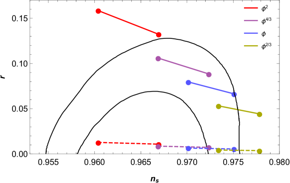
Figure 1: The $n_{s}$-$r$ points predicted by the model (72) for different parameters are confronted with Planck observation. The red, purple, blue and green lines correspond to the $\phi^{n}$ models with $n=2$, $n={4}/{3}$, $n=1$ and $n={2}/{3}$, respectively. The solid lines correspond to the $n_{s}$-$r$ values of the the models without $XR^{(3)}$. The dashed lines correspond to the shifted $n_{s}$-$r$ values in the corresponding models with the $XR^{(3)}$ coupling with $\beta=-0.60$. The dots on the left hand side and on the right hand side correspond to the e-folding number $N=50$ and $N=60$, respectively.

IV.2 Dilaton-like coupling coefficient

Now, we consider the case with a dilaton-like coupling coefficient

$$f_{1} = f_{0}e^{-\lambda\phi},~{}~{}~{}V=V_{0}\phi^{n}.$$ (78)

Similar to the previous model, one gets

$$f=\frac{1}{3}\beta n^{2}\phi^{n-2}e^{-\lambda\phi},~{}~{}~{}f_{\phi}=\frac{1}{3}\beta n^{2}\phi^{n-3}e^{-\lambda\phi}(n-2-\lambda\phi).$$ (79)

The Hubble flow parameter $\epsilon$ is same with the previous model, but

$$\eta=-\frac{1}{6}\beta n^{3}\phi^{n-4}e^{-\lambda\phi}(n-2-\lambda\phi).$$ (80)

The spectral index $n_{s}$ can be written as

$$n_{s}-1 = -n(n+2)\phi^{-2}+\frac{2\beta n\phi^{n-2}e^{-\lambda\phi}(n-\lambda\phi)}{1+\frac{4}{3}\beta\phi^{n}e^{-\lambda\phi}},$$ (81)

which involves model parameters $\beta$ and $\lambda$ in the slow-roll approximation.

We restrict ourselves to the $\phi^{2}$ model with $N=60$. The prediction of $n_{s}$-$r$ with the different values of the parameters $\beta$ and $\lambda$ is plotted in Fig.2. The green dot corresponds to $\beta=0$, which is the prediction of standard consistency relation without the coupling $XR^{(3)}$. From top to bottom, the red curves correspond to $\beta=-4\times 10^{-3},-8\times 10^{-3},-1.2\times 10^{-2},-1.6\times 10^{-2},-2.0\times 10^{-2}$, respectively.

In Fig.2, there exists parameter regions of $\beta$ and $\lambda$ where the predicted $n_{s}$-$r$ are consistent with the Planck constraints. It is noted that the predicted $r$ increases as $\lambda$ increases, but declines as $\beta$ increases. Compared with the power-law coupling discussed in previous section, the values of $n_{s}$-$r$ are actually more sensitive to the dilaton-like coupling. We can see that the negative coupling $\beta<0$ leads to a reduced tensor-to-scalar ratio, so that the $\phi^{2}$ model with $\beta<0$ can be driven to the $\sigma$ and $2\sigma$ contour, which is consistent with the observations very well.

Figure 2: The $n_{s}$-$r$ points predicted by the model (78) for different values of $\lambda$ and $\beta$ are confronted with Planck observation. Here we choose $N=60$. The green dot corresponds to the case with $\beta=0$, i.e., $\phi^{2}$ model without the $XR^{(3)}$ coupling.

IV.3 Constant coupling coefficient

For $\lambda=0$ in the previous subsection, the model reduces to a constant coupling case in which

$$f_{1} = f_{0},~{}~{}~{}V=V_{0}\phi^{n}.$$ (82)

One gets

$$f=\frac{1}{3}\beta n^{2}\phi^{n-2},~{}~{}~{}f_{\phi}=\frac{1}{3}\beta n^{2}\phi^{n-3}(n-2).$$ (83)

The Hubble flow parameter $\epsilon$ is same with the previous model, but

$$\eta=-\frac{1}{6}\beta n^{3}\phi^{n-4}(n-2).$$ (84)

The spectral index $n_{s}$ can be written as

$$n_{s}-1 = -n(n+2)\phi^{-2}+\frac{2\beta n^{2}\phi^{n-2}}{1+\frac{4}{3}\beta\phi^{n}},$$ (85)

which involves the model parameter $\beta$ in the slow-roll approximation.

For simplicity, we choose $N=60$. In Fig.3, we plot the $n_{s}$-$r$ predicted by the power law potentials $\phi^{n}$ with $n=2,4/3,1,2/3$. We can see that the corresponding $n_{s}$-$r$ values can be driven to the $\sigma$ and $2\sigma$ contours of Planck data in a suitable parameter range of $\beta$, which is consistent with the observations. However, contrary to the case in Fig.1, the $\phi^{n}$ potential with $n=4/3,1,2/3$ seems more favored than the potential with $n=2$.

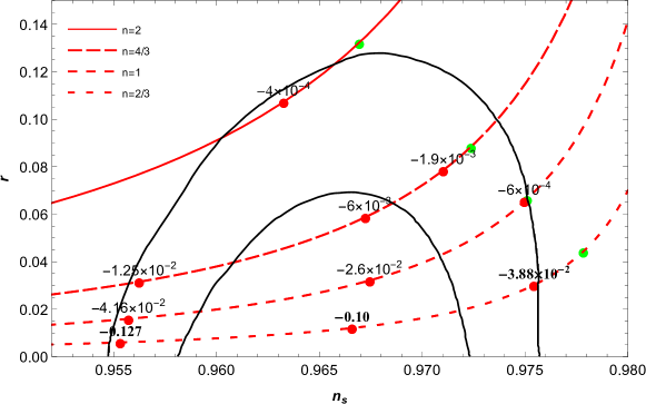
Figure 3: The $n_{s}$-$r$ points predicted by the model (82) with $n=2,4/3,1,2/3$ are confronted with Planck observation. Here we choose $N=60$. The red dots corresponds to the different non-zero values of $\beta$, and the green dots corresponds to the case with $\beta=0$, i.e.$\phi^{2}$ model without the $XR^{(3)}$ coupling.

V Conclusion

In this work, we have studied the slow-roll inflation with a non-minimally derivative coupling $XR^{(3)}$. We work in the frame in which the graviton behaves like in standard one, i.e. the propagating speed of gravitational waves equals to the speed of light, and analytically calculate the corrections of $XR^{(3)}$ on the power spectra of primordial perturbations. We plot the $n_{s}$-$r$ diagram for a few inflation models with the power-law coupling and the dilaton-like coupling, and find that the appearance of the $XR^{(3)}$ term can drives the $\phi^{2}$ inflation models to the best-fit region of the $n_{s}$-$r$ diagram.

Acknowledgments

YLH would like to thank Yong Cai and Gen Ye for helpful discussion. This work is supported by NSFC, Nos.11575188, 11690021, and also supported by the Strategic Priority Research Program of CAS, No.XDB23010100.

Appendix A the disformal transformation of covariant action

In this Appendix, we show that the covariant theory actually belongs to the beyond Horndeski theory and is preserved under certain disformal transformation.

Employing (6), the covariant action is

$$S = \int dx^{4}\sqrt{-g}\mathop{\Sigma}_{i}L_{i},$$ (86)

$$L_{2} = G_{2}(\phi,X),$$ (87)

$$L_{3} = G_{3}(\phi,X)\Box\phi,$$ (88)

$$L_{4} = G_{4}(\phi,X)R-2G_{4X}(\phi,X)\left(\Box\phi^{2}-\phi_{\mu\nu}\phi^{\mu\nu}\right),$$ (89)

$${}^{BH}{L}_{4} = F_{4}(\phi,\,X)\Big{[}X\left(\Box\phi^{2}-\phi_{\mu\nu}\phi^{\mu\nu}\right)-2\left(\Box\phi\,\phi_{\mu}\phi^{\mu\nu}\phi_{\nu}-\phi_{\mu}\phi^{\mu\nu}\phi_{\nu\rho}\phi^{\rho}\right)\Big{]},$$ (90)

with

$$G_{2} = -\frac{X}{2}-V-\frac{f_{1\phi\phi}}{2}X^{2},$$ (91)

$$G_{3} = -\frac{3}{2}f_{1\phi}X,$$ (92)

$$G_{4} = \frac{1}{2}(1+f_{1}X),$$ (93)

$$F_{4} = \frac{f_{1}}{2X}.$$ (94)

Here, we set $M_{p}=1$. Action (86) actually belongs to a subclass of the beyond Horndeski theory Gleyzes:2014qga ; Gleyzes:2014dya .

The disformal transformation of the metric (20) in covariant form reads

$$\tilde{g}_{\mu\nu}={C(\phi)}\left[g_{\mu\nu}-\left(1-\left(C(\phi)\right)^{2}\right)\frac{\phi_{\mu}\phi_{\nu}}{X}\right],$$ (95)

and the corresponding inverse transformation is

$$\tilde{g}^{\mu\nu}=\frac{1}{C(\phi)}\left[g^{\mu\nu}-\left(1-\left(C(\phi)\right)^{-2}\right)\frac{\phi^{\mu}\phi^{\nu}}{X}\right],$$ (96)

where $C(\phi)=\sqrt{1-f(\phi)},f(\phi)=f_{1}\dot{\phi}^{2}\left(t(\phi)\right)$, and $g_{\mu\nu}$ is identified as the metric in the original frame (86), while $\tilde{g}_{\mu\nu}$ is the metric in the new frame.

According to this transformation, we have

$$\tilde{S} = \int d\tilde{t}dx^{3}\sqrt{-\tilde{g}}\mathop{\Sigma}_{i}\tilde{L}_{i},$$ (97)

with the redefined coefficients

$$\tilde{G}_{2} = -\frac{\tilde{X}}{2}-C^{-3}V+\frac{3}{4}\alpha_{C}^{2}\tilde{X}-\frac{1}{2}\tilde{X}^{2}(f_{1}C)_{\phi\phi}$$ (99)

$$+\tilde{X}\left[(1+\alpha_{f})\left(\frac{\partial\alpha_{C}}{\partial\phi}-2\alpha_{C}^{2}\right)-\frac{1}{2}\frac{\partial\alpha_{C}}{\partial\phi}\right]\ln\tilde{X},$$

$$\tilde{G}_{3} = \alpha_{C}(\frac{1}{2}+\alpha_{f})\ln\tilde{X}+\alpha_{C}(1+2\alpha_{f})-\frac{3}{2}(f_{1}C)_{\phi}\tilde{X},$$ (100)

$$\tilde{G}_{4} = \frac{1}{2}C^{-2}+\frac{f_{1}}{2}C\tilde{X},$$ (101)

$$\tilde{F}_{4} = \frac{1}{2\tilde{X}^{2}}(f_{1}C\tilde{X}-\alpha_{f}).$$ (102)

The definitions of $\alpha_{f}$ and $\alpha_{C}$ are given in (25) and (40), respectively.

Apparently, this new action (97) maintains the same structure as (86), only up to a redefinition of the coefficients. Therefore, the disformal transformation (95) conserves the structure of (86) (see Gleyzes:2014qga for a discussion in the unitary gauge). Action (86) and action (97) both belong to a subset of the beyond Horndeski theory, and suffer from the restricted conditions

$$G_{5}(\phi,\tilde{X})=0,~{}~{}~{}F_{5}(\phi,\tilde{X})=0.$$ (103)

We can rewrite the covariant action as

$${\tilde{S}} = \int d\tilde{t}dx^{3}\sqrt{-\tilde{g}}\frac{1}{2}\Big{[}\tilde{R}+g(\phi,\tilde{X})\tilde{R}^{(3)}-\alpha_{C}\left(2+\ln\tilde{X}\right)\tilde{\Box}\phi$$ (104)

$$-\frac{\partial\alpha_{C}}{\partial\phi}\tilde{X}\ln\tilde{X}+\frac{3}{2}\alpha_{C}^{2}\tilde{X}-\tilde{X}-2C^{-3}V\Big{]},$$

with

$$g\tilde{R}^{(3)} = \left(\alpha_{f}+f_{1}C\tilde{X}\right)\tilde{R}+\frac{\alpha_{f}+f_{1}C\tilde{X}}{\tilde{X}}\left(\tilde{\phi}_{\mu\nu}\tilde{\phi}^{\mu\nu}-\Box\tilde{\phi}^{2}\right)$$ (105)

$$+2\frac{\alpha_{f}-f_{1}C\tilde{X}}{\tilde{X}^{2}}\left(\Box\tilde{\phi}\tilde{\phi}^{\mu}\tilde{\phi}_{\mu\nu}\tilde{\phi}^{\nu}-\tilde{\phi}^{\mu}\tilde{\phi}_{\mu\nu}\tilde{\phi}^{\nu\sigma}\tilde{\phi}_{\sigma}\right)$$

$$+2\left(-2\alpha_{C}C^{-2}\frac{1}{\tilde{X}}+(f_{1}C)_{\phi}\right)\left(\tilde{\phi}^{\mu}\tilde{\phi}_{\mu\nu}\tilde{\phi}^{\nu}-\tilde{X}\Box\tilde{\phi}\right),$$

$$g = \alpha_{f}+f_{1}C\tilde{X},$$ (106)

where $\tilde{\phi}_{\mu\nu}=\tilde{\nabla}_{\mu}\tilde{\nabla}_{\nu}\phi$, $\Box\tilde{\phi}=\tilde{g}^{\mu\nu}\tilde{\phi}_{\mu\nu}$. In unitary gauge, up to the second-order EFT operators, (104) is mapped to (24). By introducing the time-dependent parameter

$$\alpha=-\frac{C_{\phi}}{C}\dot{\phi},$$

which is equivalent to (18), and variation with respect to the metric and $\phi$, we obtain the background equations (27)-(29).

References

- (1) A. H. Guth, “The Inflationary Universe: A Possible Solution to the Horizon and Flatness Problems,” Phys. Rev. D 23, 347 (1981).
- (2) A. D. Linde, “A New Inflationary Universe Scenario: A Possible Solution of the Horizon, Flatness, Homogeneity, Isotropy and Primordial Monopole Problems,” Phys. Lett. 108B, 389 (1982).
- (3) A. Albrecht and P. J. Steinhardt, “Cosmology for Grand Unified Theories with Radiatively Induced Symmetry Breaking,” Phys. Rev. Lett. 48 (1982) 1220.
- (4) A. A. Starobinsky, “A New Type of Isotropic Cosmological Models Without Singularity,” Phys. Lett. B 91, 99 (1980) [Phys. Lett. 91B, 99 (1980)].
- (5) K. A. Malik and D. Wands, “Cosmological perturbations,” Phys. Rept. 475, 1 (2009) [arXiv:0809.4944 [astro-ph]].
- (6) D. H. Lyth and A. Riotto, “Particle physics models of inflation and the cosmological density perturbation,” Phys. Rept. 314, 1 (1999) [arxiv:hep-ph/9807278].
- (7) R. Kallosh and A. Linde, “Universality Class in Conformal Inflation,” JCAP 1307, 002 (2013) [arXiv:1306.5220 [hep-th]].
- (8) S. Ferrara, R. Kallosh, A. Linde and M. Porrati, “Minimal Supergravity Models of Inflation,” Phys. Rev. D 88, no. 8, 085038 (2013) [arXiv:1307.7696 [hep-th]].
- (9) M. Galante, R. Kallosh, A. Linde and D. Roest, “Unity of Cosmological Inflation Attractors,” Phys. Rev. Lett. 114, no. 14, 141302 (2015) [arXiv:1412.3797 [hep-th]].
- (10) L. Amendola, “Cosmology with nonminimal derivative couplings,” Phys. Lett. B 301, 175 (1993) [arXiv:[gr-qc/9302010]].
- (11) F. L. Bezrukov and M. Shaposhnikov, “The Standard Model Higgs boson as the inflaton,” Phys. Lett. B 659, 703 (2008) [arXiv:0710.3755 [hep-th]].
- (12) F. L. Bezrukov, A. Magnin and M. Shaposhnikov, “Standard Model Higgs boson mass from inflation,” Phys. Lett. B 675, 88 (2009) [arXiv:0812.4950 [hep-ph]].
- (13) A. De Simone, M. P. Hertzberg and F. Wilczek, “Running Inflation in the Standard Model,” Phys. Lett. B 678, 1 (2009) [arXiv:0812.4946 [hep-ph]].
- (14) F. Bezrukov and M. Shaposhnikov, “Standard Model Higgs boson mass from inflation: Two loop analysis,” JHEP 0907, 089 (2009) [arXiv:0904.1537 [hep-ph]].
- (15) F. Bezrukov, “The Higgs field as an inflaton,” Class. Quant. Grav. 30, 214001 (2013) [arXiv:1307.0708 [hep-ph]].
- (16) T. Markkanen, T. Tenkanen, V. Vaskonen and H. Veerm?e, “Quantum corrections to quartic inflation with a non-minimal coupling: metric vs. Palatini,” JCAP 1803, no. 03, 029 (2018) [arXiv:1712.04874 [gr-qc]].
- (17) C. Germani and A. Kehagias, “New Model of Inflation with Non-minimal Derivative Coupling of Standard Model Higgs Boson to Gravity,” Phys. Rev. Lett. 105 (2010) 011302 [arXiv:1003.2635 [hep-ph]].
- (18) C. Germani and A. Kehagias, “Cosmological Perturbations in the New Higgs Inflation,” JCAP 1005, 019 (2010) Erratum: [JCAP 1006, E01 (2010)] [arXiv:1003.4285 [astro-ph.CO]].
- (19) K. Feng, T. Qiu and Y. S. Piao, “Curvaton with nonminimal derivative coupling to gravity,” Phys. Lett. B 729, 99 (2014) [arXiv:1307.7864 [hep-th]].
- (20) K. Feng and T. Qiu, “Curvaton with nonminimal derivative coupling to gravity: Full perturbation analysis,” Phys. Rev. D 90, no. 12, 123508 (2014) [arXiv:1409.2949 [hep-th]].
- (21) Y. Huang, Y. Gong, D. Liang and Z. Yi, “Thermodynamics of scalar Ctensor theory with non-minimally derivative coupling,” Eur. Phys. J. C 75 (2015) no.7, 351 [arXiv:1504.01271 [gr-qc]].
- (22) N. Yang, Q. Fei, Q. Gao and Y. Gong, “Inflationary models with non-minimally derivative coupling,” Class. Quant. Grav. 33 (2016) no.20, 205001 [arXiv:1504.05839 [gr-qc]].
- (23) S. Capozziello, G. Lambiase and H. J. Schmidt, “Nonminimal derivative couplings and inflation in generalized theories of gravity,” Annalen Phys. 9 (2000) 39 [arXiv:gr-qc/9906051].
- (24) L. N. Granda, “Inflation driven by scalar field with non-minimal kinetic coupling with Higgs and quadratic potentials,” JCAP 1104, 016 (2011) [arXiv:1104.2253 [hep-th]].
- (25) R. Z. Ferreira, A. Notari and G. Simeon, “Natural Inflation with a periodic non-minimal coupling,” arXiv:1806.05511 [astro-ph.CO].
- (26) T. Tenkanen, “Resurrecting Quadratic Inflation with a non-minimal coupling to gravity,” JCAP 1712, no. 12, 001 (2017) [arXiv:1710.02758 [astro-ph.CO]].
- (27) K. Kaneta, O. Seto and R. Takahashi, “Very low scale Coleman-Weinberg inflation with nonminimal coupling,” Phys. Rev. D 97, no. 6, 063004 (2018) [arXiv:1708.06455 [hep-ph]].
- (28) S. Saichaemchan and B. Gumjudpai, “Non-minimal derivative coupling in Palatini cosmology: acceleration in chaotic inflation potential,” J. Phys. Conf. Ser. 901, no. 1, 012010 (2017) [arXiv:1703.09663 [gr-qc]].
- (29) N. Kaewkhao and B. Gumjudpai, “Cosmology of non-minimal derivative coupling to gravity in Palatini formalism and its chaotic inflation,” Phys. Dark Univ. 20, 20 (2018) [arXiv:1608.04014 [gr-qc]].
- (30) M. Artymowski, Z. Lalak and M. Lewicki, “Multi-phase induced inflation in theories with non-minimal coupling to gravity,” JCAP 1701, no. 01, 011 (2017) [arXiv:1607.01803 [astro-ph.CO]].
- (31) B. J. Broy, D. Coone and D. Roest, “Plateau Inflation from Random Non-Minimal Coupling,” JCAP 1606, no. 06, 036 (2016) [arXiv:1604.05326 [hep-th]].
- (32) H. Sheikhahmadi, E. N. Saridakis, A. Aghamohammadi and K. Saaidi, “Hamilton-Jacobi formalism for inflation with non-minimal derivative coupling,” JCAP 1610, no. 10, 021 (2016) [arXiv:1603.03883 [gr-qc]].
- (33) J. McDonald, “Nonminimally coupled inflation with initial conditions from a preinflation anamorphic contracting era,” Phys. Rev. D 94, no. 4, 043514 (2016) [arXiv:1511.07835 [astro-ph.CO]].
- (34) Y. Ema, R. Jinno, K. Mukaida and K. Nakayama, “Particle Production after Inflation with Non-minimal Derivative Coupling to Gravity,” JCAP 1510, no. 10, 020 (2015) [arXiv:1504.07119 [gr-qc]].
- (35) A. S. Arapoglu, “Generalized Slow-roll Inflation in Non-minimally Coupled Theories,” arXiv:1504.02192 [gr-qc].
- (36) S. del Campo, C. Gonzalez and R. Herrera, “Power law inflation with a non-minimally coupled scalar field in light of Planck 2015 data: the exact versus slow roll results,” Astrophys. Space Sci. 358, no. 2, 31 (2015) [arXiv:1501.05697 [gr-qc]].
- (37) T. Chiba and K. Kohri, “Consistency Relations for Large Field Inflation: Non-minimal Coupling,” PTEP 2015, no. 2, 023E01 (2015) [arXiv:1411.7104 [astro-ph.CO]].
- (38) H. Mohseni Sadjadi and P. Goodarzi, “Temperature in warm inflation in non minimal kinetic coupling model,” Eur. Phys. J. C 75, no. 10, 513 (2015) [arXiv:1409.5119 [gr-qc]].
- (39) B. Chen and Z. w. Jin, “Anisotropy in Inflation with Non-minimal Coupling,” JCAP 1409, no. 09, 046 (2014) [arXiv:1406.1874 [gr-qc]].
- (40) F. Darabi and A. Parsiya, “Cosmology with non-minimal coupled gravity: inflation and perturbation analysis,” Class. Quant. Grav. 32, no. 15, 155005 (2015) [arXiv:1312.1322 [gr-qc]].
- (41) H. Mohseni Sadjadi and P. Goodarzi, “Oscillatory inflation in non-minimal derivative coupling model,” Phys. Lett. B 732, 278 (2014) [arXiv:1309.2932 [astro-ph.CO]].
- (42) J. White, M. Minamitsuji and M. Sasaki, “Non-linear curvature perturbation in multi-field inflation models with non-minimal coupling,” JCAP 1309, 015 (2013) [arXiv:1306.6186 [astro-ph.CO]].
- (43) J. Kim, Y. Kim and S. C. Park, “Two-field inflation with non-minimal coupling,” Class. Quant. Grav. 31, 135004 (2014) [arXiv:1301.5472 [hep-ph]].
- (44) M. Artymowski, A. Dapor and T. Pawlowski, “Inflation from non-minimally coupled scalar field in loop quantum cosmology,” JCAP 1306, 010 (2013) [arXiv:1207.4353 [gr-qc]].
- (45) J. White, M. Minamitsuji and M. Sasaki, “Curvature perturbation in multi-field inflation with non-minimal coupling,” JCAP 1207, 039 (2012) [arXiv:1205.0656 [astro-ph.CO]].
- (46) Y. Cai, Y. Wan, H. G. Li, T. Qiu and Y. S. Piao, “The Effective Field Theory of nonsingular cosmology,” JHEP 1701, 090 (2017) [arXiv:1610.03400 [gr-qc]].
- (47) P. Creminelli, D. Pirtskhalava, L. Santoni and E. Trincherini, “Stability of Geodesically Complete Cosmologies,” JCAP 1611, no. 11, 047 (2016) [arXiv:1610.04207 [hep-th]].
- (48) Y. Cai, H. G. Li, T. Qiu and Y. S. Piao, “The Effective Field Theory of nonsingular cosmology: II,” Eur. Phys. J. C 77, no. 6, 369 (2017) [arXiv:1701.04330 [gr-qc]].
- (49) Y. Cai and Y. S. Piao, “A covariant Lagrangian for stable nonsingular bounce,” JHEP 1709, 027 (2017) [arXiv:1705.03401 [gr-qc]].
- (50) R. Kolevatov, S. Mironov, N. Sukhov and V. Volkova, “Cosmological bounce and Genesis beyond Horndeski,” JCAP 1708, no. 08, 038 (2017) [arXiv:1705.06626 [hep-th]].
- (51) J. Gleyzes, D. Langlois, F. Piazza and F. Vernizzi, “Exploring gravitational theories beyond Horndeski,” JCAP 1502, 018 (2015) [arXiv:1408.1952 [astro-ph.CO]].
- (52) J. Gleyzes, D. Langlois, F. Piazza and F. Vernizzi, “Healthy theories beyond Horndeski,” Phys. Rev. Lett. 114, no. 21, 211101 (2015) [arXiv:1404.6495 [hep-th]].
- (53) D. Langlois and K. Noui, “Degenerate higher derivative theories beyond Horndeski: evading the Ostrogradski instability,” JCAP 1602 (2016) no.02, 034 [arXiv:1510.06930 [gr-qc]].
- (54) P. Creminelli, J. Gleyzes, J. Nore?a and F. Vernizzi, “Resilience of the standard predictions for primordial tensor modes,” Phys. Rev. Lett. 113, no. 23, 231301 (2014) [arXiv:1407.8439 [astro-ph.CO]] .
- (55) S. Tsujikawa, “Disformal invariance of cosmological perturbations in a generalized class of Horndeski theories,” JCAP 1504, no. 04, 043 (2015) [arXiv:1412.6210 [hep-th]].
- (56) Y. Watanabe, A. Naruko and M. Sasaki, “Multi-disformal invariance of non-linear primordial perturbations,” EPL 111, no. 3, 39002 (2015) [arXiv:1504.00672 [gr-qc]].
- (57) G. Dom nech, A. Naruko and M. Sasaki, “Cosmological disformal invariance,” JCAP 1510, no. 10, 067 (2015) [arXiv:1505.00174 [gr-qc]].
- (58) C. Cheung, P. Creminelli, A. L. Fitzpatrick, J. Kaplan and L. Senatore, “The Effective Field Theory of Inflation,” JHEP 0803 (2008) 014 arXiv:0709.0293 [hep-th].
- (59) L. Bordin, G. Cabass, P. Creminelli and F. Vernizzi, “Simplifying the EFT of Inflation: generalized disformal transformations and redundant couplings,” JCAP 1709, no. 09, 043 (2017) [arXiv:1706.03758 [astro-ph.CO]].
- (60) Y. Cai, Y. T. Wang and Y. S. Piao, “Is there an effect of a nontrivial during inflation?,” Phys. Rev. D 93, no. 6, 063005 (2016) [arXiv:1510.08716 [astro-ph.CO]].
- (61) Y. Cai, Y. T. Wang and Y. S. Piao, “Propagating speed of primordial gravitational waves and inflation,” Phys. Rev. D 94, no. 4, 043002 (2016) [arXiv:1602.05431 [astro-ph.CO]].
- (62) D. J. Schwarz, C. A. Terrero-Escalante and A. A. Garcia, “Higher order corrections to primordial spectra from cosmological inflation,” Phys. Lett. B 517, 243 (2001) [astro-ph/0106020].
- (63) S. M. Leach, A. R. Liddle, J. Martin and D. J. Schwarz, “Cosmological parameter estimation and the inflationary cosmology,” Phys. Rev. D 66, 023515 (2002) [astro-ph/0202094].
- (64) A. De Felice and S. Tsujikawa, “Inflationary gravitational waves in the effective field theory of modified gravity,” Phys. Rev. D 91, no. 10, 103506 (2015) [arXiv:1411.0736 [hep-th]].