The Entropy of Cantor–like measures

Abstract.

By a Cantor-like measure we mean the unique self-similar probability measure $\mu$ satisfying $\mu=\sum_{i=0}^{m-1}p_{i}\mu\circ S_{i}^{-1}$ where $S_{i}(x)=\frac{x}{d}+\frac{i}{d}\cdot\frac{d-1}{m-1}$ for integers $2\leq d<m\leq 2d-1$ and probabilities $p_{i}>0$, $\sum p_{i}=1$. In the uniform case ($p_{i}=1/m$ for all $i$) we show how one can compute the entropy and Hausdorff dimension to arbitrary precision. In the non-uniform case we find bounds on the entropy.

1. Introduction

By a self-similar measure we mean the unique probability measure

$$\mu=\sum_{i=0}^{m-1}p_{i}\mu\circ S_{i}^{-1},$$

where $S_{i}$ are linear contractions on $\mathbb{R}$ and $p_{i}>0$ are probabilities with $\sum_{i=0}^{m-1}p_{i}=1$. We restrict our attention to those measures whose support is $[0,1]$. It is known that these self-similar measures are either purely singular or absolutely continuous with respect to Lebesgue measure [15], but it is often difficult to determine which is the case for a particular example.

An interesting class of examples are the Bernoulli convolutions where $m=2$, $S_{0}(x)=x/\varrho$ and $S_{1}=x/\varrho+1-1/\varrho$ for some $\varrho\in(1,2)$. These have been extensively studied since the 1930’s when Erdös [7] showed that if $\varrho\in(1,2)$ was a Pisot number, then the Bernoulli convolution was purely singular and later, in [8], that the Bernoulli convolutions were absolutely continuous for almost all $\varrho\in(1,2)$. For more on the history of these classical problems see [19, 21].

In [11], Garsia showed that the notion of entropy was useful for studying the dimensional properties of Bernoulli convolutions. Subsequently, the Garsia entropy was computed for various Bernoulli convolutions, first for $\varrho=(1+\sqrt{5})/2$, the golden ratio (a simple Pisot number) in [2], then for all simple Pisot numbers in [3, 12], and, finally, for all algebraic integers in [1, 4]. Edson, in [6], generalized these results in a different direction, considering the contraction factor $1/\varrho$ where $\varrho$ is the root of $x^{2}-ax-b$ with $a\geq b$ and $a$ equally spaced linear contractions.

This paper focuses on a different generalization, to the case where $\varrho=d$ is an integer greater than or equal to $2$ and $m$ equally spaced contractions $S_{j}$ of the form

(1.1) $$S_{j}(x)=\frac{x}{d}+\frac{j}{d}\cdot\frac{d-1}{m-1}\hskip 28.45274ptj=0,1,\dots,m-1$$

where $2\leq d<m\leq 2d-1$. If, for example, $d=3$, $m=4$ and the probabilities satisfy $p_{0}=p_{3}=1/8$, $p_{1}=p_{2}=3/8$, then the associated self-similar measure is the $3$-fold convolution product of the classical middle-third Cantor measure. We call these self-similar Cantor-like measures, $(m,d)$-measures, and refer to them as uniform if all $p_{i}$ are equal. The dimensional properties of these measures are also of much interest; see, for example, [5, 13, 17, 20].

We use combinatorial techniques to find an (explicit) analytic function $T$ with the property that the Garsia entropy of the uniform $(m,d)$-measure is given by $T(1)/\log_{2}d$ when $2\leq d<m\leq 2d-1$. This is done in Section 3 where we first illustrate the method with the simple case $d=2,$ $m=3$, and then handle the general uniform $(m,d)$-measure. Bounds are found for the Garsia entropy of the non-uniform $(m,d)$-measures, a more complicated problem, in Section 4. In Section 5, we use precise information about the function $T$ to give numerically significant estimates for the entropy in the uniform case when $2\leq d\leq 10$ and give ranges for the value of the entropy for some non-uniform examples. We begin, in Section 2, with the definition of the Garsia entropy and a discussion of some of the combinatorial ideas we use in the proofs.

As with sets, there is a notion of the Hausdorff dimension of a probability measure $\mu$ defined as

$$\dim_{H}\mu=\inf\{\dim_{H}E:\mu(E)>0\}.$$

If $\mu$ is a measure on $\mathbb{R}$ and $\dim_{H}\mu<1,$ then $\mu$ is singular. For self-similar measures arising from a set of contractions that satisfy the open set condition there is a simple formula for computing $\dim_{H}\mu$ (c.f. [9]). But neither the Bernoulli convolutions nor the Cantor–like measures satisfy this separation property and their Hausdorff dimensions can be difficult to compute. It is a deep result of Hochman [14] (see [4] for details) that the Hausdorff dimension of measures on $\mathbb{R}$ satisfying a suitable separation condition (which includes Bernoulli convolutions with contraction factor an algebraic number and the $(m,d)$-measures) is the minimum of $1$ and the Garsia entropy of the measure, thus our results also give new estimates on the Hausdorff dimensions of these measures.

The Hausdorff dimension of a self-similar measure can also be found from its $L^{q}$ spectrum; see [18] for details. Using this approach, infinite series representations have been found in [16] for the Hausdorff dimension of the $(d,d+1)$-measures and in [10] for Bernoulli convolutions with contraction factor the inverse of a of simple Pisot number. These involve matrix products, hence are less computationally efficient. Numerical values (to four digits) were given in [16] for the special case of the $3$-fold convolution of the classic Cantor measure.

2. A combinatorial approach to the Garsia entropy

2.1. The $(m,d)$-graph and entropy of the $(m,d)$-measure

We will take a combinatorial approach to studying the Garsia entropy of the Cantor-like $(m,d)$-measures $\mu=\sum_{j=0}^{m-1}p_{j}\mu\circ S_{j}^{-1},$ with $S_{j}$ as in (1.1) and integers $d,m$ satisfying $2\leq d<m\leq 2d-1$.

For this, we will need to introduce further notation. Given $\sigma\in\{0,1,\dots,m-1\}^{n}$, say $\sigma=(\sigma_{1},\sigma_{2},\dots,\sigma_{n}),$ we set $S_{\sigma}=S_{\sigma_{1}}\circ\dots\circ S_{\sigma_{n}}$ and call $\sigma$ a word of length $\left|\sigma\right|=n$. We write $p_{\sigma}$ for the product $p_{\sigma_{1}}\cdot\cdot\cdot p_{\sigma_{n}}$.

It is possible for $S_{\sigma}=S_{\tau}$ with $\left|\sigma\right|=\left|\tau\right|$, but $\sigma\neq\tau$; the Garsia entropy takes into account how often these overlaps occur and the associated probabilities. To compute this, we create a graph where there is a single root, which we can think of as $S_{\emptyset}(0)$. The nodes at level $n\geq 1$ are the distinct images $S_{\sigma}(0)$ for $|\sigma|=n$ and a node $S_{\sigma}(0)$ at level $n$ is connected to all the nodes of the form $S_{\sigma i}(0)$, $i=0,1,\dots,m-1$ at level $n+1$. We call this the $(m,d)$-graph. See Figure 1 for an example.

Denote by $g_{n}$ the set of nodes at level $n\geq 0$ in the graph. For $z\in g_{n}$, we will denote by $[z]_{n}$ the set of all $\sigma$ with $\left|\sigma\right|=n$ such that $z=$ $S_{\sigma}(0)$. We assign weight $w_{z}$ to the node $z$, where

$$w_{z}=\sum_{\sigma\in[z]_{n}}p_{\sigma}$$

and we let $W_{n}$ denote the set of all weights $w_{z}$ associated to some $z\in g_{n}$.

The entropy of the $n$^th level of the weighted $(m,d)$-graph associated with the $(m,d)$-measure $\mu$ is defined as

(2.1) $$h_{\mu}(n)=-\sum_{w_{z}\in W_{n}}w_{z}\log_{2}w_{z}$$

and the Garsia entropy $\mathfrak{H}_{\mu}$ (hereafter called the entropy) of $\mu$ is given by

(2.2) $$\mathfrak{H}_{\mu}=\lim_{n\rightarrow\infty}\frac{h_{\mu}(n)}{n\log_{2}d}.$$

Another way to describe this calculation is as follows. Put

$$\mu_{n}=\bigotimes{}_{k=1}^{n}\left(\sum_{j=1}^{n}p_{j}\delta_{\frac{j(d-1)}{m-1}d^{-k}}\right)$$

where $\bigotimes$ denotes the convolution product. These discrete measures converge weak $\ast$ to $\mu$ and supp$\mu_{n}=\{S_{\sigma}(0):\left|\sigma\right|=n\}$. Denote by $D_{n}$ the partition of $[0,1]$ into $(m-1)d^{n}$ equally spaced points. Each subinterval $[a,b)$ of $D_{n}$ can be identified with a unique node at level $n$, namely the node $z$ such that $S_{\sigma}(0)$ belongs to the subinterval for $\sigma\in[z]_{n}$. The weight, $w_{z}$, equals $\mu_{n}([a,b))$.

With this notation, we have

$$h_{\mu}(n)=-\sum_{\Delta\in D_{n}}\mu_{n}(\Delta)\log_{2}(\mu_{n}(\Delta)).$$

Thus one can see that $h_{\mu}(n)=H(\mu_{n},D_{n})$ (where $D_{n}$ is the partition we have described, rather than the partition into $2^{n}$ equally spaced points), in the notation of [14].

In the case of the uniform $(m,d)$-measure, the measure $\mu,$ and hence also $h_{\mu}$ and $\mathfrak{H}_{\mu},$ depend only on $m$ and $d$, and we will write $h_{m,d}$ and $\mathfrak{H}_{m,d}$. The entropy calculation can be simplified in this case: We will let $\mathrm{freq}(z)$ denote the number of paths from the root node to $z\in g_{n}$. As $p_{\sigma}=m^{-n}$ for all $\sigma$ of length $n$, $w_{z}=m^{-n}\mathrm{freq}(z)$. Thus

(2.3) $$h_{m,d}(n)=-\sum_{z\in g_{n}}(m^{-n}\mathrm{freq}(z))\log_{2}(m^{-n}\mathrm{freq}(z)).$$

If we let $f_{m,d}(n,k)$ denote the number of nodes in level $n$ with frequency $k,$ then we have

$$h_{m,d}(n) = \sum_{k=1}^{\infty}\sum_{\begin{subarray}{c}z\in g_{n},\\ \mathrm{freq}(z)=k\end{subarray}}m^{-n}k\log_{2}(m^{-n}k)$$

$$= -m^{-n}\sum_{k=1}^{\infty}f_{m,d}(n,k)k(-n\log_{2}m+\log_{2}k).$$

Since the total number of nodes at level $n$ (counted by frequency) is $m^{n},$ this reduces to

(2.4) $$h_{m,d}(n)=n\log_{2}m-m^{-n}\sum_{k=1}^{\infty}f_{m,d}(n,k)k\log_{2}k.$$

When $\mu,m$ or $d$ are clear, we may suppress them in the notation.

2.2. Generating functions associated with the $(m,d)$ graph

For studying the entropy of the uniform $(m,d)$-measure it is helpful to introduce generating functions associated with the $(m,d)$-graph: Denote by

$$H(x)=H_{m,d}(x)=\sum_{n=0}^{\infty}h_{m,d}(n)x^{n}$$

the generating function for the entropies of the levels of the $(m,d)$-graph and denote by $F_{k}$ the generating function (for the number of nodes of frequency $k$ at each level) of the $(m,d)$-graph,

$$F_{k}(x)=\sum_{n=0}^{\infty}f(n,k)x^{n},$$

and the related function

$$\mathcal{F}(x,s)=\sum_{k=2}^{\infty}k^{s}F_{k}(x).$$

Since we assume $m\leq 2d-1$, the largest frequency at level $n$ is at most twice the largest frequency at level $n-1$ and thus $f(n,k)=0$ if $k>2^{n}$. Further, $f(n,k)\leq m^{n}$, hence $F_{k}(x)=\sum_{n\geq\log_{2}k}f(n,k)x^{n}$ and

$$\left|F_{k}(x)\right|\leq\sum_{n\geq\log_{2}k}m^{n}\left|x\right|^{n}\leq c\varepsilon^{\log_{2}k}\text{ if }\left|x\right|\leq\varepsilon/m.$$

It follows from these bounds that for $x$ small enough, $\frac{\partial}{\partial s}\mathcal{F}(x,s)|_{s=1}$ can be obtained by differentiating the series term-by-term.

2.3. Euclidean tree

The $(m,d)$-graph is closely connected to the Euclidean tree, as we will explain in Sections 3.1 and 3.2, and will be helpful in studying the entropy of the uniform $(m,d)$-measure. Here we describe the construction of the Euclidean tree.

Start with two nodes connected by an edge, a root node with label $\{1,1\}$ at level $n=0$ and a node with label $\{2,1\}$ at level $n=1$. For each node $\{a,b\}$ in level $n\geq 1$, add two children with labels $\{a,a+b\}$ and $\{a+b,b\}$ in level $n+1$. This graph is the Euclidean tree and is illustrated in Figure 3.

Notice that all labels in the Euclidean tree are coprime pairs and that a path from some node $\{a,b\}$ in the Euclidean tree to the root records the steps involved in executing the simple Euclidean algorithm (the Euclidean algorithm, but with repeated subtraction replacing division) on the pair $\{a,b\}$. Define $e(k,i)$ to be the number of steps it takes to reduce the pair $\{k,i\}$ to their GCD via the simple Euclidean algorithm. For every coprime pair $\{k,i\}$, $e(k,i)=n$ if and only if the pair $\{k,i\}$ is found on level $n$ of the Euclidean tree. We refer the reader to [2] for further description and the history of the Euclidean tree.

Let $a(n,k)$ be the number of times that the integer $k$ occurs as the larger value of a label at level $n$ of the Euclidean tree and let

$$A_{k}(x)=\sum_{n=0}^{\infty}a(n,k)x^{n}=\sum_{\begin{subarray}{c}1\leq i\leq k\\ \gcd(i,k)=1\end{subarray}}x^{e(k,i)}$$

be the generating function (for occurrences of $k$ in level $n)$ of the Euclidean tree. (In our notation, $A_{k}(x)$ is the function $\hat{\alpha}(x)$ in [2].) Each occurrence of $k\geq 2$ as a label (larger or smaller) in the Euclidean tree can be traced up the Euclidean tree to an occurrence as the larger label, and each time $k$ appears as a larger label there is a single line of descendants in which it appears as the smaller label. For instance, the 2 in the label $\{5,2\}$ on level $n=3$ of the Euclidean tree can be traced back up to the label $\{1,2\}$ on level 1. Thus, the family of generating functions for larger and smaller labels in the Euclidean tree is $(1+x+x^{2}+\ldots)A_{k}(x)=\frac{1}{1-x}A_{k}(x)$ for $k\geq 2$.

We define

$$\mathcal{A}(x,s)=\sum_{k=2}^{\infty}k^{s}A_{k}(x)=\sum_{n}x^{n}\sum_{\begin{subarray}{c}1\leq i\leq k\\ \gcd(i,k)=1\\ e(k,i)=n\end{subarray}}k^{s}$$

and, as with $\mathcal{F(}s,x),$ one can show that $\frac{\partial}{\partial s}\mathcal{A}(x,s)|_{s=1}$ can be obtained by differentiating the series term-by-term for sufficiently small $x$.

3. Entropy of the uniform $(m,d)$-measures

3.1. The entropy generating function for the $d=2,m=3$ case

In this first subsection we consider the case when $d=2$ and $m=3$. This case will illustrate the key combinatorial ideas without the complications that arise in the general case, making precise the relationship between $F_{k}(x)$ (the generating function of the $(m,d)$-graph), $A_{k}(x)$ (the generating function for the Euclidean tree), and $H_{k}(x)$ (the entropy generating function).

Figure 1 shows the first few levels of the $(3,2)$-graph associated with the $(3,2)$-measure. Each node has three children: a middle child, whose frequency is the same as its parent, and a left and a right child. The left child of a node $X$ is the right child of $X$’s left neighbour, and thus its frequency is the sum of those of its parents. The analogous situation holds for the right child. A node of frequency $k$ induces a column of frequency-$k$ nodes below it.

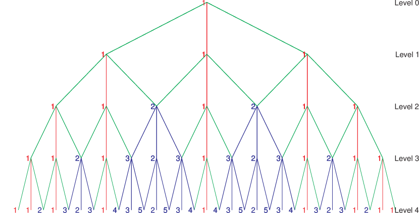
Figure 1. The infinite self-similar graph associated with the $(3,2)$-measure

3.1.1. Generating functions of subgraphs

The first step is to partition the full $(3,2)$-graph into subgraphs we call the $G$ and $P$-subgraphs. We will show that the $G$-subgraph is closely related to the Euclidean tree and using this we will see how to compute its generating functions. The $P$-subgraphs turn out to be very simple in this particular case.

Note that the only frequency-one nodes in the graph are on the left and right arcs descending from the top node and in the columns below the nodes in those arcs. It is easy to see that these columns of ones partition the graph into an infinite number of copies of the subgraph depicted in Figure 2, with two copies starting at each level. We will call the subgraphs between these column of ones the G-subgraphs. Note, for example, that there are no nodes of the $G$-subgraph at relative level 0, one node of weight 2 at level 1 and three nodes (two of weight 3 and one of weight 2) at level 2.

We will let $G_{k}(x)$ be the generating function for the number of nodes of weight $k$ at level $n$ of the $G$-subgraph. For example $G_{5}(x)=2x^{3}+4x^{4}+\dots$.

The column of ones that divide various $G$-subgraphs will be called the P-subgraphs. The generating functions for the $P$-subgraphs are simply

$$P_{1}(x)=1+x+x^{2}+\cdots=\frac{1}{1-x}\text{ and }P_{k}(x)=0\text{ for }k\geq 2.$$

There is one $P$-subgraph starting at level 0 and two $P$-subgraphs starting at each level $n\geq 1$. In addition, there are two $G$-subgraphs starting at level $n$ for all $n\geq 1$. This gives the relationship

(3.1) $$F_{k}(x)=P_{k}(x)+\frac{2x}{1-x}P_{k}(x)+\frac{2x}{1-x}G_{k}(x).$$

Figure 2. The $G$-subgraph (blue) and $P$-subgraphs (red) bounding it

The $G$-subgraph essentially consists of two copies of the dual graph of the Euclidean tree, as we now explain. Note that the $G$-subgraph is symmetric about the middle column of twos. If we take the dual graph of one of its halves, and label each resulting node with the pair of nodes adjacent to it in the $G$-subgraph (see Figure 3), then we get the Euclidean tree. Figure 3 gives the first few levels of the Euclidean tree, as well as demonstrating its duality with the $G$-subgraph.

Figure 3. The $G$-subgraph (blue) and $P$-subgraphs (red) bounding it and the Euclidean tree dual (black)

Since the generating functions for larger and smaller labels in the Euclidean tree is given by $\frac{1}{1-x}A_{k}(x)$ for $k\geq 2$, as explained in the previous section, the duality relationship between the Euclidean tree and the $G$-subgraph implies that the generating function for the $G$-subgraph is

$$G_{1}(x)=0\text{, }G_{k}(x)=\frac{1}{1-x}A_{k}(x)\text{ for }k\geq 2\text{.}$$

Combining this with equation (3.1) shows that for $k\geq 2$,

(3.2) $$F_{k}(x)=P_{k}(x)+\frac{2x}{1-x}P_{k}(x)+\frac{2x}{(1-x)^{2}}A_{k}(x)=\frac{2x}{(1-x)^{2}}A_{k}(x).$$

3.1.2. The analytic extension of the entropy generating function

Theorem 3.1.

Let $H_{3,2}(x)=\sum_{n=1}^{\infty}h_{3,2}(n)x^{n}$ be the generating function for the entropies of the levels of the $(3,2)$-graph. There exists a function $T_{3,2}(x)$, analytic on a disk of radius $3$ about $0$, such that

$$H_{3,2}(x)=\frac{x}{(x-1)^{2}}T_{3,2}(x).$$

Corollary 3.2.

With $T_{3,2}(x)$ defined as above, we have

$$\mathfrak{H}_{3,2}=T_{3,2}(1).$$

Proof.

Let $U=\{x:|x|<3\}$. As $T(x)=T_{3,2}(x)$ is analytic on $U$, we see that $H(x)=H_{3,2}(x)$ is analytic on $U\setminus\{1\}$. As $H(x)=\frac{x}{(x-1)^{2}}T(x)$ and $T(x)$ is analytic on a disk of radius 2 around $1$, there must exist coefficients $c(n)$ and $d(n)$ such that

$$H(x) =\sum_{n=0}^{\infty}h(n)x^{n}=x\sum_{n=-2}^{\infty}c(n)(x-1)^{n}$$

$$=x\left(\frac{T(1)}{(x-1)^{2}}+\frac{T^{\prime}(1)}{x-1}+\sum_{n=0}^{\infty}c(n)(x-1)^{n}\right)$$

$$=x\left(\frac{T(1)}{(x-1)^{2}}+\frac{T^{\prime}(1)}{x-1}+\sum_{n=0}^{\infty}d(n)x^{n}\right)$$

Since $H(x)$ is analytic on $U\setminus\{1\},$ we see that $\sum_{n=0}^{\infty}d(n)x^{n}$ is analytic on $U$ and hence $d(n)\rightarrow 0$ as $n\rightarrow\infty$. Further, $h(n)=T(1)n-T^{\prime}(1)+d(n-1)$, whence

$$\mathfrak{H}_{3,2}=\lim_{n\rightarrow\infty}\frac{h(n)}{n\log_{2}2}=T(1).$$

∎

Proof of Theorem 3.1.

We remind the reader that $\mathcal{A}(x,s)=\sum_{k=2}^{\infty}k^{s}A_{k}(x)$ and $\mathcal{F}(x,s)=\sum_{k=2}^{\infty}k^{s}F_{k}(x)$. As these sums begin with $k=2$ and $P_{k}=0$ for $k\geq 2$, equation (3.2) shows

(3.3) $$\mathcal{F}(x,s)=\frac{2x}{(1-x)^{2}}\mathcal{A}(x,s),$$

while differentiating the series $\sum k^{s}F_{k}(x)$ term-by-term with respect to $s$ gives

$$\frac{\partial}{\partial s}F(x,s) = \sum_{k}k^{s}\ln kF_{k}(x)$$

$$= \sum_{k}k^{s}\ln k\sum_{n}f(n,k)x^{n}.$$

From (2.4), we have

$$h(n)=n\log_{2}3-3^{-n}\sum_{k=1}^{\infty}f(n,k)k\log_{2}k,$$

thus

$$H(x) =\sum_{n=0}^{\infty}h(n)x^{n}=\sum_{n=0}^{\infty}\left(n\log_{2}3-3^{-n}\sum_{k=1}^{\infty}f(n,k)k\log_{2}k\right)x^{n}$$

$$=\sum_{n=0}^{\infty}nx^{n}\log_{2}3-\frac{1}{\ln 2}\left.\frac{\partial}{\partial s}\mathcal{F}(x/3,s)\right|_{s=1}$$

$$=\frac{x}{(1-x)^{2}}\log_{2}3-\frac{2x}{3(1-x/3)^{2}\ln 2}\left.\frac{\partial}{\partial s}\mathcal{A}(x/3,s)\right|_{s=1}$$

where the final equality simply follows from (3.3). Differentiating the series $\sum_{k}k^{s}A_{k}(x)$, simplifying and using the definition of $A_{k}$ yields

$$H(x) =\frac{x}{(1-x)^{2}}\log_{2}3-\frac{2x}{3(1-x/3)^{2}}\sum_{k=2}^{\infty}k\log_{2}kA_{k}\left(\frac{x}{3}\right)$$

$$=\frac{x}{(1-x)^{2}}\left(\log_{2}3-\frac{2(1-x)^{2}}{3(1-x/3)^{2}}\sum_{k=2}^{\infty}k\log_{2}kA_{k}\left(\frac{x}{3}\right)\right)$$

$$=\frac{x}{(1-x)^{2}}\left(\log_{2}3-\frac{2(1-x)^{2}}{3(1-x/3)^{2}}\sum_{n=1}^{\infty}\left(\frac{x}{3}\right)^{n}\sum_{\begin{subarray}{c}k>i,\gcd(i,k)=1\\ e(k,i)=n\end{subarray}}k\log_{2}k\right).$$

Finally, putting

$$L(x)=\sum_{n=1}^{\infty}\ell(n)x^{n}=(1-3x)^{2}\sum_{n=1}^{\infty}x^{n}\sum_{\begin{subarray}{c}k>i,\gcd(i,k)=1\\ e(k,i)=n\end{subarray}}k\log_{2}k,$$

we conclude that

$$H(x)=\frac{x}{(1-x)^{2}}\left(\log_{2}3-\frac{2}{3(1-x/3)^{2}}L(x/3)\right).$$

By [12], if $L(x)=\sum_{n=1}^{\infty}\ell(n)x^{n}$, then for $n\geq 3$, $|\ell(n)|\leq\frac{2}{15\ln 2}$. This implies that $\sum_{n=1}^{\infty}\ell(n)x^{n}$ converges on the unit disk in the complex plane, hence $H(x)$ has an analytic continuation to all $|x|<3$, as required. Letting

$$T(x)=\log_{2}3-\frac{2}{3(1-x/3)^{2}}L(x/3)$$

gives the desired result. ∎

3.2. The entropy generating functions for the general uniform $(m,d)$-measure

3.2.1. Generating functions of related subgraphs in the general case

In the previous subsection, we used the fact that the $(3,2)$-graph can be partitioned into a number of $G$-subgraphs and $P$-subgraphs and then showed how the $G$-subgraph was related to the Euclidean tree. That allowed us to find a generating function for the number of nodes of weight $k$ at level $n$ for the $(3,2)$-graph from which we developed the generating function for the entropy.

In this subsection we will extend the notions of the $G$-subgraphs and $P$-subgraphs to the more general set up. Unfortunately, the $P$-subgraphs are no longer simple as they will contain nodes with weights higher than 1. Both graphs are still related to the Euclidean tree however, thus allowing us to derive relations of $H(x)$ as before.

Figure 4. The infinite self-similar graph associated with the $(4,3)$-measure

Figure 5. The infinite self-similar graph associated with the $(5,3)$-measure

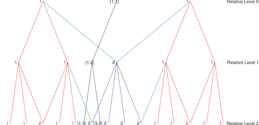
Figure 6. The $G$-subgraph (blue) and $P$-subgraphs (red) bounding it and the Euclidean graph dual (black)

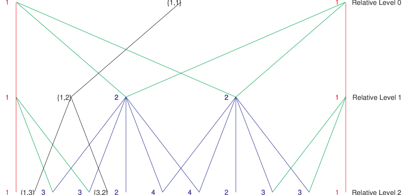
Figure 7. The $G$-subgraph (blue) and $P$-subgraphs (red) bounding it and the Euclidean graph dual (black)

Figures 4 and 5 show the structure of the $(4,3)$ and $(5,3)$-graphs. For a general $(m,d)$-graph, each node has $m$ children, and in general (assuming the parent has a neighbour on each side), the leftmost and rightmost $r=m-d$ children will be “overlapping” and have a second parent, the first parent’s left or right neighbour. This is because $S_{i,j+d}=S_{i+1,j}$ for $j=0,\dots,r-1$ and otherwise, $S_{i,k}\neq S_{\ell,j}$ since $m\leq 2d-1$. This leaves $d-r$ non-overlapping children in the middle. The fact that two nodes on the same level share a descendent if and only if they are adjacent is the fundamental property that permits our analysis to work.

As before, we will partition the $(m,d)$-graph into $P$-subgraphs and $G$-subgraphs, but the definition of these two subgraphs will need to be modified for this more general case. The $P$-subgraph will begin with a single node of weight $1$ at (relative) level 0. In the $(m,d)$-graph, this node has $m=d+r$ children. We include in this $P$-subgraph all children of this node, except the outer $r$ children on the left and on the right. These inner, first level, children will always have weight $1$ (regardless of the level of the original graph at which they begin). At the next level, we consider again all children of these $d-r$ nodes, except the outer most $r$ right children of the right most node, and the outer most $r$ left children of the left most node. Note that some of these children will have weight greater than $1$. We repeat this process for each lower level with new $P$-subgraphs beginning on each level on these previously excluded outer most nodes. We see that the outer most children of the $P$-subgraph have weight $1$. Examples of $P$-subgraphs are given with red nodes in Figures 4 and 5. Notice that if $m=2d-1$ ($r=d-1)$, the $P$-subgraph is a single column of ones, as in the previous section.

We define the $G$-subgraph to consist of the nodes between two adjacent $P$-subgraphs (not necessarily arising on the same level). As before, the $G$-subgraph has no nodes at relative (to the $P$-subgraphs) level 0. It will have $r$ nodes at relative level $1$ of weight $2$. Examples of $G$-subgraphs are given with blue nodes in Figures 4 and 5.

The generating function, $F_{k},$ of nodes of weight $k$ at level $n$ for the $(m,d)$-graph, can again be written in terms of the generating functions of the $G$-subgraphs and $P$-subgraphs. Indeed, we see that there is a single $P$-subgraph starting at level $0$, $2r$ $P$-subgraphs starting at level $1$ and, more generally, there are $2r$ $P$-subgraphs starting at every level $n\geq 1$. Between each of pair of $P$-subgraphs there is a $G$-subgraph. Thus there are $2r$ $G$-subgraphs starting at every level $n\geq 1$. This gives us the relationship

(3.4) $$F_{k}(x)=P_{k}(x)+\frac{2rx}{1-x}P_{k}(x)+\frac{2rx}{1-x}G_{k}(x)$$

(which, of course, coincides with (3.1) in the case $d=2$, $m=3$).

Having defined the $P$ and $G$-subgraphs, we now determine their generating functions. First, consider a $P$-subgraph in the special case $r=d-1$. Then the generating function is the same as before, namely $P_{1}(x)=\frac{1}{1-x}$, $P_{k}(x)=0$ for $k\geq 2$.

If $r\neq d-1$, then the generating function is more complicated. The $P$-subgraph has a single node of weight $1$ at level $0$ and $d-r$ children at level $1$ of weight $1$. These children can also be viewed as the starting node of their own $P$-subgraph. Between each of these $d-r$ children there is a $G$-subgraph. This gives us the relations

$$P_{1}(x) =1+(d-r)xP_{1}(x),$$

$$P_{k}(x) =(d-r)xP_{k}(x)+(d-r-1)xG_{k}(x)\text{ for }k\geq 2.$$

Note these coincide with the equations given above in the special case $r=d-1$ and simplify to

(3.5) $$P_{1}(x)=\frac{1}{1-(d-r)x},\text{ }P_{k}(x)=\frac{(d-r-1)x}{1-(d-r)x}G_{k}(x)\text{ for }k\geq 2.$$

Now, consider the $G$-subgraph. As before, there is a relationship between the $G$-subgraph and the Euclidean graph. To be more precise, there is a relationship between the generating function for $G_{k}(x)$ and for $A_{k}(x)$. Consider a node in the Euclidean graph $\{a,b\}$ at level $n$ with children $\{a,a+b\}$ and $\{a+b,b\}$ at level $n+1$. Between these two children there are $r$ nodes of weight $a+b$. Each of these nodes can be thought of as the top node of an $(a+b)$ multiple of a $P$-subgraph. In particular this means that the number of nodes of weight $k$ in one of these $(a+b)$ multiples of a $P$-subgraph is the same as the number of weight $k/(a+b)$ nodes in a $P$-subgraph. Between each of these $(a+b)$ multiples of $P$-subgraphs (of which there are $r$), there is a $(a+b)$ multiple of a $G$-subgraph, and there are $(r-1)$ such $G$-subgraphs. Similarly, the number of nodes of weight $k$ in one of these $(a+b)$ multiples of a $G$-subgraph is the same as the number of weight $k/(a+b)$ nodes in a $G$-subgraph. This gives us the equations $G_{1}(x)=0$ and

(3.6) $$G_{k}(x)=\sum_{\ell\mid k,\text{ }\ell\neq 1}A_{\ell}(x)\left(rP_{k/\ell}(x)+(r-1)G_{k/\ell}(x)\right)\text{ for }k\geq 2.$$

Observe that when $m=3,d=2$, this simplifies to $G_{k}(x)=\frac{1}{1-x}A_{k}(x)$, as we obtained before.

3.2.2. The analytic extension of the entropy generating function for the general case

One of the main steps in proving Theorem 3.1 was to find a formula for $F_{k}(x)$ in terms of only $A_{k}(x)$. Before doing this in the more general case, we need to find an additional relationship.

Lemma 3.3.

With the notation as above, we have

$$\left.\frac{\partial}{\partial s}\mathcal{F}(x,s)\right|_{s=1}=\frac{rx(m-1)(3x-1)^{2}}{(mx-1)^{2}(x-1)^{2}}\left.\frac{\partial}{\partial s}\mathcal{A}(x,s)\right|_{s=1}.$$

Proof.

Let

$$\mathcal{G}(x,s)=\sum_{k=2}^{\infty}k^{s}G_{k}(x)\text{ and }\mathcal{P}(x,s)=\sum_{k=2}^{\infty}k^{s}P_{k}(x).$$

First, assume that $m=2d-1,$ $r=d-1$. The definitions of $\mathcal{G}$ and $\mathcal{A}$, equation (3.6) and the fact that $G_{1}(x)=0$ imply that

$$\mathcal{G}(x,s)\mathcal{A}(x,s) =\sum_{k=2,\ell=2}(k\ell)^{s}A_{\ell}(x)G_{k}(x)$$

$$=\sum_{k=1,\ell=2}(k\ell)^{s}A_{\ell}(x)G_{k}(x)$$

$$=\sum_{n=2}^{\infty}\sum_{\ell|n,\ell\neq 1}n^{s}A_{\ell}(x)G_{n/\ell}(x)$$

$$=\sum_{n=2}^{\infty}n^{s}\left(\sum_{\ell|n,\ell\neq 1}A_{\ell}(x)G_{n/\ell}(x)+\frac{rA_{\ell}(x)P_{n/\ell}(x)}{r-1}\right)-\sum_{n=2}^{\infty}n^{s}\sum_{\ell|n,\ell\neq 1}\frac{rA_{\ell}P_{n/\ell}(x)}{r-1}$$

Since $P_{1}(x)=1/(1-x)$ and $P_{k}(x)=0$ for all $k\geq 2,$ this simplifies to

$$\mathcal{G}(x,s)\mathcal{A}(x,s) = \frac{1}{r-1}\sum_{n=2}^{\infty}n^{s}G_{n}(x)-\frac{r}{(r-1)(1-x)}\sum_{n=2}^{\infty}n^{s}A_{n}$$

$$= \frac{1}{r-1}\mathcal{G}_{(}x,s)-\frac{r}{(r-1)(1-x)}\mathcal{A}(x,s).$$

Solving for $\mathcal{G}(x,s)$ gives

$$\mathcal{G}(x,s)=\frac{r\mathcal{A}(x,s)}{(1-x)(1-(r-1)\mathcal{A}(x,s))}$$

and therefore from equation (3.4) we deduce that

$$\mathcal{F}(x,s)=\sum_{k=2}^{\infty}k^{s}G_{k}(x)\frac{2rx}{1-x}=\frac{2r^{2}x\mathcal{A}(x,s)}{(1-x)^{2}(1-(r-1)\mathcal{A}(x,s))}.$$

It follows from [2] that $\mathcal{A}(x,1)=\frac{2x}{1-3x}$, hence a straightforward calculation gives

$$\left.\frac{\partial}{\partial s}\mathcal{F}(x,s)\right|_{s=1}=\frac{2r^{2}x(3x-1)^{2}}{(1-x)^{2}(mx-1)^{2}}\left.\frac{\partial}{\partial s}\mathcal{A}(x,s)\right|_{s=1},$$

which is the desired result in this special case.

In a similar fashion, one can verify that if $r\neq d-1$, then

$$\mathcal{P}(x,s) = \mathcal{G}(x,s)\beta(x)\text{ and}$$

$$\mathcal{P}(x,s)\mathcal{A}(x,s) = \alpha(x)\mathcal{G}(x,s)-\alpha(x)rP_{1}(x)\mathcal{A}(x,s)$$

where

$$\alpha(x)=\frac{(d-r-1)x}{(d-2r)x+r-1}\text{ and }\beta(x)=\frac{(d-r-1)x}{1-(d-r)x}.$$

It follows from this that

$$\mathcal{F}(x,s)=\frac{\alpha(x)rP_{1}(x)\gamma(x)\mathcal{A}(x,s)}{\alpha(x)/\beta(x)-\mathcal{A}(x,s)}$$

where

$$\gamma(x)=1+\frac{2rx}{1-x}+\frac{2rx}{\beta(x)(1-x)}.$$

Taking partial derivatives and evaluating at $s=1$ gives the claimed result. ∎

Theorem 3.4.

Let $m$ and $d$ be integers with $2\leq d<m\leq 2d-1$. Let $H_{m,d}(x)=\sum_{n=1}^{\infty}h_{m,d}(n)x^{n}$ be the generating function for the entropies of the levels of the $(m,d)$-graph. There exists a function $T_{m,d}(x)$, analytic on a disk of radius $m$ about $0$, such that

$$H_{m,d}(x)=\frac{x}{(x-1)^{2}}T_{m,d}(x).$$

We can generalize Corollary 3.2 in the obvious way to give

Corollary 3.5.

With $T_{m,d}(x)$ defined as above, we have

$$\mathfrak{H}_{m,d}=\frac{T_{m,d}(1)}{\log_{2}d}.$$

Proof of Theorem 3.4.

Again, we begin by recalling that

$$H(x)=H_{m,d}(x) =\sum_{n=0}^{\infty}\left(n\log_{2}m-m^{-n}\sum_{k=1}^{\infty}f(n,k)k\log_{2}k\right)x^{n}$$

$$=\frac{x}{(1-x)^{2}}\log_{2}m-\frac{1}{\ln 2}\left.\frac{\partial}{\partial s}\mathcal{F}(x/m,s)\right|_{s=1}.$$

Put

$$R(x)=\frac{r(m-1)m}{(m-x)^{2}}.$$

Using the formula we obtained for $\frac{\partial}{\partial s}\mathcal{F}(x,s)$ in the previous lemma and differentiating $\mathcal{A}(x/m,s)$ term-by-term, gives

$$H(x) = \frac{x}{(1-x)^{2}}\left(\log_{2}m-\frac{1}{\ln 2}R(x)\frac{(m-3x)^{2}}{m^{2}}\left.\frac{\partial}{\partial s}\mathcal{A}(x/m,s)\right|_{s=1}\right)$$

$$= \frac{x}{(1-x)^{2}}\left(\log_{2}m-R(x)\frac{(m-3x)^{2}}{m^{2}}\sum_{k=2}^{\infty}k\log_{2}kA_{k}(x/m)\right).$$

As in the previous theorem, set

$$L(x)=\sum_{n=1}^{\infty}\ell(n)x^{n}=(1-3x)^{2}\sum_{n=1}^{\infty}x^{n}\sum_{\begin{subarray}{c}k>i,\gcd(i,k)=1\\ e(k,i)=n\end{subarray}}\log_{2}k,$$

whence

$$H(x)=\frac{x}{(1-x)^{2}}\left(\log_{2}m-R(x)L(\frac{x}{m})\right).$$

As $L(x)$ is analytic on the unit disk, $H(x)$ has an analytic continuation to $|x|<m$, as claimed. Letting $T(x)=\log_{2}m-R(x)L(x/m)$ completes the proof. ∎

In Section 5, we will use this generating function to extract an entropy estimate and an error bound for the uniform $(m,d)$-measures and give explicit numerical results for the case $2\leq d<m\leq 10$.

4. Bounds for the entropy for the non-uniform $(m,d)$-measures

In this section we consider the non-uniform $(m,d)$-measures. Recall that the Garsia entropy is given by (see (2.2))

$$\mathfrak{H}_{\mu}=\lim_{n\rightarrow\infty}\frac{h_{\mu}(n)}{n\log_{2}d}=\lim_{n\rightarrow\infty}\frac{-\sum_{p\in W_{n}}p\log_{2}p}{n\log_{2}d}.$$

The goal of this section is to prove

Proposition 4.1.

If $\mu$ is the $(m,d)$-measure associated with probabilities $\{p_{i}\}_{i=0}^{m-1}$, then

$$\left(\log_{2}d\right)\mathfrak{H}_{\mu}\in\left[-\sum_{i=0}^{m-1}p_{i}\log_{2}p_{i}-\sum_{i=0}^{m-d-1}(p_{i}+p_{d+i}),-\sum_{i=0}^{m-1}p_{i}\log_{2}p_{i}\right].$$

Proof.

Set $\triangle h_{n}:=h_{\mu}(n)-h_{\mu}(n-1)$ for $n\in\mathbb{N}$ (putting $h(0)=0$), so that

$$\mathfrak{H}_{\mu}=\lim_{n\rightarrow\infty}\frac{\triangle h_{1}+\triangle h_{2}+\dots+\triangle h_{n}}{n\log_{2}d}.$$

Bounds for $\triangle h_{n}$ will then give bounds for the entropy. By definition, $\triangle h_{n}=\sum_{p\in W_{n}}(-p\log_{2}p)-\sum_{p\in W_{n-1}}(-p\log_{2}p)$. Note that each node from level $n$ comes from one or two nodes from level $n-1$. We partition $W_{n}$ accordingly into $I_{n}$ for those nodes coming from one node at level $n-1$, and $J_{n}$ for those nodes coming from two. It is worth noting that the left most $m-d$ and right most $m-d$ nodes at level $n$ are in $I_{n}$ and not $J_{n}$. With this notation,

$$\triangle h_{n}=\sum_{p\in W_{n-1}}p\log_{2}p-\sum_{p\in I_{n}}p\log_{2}p-\sum_{p\in J_{n}}p\log_{2}p.$$

Using the fact that $\sum_{i=0}^{m-1}p_{i}=1$, we can partition the first term to pair with the last two to give:

$$\triangle h(n) = \sum_{p\in W_{n-1}}\sum_{i=0}^{m-1}p_{i}p\log_{2}p-\sum_{p\in I_{n}}p\log_{2}p-\sum_{p\in J_{n}}p\log_{2}p$$

$$= \left(\sum_{p\in W_{n-1}}\sum_{i=m-d}^{d-1}p_{i}p\log_{2}p-\sum_{p\in I_{n}}p\log_{2}p\right)$$

$$+\left(\sum_{p\in W_{n-1}}\sum_{i=0}^{m-d-1}(p_{i}+p_{i+d})p\log_{2}p-\sum_{p\in J_{n}}p\log_{2}p\right).$$

With the exception of the right and left most $m-d$ nodes, each node in $I_{n}$ is obtained by multiplying a unique node in $W_{n-1}$ by some $p_{i}$ ($m-d\leq i\leq d-1$). The left and right most $m-d$ nodes result from multiplying $p_{0}^{n-1}$ by some $p_{i}$ for $0\leq i\leq m-d-1$, (for the left most) and multiplying $p_{m-1}^{n-1}$ by $p_{i}$ for some $p_{i}$ for $d\leq i\leq m-1$, (for the right most). Thus using the fact that $\sum_{p\in W_{n-1}}p=1,$ the first term of equation (4) simplifies to

first term $$= \sum_{p\in W_{n-1}}\sum_{i=m-d}^{d-1}p_{i}p\log_{2}p-\sum_{p\in W_{n-1}}\sum_{i=m-d}^{d-1}p_{i}p\log_{2}p_{i}p$$

$$-\sum_{i=0}^{m-d-1}p_{i}p_{0}^{n-1}\log_{2}p_{i}p_{0}^{n-1}-\sum_{i=d}^{m-1}p_{i}p_{m-1}^{n-1}\log_{2}p_{i}p_{m-1}^{n-1}$$

$$= -\sum_{p\in W_{n-1}}\sum_{i=m-d}^{d-1}p_{i}p\log_{2}p_{i}$$

$$-\sum_{i=0}^{m-d-1}p_{i}p_{0}^{n-1}\log_{2}p_{i}p_{0}^{n-1}-\sum_{i=d}^{m-1}p_{i}p_{m-1}^{n-1}\log_{2}p_{i}p_{m-1}^{n-1}$$

$$= -\sum_{i=m-d}^{d-1}p_{i}\log_{2}p_{i}-\sum_{i=0}^{m-d-1}p_{i}p_{0}^{n-1}\log_{2}p_{i}p_{0}^{n-1}-\sum_{i=d}^{m-1}p_{i}p_{m-1}^{n-1}\log_{2}p_{i}p_{m-1}^{n-1}$$

To deal with the second term, observe that each node in $J_{n}$ comes from two adjacent nodes from level $n-1$, thus we can rewrite the second term of equation (4) as

second term $$= \sum_{i=0}^{m-d-1}p_{i}p_{0}^{n-1}\log_{2}p_{0}^{n-1}+\sum_{i=d}^{m-1}p_{i}p_{m-1}^{n-1}\log_{2}p_{m-1}^{n-1}$$

$$+\sum_{\begin{subarray}{c}(p,q)\text{ adjacent}\\ \text{in level }n-1\end{subarray}}\sum_{i=0}^{m-d-1}p_{i}p\log_{2}p+p_{d+i}q\log_{2}q$$

$$-\sum_{\begin{subarray}{c}(p,q)\text{ adjacent}\\ \text{in level }n-1\end{subarray}}\sum_{i=0}^{m-d-1}(pp_{i}+qp_{d+i})\log_{2}(pp_{i}+qp_{d+i})$$

We concentrate on the last two terms of equation (4). First, write that sum as

last two terms $$= \sum_{\begin{subarray}{c}(p,q)\text{ adjacent}\\ \text{in level }n-1\end{subarray}}\sum_{i=0}^{m-d-1}\left(p_{i}p\log_{2}p+p_{d+i}q\log_{2}q\right)$$

$$-\sum_{\begin{subarray}{c}(p,q)\text{ adjacent}\\ \text{in level }n-1\end{subarray}}\sum_{i=0}^{m-d-1}(pp_{i}+qp_{d+i})\log_{2}(pp_{i}+qp_{d+i})$$

$$= \sum_{\begin{subarray}{c}(p,q)\text{ adjacent}\\ \text{in level }n-1\end{subarray}}\sum_{i=0}^{m-d-1}p_{i}p\log_{2}p_{i}p+p_{d+i}q\log_{2}p_{d+i}q$$

$$-\sum_{\begin{subarray}{c}(p,q)\text{ adjacent}\\ \text{in level }n-1\end{subarray}}\sum_{i=0}^{m-d-1}(pp_{i}+qp_{d+i})\log_{2}(pp_{i}+qp_{d+i})$$

$$-\sum_{\begin{subarray}{c}(p,q)\text{ adjacent}\\ \text{in level }n-1\end{subarray}}\sum_{i=0}^{m-d-1}\left(p_{i}p\log_{2}p_{i}+p_{d+i}q\log_{2}p_{d+i}\right)$$

$$= \sum_{\begin{subarray}{c}(p,q)\text{ adjacent}\\ \text{in level }n-1\end{subarray}}\sum_{i=0}^{m-d-1}\left(p_{i}p\log_{2}\frac{p_{i}p}{p_{i}p+p_{d+i}q}+p_{d+i}q\log_{2}\frac{p_{d+i}q}{p_{i}p+p_{d+i}q}\right)$$

$$-\sum_{\begin{subarray}{c}(p,q)\text{ adjacent}\\ \text{in level }n-1\end{subarray}}\sum_{i=0}^{m-d-1}(p_{i}p\log_{2}p_{i}+p_{d+i}q\log_{2}p_{d+i}).$$

If we let $D(x)=x\log_{2}x+(1-x)\log_{2}(1-x)$ for $x\in(0,1)$, and the fact that every node appears twice in the sum over $(p,q)$ adjacent nodes at level $n-1$, except the first and last, then it is straightforward to check this simplifies to

last two terms $$= \sum_{\begin{subarray}{c}(p,q)\text{ adjacent}\\ \text{in level }n-1\end{subarray}}\sum_{i=0}^{m-d-1}(p_{i}p+p_{d+i}q)D\left(\frac{p_{i}p}{p_{i}p+p_{d+i}q}\right)$$

$$-\sum_{\begin{subarray}{c}(p,q)\text{ adjacent}\\ \text{in level }n-1\end{subarray}}\sum_{i=0}^{m-d-1}(p_{i}p\log_{2}p_{i}+p_{d+i}q\log_{2}p_{d+i})$$

$$= \sum_{\begin{subarray}{c}(p,q)\text{ adjacent}\\ \text{in level }n-1\end{subarray}}\sum_{i=0}^{m-d-1}(p_{i}p+p_{d+i}q)D\left(\frac{p_{i}p}{p_{i}p+p_{d+i}q}\right)$$

$$-\sum_{i=0}^{m-d-1}p_{i}\log_{2}p_{i}-\sum_{i=d}^{m-1}p_{i}\log_{2}p_{i}$$

$$+\sum_{i=0}^{m-d-1}p_{0}^{n-1}p_{i}\log_{2}p_{i}+\sum_{i=d}^{m-1}p_{m-1}^{n-1}p_{i}\log_{2}p_{i}.$$

Putting the above together, we see that

$$\triangle h_{n} = -\sum_{i=m-d}^{d-1}p_{i}\log_{2}p_{i}-\sum_{i=0}^{m-d-1}p_{i}p_{0}^{n-1}\log_{2}p_{i}p_{0}^{n-1}-\sum_{i=d}^{m-1}p_{i}p_{m-1}^{n-1}\log_{2}p_{i}p_{m-1}^{n-1}$$

$$+\sum_{i=0}^{m-d-1}p_{i}p_{0}^{n-1}\log_{2}p_{0}^{n-1}+\sum_{i=d}^{m-1}p_{i}p_{m-1}^{n-1}\log_{2}p_{m-1}^{n-1}$$

$$+\sum_{\begin{subarray}{c}(p,q)\text{ adjacent}\\ \text{in level }n-1\end{subarray}}\sum_{i=0}^{m-d-1}(p_{i}p+p_{d+i}q)D\left(\frac{p_{i}p}{p_{i}p+p_{d+i}q}\right)$$

$$-\sum_{i=0}^{m-d-1}p_{i}\log_{2}p_{i}-\sum_{i=d}^{m-1}p_{i}\log_{2}p_{i}+\sum_{i=0}^{m-d-1}p_{0}^{n-1}p_{i}\log_{2}p_{i}+\sum_{i=d}^{m-1}p_{m-1}^{n-1}p_{i}\log_{2}p_{i}.$$

$$= -\sum_{i=m-d}^{d-1}p_{i}\log_{2}p_{i}-\sum_{i=0}^{m-d-1}p_{i}\log_{2}p_{i}-\sum_{i=d}^{m-1}p_{i}\log_{2}p_{i}$$

$$-\sum_{i=0}^{m-d-1}p_{i}p_{0}^{n-1}\left(\log_{2}p_{i}p_{0}^{n-1}-\log_{2}p_{0}^{n-1}-\log_{2}p_{i}\right)$$

$$-\sum_{i=d}^{m-1}p_{i}p_{m-1}^{n-1}\left(\log_{2}p_{i}p_{m-1}^{n-1}-\log_{2}p_{m}-1^{n-1}-\log_{2}p_{i}\right)$$

$$+\sum_{\begin{subarray}{c}(p,q)\text{ adjacent}\\ \text{in level }n-1\end{subarray}}\sum_{i=0}^{m-d-1}(p_{i}p+p_{d+i}q)D\left(\frac{p_{i}p}{p_{i}p+p_{d+i}q}\right)$$

$$= -\sum_{i=0}^{m-1}p_{i}\log_{2}p_{i}+\sum_{\begin{subarray}{c}(p,q)\text{ adjacent}\\ \text{in level }n-1\end{subarray}}\sum_{i=0}^{m-d-1}(p_{i}p+p_{d+i}q)D\left(\frac{p_{i}p}{p_{i}p+p_{d+i}q}\right)$$

Let

$$a:=-\sum_{i=0}^{m-1}p_{i}\log_{2}p_{i}$$

As before, every node appears twice in the sum over $(p,q)$ adjacent nodes at level $n-1$, except the first and last, hence

$$\sum_{\begin{subarray}{c}(p,q)\text{ adjacent}\\ \text{in level }n-1\end{subarray}}\sum_{i=0}^{m-d-1}(p_{i}p+p_{d+i}q) = \sum_{p\in W_{n-1}}\sum_{i=0}^{m-d-1}(p_{i}+p_{d+i})p-\sum_{i=0}^{m-d-1}p_{i}p_{0}^{n-1}-\sum_{i=d}^{m-1}p_{i}p_{m-1}^{n-1}$$

$$= \sum_{i=0}^{m-d-1}(p_{i}+p_{d+i})-\sum_{i=0}^{m-d-1}p_{i}p_{0}^{n-1}-\sum_{i=d}^{m-1}p_{i}p_{m-1}^{n-1}$$

$$:= b_{n}$$

Since the range of the function $D$ is the interval $[-1,0]$, it follows that

$$\triangle h_{n}\in[a-b_{n},a]$$

Of course, $a=-\sum_{i=0}^{m-1}p_{i}\log_{2}p_{i}$ and $b_{n}\rightarrow\sum_{i=0}^{m-d-1}(p_{i}+p_{d+i})$ as $n\rightarrow\infty$, thus

$$\mathfrak{H}_{\mu}\log_{2}d = \lim_{n\rightarrow\infty}\frac{h_{\mu}(n)}{n}=\lim_{n}\triangle h_{n}$$

$$\in \left[-\sum_{i=0}^{m-1}p_{i}\log_{2}p_{i}-\sum_{i=0}^{m-d-1}(p_{i}+p_{d+i}),-\sum_{i=0}^{m-1}p_{i}\log_{2}p_{i}\right].$$

∎

Remark 4.2.

We remark that the quantity $-\sum_{i=0}^{m-1}p_{i}\log_{2}p_{i}/\log d$ is known as the similarity dimension of this measure and the similarity dimension of a self-similar measure is always an upper bound for its Hausdorff dimension. We also note that if the $p_{i}$ are suitably biased, then $\left|\sum_{i=0}^{m-1}p_{i}\log_{2}p_{i}\right|$ is very small, so the entropy less than $1$ and hence the measure is singular.

In the next section we will illustrate this bound in some concrete examples.

5. Entropy estimates and bounds

5.1. Uniform case

For the uniform $(m,d)$-measure $\mu$, Corollary 3.5 gives

$$\mathfrak{H}_{\mu}=\frac{T_{m,d}(1)}{\log_{2}d}\text{ where }T_{m,d}(x)=\log_{2}m-R(x)L(x/m),$$

and the functions $R(x)$ and $L(x)=\sum_{n=1}^{\infty}\ell(n)x^{n}$ are as given in the proof of Theorem 3.4. Since [12] gives $\left|\ell(n)\right|\leq 2/(15\ln 2)$ for $n\geq 3$, we see that

$$\left|\sum_{n=N+1}^{\infty}\ell(n)\frac{1}{m^{n}}\right|\leq\frac{2m^{-N}}{15(m-1)\ln 2}.$$

This allows us to determine, for each $\epsilon>0,$ an integer $N$ such that $\mathfrak{H}_{\mu}$ differs from the sum of the first $N$ terms by at most $\epsilon$. In Table 1 we have used this to compute the entropy (equivalently, the Hausdorff dimension) of $\mu$ for $2\leq d\leq 10$ and $d<m\leq 2d-1$ to 10 decimal points. We have also indicated the integer $N$ that was necessary to perform this calculation. All these measures are singular as their entropy is strictly less than one.

$d$	$r$	Entropy	$N$		$d$	$r$	Entropy	$N$
2	1	.9887658714	20		8	1	.9847485173	9
					8	2	.9774806174	9
3	1	.9696751053	15		8	3	.9756417435	9
3	2	.9888495673	13		8	4	.9775746034	8
					8	5	.9821685970	8
4	1	.9723043945	13		8	6	.9886592929	8
4	2	.9744950829	12		8	7	.9965086797	8
4	3	.9917161717	11
					9	1	.9865170224	8
5	1	.9763335645	11		9	2	.9793377946	8
5	2	.9724991949	11		9	3	.9766109550	8
5	3	.9798311869	10		9	4	.9770870210	8
5	4	.9936600571	10		9	5	.9798993303	8
					9	6	.9844327917	8
6	1	.9797875450	10		9	7	.9902423029	8
6	2	.9736047261	10		9	8	.9970004104	8
6	3	.9759857840	9
6	4	.9837495163	9		10	1	.9879592199	8
6	5	.9949548480	9		10	2	.9810095410	8
					10	3	.9777693162	8
7	1	.9825497418	9		10	4	.9772748839	8
7	2	.9754969280	9		10	5	.9788382244	8
7	3	.9751879641	9		10	6	.9819582547	8
7	4	.9793642691	9		10	7	.9862637671	7
7	5	.9865742717	9		10	8	.9914757004	7
7	6	.9958552030	8		10	9	.9973815856	7

Table 1. Entropy of $(m,d)$-measures, to 10 decimal places

5.2. Non-uniform case

Example 5.1.

Take $(m,d)=(3,2)$, $p_{0}=\frac{1}{t+2}$, $p_{1}=\frac{t}{t+2}$, $p_{2}=\frac{1}{t+2}$ and let $\mu$ be the corresponding self-similar measure. By Prop. 4.1, $\mathfrak{H}_{\mu}$ lies in the interval

$$\left[\frac{-t\ln\frac{t}{t+2}-2\ln\frac{1}{t+2}}{\ln 2}-\frac{2}{t+2},\frac{-t\ln\frac{t}{t+2}-2\ln\frac{1}{t+2}}{\ln 2}\right].$$

This can be improved. Indeed, one can use an induction argument in this case to show that if $p,q$ are adjacent nodes, then $1/(t+1)\leq p/(p+q)\leq t/(t+1)$. Consequently, we may restrict the range of $D$ to $[D(\frac{1}{2}),D(\frac{1}{t+1})]$. With this improvement, for the values of $t=1,\dots,10$, we deduce that the entropy $\mathfrak{H}_{\mu}$ belongs to the intervals given in Table 2. We note that the first entry $1/3,1/3,1/3$ corresponds to the $d=2$, $r=1$ case of Table 1.

Of course, the dimension of any measure $\mu$ on $\mathbb{R}$ is bounded above by one, hence the upper bounds from this technique only give meaningful bounds on the dimension after the fifth entry when they establish that these measures are singular.

As the lower bound for the entropy for the $\frac{1}{4},\frac{1}{2},\frac{1}{4}$ measure is one, this measure has dimension one. In fact, this measure is the convolution $m\ast m$ where $m$ is Lebesgue measure restricted to $[0,1]$.

$p_{0},p_{1},p_{2}$	Lower bound	Upper bound
$\frac{1}{3},\frac{1}{3},\frac{1}{3}$	.9182958344	1.584962501
$\frac{1}{4},\frac{2}{4},\frac{1}{4}$	1.	1.040852083
$\frac{1}{5},\frac{3}{5},\frac{1}{5}$	.9709505935	1.046439344
$\frac{1}{6},\frac{4}{6},\frac{1}{6}$	.9182958336	1.010986469
$\frac{1}{7},\frac{5}{7},\frac{1}{7}$	.8631205682	.9631141620
$\frac{1}{8},\frac{6}{8},\frac{1}{8}$	.8112781250	.9133599301
$\frac{1}{9},\frac{7}{9},\frac{1}{9}$	.7642045081	.8656346320
$\frac{1}{10},\frac{8}{10},\frac{1}{10}$	.7219280941	.8212764285
$\frac{1}{11},\frac{9}{11},\frac{1}{11}$	.6840384354	.7805846910
$\frac{1}{12},\frac{10}{12},\frac{1}{12}$	.6500224217	.7434395905

Table 2. Entropy of non-uniform Cantor-like measures

References

- [1] S. Akiyama, D.-J. Feng, T. Kempton and T. Persson, On the Hausdorff Dimension of Bernoulli Convolutions, arXiv:1801.07118
- [2] J.C. Alexander and D. Zagier, The entropy of a certain infinitely convolved Bernoulli measure, J. London Math. Soc. (2)44 (1991), 121–134.
- [3] Z. I. Bezhaeva and V. I. Oseledets, The entropy of the Erdös measure for the pseudogolden ratio, Theory Probab. Appl. 57 (2013), no. 1, 135–144.
- [4] E. Breuillard and P. P. Varjú, Entropy of Bernoulli convolutions and uniform exponential growth for linear groups, arXiv:1510.04043
- [5] C. Bruggeman, K. E. Hare and C. Mak, Multifractal spectrum of self-similar measures with overlap, Nonlinearity 27 (2014), 227-256.
- [6] M. Edson, Calculating the numbers of representations and the Garsia entropy in linear numeration systems, Monatsh. Math. 169 (2013), no. 2, 161–185.
- [7] P. Erdös, On a family of symmetric Bernoulli convolutions, Amer. J. Math. 61 (1939), 974–976.
- [8] by same author, On the smoothness properties of a family of Bernoulli convolutions, Amer. J. Math. 62 (1940), 180–186.
- [9] K. Falconer, Techniques in fractal geometry, Wiley and Sons, Chichester, 1997.
- [10] D.-J. Feng, The limited Rademacher functions and Bernoulli convolutions associated with Pisot numbers, Adv. Math. 195 (2005), 24-101.
- [11] A. Garsia, Entropy and singularity of infinite convolutions, Pac. J. Math. 13 (1963), 1159-1169.
- [12] P. J. Grabner, P. Kirschenhofer, and R. F. Tichy, Combinatorial and arithmetical properties of linear numeration systems, Combinatorica 22 (2002), 245–267.
- [13] K.E. Hare, K.G. Hare and M. K-S. Ng, Local dimensions of measures of finite type II - measures without full support and with non-regular probabilities, Can. J. Math. 70 (2018), 824-867.
- [14] M. Hochman, On self-similar sets with overlaps and inverse theorems for entropy, Ann. of Math. 180 (2014), 773–822.
- [15] B. Jessen and A. Wintner, Distribution functions and the Riemann zeta function, Trans. Amer. Math. Soc. 38 (1935), no. 1, 48–88.
- [16] K.-S. Lau and S.-M. Ngai, Second-order self-similar identities and multifractal decompositions, Indiana U. Math. J. 49 (2000), 925-972.
- [17] K.-S. Lau and X.-Y. Wang, Some exceptional phenomena in multifractal formalism, Part I, Asian J. Math. 9 (2005), 275-294.
- [18] S.-M. Ngai, A dimension result arising from the -spectrum of a measure, Proc. Amer. Math. Soc. 125 (1997), 2943-2951.
- [19] Y. Peres, W. Schlag, and B. Solomyak, Sixty years of Bernoulli convolutions, Fractal geometry and stochastics, II (Greifswald/Koserow, 1998), Progr. Probab., 46, Birkhäuser, Basel, 2000, pp. 39–65.
- [20] P. Shmerkin, A modified multifractal formalism for a clas of self-similar measures with overlap, Asian. J. Math. 9 (2005), 323-348.
- [21] P. P. Varjú, Recent progress on Bernoulli convolutions, arXiv:1608.042