A new and finite family of solutions of hydrodynamics:
Part III: Advanced estimate of the life-time parameter
Abstract
We derive a new formula for the longitudinal HBT-radius of the two particle Bose-Einstein correlation function from a new family of finite and exact, accelerating solution of relativistic perfect fluid hydrodynamics for a temperature independent speed of sound. The new result generalizes the Makhlin-Sinyukov and Herrmann-Bertsch formulae and leads to an advanced life-time estimate of high energy heavy ion and proton-proton collisions.
1 Introduction
This manuscript is the third part of a manuscript series. This series presents various applications of a new, accelerating, finite and exact family of solutions of perfect fluid hydrodynamics, the recently found Csörgő - Kasza - Csanád - Jiang (CKCJ) family of solution of ref. [1]. The first part of this series [2] fixes the notation, summarizes this class of exact solutions and evaluates the rapidity and pseudorapidity density distributions. The second part [3] evaluates the initial energy densities in high energy collisions [1], and provides a fundamental correction to the renowned Bjorken estimate of initial energy density [7].
In this manuscript, we evaluate the Bose-Einstein correlation functions in a Gaussian approximation from the CKCJ solutions [1]. Given that the considered dynamics is a 1+1 dimensional expansion, we evaluate , the Hanbury Brown - Twiss (HBT) radii in the longitudinal (beam) direction. This longitudinal HBT radius parameter is proportional to the mean freeze-out time of the fireball, thus the advanced evaluation of its transverse mass dependence and its constant of proportionality for finite, longitudinally non-boost-invariant fireballs may have important physics implications on life-time determinations.
2 Bose-Einstein correlations and the longitudinal HBT radii
In high energy heavy ion collisions, Bose-Einstein correlation functions (BECF) measure characteristic sizes of the particle emitting source, corresponding to lengths of homogeneity [11]. In high energy heavy ion collisions, the particle emitting source can be approximated as a locally thermalized fireball, surrounded by a halo of long-lived resonances, this is the so-called core-halo picture The momentum dependent intercept parameter of the two-particle Bose-Einstein correlation function can be interpreted in the core-halo picture of ref. [13] as follows:
| (1) |
where is the total number of the emitted particles with a given momentum, adding the contributions from both the core and the halo, . The fireball that undergoes a hydrodynamical evolution corresponds to core [13]. For locally thermalized sources, the lengths of homogeneity are expressible in terms of the derivatives of the fugacity, and the locally thermalized momentum distribution, , corresponding to the so called geometrical and thermal length scales [13]. Assuming an effective Gaussian source for the core particles, the BECF can be expressed in terms of the Bertsch-Pratt variables as follows:
| (2) |
All the fit parameters (, , , and ) depend on the mean momentum of the particle pair, . The four-momentum of a given particle is denoted by . The three-components of the relative and mean momenta are denoted as
| (3) | ||||
| K | (4) |
In the Bertsch-Pratt decomposition of the relative momentum [5, 6], the principal directions are defined as follows: The direction is perpendicular to the beam axis and parallel to the mean transverse momentum of the boson pair; the longitudinal direction (indicated by subscript ) is parallel to the beam axis (), and the direction is orthogonal to the previous two directions. This Bertsch-Pratt decomposition of the relative momentum is defined as follows:
| (5) | ||||
| (6) | ||||
| (7) |
If the Bose-Einstein correlation function is an approximately Gaussian in terms of the relative momenta, the Gaussian HBT radii can be introduced, with . These Gaussian Bertsch-Pratt-radii can be related to the variances of the hydrodynamically evolving core, while the halo of the long-lived resonances is responsible for the effective reduction of the strength of the correlation function:
| (8) |
Here the stands for the average of quantity in the core, stand for directions (side, out or long) and
| (9) | ||||
| (10) |
In this manuscript, we focus on the longitudinal radius, so the radii of the and direction are not discussed, see e.g. ref. [13] for more details on this point.
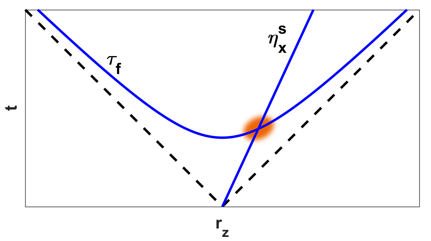
As discussed in [12], for a 1+1 dimensional relativistic source, the longitudinal radius in an arbitrary frame reads as
| (11) |
where is the space-time rapidity, and is the main emission region of the source, which derived by the saddle-point calculation of the rapidity density, and are characteristic sizes around and . This formula simplifies a lot in the LCMS (longitudinally co-moving system) frame of the boson pair, where :
| (12) |
Our new family of solutions are finite, and limited to a narrow rapidity interval around midrapidity [1]. At mid-rapidity, if , the above equation can be simplied even further:
| (13) |
3 Previous results on the longitudinal HBT-radius
For a Hwa-Bjorken type of accelerationless, longitudinal flow [8, 7] Makhlin and Sinyukov determined the longitudinal length of homogeneity in ref. [11] as
| (14) |
In this equation, stands for the freeze-out temperature, is the transverse mass of the particle pair and is the mean freeze-out time of the Hwa-Bjorken solution. This result makes it possible to determine the life-time, i.e. of the reaction from the measurement of the longitudinal HBT radius parameter, provided that MeV can be estimated from the analysis of the single particle spectra.
Evaluating the HBT radii from the same Hwa-Bjorken solution [8, 7], Herrmann and Bertsch obtained a more accurate result in ref. [14], using a Gaussain approximation for the longitudinal HBT radius at midrapidity, in terms of Bessel functions and , as follows:
| (15) |
This formula improves the Sinyukov-Makhlin formula (14) for lower values, and approaches it in the large limit.
If the flow is accelerating, the estimated origin of the trajectiories is shifted back in proper-time, thus is underestimating the life-time of the reaction. The correction was estimated, based on the modification of the flow-profile, from the Csörgő-Nagy-Csanád (CNC) solution [10] as follows
| (16) |
where stands for the freeze-out time. In the boost-invariant limit, this formula also reproduces the Makhlin-Sinyukov formula, but for the realistic parameter values it yields larger life-times as compared to the Makhlin-Sinyukov formula.
4 The longitudinal HBT-radius parameter of the CKCJ solution
Let us evaluate the emission function for the CKCJ solution of refs. [1, 2, 3]. The integration of the Cooper-Frye formula is performed by the saddle-point approximation. Near to mid-rapidity, the fluid rapidity is well approximated by a linear function of the space-time rapidity: . Using a saddle-point integration in , we obtain the rapidity distribution:
| (17) |
Here stands for the saddle-point, which is found to be proportional to the rapidity : . At midrapidity, the saddle-point vanishes and the emission function can be well approximated by a Gaussian centered on zero. The width of this Gaussian is given by as
| (18) |
At mid-rapidity, these considerations lead to the following longitudinal HBT-radius parameter:
| (19) |
Surprisingly, this result is independent of the equation of state, and it is formally different from the CNC estimate.
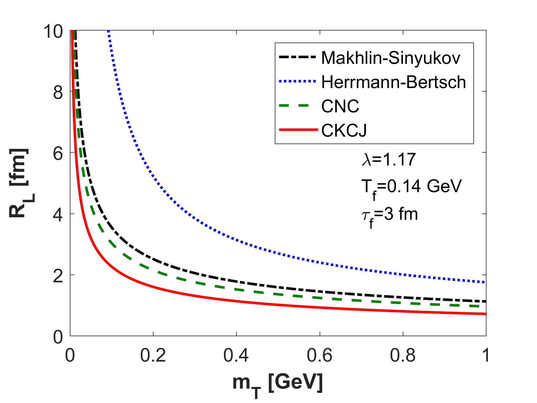
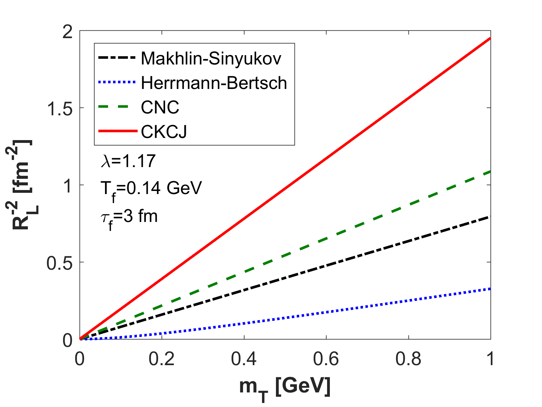
Our result thus presents and important step forward: once the parameter of the acceleration is determined from the fits to the (pseudo)rapidity distributions [2], this parameter combined with the longitudinal HBT radius measurement can be used to provide an advanced estimate of the life-time of the reaction, solving eq. (19) for the life-time . The significance of our advanced formula is illustrated on Figure 2.
Acknowledgments
We greatfully acknowledge partial support form the Hungarian NKIFH grants No. FK-123842 and FK-123959, the Hungarian EFOP 3.6.1-16-2016-00001 project and the exchange programme of the Hungarian and the Ukrainian Academies of Sciences, grants NKM-82/2016 and NKM-92/2017.
References
- [1] T. Csörgő, G. Kasza, M. Csanád and Z. Jiang, Universe 4, 69 (2018)
- [2] T. Csörgő, G. Kasza, M. Csanád and Z. F. Jiang, arXiv:1806.06794 [nucl-th].
- [3] G. Kasza and T. Csörgő, arXiv:1806.11309 [nucl-th].
- [4] T. Csörgő, B. Lörstad and J. Zimányi, Z. Phys. C 71, 491 (1996)
- [5] G. F. Bertsch, Nucl. Phys. A 498, 173C (1989).
- [6] S. Pratt, Phys. Rev. Lett. 53, 1219 (1984).
- [7] J. D. Bjorken, Phys. Rev. D 27 (1983) 140.
- [8] R. C. Hwa, Phys. Rev. D 10, 2260 (1974). doi:10.1103/PhysRevD.10.2260
- [9] T. Csörgő, M. I. Nagy and M. Csanád, Phys. Lett. B 663, 306 (2008)
- [10] M. I. Nagy, T. Csörgő and M. Csanád, Phys. Rev. C 77, 024908 (2008)
- [11] A. N. Makhlin and Y. M. Sinyukov, Z. Phys. C 39, 69 (1988).
- [12] T. Csörgő and B. Lörstad, Phys. Rev. C 54, 1390 (1996)
- [13] T. Csörgő, Acta Phys. Hung. A 15, 1 (2002)
- [14] M. Herrmann and G. F. Bertsch, Phys. Rev. C 51, 328 (1995)