Brown measure support and the free multiplicative Brownian motion

Abstract.

The free multiplicative Brownian motion $b_{t}$ is the large-$N$ limit of Brownian motion $B_{t}^{N}$ on the general linear group $\mathrm{GL}(N;\mathbb{C})$. We prove that the Brown measure for $b_{t}$—which is an analog of the empirical eigenvalue distribution for matrices—is supported on the closure of a certain domain $\Sigma_{t}$ in the plane. The domain $\Sigma_{t}$ was introduced by Biane in the context of the large-$N$ limit of the Segal–Bargmann transform associated to $\mathrm{GL}(N;\mathbb{C})$.

We also consider a two-parameter version, $b_{s,t}$: the large-$N$ limit of a related family of diffusion processes on $\mathrm{GL}(N;\mathbb{C})$ introduced by the second author. We show that the Brown measure of $b_{s,t}$ is supported on the closure of a certain planar domain $\Sigma_{s,t}$, generalizing $\Sigma_{t}$, introduced by Ho.

In the process, we introduce a new family of spectral domains related to any operator in a tracial von Neumann algebra: the $L^{p}_{n}$-spectrum for $n\in\mathbb{N}$ and $p\geq 1$, a subset of the ordinary spectrum defined relative to potentially-unbounded inverses. We show that, in general, the support of the Brown measure of an operator is contained in its $L_{2}^{2}$-spectrum.

1. Introduction

One of the core theorems in random matrix theory is the circular law. Suppose $C^{N}$ is an $N\times N$ complex matrix whose entries are independent centered normal random variables of variance $\frac{1}{N}$. Then the empirical eigenvalue distribution of $C^{N}$ (the random probability measure placing points of equal mass at the eigenvalues) converges almost surely to the uniform probability measure on the unit disk as $N\to\infty$. This theorem is due to Ginibre [18] and $C^{N}$ is often called a Ginibre ensemble. The circular law has been incrementally generalized to its strongest form where the entries are independent but can have any distribution with two finite moments [1, 19, 20, 39].

We can recast this as a theorem about matrix-valued Brownian motion. In a finite-dimensional real Hilbert space, there is a canonical Brownian motion, constructed by adding independent standard real Brownian motions in all the directions of any orthonormal basis. (See Section 2.1.1 below.) Let us regard the space $M_{N}(\mathbb{C})$ of complex $N\times N$ matrices as a real vector space of dimension $2N^{2}$, and equip it with the inner product

$$\left\langle X,Y\right\rangle_{N}=N\operatorname{Re}\mathrm{Trace}(X^{\ast}Y).$$ (1.1)

Then the associated Brownian motion $C^{N}_{t}$ has the same law as the Ginibre ensemble, scaled by a factor of $\sqrt{t}$. (The factor $N$ in front of the Hilbert–Schmidt inner product is the correct choice to give the entries variance of order $1/N$.) Hence, the matrix-valued Brownian motion $C^{N}_{t}$ has eigenvalues that concentrate uniformly in the disk of radius $\sqrt{t}$ as $N\to\infty$.

In this paper, we are interested in the Brownian motion $B^{N}_{t}$ on the general linear group $\mathrm{GL}(N;\mathbb{C})$. One nice geometric way to define this object is by the rolling map. The tangent space to the identity in $\mathrm{GL}(N;\mathbb{C})$ (i.e., the Lie algebra of this Lie group) is all of $M_{N}(\mathbb{C})$. Take the Brownian paths in the tangent space, and roll them onto the group; this yields the paths of $B^{N}_{t}$. Since the paths are not smooth this rolling is accomplished by a stochastic differential equation for $B^{N}_{t}$ in terms of $C^{N}_{t}$ (cf. (2.2)). In particular, for small time, $B^{N}_{t}$ and $C^{N}_{t}$ are ”close”, and so it is natural to expect that the eigenvalues of $B^{N}_{t}$ should follow a deformation of the circular law of radius $\sqrt{t}$.

For a normal matrix $A$, the eigenvalues are encoded in the matrix moments $\{\mathrm{Trace}[A^{k}(A^{\ast})^{\ell}]\}_{k,\ell\in\mathbb{N}}$. However, the ensemble $C^{N}_{t}$ is almost surely non-normal for any $t>0$; in fact, a stronger statement is true: with probability $1$, $C^{N}_{t}$ is non-normal for all $t>0$ [30, Proposition 4.15]. The lack of normality presents significant hurdles to understanding the limit behavior of its eigenvalues, whose connection to matrix moments is quite a bit more subtle. Nevertheless, the $\ast$-moments of $C_{t}^{N}$ and $(C_{t}^{N})^{\ast}$ (i.e., traces of all words in these non-commuting matrices) do have a meaningful large-$N$ limit: in the language of free probability, the ensemble $C^{N}_{t}$ converges in $\ast$-distribution to an operator $c_{t}$, cf. [40] (see Section 2.1.2).

This circular Brownian motion $c_{t}$, living in noncommutative probability space, does not have eigenvalues, and is not normal, so it does not have a spectral resolution. Nevertheless, there is a construction, known as the Brown measure that reproduces the spectral distribution in the normal case but is also valid for non-normal operators. Each operator $a$ in a tracial von Neumann algebra has an associated Brown measure $\mu_{a}$, which is a probability measure supported in the spectrum of $a$ in $\mathbb{C}$. If $a$ is normal, $\mu_{a}$ is the usual spectral measure inherited from the spectral theorem; if $A$ is an $N\times N$ matrix, its Brown measure is simply its empirical eigenvalue distribution. We discuss the Brown measure in general in Section 2.3 below. Girko’s proof [19] of the general circular law begins by proving that the Brown measure of $c_{1}$ is uniform on the unit disk, and then shows that the empirical eigenvalue distribution of $C^{N}$ actually converges to the Brown measure of the large-$N$ limit.

Meanwhile, the Brownian motion $B_{t}^{N}$ on the group $\mathrm{GL}(N;\mathbb{C})$ also has a large-$N$ limit in terms of $\ast$-distribution: an operator $b_{t}$ known as the free multiplicative Brownian motion. It was introduced by Biane [4, 5] and conjectured by him to be the large-$N$ limit of $B_{t}^{N}$; this conjecture was proven by the second author in [30]. The first step in understanding the large-$N$ behavior of the eigenvalues of $B_{t}^{N}$ is to determine the Brown measure $\mu_{b_{t}}$ of $b_{t}$. It is a probability measure supported in the spectrum of $b_{t}$; but $b_{t}$ is a complicated object, and in particular its spectrum is completely unknown.

In this paper, we identify a closed set $\overline{\Sigma}_{t}$ (see Section 2.2) which contains the support of the Brown measure $\mu_{b_{t}}$. The region $\Sigma_{t}$ was introduced by Biane in [5] in the context of the Segal–Bargmann transform (or “Hall transform”) associated to the unitary group $\mathrm{U}(N)$ and its complexification $\mathrm{GL}(N;\mathbb{C})$ (cf. [23]). Biane introduced a free Hall transform $\mathscr{G}_{t}$, which he understood as a sort of large-$N$ limit of the Hall transform for $\mathrm{U}(N)$. The transform $\mathscr{G}_{t}$ is an integral operator which maps functions on the unit circle to a space $\mathscr{A}_{t}$ of holomorphic functions on the region $\Sigma_{t}\subset\mathbb{C}$, whose definition falls out of the complex analysis used in Biane’s proofs.

The meaning of the region $\Sigma_{t}$ and its relation to the free multiplicative Brownian motion $b_{t}$ have remained mysterious. One clue to its origin comes from the holomorphic functional calculus. Using the metric properties of $\mathscr{G}_{t}$, Biane showed that one can make sense of $F(b_{t})$, as a possibly unbounded operator, for any $F\in\mathscr{A}_{t}$. Now, if the spectrum of $b_{t}$ were contained in $\Sigma_{t}$, properties of the holomorphic functional calculus would show that $F(b_{t})$ is a bounded operator for all $F$ in $\mathcal{H}(\Sigma_{t})$ and thus for all $F$ in $\mathscr{A}_{t}$, which is (presumably) not the case. On the other hand, the fact that $F(b_{t})$ can be defined at all — even as an unbounded operator — suggests that the spectrum of $b_{t}$ is at least contained in the closure of $\Sigma_{t}$. Such a results would then imply that the support of the Brown measure of $b_{t}$ is contained in $\overline{\Sigma}_{t}$. The latter statement is the main theorem of this paper.

Theorem 1.1.

For all $t>0$, the support of the Brown measure $\mu_{b_{t}}$ of the free multiplicative Brownian motion $b_{t}$ is contained in $\overline{\Sigma}_{t}$.

We expect that the large-$N$ limit of the empirical eigenvalue distribution of the Brownian motion $B_{t}^{N}$ on $\mathrm{GL}(N;\mathbb{C})$ coincides with the Brown measure $\mu_{b_{t}}$ of the free multiplicative Brownian motion. If that is the case, the eigenvalues of $B_{t}^{N}$ should concentrate in $\overline{\Sigma}_{t}$ for large $N$; this claim is supported by numerical evidence. Figure 1 shows simulations of $B_{t}^{N}$ with $N=2000$ and four different values of $t$, plotted along with the domains $\Sigma_{t}$. (The domain for $t\geq 4$ has a small hole around the origin, which can be seen in the bottom two images in the figure.)

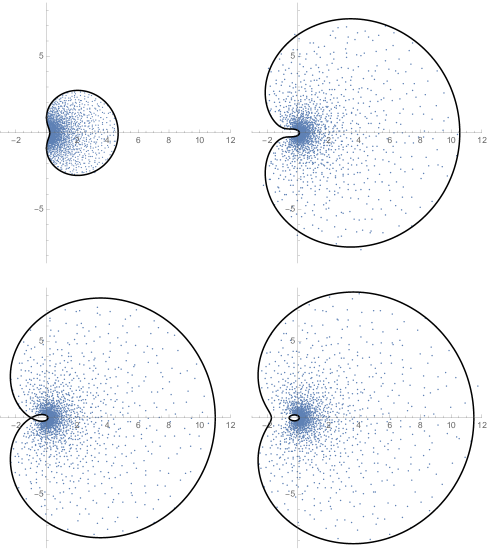
Figure 1. Simulations of the eigenvalues of $B_{t}^{N}$ shown with the domain $\Sigma_{t}$, for $N=2000$ and $t=2$, $t=3.9$, $t=4$, and $t=4.1$

We also consider a two-parameter version $b_{s,t}$ of the free multiplicative Brownian motion and show that its Brown measure is supported on the closure of a certain domain $\Sigma_{s,t}$, introduced by Ho [29]. These domains similarly arise in the large-$N$ limit of the two-parameter Segal–Bargmann transform in the Lie group setting. The precise statement and proof can be found in Section 5.

After this paper was submitted for publication, we became aware of two papers in the physics literature that address the large-$N$ limit of Brownian motion in $GL(N;\mathbb{C}).$ The first, by Gudowska-Nowak, Janik, Jurkiewicz, Nowak [36] addresses only the one-parameter case (what we call $B_{t}^{N}$). The second, by Lohmayer, Neuberger, and Wettig [32] addresses the full two-parameter case (what we call $B_{s,t}^{N}$ in Section 5). Using nonrigorous methods, both papers identify the region in which the eigenvalues should live in the large-$N$ limit. The domains they identify are precisely what we call $\Sigma_{t}$ (in the one-parameter case in [36]) and what we call $\Sigma_{s,t}$ (in the two-parameter case in [32]).

Our results are rigorous and use completely different methods from those in [36, 32]. Our approach also has the conceptual advantage of connecting the Brown measure of the free multiplicative Brownian motion to the previously known results on the distribution of the free unitary Brownian motion. Finally, we develop a general result about Brown measures and the notion of $L_{2}^{2}$ spectrum. (For more details on the relationship between [36, 32] and our results, see Remark 5.5 below.)

The strategy we employ to prove Theorem 1.1 is of independent interest, as it provides a new restriction on the support of the Brown measure of an operator, in terms of a family of spectral domains associated to the operator. Let $(\mathcal{A},\tau)$ be a tracial von Neumann algebra and let $a\in\mathcal{A}$. As noted, the Brown measure $\mu_{a}$ is supported in the spectrum of $a$; in fact, its support set may be a strict subset of the spectrum. Recall that the spectrum of $a$ is the complement of the resolvent set of of $a$, which is the set of $\lambda\in\mathbb{C}$ for which $a-\lambda$ is invertible (meaning that $(a-\lambda)^{-1}$ is a bounded operator). The rich structure of $\mathcal{A}$ and the trace $\tau$ give a natural generalization of these spaces: we may ask that the inverse $(a-\lambda)^{-1}$ exist but not necessarily be bounded, instead insisting that it is in $L^{p}(\mathcal{A},\tau)$ for some $p\geq 1$. (The $p=\infty$ case coincides with the usual resolvent set.) What is more, given the often bizarre algebraic properties of non-normal operators (which can, for example, be nilpotent), we may ask that some power $(a-\lambda)^{n}$ have an inverse in $L^{p}(\mathcal{A},\tau)$. (Unless $a$ is normal, this is not equivalent to $a-\lambda$ having an inverse in $L^{np}(\mathcal{A},\tau)$.) The set of $\lambda\in\mathbb{C}$ for which $(a-\lambda)^{n}$ has an inverse in $L^{p}$ (and for which certain uniform local bounds hold) is called the $L^{p}_{n}$-resolvent set of $a$, and its complement is $\mathrm{spec}^{p}_{n}(a)$, the $L^{p}_{n}$-spectrum of $a$.

Our key observation leading to the proof of Theorem 1.1 is the following new description of (a closed set containing) the support of the Brown measure.

Theorem 1.2.

For any operator $a$ in a tracial von Neumann algebra, the support of the Brown measure $\mu_{a}$ is contained in $\mathrm{spec}^{2}_{2}(a)$, which is a subset of the spectrum of $a$.

A detailed discussion of these generalized spectral domains, and the proof of Theorem 1.2, can be found in Section 6.1. Once this result is established, we use Biane’s free Hall transform $\mathscr{G}_{t}$ to show that $\mathrm{spec}_{2}^{2}(b_{t})=\overline{\Sigma}_{t}$, which proves that the support of $\mu_{b_{t}}$ is contained in $\overline{\Sigma}_{t}$, establishing Theorem 1.1.

A more detailed version of this outline of the proof is contained in Section 4, (cf. Theorems 4.1 and 4.2); the complete proofs can then be found in Section 6.

2. Preliminaries

In this section, we provide background on the objects in the statement of our main theorem—the free multiplicative Brownian motion, the Brown measure, and the domains $\Sigma_{t}$.

2.1. Lie group Brownian motions and their large-$N$ limits

2.1.1. Lie group Brownian motions

Let $H$ be a finite-dimensional real Hilbert space. The Brownian motion on $H$, $W^{H}_{t}$, is the diffusion process defined by

$$W^{H}_{t}=\sum_{j=1}^{d}B^{j}_{t}e_{j}$$ (2.1)

where $\{e_{1},\ldots,e_{d}\}$ is an orthonormal basis for $H$, and $\{B^{j}_{t}\}_{j=1}^{d}$ are i.i.d. standard (real) Brownian motions. The law of this process is invariant under rotations, and hence does not depend on which orthonormal basis is chosen.

Let $G\subset\mathrm{GL}(N;\mathbb{C})$ be a matrix Lie group (in $M_{N}(\mathbb{C})$), and let $\mathfrak{g}\subset M_{N}(\mathbb{C})$ be its Lie algebra. A choice of inner product on $\mathfrak{g}$ induces a left-invariant Riemannian metric on $G$. As a Riemannian manifold, then, $G$ has a well-defined Brownian motion: the diffusion with infinitesimal generator given by half the Laplacian. In the Lie group setting there is a simple description of the Brownian motion $B^{G}_{t}$ in terms of the Brownian motion $W^{\mathfrak{g}}_{t}$ on the Lie algebra (as in (2.1)):

$$dB^{G}_{t}=B^{G}_{t}\circ dW^{\mathfrak{g}}_{t},\qquad B^{G}_{0}=I.$$ (2.2)

The $\circ$ denotes the Stratonovich stochastic integral. This Stratonovich SDE can be converted to an Itô SDE; the form of the resulting equation depends on the structure of the group (cf. [33, p. 116]).

For our purposes, the two relevant Lie groups are the unitary group $\mathrm{U}(N)$ whose Lie algebra is $\mathfrak{u}(N)=M_{N}^{\mathrm{s.a.}}(\mathbb{C})$ (self-adjoint matrices), and the general linear group $\mathrm{GL}(N;\mathbb{C})$ whose Lie algebra consists of all complex matrices $\mathfrak{gl}(N;\mathbb{C})=M_{N}(\mathbb{C})$. (In the unitary case, we follow the physicists’ convention; mathematicians typically use skew-self-adjoint matrices.) Using the inner product (1.1) on both these Lie algebras, we obtain Brownian motions which we will denote thus:

$$W^{\mathfrak{u}(N)}_{t}=X^{N}_{t}\qquad\text{and}\qquad W^{\mathfrak{gl}(N;\mathbb{C})}_{t}=C^{N}_{t}.$$

To be more explicit, $C^{N}_{t}$ is the Ginibre Brownian motion, which has i.i.d. entries that are all complex Brownian motions of variance $t/N$, and $X^{N}_{t}$ is the Wigner Brownian motion, which is Hermitian with i.i.d. upper triangular entries, with complex Brownian motions above the diagonal and real Brownian motions on the diagonal, each of variance $t/N$.

The Brownian motions on the groups, which we denote $B^{\mathrm{U}(N)}_{t}=U^{N}_{t}$ and $B^{\mathrm{GL}(N;\mathbb{C})}_{t}=B^{N}_{t}$, then satisfy Stratonovich SDEs given by (2.2). These equations can be written in Itô form as follows:

$$dU^{N}_{t}=iU^{N}_{t}\,dX^{N}_{t}-\textstyle{\frac{1}{2}}U^{N}_{t}\,dt\qquad\text{and}\qquad dB^{N}_{t}=B^{N}_{t}\,dC^{N}_{t}$$ (2.3)

(both started at the identity matrix). These defining SDEs play the role of the rolling map described in the introduction.

2.1.2. The large-$N$ limits

The four processes $X^{N}_{t}$, $C^{N}_{t}$, $U^{N}_{t}$, and $B^{N}_{t}$ all have large-$N$ limits in the sense of free probability theory. (For a thorough introduction to free probability theory and its connection to random matrix theory, the reader is directed to [34] and [35].) The limits are one-parameter families of operators $x_{t}$, $c_{t}$, $u_{t}$, and $b_{t}$ all living in a noncommutative probability space $(\mathcal{B},\tau)$. (More precisely, $\mathcal{B}$ is a finite von Neumann algebra and $\tau$ is a faithful, normal, tracial state.) The sense of convergence is almost sure convergence of the finite-dimensional noncommutative distributions, defined as follows.

Definition 2.1.

Let $A^{N}_{t}$ be a sequence of $M_{N}(\mathbb{C})$-valued stochastic processes (all defined on the same sample space). Let $(\mathcal{A},\tau)$ be a noncommutative probability space, and let $a_{t}\in\mathcal{A}$ for each $t>0$. We say $A^{N}_{t}$ converges to $a_{t}$ in finite-dimensional noncommutative distributions if, for each $n\in\mathbb{N}$ and times $t_{1},\ldots,t_{n}\geq 0$, and each noncommutative polynomial $P$ in $2n$ indeterminates, then almost surely

$$\lim_{N\to\infty}\textstyle{\frac{1}{N}}\mathrm{Trace}\!\left[P(A^{N}_{t_{1}},\ldots,A^{N}_{t_{n}},(A^{N}_{t_{1}})^{\ast},\ldots,(A^{N}_{t_{n}})^{\ast})\right]=\tau\!\left[P(a_{t_{1}},\ldots,a_{t_{n}},a_{t_{1}}^{\ast},\ldots,a_{t_{n}}^{\ast})\right].$$

The limit of $X^{N}_{t}$ was identified by Voiculescu [40]; it is known as free additive Brownian motion $x_{t}$, and can be constructed on a Fock space. From here, one can derive the $C^{N}_{t}$ case by noting that $C^{N}_{t}=\frac{1}{\sqrt{2}}(X^{N}_{t}+iY^{N}_{t})$ where $Y^{N}_{t}$ is an independent copy of $X^{N}_{t}$. Given the independence and rotational invariance, it follows by standard results on asymptotic freeness that the large-$N$ limit of $C^{N}_{t}$ can be represented as $c_{t}=\frac{1}{\sqrt{2}}(x_{t}+iy_{t})$ where $\{x_{t},y_{t}\}$ are freely independent free additive Brownian motions; we call $c_{t}$ a free circular Brownian motion.

Since the unitary and general linear Brownian motions $U^{N}_{t}$ and $B^{N}_{t}$ are defined as solutions of SDEs involving $X^{N}_{t}$ and $C^{N}_{t}$, good candidates for their large-$N$ limits are given by free SDEs involving $x_{t}$ and $c_{t}$. (Free stochastic analysis was introduced in [7] and further developed in [8, 31]; the reader may also consult the background sections of [12, 30] for succinct summaries of the relevant concepts.) The free unitary Brownian motion $u_{t}$ and free multiplicative Brownian motion $b_{t}$ are defined as solutions to the free SDEs

$$du_{t}=iu_{t}\,dx_{t}-\textstyle{\frac{1}{2}}u_{t}\,dt\qquad\text{and}\qquad db_{t}=b_{t}\,dc_{t}$$ (2.4)

(both started at $1$), mirroring the matrix SDEs of (2.3).

The free unitary Brownian motion $u_{t}$ was introduced by Biane in [4], wherein he also showed that it is the large-$N$ limit of the unitary Brownian motion $U^{N}_{t}$ as a process (as in Definition 2.1). In particular, in the case of a single time $t$ ($n=1$ in the definition, $t_{1}=t$), since $u_{t}^{\ast}=u_{t}^{-1}$, the statement is simply that the trace moments $\frac{1}{N}\mathrm{Trace}[(U_{t}^{N})^{k}]$, $k\in\mathbb{Z}$, converge almost surely as $N\to\infty$ to $\tau[u_{t}^{k}]$. The numbers $\nu_{k}(t):=\tau[u_{t}^{k}]$, meanwhile, are the moments of a probability measure $\nu_{t}$ on the unit circle. Biane computed these limit moments, which had already appeared in work of Singer [38] in Yang–Mills theory on the plane in an asymptotic regime. They are given by

$$\nu_{k}(t):=\int_{\partial\mathbb{D}}\omega^{k}~{}\nu_{t}(d\omega)=e^{-\frac{\left|k\right|}{2}t}\sum_{j=0}^{\left|k\right|-1}\frac{(-t)^{j}}{j!}\left|k\right|^{j-1}\binom{\left|k\right|}{j}$$ (2.5)

for $n\in\mathbb{Z}\setminus\{0\}$, with $\nu_{0}(t)=1$.

From here, using complex analytic techniques, Biane completely determined the measure $\nu_{t}$. For $t>4$, the support of $\nu_{t}$ is the whole unit circle while for $t<4$ its support is the following arc:

$$\mathrm{supp}\,\nu_{t}=\left\{e^{i\theta}\colon|\theta|\leq\frac{1}{2}\sqrt{t(4-t)}+\arccos\left(1-\frac{t}{2}\right)\right\},\quad t<4.$$ (2.6)

Biane also gave an implicit description of the measure $\nu_{t}$, which has a real analytic density on the interior of its support, but we do not need this description presently.

The key to analyzing $\nu_{t}$ was determining a certain analytic transform of $\nu_{t}$ in the unit disk $\mathbb{D}$. Let

$$\psi_{t}(z):=\int_{\partial\mathbb{D}}\frac{\omega z}{1-\omega z}\,\nu_{t}(d\omega),\qquad z\in\mathbb{D}$$

denote the moment generating function (with no constant term). The function $\psi_{t}$ has a continuous extension to the closed disk $\overline{\mathbb{D}}$; this is tantamount to the fact, as Biane proved, that $\nu_{t}$ possesses a continuous density on $\partial\mathbb{D}$. Of greater computational use is the following function:

$$\chi_{t}(z):=\frac{\psi_{t}(z)}{1+\psi_{t}(z)}$$ (2.7)

which also has a continuous extension to $\overline{\mathbb{D}}$. In fact, $\chi_{t}$ is one-to-one on the open disk, and its inverse is analytic, with the following simple explicit formula:

$$f_{t}(z):=\chi_{t}^{\langle-1\rangle}(z)=ze^{\frac{t}{2}\frac{1+z}{1-z}}.$$ (2.8)

It is from this identity that the explicit formulas (2.5) and (2.6) are derived.

Biane also introduced the free multiplicative Brownian motion process $b_{t}$ in [5], where he conjectured that it is the large-$N$ limit of the $\mathrm{GL}(N;\mathbb{C})$ Brownian motion $B^{N}_{t}$. Given the non-normality of the matrices and operators involved, this turned out to be a difficult problem that took nearly two decades to solve; the second author proved this in [30]. Now, the “holomorphic” moments $\tau[b_{t}^{k}]$ are easily shown to have the value $1$ for all $k$ (see also (5.6)). But since the process $b_{t}$ is not normal, these moments do not determine much of the noncommutative distribution. The free SDE (2.4) that defines $b_{t}$ allows for any mixed moment in $b_{t}$ and $b_{t}^{\ast}$ to be computed (iteratively) given enough patience; see [30, Proposition 1.8] for some notable examples. There is, at present, no known simple description of the full noncommutative distribution of this complicated object. Its spectrum is also unknown.

2.2. The domains $\Sigma_{t}$

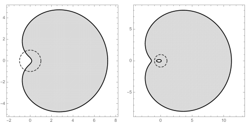
Figure 2. The domains $\Sigma_{t}$ with $t=3$ and $t=4.05$, with the unit circle (dashed) shown for comparison

In this section, we describe the family of domains $\Sigma_{t}\subset\mathbb{C}$, introduced by Biane in [5], which enter into the statement of our main result. They arose in the context of the free Segal–Bargmann transform (see Section 3), which connects $u_{t}$ and $b_{t}$. For this reason, they are related to the function $f_{t}$ in (2.8), which is the inverse of the shifted moment generating function of the spectral measure $\nu_{t}$ of the free unitary Brownian motion.

It is easily verified that if $\left|z\right|=1$, then $\left|f_{t}(z)\right|=1$. There are, however, points $z$ with $\left|z\right|\neq 1$ for which $\left|f_{t}(z)\right|$ is nevertheless equal to 1.

Proposition 2.2.

For all $t>0$, consider the set

$$E_{t}=\overline{\left\{z\in\mathbb{C}\left|\left|z\right|\neq 1,~{}\left|f_{t}(z)\right|=1\right.\right\}}$$

and define $\Sigma_{t}$ to be the connected component of the complement of $E_{t}$ containing 1. Then $\Sigma_{t}$ is bounded for all $t>0$, $\Sigma_{t}$ is simply connected for $t\leq 4$, and $\Sigma_{t}$ is doubly connected for $t>4$. In all cases, we have

$$\partial\Sigma_{t}=E_{t}.$$

These properties of the region $\Sigma_{t}$ were proved by Biane in [5]; see especially pp. 273–274. See also [29, Section 4.2]. The closure in the definition of the set $E_{t}$ is needed to fill in the points (at most two of them) where $\partial\Sigma_{t}$ intersects the unit circle. In recent joint work between the present authors and Driver [15, Theorem 4.1], we found a simpler description of the regions $\Sigma_{t}$. They are the level sets of a certain explicit function: $\Sigma_{t}=\{\lambda\in\mathbb{C}\colon T(\lambda)<t\}$ and $\partial\Sigma_{t}=\{\lambda\in\mathbb{C}\colon T(\lambda)=t\}$, where

$$T(\lambda)=|\lambda-1|^{2}\frac{\log(|\lambda|^{2})}{|\lambda|^{2}-1}.$$

(It is easy to compute that this expression has a limit as $|\lambda|\to 1$. Indeed, $T$ extends to a real analytic function on $\mathbb{C}\setminus\{0\}$, and for $|\lambda|=1$, we have $T(\lambda)=|\lambda-1|^{2}$.) Figure 2 shows the domain $\Sigma_{t}$ with $t=3$ and $t=4.05$, with the unit circle shown for comparison. Figure 3 then shows the transitional case $t=4$ in more detail. In all cases, 1 is in $\Sigma_{t}$ and 0 is not in $\overline{\Sigma}_{t}$.

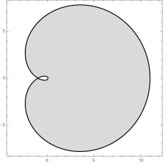
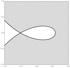
Figure 3. The region $\Sigma_{t}$ with $t=4$ (left) and a detail thereof (right)

An important property of the region $\Sigma_{t}$, which follows from the just-cited results of Biane [5], involves the support arc of the spectral measure $\nu_{t}$ of free unitary Brownian motion. This result is crucial to the proof of our main theorem.

Proposition 2.3.

For all $t>0$, the function $f_{t}$ maps $\mathbb{C}\setminus\overline{\Sigma}_{t}$ injectively onto $\mathbb{C}\setminus\mathrm{supp}\,\nu_{t}$.

This is a typical “slit plane” conformal map; see Figure 4.

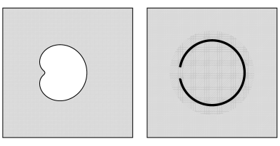
Figure 4. The map $f_{t}$ takes $\mathbb{C}\setminus\overline{\Sigma}_{t}$ (left) injectively onto $\mathbb{C}\setminus\mathrm{supp}\,\nu_{t}$ (right). Shown for $t=3$

2.3. Brown measure

We work in the context of a sufficiently rich noncommutative probability space: a tracial von Neumann algebra.

Definition 2.4.

A tracial von Neumann algebra is a finite von Neumann algebra $\mathcal{A}$ together with a faithful, normal, tracial state $\tau:\mathcal{A}\rightarrow\mathbb{C}$.

Recall that a state $\tau$ is norm-$1$ linear functional taking non-negative elements to non-negative real numbers. (Such a functional necessarily satisfies $\tau(1)=\|\tau\|=1$.) A state $\tau$ is called faithful if $\tau(a^{*}a)>0$ for all $a\neq 0$, it is called normal if it is continuous with respect to the weak^∗ topology on $\mathcal{A}$ (cf. [9, Theorem III. 2.1.4, p. 262]), and it is called tracial if $\tau(ab)=\tau(ba)$ for all $a,b\in\mathcal{A}$.

Let $(\mathcal{A},\tau)$ be a tracial von Neumann algebra. For each element $a$ of $\mathcal{A}$, it is possible to define a probability measure $\mu_{a}$ on $\mathbb{C}$ called the Brown measure of $a$, which should be interpreted as something like an empirical eigenvalue distribution for the operator $a$. The definitions and properties stated in this section may be found in Brown’s original paper [10] and in [34, Chapter 11].

We first recall the notion of the Fuglede–Kadison determinant of $a$ [16, 17], denoted $\Delta(a)$, which is most easily defined by a limiting process:

$$\log\Delta(a)=\lim_{\varepsilon\rightarrow 0}\frac{1}{2}\tau[\log(a^{\ast}a+\varepsilon)].$$ (2.9)

In general, $\log\Delta(a)$ may have the value $-\infty$, in which case, $\Delta(a)=0$. If, for example, $\mathcal{A}=M_{N}(\mathbb{C})$ and $\tau$ is the normalized trace, then $\Delta(a)=\left|\det a\right|^{1/N}$, where $\det a$ is the ordinary determinant of $a$.

For a tracial von Neumann algebra $(\mathcal{A},\tau)$, the Brown measure of an element $a\in\mathcal{A}$ is then defined as

$$\mu_{a}=\frac{1}{2\pi}\nabla_{\lambda}^{2}\log(\Delta(a-\lambda)),$$

where $\nabla_{\lambda}^{2}$ is the Laplacian with respect to $\lambda$, computed in the distributional sense. It can be shown that this distributional Laplacian is a represented by a probability measure on the plane.

Proposition 2.5.

Let $a$ be an element of $\mathcal{A}$ and let $\mu_{a}$ be its Brown measure. Then the following results hold.

1. The measure $\mu_{a}$ is a probability measure on the plane.

2. The support of $\mu_{a}$ is contained in the spectrum of $a$, but the two sets do not coincide in general.

3. For all non-negative integers $n$,

   $$\int z^{n}~{}d\mu_{a}(z)=\tau[a^{n}],$$

   and if $a$ is invertible, the same result holds for all integers $n$.

Although the support of the Brown measure can be a proper subset of the spectrum, there are many interesting examples in which the two sets coincide.

Using the limiting formula (2.9) for the Flugede–Kadison determinant, we may give a limiting formula for the Brown measure. With the notation

$$a_{\lambda}:=a-\lambda,$$

we have

$$\mu_{a}=\frac{1}{4\pi}\lim_{\varepsilon\rightarrow 0}\left\{\nabla_{\lambda}^{2}\tau[\log(a_{\lambda}^{\ast}a_{\lambda}+\varepsilon)]~{}d^{2}\lambda\right\},$$ (2.10)

where $d^{2}\lambda$ is the two-dimensional Lebesgue measure on $\mathbb{C}$ and the limit is in the weak sense. Furthermore, the Laplacian on the right-hand side of (2.10) can be computed explicitly [34, Section 11.5], giving still another formula for the Brown measure:

$$\mu_{a}=\frac{1}{\pi}\lim_{\varepsilon\rightarrow 0}\left\{\varepsilon~{}\tau[(a_{\lambda}^{\ast}a_{\lambda}+\varepsilon)^{-1}(a_{\lambda}a_{\lambda}^{\ast}+\varepsilon)^{-1}]~{}d^{2}\lambda\right\}.$$ (2.11)

The following result follows easily from (2.11).

Corollary 2.6.

Suppose the quantity

$$\tau[(a_{\lambda}^{\ast}a_{\lambda}+\varepsilon)^{-1}(a_{\lambda}a_{\lambda}^{\ast}+\varepsilon)^{-1}]$$ (2.12)

is bounded uniformly for all $\varepsilon>0$ and all $\lambda$ in a neighborhood of some value $\lambda_{0}$. Then $\lambda_{0}$ does not belong to the support of the Brown measure $\mu_{a}$.

In particular, if $\lambda_{0}$ belongs to the resolvent set of $a$, it is not hard to see that the quantity (2.12) has a finite limit as $\varepsilon\to 0$, for all $\lambda$ in a neighborhood of $\lambda_{0}$, so that the corollary applies. Thus, Corollary 2.6 implies Point 2 of Proposition 2.5. But the corollary is stronger, in the sense that it may apply even if $\lambda_{0}$ is in the spectrum of $a$.

We close this section by noting three important special cases of the Brown measure.

• When $\mathcal{A}=M_{N}(\mathbb{C})$ and $\tau$ is the normalized trace, the Brown measure of a matrix $A$ is its empirical eigenvalue distribution. That is,

  $$\mu_{A}=\frac{1}{N}\sum_{j=1}^{n}\delta_{\lambda_{j}},$$

  where $\lambda_{1},\ldots,\lambda_{N}$ are the eigenvalues of $A$, listed with their algebraic multiplicity.

• For a normal element $a$ of $\mathcal{A}$, Brown measure coincided with the spectral measure: $\mu_{a}$ is just the composition of the projection-valued spectral resolution with $\tau$:

  $$\mu_{a}(V)=\tau(E^{a}(V)),\qquad V\in\mathrm{Borel}(\mathbb{C}),$$

  where $E^{a}$ is the projection-valued measure associated to $a$ by the spectral theorem.

• $\mathscr{R}$-diagonal operators form an important class of (generally) non-normal elements of a tracial von Neumann algebra; these include the circular operators $c_{t}$ and Haar unitaries. An element $a\in\mathcal{A}$ is $\mathscr{R}$-diagonal if it has the same non-commutative distribution as $ua$ for any Haar unitary operator $u$ freely independent from $a$; see [35, Lecture 15] for more details. In [22], Haagerup and Larsen proved that the Brown measure of an $\mathscr{R}$-diagonal operator is rotationally invariant, with a radial real analytic density supported on a certain annulus (or circle) determined by $a$; see the discussion following Theorem 6.2 below for more details.

Since the free multiplicative Brownian motion $b_{t}$ is not finite-dimensional, normal, or $\mathscr{R}$-diagonal, none of the preceding cases applies. We will see, however, that some of the ideas related to the support of the Brown measure of $\mathscr{R}$-diagonal operators are useful in the present context.

3. Free Segal–Bargmann transform

Recall from the Section 2.1 that the law $\nu_{t}$ of free unitary Brownian motion is a probability measure on the unit circle that represents the limiting empirical eigenvalue distribution for Brownian motion in the unitary group. In [5], Biane introduced a “free Hall transform” $\mathscr{G}_{t}$ that maps $L^{2}(\partial\mathbb{D},\nu_{t})$ into $\mathcal{H}(\Sigma_{t})$, the space of holomorphic functions on the domain $\Sigma_{t}$. In this section, we recall both the original construction of $\mathscr{G}_{t}$ given by Biane and a realization given by the authors together with Driver [14] and Cébron [11]. The transform $\mathscr{G}_{t}$ will be a crucial tool in the proof of our main theorem.

3.1. Using free probability

Let $u_{t}$ be a free unitary Brownian motion and $b_{t}$ a free multiplicative Brownian that is freely independent from $u_{t}$, both living in a tracial von Neumann algebra $(\mathcal{B},\tau)$. In the approach pioneered by Biane and further developed by Cébron, the map $\mathscr{G}_{t}$ is characterized by the requirement that for each Laurent polynomial $p$, we have

$$(\mathscr{G}_{t}p)(b_{t})=\tau[p(b_{t}u_{t})|b_{t}],$$ (3.1)

where $\tau[\,\cdot\,|b_{t}]$ is the conditional trace with respect to the algebra generated by $b_{t}$. (Compare [5, Theorem 8] for a strictly unitary analog, and [11, Theorem 3] for the precise statement of (3.1).) If, for example, $p$ is the polynomial $p(u)=u^{2}$, then it is not hard to compute (cf. [34, p. 55]) that

$$\tau[b_{t}u_{t}b_{t}u_{t}|b_{t}]=\tau(u_{t})^{2}b_{t}^{2}+(\tau(u_{t}^{2})-\tau(u_{t})^{2})\tau(b_{t})b_{t}.$$

We may then use the moment formulas $\tau(u_{t})=e^{-t}$, $\tau(u_{t}^{2})=e^{-t}(1-t)$, and $\tau(b_{t})=1$. (The moments of $u_{t}$ are the constants $\nu_{k}(t)$ of (2.5), while the moments of $b_{t}$ are the $s=t$ case of (5.6).) We therefore obtain

$$\tau[b_{t}u_{t}b_{t}u_{t}|b_{t}]=e^{-t}(b^{2}-tb).$$

Thus, in this case, $\mathscr{G}_{t}p$ is also a polynomial, given by

$$(\mathscr{G}_{t}p)(b)=e^{-t}(b^{2}-tb).$$ (3.2)

As explained in Section 3.3, the map $\mathscr{G}_{t}$ can be viewed as the large-$N$ limit of the generalized Segal–Bargmann transform over $\mathrm{U}(N)$ introduced by the first author in [23]. The motivation for Biane’s definition of $\mathscr{G}_{t}$ is the stochastic approach to the generalized Segal–Bargmann transform developed by Gross and Malliavin [21].

3.2. As an integral operator

Using the subordination method developed in [6], Biane realized $\mathscr{G}_{t}$ as an integral operator mapping $L^{2}(\partial\mathbb{D},\nu_{t})$ into $\mathcal{H}(\Sigma_{t})$. Explicitly,

$$(\mathscr{G}_{t}f)(z)=\int_{\partial\mathbb{D}}f(\omega)\frac{\left|1-\chi_{t}(\omega)\right|^{2}}{(z-\chi_{t}(\omega))(z^{-1}-\overline{\chi_{t}(\omega)})}~{}d\nu_{t}(\omega),\quad z\in\Sigma_{t},$$ (3.3)

where $\chi_{t}$ was defined in (2.7). (See [5, Theorem 8] and the computations that follow it, along with Proposition 13.) Here, for $\omega\in\partial\mathbb{D}$, $\chi_{t}(\omega)$ denotes the value of the unique continuous extension of $\chi_{t}$ to $\overline{\mathbb{D}}$; in other words, it is the limiting value of $\chi_{t}(\zeta)$ as $\zeta\in\mathbb{D}$ approaches $\omega$ from inside the unit disk. Note that for $\omega\in\partial\mathbb{D}$ both $\chi_{t}(\omega)$ and $1/\overline{\chi_{t}(\omega)}$ lie on the boundary of $\Sigma_{t}$, so that the integrand in (3.3) is a holomorphic function of $z$ for $z$ in the open set $\Sigma_{t}$. Biane showed that, for $t\neq 4$, the map $\mathscr{G}_{t}$ is injective, so that it is possible to identify $L^{2}(\partial\mathbb{D},\nu_{t})$ with its image:

$$\mathscr{A}_{t}:=\mathrm{Image}(\mathscr{G}_{t})\subset\mathcal{H}(\Sigma_{t}).$$

Now, let us define $L_{\mathrm{hol}}^{2}(b_{t},\tau)$ to be the closure in the noncommutative $L^{2}$ space $L^{2}(\mathcal{B},\tau)$ of the space of elements of the form $p(b_{t})$, where $p$ is a Laurent polynomial in one variable. That is to say, $L_{\mathrm{hol}}^{2}(b_{t},\tau)$ is the closure of the span of the positive and negative integer powers of $b_{t}$, not including any powers of $b_{t}^{\ast}$. (Biane used a slightly different definition that is easily seen to be equivalent to this one.) Biane showed that for $t\neq 4$, there is a bijection between $\mathscr{A}_{t}$ and $L_{\mathrm{hol}}^{2}(b_{t},\tau)$ uniquely determined by the condition that for each Laurent polynomial $p$, we have

$$p\mapsto p(b_{t}).$$

Note that for $t\neq 4$, the space $L_{\mathrm{hol}}^{2}(b_{t},\tau)$ is identified with the space $\mathscr{A}_{t}$ of holomorphic functions. Nevertheless, the noncommutative $L^{2}$ norm on $L_{\mathrm{hol}}^{2}(b_{t},\tau)$ does not correspond to an $L^{2}$ norm on $\mathscr{A}_{t}$ with respect to any measure on $\Sigma_{t}$. (It is, instead, the Hilbert space norm induced by a certain reproducing kernel on $\mathscr{A}_{t}$ which is defined by the integral kernel of $\mathscr{G}^{t}$, cf. (3.3).)

For a general $f\in\mathscr{A}_{t}$, we will write the corresponding element of $L_{\mathrm{hol}}^{2}(b_{t},\tau)$ suggestively as $f(b_{t})$ and think of the map $f\mapsto f(b_{t})$ as a variant of the usual holomorphic functional calculus. That is to say, we think of the map from $\mathscr{A}_{t}$ to $L_{\mathrm{hol}}^{2}(b_{t},\tau)$ as “evaluation on $b_{t}$.” Note, however, that elements of $L_{\mathrm{hol}}^{2}(b_{t},\tau)$ are in general unbounded operators.

Theorem 3.1 (Biane’s Free Hall Transform).

For all $t>0$ with $t\neq 4$, the map $\mathscr{G}_{t}$ is a unitary isomorphism from $L^{2}(\partial\mathbb{D},\nu_{t})$ to $\mathscr{A}_{t}$, where the norm on $\mathscr{A}_{t}$ is defined by identification with $L_{\mathrm{hol}}^{2}(b_{t},\tau)$. In particular, we have

$$\left\|f\right\|_{L^{2}(\partial\mathbb{D},\nu_{t})}=\tau\{[(\mathscr{G}_{t}f)(b_{t})]^{*}(\mathscr{G}_{t}f)(b_{t})\}$$

for all $f\in L^{2}(\partial\mathbb{D},\nu_{t})$.

When $t=4$, the preceding theorem is not known to hold, because it is not known that $\mathscr{G}_{t}$ is injective. But one still has a theorem, as follows. One considers at first the map $p\mapsto\mathscr{G}_{t}p$ on polynomials and then constructs a map from the space of polynomials into $L_{\mathrm{hol}}^{2}(b_{t},\tau)$ by mapping $p$ to $(\mathscr{G}_{t}p)(b_{t})$. This map is isometric for all $t>0$ and it extends to a unitary map of $L^{2}(\partial\mathbb{D},\nu_{t})$ onto $L_{\mathrm{hol}}^{2}(b_{t},\tau)$; see Section 6.2 for details.

In light of the preceding discussion, we expect that, at least for $t\neq 4$, the spectrum of $b_{t}$ will not be contained in $\Sigma_{t}$. After all, if such a containment held, the operator $f(b_{t})$, $f\in\mathscr{A}_{t}\subset\mathcal{H}(\Sigma_{t})$ would presumably be computable by the holomorphic functional calculus, in which case $f(b_{t})$ would be a bounded operator. But actually, every element of $L_{\mathrm{hol}}^{2}(b_{t},\tau)$ arises as $f(b_{t})$ for some $f\in\mathcal{A}_{t}$, and the elements of $L_{\mathrm{hol}}^{2}(b_{t},\tau)$ are in general unbounded operators.

On the other hand, since we are able to define $f(b_{t})$ for any $f\in\mathscr{A}_{t}$, at least as an unbounded operator, it seems reasonable to expect that the spectrum of $\Sigma_{t}$ is contained in the closure of $\Sigma_{t}$. Our main result, that the Brown measure of $b_{t}$ is supported in $\overline{\Sigma}_{t}$, is a step toward establishing this claim; compare Proposition 2.5.

3.3. From the generalized Segal–Bargmann transform

In 1994, the first author introduced a generalized Segal–Bargmann transform for compact Lie groups [23]. In the case of the unitary group $\mathrm{U}(N)$, the transform, which we denote here as $\mathscr{G}_{t}^{N}$, maps $L^{2}(\mathrm{U}(N),\rho_{t})$ to the space of holomorphic functions in $L^{2}(\mathrm{GL}(N;\mathbb{C}),\gamma_{t})$. (Note: in [23] and follow-up work such as [14], the transform was often denoted $B_{t}$; to avoid clashing with our present notation $B^{N}_{t}$ for the Brownian motion on $\mathrm{GL}(N;\mathbb{C})$, we use $\mathscr{G}_{t}^{N}$ instead for the Segal–Bargmann transform here.) Here $\rho_{t}$ and $\gamma_{t}$ are heat kernel measures—that is, the distributions at time $t$ of Brownian motions on the respective groups, starting at the identity. The transform is defined as

$$\mathscr{G}_{t}^{N}f=(e^{t\Delta/2}f)_{\mathbb{C}},$$ (3.4)

where $\Delta$ is the Laplacian on $\mathrm{U}(N)$, $e^{t\Delta/2}$ is the associated (forward) heat operator, and $(\cdot)_{\mathbb{C}}$ denotes the holomorphic extension of a sufficiently nice function from $\mathrm{U}(N)$ to $\mathrm{GL}(N;\mathbb{C})$. See also [25] for more information. The transform can easily be “boosted” to map matrix-valued functions on $\mathrm{U}(N)$ to holomorphic matrix-valued functions on $\mathrm{GL}(N;\mathbb{C})$ (by acting component-wise; i.e., via $\mathscr{G}^{N}_{t}\otimes\mathbf{1}_{M_{N}(\mathbb{C})}$).

A stochastic approach to the transform was developed by Gross and Malliavin in [21]; this approach played an important role in Biane’s paper [5]. See also [26, 27] for further development of the ideas in [21]. Let $U_{t}^{N}$ and $B_{t}^{N}$ be independent Brownian motions in $\mathrm{U}(N)$ and $\mathrm{GL}(N;\mathbb{C})$ (cf. (2.3)), and let $f$ be a function on $\mathrm{U}(N)$ that admits a holomorphic extension (also denoted $f$) to $\mathrm{GL}(N;\mathbb{C})$. Then we have

$$\mathbb{E}[f(B_{t}^{N}U_{t}^{N})|B_{t}^{N}]=(\mathscr{G}_{t}^{N}f)(B_{t}^{N}).$$ (3.5)

This result, by itself, is not deep. After all, in the finite-dimensional case, the conditional expectation can be computed as an expectation with respect to $U^{N}_{t}$, with $B^{N}_{t}$ treated as a constant. Since $U^{N}_{t}$ is distributed as a heat kernel on $\mathrm{U}(N)$, the left-hand side of (3.5) becomes a convolution of $f$ with the heat kernel, giving the heat kernel in the definition (3.4) of the transform $\mathscr{G}_{t}^{N}$.

The crucial next step in [21] is to regard $U^{N}_{t}$ and $B^{N}_{t}$ as functionals of Brownian motions in the Lie algebra, by solving the relevant versions of the stochastic differential equation (2.2). Using this idea, Gross and Malliavin are able to deduce the properties of the generalized Segal–Bargmann from the previously known properties of the classical Segal–Bargmann transform for an infinite-dimensional linear space, namely the path space in the Lie algebra of $\mathrm{U}(N)$. (We are glossing over certain technical distinctions; the preceding description is actually closer to [27, Theorem 18].) The expression (3.5) was the motivation for Biane’s formula (3.1) in the free case, and just as in [21], Biane was able to obtain properties of the transform $\mathscr{G}_{t}$ from the corresponding linear case.

In [5], Biane conjectured, with an outline of a proof, that the free Hall transform $\mathscr{G}_{t}$ can be realized using the large-$N$ limit of $\mathscr{G}_{t}^{N}$. This conjecture was then verified independently by the authors and Driver in [14] and by Cébron in [11]; see also the expository paper [28].

The limiting process is as follows. Consider the transform $\mathscr{G}_{t}^{N}$ on matrix-valued functions of the form $f(U)$, where $f$ is a function on the unit circle and $f(U)$ is computed by the functional calculus. If, for example, $f$ is the function $f(u)=u^{2}$ on the circle, then we can consider the associated matrix-valued function $f(U)=U^{2}$ on the unitary group $\mathrm{U}(N)$. For any fixed $N$, the transformed function $\mathscr{G}_{t}^{N}(f)$ on $\mathrm{GL}(N;\mathbb{C})$ will no longer be of functional-calculus type. Nevertheless, in the large-$N$ limit, $\mathscr{G}_{t}^{N}$ will map $f(U)$ to the functional-calculus function $(\mathscr{G}_{t}f)(Z)$, $Z\in\mathrm{GL}(N;\mathbb{C})$.

Specifically, if $p$ is a Laurent polynomial, then $\mathscr{G}_{t}p$ is also a Laurent polynomial, and (abusing notation slightly)

$$\mathscr{G}_{t}^{N}(p(U))=(\mathscr{G}_{t}p)(Z)+O(1/N^{2}),\quad Z\in\mathrm{GL}(N;\mathbb{C}),$$

where $O(1/N^{2})$ denotes a term whose norm is bounded by a constant times $1/N^{2}$. See [14, Theorem 1.11] and [11, Theorem 4]. In particular, if $f(U)=U^{2}$, then in light of (3.2), we have

$$(\mathscr{G}_{t}^{N}f)(Z)=e^{-t}(Z^{2}-tZ)+O(1/N^{2}),\quad Z\in\mathrm{GL}(N;\mathbb{C}).$$

(See also Example 3.5 and the computations on p. 2592 of [14].)

4. An outline of the proof of Theorem 1.1

As we pointed out in Proposition 2.5, the Brown measure of an operator $a$ is supported on the spectrum of $a$. We strengthen this result, as follows. Given a noncommutative probability space $(\mathcal{A},\tau)$, we can construct the noncommutative $L^{2}$ space $L^{2}(\mathcal{A},\tau)$, which is the completion of $\mathcal{A}$ with respect to the noncommutative $L^{2}$ inner product, $\left\langle a,b\right\rangle=\tau(b^{\ast}a)$. It makes sense to multiply an element of the noncommutative $L^{2}$ space $L^{2}(\mathcal{A},\tau)$ by an element of $\mathcal{A}$ itself, and the result is again in $L^{2}(\mathcal{A},\tau)$. We say that $a\in\mathcal{A}$ has an inverse in $L^{2}$ if there exists some $b\in L^{2}(\mathcal{A},\tau)$ such that $ab=ba=1$.

Theorem 4.1.

Let $(\mathcal{A},\tau)$ be a tracial von Neumann algebra and let $\lambda_{0}$ be in $\mathbb{C}$. Suppose that $(a-\lambda)^{2}$ has an inverse—denoted $(a-\lambda)^{-2}$—in $L^{2}(\mathcal{A},\tau)$ for all $\lambda$ in a neighborhood of $\lambda_{0}$ and that $\left\|(a-\lambda)^{-2}\right\|_{L^{2}(\mathcal{A},\tau)}$ is bounded near $\lambda_{0}$. Then $\lambda_{0}$ does not belong to the support of the Brown measure $\mu_{a}$.

Note that if $a-\lambda_{0}$ has a bounded inverse—that is, an inverse in $\mathcal{A}$—then $a-\lambda$ also has an inverse for all $\lambda$ in a neighborhood of $\lambda_{0}$, and $\left\|(a-\lambda)^{-1}\right\|_{\mathcal{A}}$ is bounded near $\lambda_{0}$. In that case, we have

$$\left\|(a-\lambda)^{-2}\right\|_{L^{2}(\mathcal{A},\tau)}\leq\left\|(a-\lambda)^{-2}\right\|_{\mathcal{A}}\leq\left\|(a-\lambda)^{-1}\right\|_{\mathcal{A}}^{2},$$

which shows that $\left\|(a-\lambda)^{-2}\right\|_{L^{2}(\mathcal{A},\tau)}$ is bounded near $\lambda_{0}$. Thus, we can recover from Theorem 4.1 the result that the support of $\mu_{a}$ is contained in the spectrum of $a$. In general, however, Theorem 4.1 could apply even if $a-\lambda_{0}$ does not have a bounded inverse.

We now briefly indicate the proof of Theorem 4.1. Using the notation

$$a_{\lambda}=a-\lambda,$$

we make the following intuitive but non-rigorous estimates: for all $\varepsilon>0$,

$$\tau[(a_{\lambda}^{\ast}a_{\lambda}+\varepsilon)^{-1}(a_{\lambda}a_{\lambda}^{\ast}+\varepsilon)^{-1}]\leq\tau[(a_{\lambda}^{\ast}a_{\lambda})^{-1}(a_{\lambda}a_{\lambda}^{\ast})^{-1}] =\tau[a_{\lambda}^{-2}(a_{\lambda}^{-2})^{\ast}]$$

$$=\left\|(a-\lambda)^{-2}\right\|_{L^{2}(\mathcal{A},\tau)}^{2}.$$

(The given estimate actually does hold; the proof is in Section 6.1.) If the hypotheses of the theorem hold, this last expression is bounded for $\lambda$ near $\lambda_{0}$. Corollary 2.6 then shows that $\lambda_{0}$ is not in the support of the Brown measure of $a$.

We now apply Theorem 4.1 to the case of interest to us, in which $a$ is taken to be a free multiplicative Brownian motion $b_{t}$ in a tracial von Neumann algebra $(\mathcal{B},\tau)$. Recall that $L_{\mathrm{hol}}^{2}(b_{t},\tau)$ denotes the closure in $L^{2}(\mathcal{B},\tau)$ of the space of Laurent polynomials in the element $b_{t}$.

Theorem 4.2.

For all $t>0$, if $\lambda\in\mathbb{C}\setminus\overline{\Sigma}_{t}$, then the element $(b_{t}-\lambda)^{n}$ has an inverse in $L_{\mathrm{hol}}^{2}(b_{t},\tau)\subset L^{2}(\mathcal{B},\tau)$ for all $n=1,2,3,\ldots$, with local bounds on the $L^{2}$ norm of the inverse.

When $t\neq 4$, the proof of this lemma draws on the transform $\mathscr{G}_{t}$ in Theorem 3.1. We will show that the function $1/(z-\lambda)^{n}$ belongs to the space $\mathscr{A}_{t}$ of holomorphic functions on $\Sigma_{t}$, at which point Theorem 3.1 tells us that there is a corresponding element $(b_{t}-\lambda)^{-n}$, which will be the inverse of $(b_{t}-\lambda)^{n}$. We demonstrate this key fact — that $1/(z-\lambda)^{n}$ belongs to the space $\mathscr{A}_{t}=\mathrm{Image}(\mathscr{G}_{t})$ — by explicitly constructing the preimage of $1/(z-\lambda)^{n}$ in $L^{2}(\partial\mathbb{D},\nu_{t})$. Specifically, using results from [5] or [14] about the generating function of the transform $\mathscr{G}_{t}$, we will show that, for all $\omega\in\mathrm{supp}(\nu_{t})\subset\partial\mathbb{D}$,

$$(\mathscr{G}_{t})^{-1}\left(\frac{1}{(\,\cdot\,-\lambda)^{n}}\right)(\omega)=\frac{1}{(n-1)!}\left(\frac{\partial}{\partial\lambda}\right)^{n-1}\left[\frac{f_{t}(\lambda)}{\lambda}\frac{1}{\omega-f_{t}(\lambda)}\right].$$

Recall from Section 2.2 that $f_{t}$ maps the complement of $\overline{\Sigma}_{t}$ to the complement of $\mathrm{supp}\,\nu_{t}$. It follows that the function on the right-hand side is bounded—and therefore square integrable—on $\mathrm{supp}\,\nu_{t}$, for all $\lambda\in\mathbb{C}\setminus\overline{\Sigma}_{t}$. When $t=4$, the proof is very similar, except that now we have to bypass the space $\mathscr{A}_{t}$ and go directly from $L^{2}(\partial\mathbb{D},\nu_{t})$ to $L_{\mathrm{hol}}^{2}(b_{t},\tau)$.

The $n=2$ case of Theorem 4.2 shows that Theorem 4.1 applies, and we conclude that the Brown measure of $b_{t}$ is supported in $\overline{\Sigma}_{t}$.

5. The two-parameter case

In this section, we discuss the generalization of the process $b_{t}$ and the Segal–Bargmann transform to the two-parameter setting $b_{s,t}$ of [14, 29, 30]; since $b_{t}=b_{t,t}$, we will prove the single-time theorems as stated as special cases of the general two-parameter framework. We mostly follow the notation in [29, Section 2.5].

5.1. Brownian motions

Fix positive real numbers $s$ and $t$ with $s>t/2$. Let $\{x_{r}\}_{r\geq 0}$ and $\{y_{r}\}_{r\geq 0}$ be freely independent free additive Brownian motions in a tracial von Neumann algebra $(\mathcal{B},\tau)$, with time-parameter denoted by $r$. Now define

$$w_{s,t}(r)=\sqrt{s-\frac{t}{2}}~{}x_{r}+i\sqrt{\frac{t}{2}}~{}y_{r},$$

which we call a free elliptic $(s,t)$ Brownian motion. The particular dependence of the coefficients on $s$ and $t$ is chosen to match the two-parameter Segal–Bargmann transform, which will be discussed below. Note: when $s=t$,

$$w_{t,t}(r)=\sqrt{\frac{t}{2}}(x_{r}+iy_{r})=\sqrt{t}c_{r}$$

in terms of the free circular Brownian $c_{r}$ motion in Section 2.1.

We now define a “free multiplicative $(s,t)$ Brownian motion” $b_{s,t}(r)$ as a solution to the free stochastic differential equation

$$db_{s,t}(r)=i~{}b_{s,t}(r)~{}dw_{s,t}(r)-\frac{1}{2}(s-t)b_{s,t}(r)\,dr$$ (5.1)

subject to the initial condition $b_{s,t}(0)=1$. (The second term on the right-hand side of (5.1) is an Itô correction term that can be eliminated by writing the equation as a Stratonovich SDE.) We also use the notation

$$b_{s,t}=b_{s,t}(1).$$ (5.2)

When $s=t$, (5.1) becomes

$$db_{t,t}(r)=b_{t,t}(r)\,i\sqrt{t}\,dc_{r}.$$

Using the fact (from the usual Brownian scaling and rotational invariance) that the process $i\sqrt{t}c_{r}$ has the same law as the process $c_{tr}$, we see that $b_{t,t}=b_{t,t}(1)$ has the same noncommutative distribution as the free multiplicative Brownian motion $b_{t}$. On the other hand, the limiting case $(s,t)=(1,0)$ gives a free unitary Brownian motion $b_{1,0}(r)=u_{r}$, cf. (2.4).

We can regard $b_{s,t}(r)$ as the large-$N$ limit of a certain Brownian motion on the general linear group $\mathrm{GL}(N;\mathbb{C})$ as follows. We define an inner product $\left\langle\cdot,\cdot\right\rangle_{s,t}$ on the Lie algebra $\mathfrak{gl}(N;\mathbb{C})$ by

$$\left\langle X_{1}+iY_{1},X_{2}+iY_{2}\right\rangle_{s,t}=\frac{N}{\sqrt{s-t/2}}\left\langle X_{1},X_{2}\right\rangle+\frac{N}{\sqrt{t/2}}\left\langle Y_{1,}Y_{2}\right\rangle,$$

where $X_{1}$, $X_{2}$, $Y_{1}$, and $Y_{2}$ are in the Lie algebra $\mathfrak{u}(N)$ of $\mathrm{U}(N)$ and where the inner products on the right-hand side are the standard Hilbert–Schmidt inner product $\langle X,Y\rangle=\mathrm{Trace}(Y^{\ast}X)$. We extend this inner product to a left-invariant Riemannian metric on $\mathrm{GL}(N;\mathbb{C})$ and we then let

$$B_{s,t}^{N}(r)$$

be the Brownian motion with respect to this metric. In [30], the second author showed that the process $B_{s,t}^{N}(\cdot)$ converges (in the sense of Definition 2.1) to the process $b_{s,t}(\cdot)$, for all positive real numbers $s$ and $t$ with $s>t/2$. (We are translating the results of [30] into the parametrizations used in [29].)

5.2. Segal–Bargmann transform

Meanwhile, the first author and Driver introduced in [13] a “two-parameter” Segal–Bargmann transform; see also [24]. In the case of the unitary group $\mathrm{U}(N)$, the transform is a unitary map

$$\mathscr{G}_{s,t}^{N}:L^{2}(\mathrm{U}(N),\rho_{s})\rightarrow\mathcal{H}L^{2}(\mathrm{GL}(N;\mathbb{C}),\gamma_{s,t}),$$

where $\rho_{s}$ is the same heat kernel measure as in the one-parameter transform, but evaluated at time $s$, and where $\gamma_{s,t}$ is a heat kernel measure on $\mathrm{GL}(N;\mathbb{C})$. Specifically, $\gamma_{s,t}$ is the distribution of the Brownian motion $B_{s,t}^{N}(r)$ at $r=1$. The transform itself is defined precisely as in the one-parameter case:

$$\mathscr{G}_{s,t}^{N}f=(e^{t\Delta/2}f)_{\mathbb{C}}\text{;}$$

only the inner products on the domain and range have changed. When $s=t$, the transform $\mathscr{G}_{s,t}^{N}$ coincides with the one-parameter transform $\mathscr{G}_{t}^{N}$.

In [14], the authors and Driver showed that the transform $\mathscr{G}_{s,t}^{N}$ has limiting properties as $N\rightarrow\infty$ similar to those of $\mathscr{G}_{t}^{N}$. Specifically, for each Laurent polynomial $p$ in one variable, we showed that there is a unique Laurent polynomial $q_{s,t}$ in one variable such that (abusing notation slightly)

$$\mathscr{G}_{s,t}^{N}(p(U))=q_{s,t}(Z)+O(1/N^{2}),\quad Z\in\mathrm{GL}(N;\mathbb{C}).$$

As an example, if $\,p(u)=u^{2}$, then $q_{s,t}(z)=e^{-t}(z^{2}-te^{-(s-t)/2}z)$, so that the transform of the matrix-valued function $F\colon U\mapsto U^{2}$ on $\mathrm{U}(N)$ satisfies

$$(\mathscr{G}_{s,t}^{N}F)(Z)=e^{-t}(Z^{2}-te^{-(s-t)/2}Z)+O(1/N^{2}),\quad Z\in\mathrm{GL}(N;\mathbb{C}).$$

(See [14, p. 2592].)

In [29], Ho then constructed an integral transform $\mathscr{G}_{s,t}$ mapping $L^{2}(\partial\mathbb{D},\nu_{s})$ into a space of holomorphic functions on a certain domain $\Sigma_{s,t}$ in the plane. Ho’s transform $\mathscr{G}_{s,t}$ is uniquely determined by the fact that

$$\mathscr{G}_{s,t}(p)=q_{s,t}$$

for all Laurent polynomials $p$. Ho gave a description of $\mathscr{G}_{s,t}$ in terms of free probability similar to the description of Biane’s transform $\mathscr{G}_{t}$ given in Section 3.1, and he proved a unitary isomorphism theorem similar to Biane’s result described in Theorem 3.1.

5.3. The domains $\Sigma_{s,t}$

Ho’s domains have the property that $f_{s-t}$ maps the complement of $\Sigma_{s}$ to the complement of $\Sigma_{s,t}$. That is to say, $\Sigma_{s,t}$ is the complement of $f_{s-t}(\mathbb{C}\setminus\Sigma_{s})$:

$$\Sigma_{s,t}=\mathbb{C}\setminus f_{s-t}(\mathbb{C}\setminus\Sigma_{s})).$$ (5.3)

(See Figure 5 along with [29, Figures 2 and 3].) Note that $\Sigma_{t,t}$ is the same as $\Sigma_{t}$. The topology of the domain $\Sigma_{s,t}$ is determined by $s$; it is simply connected for $s\leq 4$ and doubly connected for $s>4$.

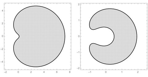
Figure 5. The domain $\Sigma_{s}$ with $s=3$ (left) and the domain $\Sigma_{s,t}$ with $s=3$, $t=1$ (right). The map $f_{s-t}=f_{2}$ takes the complement of the domain on the left to the complement of the domain on the right

We need a two-parameter version of Proposition 2.3. To formulate the correct generalization, we first note that the function $f_{s}$ satisfies

$$f_{s}(0)=0;\quad f_{s}^{\prime}(0)=e^{s/2}\neq 0.$$

Thus, $f_{s}$ has a local inverse defined near zero, which we denote by $\chi_{s}$. Recall from (2.6) that the support of the measure $\nu_{s}$ is a proper arc inside the unit circle for $s<4$ and the whole unit circle for $s\geq 4$.

Proposition 5.1.

For all $s>0$, $\chi_{s}$ can be extended uniquely to a holomorphic function on $\mathbb{C}\setminus\mathrm{supp}\,\nu_{s}$ satisfying

$$\chi_{s}(1/z)=1/\chi_{s}(z).$$ (5.4)

Note that when $s\geq 4$, the support of $\nu_{s}$ is the entire unit circle, in which case $\mathbb{C}\setminus\mathrm{supp}\,\nu_{s}$ is a disconnected set. For such values of $s$, the proposition is really asserting just that $\chi_{s}$ extends from a neighborhood of the origin to the open unit disk, at which point (5.4) serves to define $\chi_{s}(z)$ for $\left|z\right|>1$.

For $s>t/2$, define a function $\chi_{s,t}$ by

$$\chi_{s,t}=f_{s-t}\circ\chi_{s}.$$ (5.5)

Since $\chi_{s}$ maps $\mathbb{C}\setminus\mathrm{supp}\,\nu_{s}$ holomorphically to a region that does not include 1, we see that $\chi_{s,t}$ can also be defined holomorphically on $\mathbb{C}\setminus\mathrm{supp}\,\nu_{s}$. Ho established the following result, generalizing Proposition 2.3. (See [29, Section 4.2], including the discussion following Remark 4.7.)

Proposition 5.2.

For all positive numbers $s$ and $t$ with $s>t/2$, define $\Sigma_{s,t}$ by (5.3). Then the function $\chi_{s,t}$ maps $\mathbb{C}\setminus\mathrm{supp}(\nu_{s})$ injectively onto the complement of $\overline{\Sigma}_{s,t}$. We denote the inverse function by $f_{s,t}$, so that

$$f_{s,t}\colon\mathbb{C}\setminus\overline{\Sigma}_{s,t}\rightarrow\mathbb{C}\setminus\mathrm{supp}\,\nu_{s}.$$

Note that, at least for sufficiently small $z$, we have $f_{s,t}(z)=f_{s}(\chi_{s-t}(z))$, by taking inverses in (5.5).

5.4. The main result

We are now ready to state the two-parameter version of Theorem 1.1.

Theorem 5.3.

Let $b_{s,t}$ be the free multiplicative Brownian motion with parameters $(s,t)$, as in (5.2). Then the support of the Brown measure $\mu_{b_{s,t}}$ is contained in $\overline{\Sigma}_{s,t}$.

As in the one-parameter case, we expect that the limiting empirical eigenvalue distribution for $B_{s,t}^{N}:=B_{s,t}^{N}(1)$ will also be supported in $\Sigma_{s,t}$. This is supported by simulations; see Figure 6. More generally, we expect that the empirical eigenvalue distribution of the Brownian motion $B_{s,t}^{N}$ in $\mathrm{GL}(N;\mathbb{C})$ will converge almost surely to $\mu_{b_{s,t}}$ as $N\rightarrow\infty$. This question will be explored in a future paper.

Remark 5.4.

While they do not determine the Brown measure, it is worth noting that the values of the holomorphic moments of $b_{s,t}$ were computed in [30]:

$$\tau(b_{s,t}^{n})=\nu_{n}(s-t)$$ (5.6)

for all $n\in\mathbb{Z}$ and all $s>t/2>0$; here $\nu_{n}(r)$ are the moments of $u_{r}$, cf. (2.5). In particular, when $s=t$, since $\nu_{n}(0)=1$ for all $n$, this recovers the fact that all holomorphic moments of $b_{t}$ are $1$.

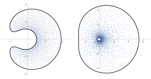
Figure 6. Simulations of the Brownian motions $B_{s,t}^{N}$ for $N=2000$ and $(s,t)=(3,1)$ (left) and $(s,t)=(5,3)$ (right), plotted against the domains $\Sigma_{s,t}$

Remark 5.5.

Now having fully defined the two-paramer Brownian motion and associated notation, we show how to connect the formulas in the physics papers [36, 32] to our formulas. In [36], the boundary of the domain is given by Eq. (83), which is easily seen to be equivalent to our condition for the boundary of $\Sigma_{t},$ namely $\left|f_{t}(\lambda)\right|=1$ with $\left|\lambda\right|\neq 1.$ In [32], the boundary of the domain in the one-parameter case is given by Eq. (5.31), which agrees with Eq. (83) in [36]. In [32], meanwhile, the boundary of the domain in the two-parameter case is given by Eq. (6.37), which is equivalent to saying that their variable $\hat{z}$ should belong to the boundary of the domain $\Sigma_{t_{+}}.$ Meanwhile, using Eqs. (6.30) and (6.36) and a bit of algebra, we find that $\hat{z}$ is related to $z$ by the equation

$$z=f_{t_{-}}(\hat{z}).$$

We conclude that the boundary of their domain is computed as $f_{t_{-}}(\partial\Sigma_{t_{+}}).$ This agrees with the boundary of our domain $\Sigma_{s,t}$, provided we identify their parameters $t_{+}$ and $t_{-}$ with our $s$ and $s-t,$ respectively.

6. Proofs

In this final section, we present the complete proof of Theorem 5.3, which includes the main Theorem 1.1 as the special case $s=t$. We follow the outline of Section 4, and will therefore provide proofs of Theorem 4.1 and (a two-parameter generalization of) Theorem 4.2. We begin with the former.

6.1. A general result on the support of the Brown measure

In this subsection, we work with a general operator in a tracial von Neumann algebra $(\mathcal{A},\tau)$.

For $1\leq p<\infty$, the noncommutative $L^{p}$ norm on $\mathcal{A}$ is

$$\left\|a\right\|_{p}=(\tau[\left|a\right|^{p}])^{1/p}.$$

The noncommutative $L^{p}$ space $L^{p}(\mathcal{A},\tau)$ is the completion of $\mathcal{A}$ with respect to this norm; it can be concretely realized as a space of (largely unbounded, densely-defined) operators affiliated to $\mathcal{A}$.

For $a,b\in\mathcal{A}$ we have the inequality

$$\left\|ab\right\|_{p}\leq\left\|a\right\|\left\|b\right\|_{p}.$$

This shows that the operation of “left multiplication by $a$” is bounded as an operator on $\mathcal{A}$ with respect to the noncommutative $L^{p}$ norm. Thus, by the bounded linear transformation theorem (e.g. [37, Theorem I.7]), left multiplication by $a$ extends uniquely to a bounded linear map (with the same norm) of $L^{p}(\mathcal{A},\tau)$ to itself. We may easily verify that

$$(ab)c=a(bc)$$ (6.1)

for $a,b\in\mathcal{A}$ and $c\in L^{p}(\mathcal{A},\tau)$; this result holds when $c\in\mathcal{A}$ and then extends by continuity. Similar results hold for right multiplication by $a.$

Similarly, since

$$\left\|ab\right\|_{1}\leq\left\|a\right\|_{2}\left\|b\right\|_{2},$$ (6.2)

for all $a,b\in\mathcal{A},$ the product map $(a,b)\mapsto ab$ can be extended by continuity first in $a$ and then in $b,$ giving a map from $L^{2}(\mathcal{A},\tau)\times L^{2}(\mathcal{A},\tau)\rightarrow L^{1}(\mathcal{A},\tau)$ satisfying (6.2). We then observe a simple “associativity” property for the actions of $\mathcal{A}$ on $L^{1}$ and $L^{2}$:

$$a(bc)=(ab)c;\quad(bc)a=b(ca).$$ (6.3)

For any $1\leq p<\infty$, we say that an element $a\in\mathcal{A}$ has an inverse in $L^{p}$ if there is an element $b$ of the noncommutative $L^{p}$ space $L^{p}(\mathcal{A},\tau)$ such that $ab=ba=1$.

Definition 6.1.

Let $a\in\mathcal{A}$, $n\in\mathbb{N}$, and $p\geq 1$. We say that $\lambda_{0}$ belongs to the $L_{n}^{p}$-resolvent set of $a$ if $(a-\lambda)^{n}$ has an inverse, denoted $(a-\lambda)^{-n}$, in $L^{p}$ for all $\lambda$ in a neighborhood of $\lambda_{0}$ and $\left\|(a-\lambda)^{-n}\right\|_{L^{p}}$ is bounded near $\lambda_{0}$. We say that $\lambda_{0}$ is in the $L_{n}^{p}$-spectrum of $a$ if $\lambda_{0}$ is not in the $L_{n}^{p}$-resolvent set of $a$. We denote the $L_{n}^{p}$-spectrum of $a$ by $\mathrm{spec}_{n}^{p}(a)$.

Note that if $a-\lambda_{0}$ has a bounded inverse, then so does $a-\lambda$ for all $\lambda$ sufficiently near $\lambda_{0}$, and $\left\|(a-\lambda)^{-1}\right\|_{\mathcal{A}}$—and therefore $\left\|(a-\lambda)^{-n}\right\|_{\mathcal{A}}$—is automatically bounded near $\lambda_{0}$. It follows that any point in the ordinary resolvent set of $a$ is also in the $L_{n}^{p}$-resolvent set; equivalently,

$$\mathrm{spec}_{n}^{p}(a)\subset\mathrm{spec}(a),$$

where $\mathrm{spec}(a)$ is the ordinary spectrum of $a$. Theorem 4.1 may then be restated as follows, strengthening the standard result that the Brown measure is supported on $\mathrm{spec}(a)$.

Theorem 6.2.

The support of the Brown measure $\mu_{a}$ of $a$ is contained in $\mathrm{spec}_{2}^{2}(a)$.

The concept of “$L^{2}$ spectrum” has come up in prior literature, most notably in the previously mentioned paper [22] of Haagerup and Larsen on the Brown measures of $\mathscr{R}$-diagonal operators. As noted at the end of Section 2.3, if $a$ is $\mathscr{R}$-diagonal, its Brown measure is rotationally invariant. What is more, Haagerup and Larsen show (1) that the support of the Brown measure of $a$ is the closed disk of radius of $\|a\|_{2}$, if $a$ does not have an inverse in $L^{2}$, and (2) that the support of the Brown measure of $a$ is the closed annulus with inner radius $1/\|a^{-1}\|_{2}$ and outer radius $\|a\|_{2}$, if $a$ does have an inverse in $L^{2}$.

Thus, in the notation introduced above, for an $\mathscr{R}$-diagonal element $a$, the point $0$ belongs to the support of the Brown measure if and only if 0 is in the $L^{2}_{1}$-spectrum of $a$. It is, at first, surprising that Haagerup and Larsen’s result is for the $L^{2}_{1}$-spectrum, whereas Theorem 6.2 is for the $L^{2}_{2}$-spectrum. There is, however, a simple explanation for this apparent discrepancy. In the case that $a$ is $\mathscr{R}$-diagonal, the restricted form of the free cumulants (cf. [35, Lecture 15]) implies that $\|a^{-2}\|_{2}=\|a^{-1}\|_{2}^{2}$; hence $0\in\mathrm{spec}^{2}_{1}(a)$ if and only if $0\in\mathrm{spec}_{2}^{2}(a)$.

Thus, our condition in Theorem 6.2 is closely related to the one in [22]. Indeed, Theorem 6.2 can be thought of as an extension of the line of reasoning in [22] to general, non-$\mathscr{R}$-diagonal operators.

It is natural to wonder, from the above definitions, how far the $L^{p}_{n}$-spectra of an operator may differ from each other, and from the actual spectrum. To this end, Haagerup and Larsen give examples where $\mathrm{spec}_{1}^{2}(a)\neq\mathrm{spec}(a)$. Let $h$ be a positive semi-definite operator that is not invertible in $\mathcal{A}$ but is invertible in $L^{2}(\mathcal{A},\tau)$ (i.e. its distribution $\mu_{h}$ has mass in every neighborhood of $0$, but $\int x^{-2}\mu_{h}(dx)<\infty$). If $u$ is a Haar unitary operator freely independent from $h$, then $a=uh$ is an $\mathscr{R}$-diagonal operator for which $a^{-1}\in L^{2}(\mathcal{A},\tau)\setminus\mathcal{A}$; in other words $0\in\mathrm{spec}(a)\setminus\mathrm{spec}_{1}^{2}(a)$, so $\mathrm{spec}_{1}^{2}(a)\subsetneq\mathrm{spec}(a)$. What’s more, in this case, $\mathrm{spec}(a)$ is the full closed disk of radius $\|a\|_{2}$, while $\mathrm{spec}_{1}^{2}(a)$ is the afore-mentioned annulus, cf. [22, Proposition 4.6]. Hence, the support of the Brown measure, and more generally the sets $\mathrm{spec}_{n}^{p}(a)$, may be substantially smaller than the spectrum of $a$.

To prove Theorem 6.2, we need is the following.

Proposition 6.3.

Suppose $a\in\mathcal{A}$ and $a^{2}$ has an inverse, denoted $a^{-2}$, in $L^{2}(\mathcal{A},\tau)$. Then for all $\varepsilon>0$, we have

$$\tau[(a^{\ast}a+\varepsilon)^{-1}(aa^{\ast}+\varepsilon)^{-1}]\leq\left\|a^{-2}\right\|_{L^{2}(\mathcal{A},\tau)}^{2}.$$ (6.4)

Theorem 6.2 follows immediately from Proposition 6.3 together with Corollary 2.6. To prove the proposition, we need the following lemmas.

Lemma 6.4.

For $a,b\in\mathcal{A},$ if $a$ is invertible in $\mathcal{A}$ and $b$ is invertible in $L^{p},$ then $ab$ and $ba$ are invertible in $L^{p}$ with inverses $b^{-1}a^{-1}$ and $a^{-1}b^{-1},$ respectively. If $a$ and $b$ are invertible in $L^{2}$ then $ab$ is invertible in $L^{1}$ with inverse $b^{-1}a^{-1}.$ Finally, if $a$ is invertible in $L^{p}$ then $a^{\ast}$ is invertible in $L^{p}$ with inverse $(a^{-1})^{\ast}.$

Proof.

For $a,b\in\mathcal{A}$ with $b$ invertible in $L^{p},$ we have

$$b^{-1}a^{-1}(ab) =((b^{-1}a^{-1})a)b=((b^{-1}(a^{-1}a))b$$

$$=b^{-1}b=1,$$

where we have used (6.1) twice, and similarly for the product in the other order. A similar argument, using both (6.1) and (6.3), verifies the second claim. Finally, the identity $(ab)^{\ast}=b^{\ast}a^{\ast}$, which holds initially for $a,b\in\mathcal{A}$, extends by continuity to the case $a\in\mathcal{A},$ $b\in L^{p}(\mathcal{A},\tau).$ Thus, if $a$ is invertible in $L^{p},$ then $a^{\ast}(a^{-1})^{\ast}=(a^{-1}a)^{\ast}=1$ and similarly for the product in the reverse order. ∎

Lemma 6.5.

Let $x$ be a non-negative element of $\mathcal{A}$ and suppose $x$ has an inverse in $L^{1}$. Then

$$\lim_{\varepsilon\rightarrow 0^{+}}\tau[(x+\varepsilon)^{-1}]=\tau[x^{-1}].$$

Proof.

We begin by noting that

$$x^{-1}-(x+\varepsilon)^{-1} =x^{-1}((x+\varepsilon)-x)(x+\varepsilon)^{-1}$$

$$=\varepsilon x^{-1}(x+\varepsilon)^{-1}.$$

Now, $\|(x+\varepsilon)^{-1}\|$ is at most $1/\varepsilon$, by the equality of norm and spectral radius for self-adjoint elements. Thus,

$$\|x^{-1}-(x+\varepsilon)^{-1}\|_{1}\leq\varepsilon\|(x+\varepsilon)^{-1}\|\|x^{-1}\|_{1}\leq\|x^{-1}\|_{1}.$$

It follows that $\|(x+\varepsilon)^{-1}\|_{1}\leq 2\|x^{-1}\|_{1}$ for all $\varepsilon>0$.

Let $E^{x}$ be the projection-valued measure associated to $x$ by the spectral theorem. Then

$$\|(x+\varepsilon)^{-1}\|_{1}=\int_{0}^{\infty}\frac{1}{\lambda+\varepsilon}\,\tau[E^{x}(d\lambda)]\leq 2\|x^{-1}\|_{1}.$$

Thus, by monotone convergence, we have

$$\int_{0}^{\infty}\frac{1}{\lambda}\,\tau[E^{x}(d\lambda)]\leq 2\|x^{-1}\|_{1}<\infty.$$

Once this is established, we note that for $\lambda>0$,

$$\left|\frac{1}{\lambda}-\frac{1}{\lambda+\varepsilon}\right|=\frac{\varepsilon}{\lambda(\lambda+\varepsilon)}\leq\frac{1}{\lambda}.$$

Thus, by dominated convergence, $1/(\lambda+\varepsilon)$ converges in $L^{1}((0,\infty),\tau\circ E^{x})$ to $1/\lambda$ as $\varepsilon\rightarrow 0$. It follows that for any sequence $\{\varepsilon_{n}\}$ tending to zero, the operators $(x+\varepsilon_{n})^{-1}$ form a Cauchy sequence with respect to the noncommutative $L^{1}$ norm. Since, by dominated convergence, the functions $\lambda/(\lambda+\varepsilon_{n})$ converge to 1 in $L^{1}((0,\infty),\tau\circ E^{x})$, we can easily see that the limit of $(x+\varepsilon_{n})^{-1}$ in the Banach space $L^{1}(\mathcal{A},\tau)$ is the inverse in $L^{1}$ of $x$.

We have shown, then, that the (unique) inverse in $L^{1}$ of $x$ is the limit in $L^{1}$ of $(x+\varepsilon_{n})^{-1}$. Applying $\tau$ to this result gives the claim, along any sequence $\{\varepsilon_{n}\}$ tending to zero. ∎

Lemma 6.6.

Let $x,y\geq 0$ be positive semidefinite operators in $\mathcal{A}$, and suppose that they are invertible in $L^{1}(\mathcal{A},\tau)$. If $x\leq y$ (i.e., $x-y$ is positive semidefinite) then $\tau(y^{-1})\leq\tau(x^{-1})$.

Proof.

For all $\varepsilon>0$, the elements $x+\varepsilon$ and $y+\varepsilon$ are invertible in $\mathcal{A}$ and $x+\varepsilon\geq y+\varepsilon$. Thus, by the (reverse) operator monotonicity of the inverse [3, Prop. V.1.6], we have

$$\tau((y+\varepsilon)^{-1})\geq\tau((x+\varepsilon)^{-1}).$$ (6.5)

By Lemma 6.5, the claimed result then follows. ∎

Lemma 6.7.

Let $a\in\mathcal{A}$ and suppose that $a^{2}$ has an inverse in $L^{2}(\mathcal{A},\tau)$. Then $a$ and $a^{\ast}$ have inverses in $L^{2}$; and hence $a^{\ast}a$ and $aa^{\ast}$ have inverses in $L^{1}(\mathcal{A},\tau)$.

Proof.

Let $b=a^{-2}$ denote the $L^{2}(\mathcal{A},\tau)$ inverse of $a^{2}$. First, note that $a(ab)=a^{2}b=1$ and $(ba)a=ba^{2}=1$. Since $ab$ and $ba$ are in $L^{2}(\mathcal{A},\tau)$, it follows that $a$ is both left and right invertible in $L^{2}(\mathcal{A},\tau)$. Hence, $a$ is invertible in $L^{2}(\mathcal{A},\tau)$, by the usual argument and (6.1). Taking adjoints shows that $a^{\ast}$ is also invertible in $L^{2}(\mathcal{A},\tau)$. Thus $aa^{\ast}[(a^{\ast})^{-1}a^{-1}]=1=[(a^{\ast})^{-1}a^{-1}]aa^{\ast}$. Since $(a^{\ast})^{-1}$ and $a^{-1}$ are in $L^{2}(\mathcal{A},\tau)$, their product is in $L^{1}(\mathcal{A},\tau)$ by Hölder’s inequality; this shows $aa^{\ast}$ is invertible in $L^{1}(\mathcal{A},\tau)$. An analogous argument holds for $a^{\ast}a$. ∎

We are now ready for the proof of Proposition 6.3.

Proof of Proposition 6.3.

We begin by arguing formally and then fill in the details. We start by noting that

$$(a^{\ast}a+\varepsilon)^{1/2}(aa^{\ast}+\varepsilon)(a^{\ast}a+\varepsilon)^{1/2}-(a^{\ast}a+\varepsilon)^{1/2}(aa^{\ast})(a^{\ast}a+\varepsilon)^{1/2} =\varepsilon(a^{\ast}a+\varepsilon)$$

$$\geq 0.$$

Thus, by Lemma 6.4 and the cyclic property of the trace, we have

$$\tau[(a^{\ast}a+\varepsilon)^{-1}(aa^{\ast}+\varepsilon)^{-1}] =\tau[(a^{\ast}a+\varepsilon)^{-1/2}(aa^{\ast}+\varepsilon)^{-1}(a^{\ast}a+\varepsilon)^{-1/2}]$$

$$\leq\tau[(a^{\ast}a+\varepsilon)^{-1/2}(aa^{\ast})^{-1}(a^{\ast}a+\varepsilon)^{-1/2}]$$

$$=\tau[(aa^{\ast})^{-1}(a^{\ast}a+\varepsilon)^{-1}].$$ (6.6)

We then use the same argument again. We note that

$$a^{\ast}(a^{\ast}a+\varepsilon)a-a^{\ast}(a^{\ast}a)a=\varepsilon a^{\ast}a\geq 0,$$ (6.7)

from which we obtain

$$\tau[(aa^{\ast})^{-1}(a^{\ast}a+\varepsilon)^{-1}] =\tau[a^{-1}(a^{\ast}a+\varepsilon)^{-1}(a^{\ast})^{-1}]$$

$$=\tau[(a^{\ast}(a^{\ast}a+\varepsilon)a)^{-1}]$$

$$\leq\tau[((a^{\ast})^{2}a^{2})^{-1}]$$

$$=\tau[a^{-2}(a^{-2})^{\ast}].$$

$$=\left\|a^{-2}\right\|_{L^{2}(\mathcal{A},\tau)}^{2}$$ (6.8)

Combining (6.6) and (6.8) gives the desired inequality.

To make the argument rigorous, we need to make sure that all the relevant inverses exist in $L^{1}(\mathcal{A},\tau),$ so that Lemma 6.4 is applicable. The operator $(a^{\ast}a+\varepsilon)^{1/2}(aa^{\ast}+\varepsilon)(a^{\ast}a+\varepsilon)^{1/2}$ is invertible in $\mathcal{A}$ and thus in $L^{1}(\mathcal{A},\tau).$ On the other hand, by assumption $a^{2}$ is invertible in $L^{2}(\mathcal{A},\tau)$. It then follows from Lemma 6.5 that $aa^{\ast}$ is invertible in $L^{1}(\mathcal{A},\tau),$ so that $(a^{\ast}a+\varepsilon)^{1/2}(aa^{\ast})(a^{\ast}a+\varepsilon)^{1/2}$ is also invertible in $L^{1}(\mathcal{A},\tau),$ by Lemma 6.4. Thus, Lemma 6.4 is applicable in (6.6).

We now consider the two terms on the left-hand side of (6.7). By Lemma 6.5, both $a$ and $a^{\ast}$ are invertible in $L^{2}$; it then follows from Lemma 6.4 that $a^{\ast}(a^{\ast}a+\varepsilon)$ is invertible in $L^{2}$ and that $a^{\ast}(a^{\ast}a+\varepsilon)a$ is invertible in $L^{1}.$ Meanwhile, $a^{2}$ is, by assumption, invertible in $L^{2}$; it then follows from Lemma 6.4 that $(a^{\ast})^{2}$ is invertible in $L^{2}.$ Thus, using Lemma 6.4 one last time, we conclude that $(a^{\ast})^{2}a^{2}$ is invertible in $L^{1}.$ Thus, Lemma 6.5 is also applicable in (6.8). ∎

6.2. Computing the $L_{2}^{2}$ spectrum

We consider the free multiplicative $(s,t)$ Brownian motion $b_{s,t}$ defined in (5.2) as an element of a tracial von Neumann algebra $(\mathcal{B},\tau)$. Recall that when $s=t$, the operator $b_{s,t}$ has the same noncommutative distribution as the ordinary free multiplicative Brownian motion $b_{t}$ described in Section 2.1. Our goal is to prove a two-parameter version of Theorem 4.2 from Section 4, by constructing an $L^{2}$ inverse to $(b_{s,t}-\lambda)^{n}$ for $\lambda$ in the complement of $\overline{\Sigma}_{s,t}$, with local bounds on the norm of the inverse. This will, in particular, show that

$$\mathrm{spec}_{n}^{2}(b_{s,t})\subset\overline{\Sigma}_{s,t}$$ (6.9)

for all $n$. (Recall Definition 6.1.) If we specialize (6.9) to the case $n=2$, Theorem 6.2 will then tell us that the support of the Brown measure of $b_{s,t}$ is contained in $\overline{\Sigma}_{s,t}$.

Our tool is the two-parameter “free Hall transform” $\mathscr{G}_{s,t}$ (cf. Section 5), which includes the one-parameter transform $\mathscr{G}_{t}=\mathscr{G}_{t,t}$ (cf. Section 3) as a special case. To avoid technical issues for the case $s=4$, we introduce a variant of the transform $\mathscr{G}_{s,t}$, denoted $\mathscr{S}_{s,t}$. Define

$$L_{\mathrm{hol}}^{2}(b_{s,t},\tau)$$

to be the closure in the noncommutative $L^{2}$ norm of the space of elements of the form $p(b_{s,t})$, where $p$ is a Laurent polynomial in one variable.

If $\mathcal{P}$ denotes the space of Laurent polynomials in one variable, then [14, Theorem 1.13] shows that $\mathscr{G}_{s,t}$ maps $\mathcal{P}$ bijectively onto $\mathcal{P}$. We then define $\mathscr{S}_{s,t}$ initially on $\mathcal{P}$ by evaluating each polynomial $\mathscr{G}_{s,t}(p)$ on the element $b_{s,t}$:

$$\mathscr{S}_{s,t}(p)=\mathscr{G}_{s,t}(p)(b_{s,t})\in L_{\mathrm{hol}}^{2}(b_{s,t},\tau).$$

By [29, Theorem 5.7], $\mathscr{S}_{s,t}$ maps $\mathcal{P}\subset L^{2}(\partial\mathbb{D},\nu_{s})$ isometrically into $L_{\mathrm{hol}}^{2}(b_{s,t},\tau)$. (Although some parts of the just-cited theorem implicitly assume that $s\neq 4$, Part 2 of the theorem does not depend on this assumption.) Furthermore, since $\mathscr{G}_{s,t}$ maps onto $\mathcal{P}$, the image of $\mathscr{S}_{s,t}$ is dense in $L_{\mathrm{hol}}^{2}(b_{s,t},\tau)$. Thus, $\mathscr{S}_{s,t}$ extends to a unitary map

$$\mathscr{S}_{s,t}:L^{2}(\partial\mathbb{D},\nu_{s})\rightarrow L_{\mathrm{hol}}^{2}(b_{s,t},\tau).$$

For $\lambda\in\mathbb{C}\setminus\overline{\Sigma}_{s,t}$, we will then construct an inverse $(b_{s,t}-\lambda)^{-n}$ to $(b_{s,t}-\lambda)^{n}$ in $L_{\mathrm{hol}}^{2}(b_{s,t},\tau)$ by constructing the preimage of $(b_{s,t}-\lambda)^{-n}$ under $\mathscr{S}_{s,t}$. Note that in Section 4, we outlined the proof in the case $s=t$, with $t\neq 4$. In that case, [5, Lemma 17] allows us to identify $L_{\mathrm{hol}}^{2}(\mathcal{B},\tau)$ with the space $\mathscr{A}_{t}$, in which case, it is harmless to work with $\mathscr{G}_{s,t}$ instead of $\mathscr{S}_{s,t}$.

Recall the definition of the function $f_{s,t}$ in Proposition 5.2.

Theorem 6.8.

Define a function $r_{\lambda}^{s,t}\in L^{2}(\partial\mathbb{D},\nu_{s})$ by the formula

$$r_{\lambda}^{s,t}(\omega)=\frac{f_{s,t}(\lambda)}{\lambda}\left(\frac{1}{\omega-f_{s,t}(\lambda)}\right),\quad\omega\in\mathrm{supp}(\nu_{s}),$$ (6.10)

for all $\lambda\in\mathbb{C}\setminus\overline{\Sigma}_{s,t}$. Then for all such $\lambda$, we have

$$\mathscr{S}_{s,t}(r_{\lambda}^{s,t})=(b_{s,t}-\lambda)^{-1}.$$

That is to say, $\mathscr{S}_{s,t}(r_{\lambda}^{s,t})$ is an inverse in $L^{2}$ of $(b_{s,t}-\lambda)$.

Recall from Proposition 5.2 that $f_{s,t}(\lambda)$ is outside the support of $\nu_{s}$ for all $\lambda$ in the complement of $\overline{\Sigma}_{s,t}$. Thus, $r_{\lambda}^{s,t}(\omega)$ is bounded and is therefore a $\nu_{s}$–square integrable function of $\omega$ for all $\lambda\in\mathbb{C}\setminus\overline{\Sigma}_{s,t}$.

When $\lambda=0$, we interpret $r_{\lambda}^{s,t}$ to be the limit of the right-hand side of (6.10) as $\lambda$ approaches zero, which is easily computed to be $r_{0}^{s,t}(\omega)=e^{t/2}\omega^{-1}$.

Proof.

For the case $\lambda=0$, we compute that $\mathscr{G}_{s,t}(\omega^{-1})=e^{-t/2}z^{-1}$, as may be verified from the behavior of $\mathscr{G}_{s,t}$ with respect to inversion [14, Eq. (5.2)] and the recursive formula in [14, Proposition 5.2]. Thus, by definition, we have $\mathscr{S}_{s,t}(\omega^{-1})=e^{-t/2}b_{s,t}^{-1}$ so that $\mathscr{S}_{s,t}(e^{t/2}\omega^{-1})=b_{s,t}^{-1}$, which is the $\lambda=0$ case of the theorem. The subsequent calculations assume $\lambda\neq 0$.

We start by considering large values of $\lambda$. For $\left|\lambda\right|>\left\|b_{s,t}\right\|$, the element $b_{s,t}-\lambda$ has a bounded inverse, which may be computed as a power series:

$$(b_{s,t}-\lambda)^{-1}=-\frac{1}{\lambda}(1-b_{s,t}/\lambda)^{-1}=-\frac{1}{\lambda}\sum_{k=0}^{\infty}\lambda^{-k}(b_{s,t})^{k},$$

with the series converging in the operator norm and thus also in the noncommutative $L^{2}$ norm. Applying $\mathscr{S}_{s,t}^{-1}$ term by term gives

$$\mathscr{S}_{s,t}^{-1}\left((b_{s,t}-\lambda)^{-1}\right)(\omega) =-\frac{1}{\lambda}\sum_{k=0}^{\infty}\lambda^{-k}p_{k}^{s,t}(\omega)$$ (6.11)

$$=-\frac{1}{\lambda}\left[1+\Pi(s,t,\omega,1/\lambda)\right],$$ (6.12)

where $p_{k}^{s,t}$ is the unique polynomial such that

$$\mathscr{G}_{s,t}(p_{k}^{s,t})(z)=z^{k},\quad k\in\mathbb{Z},$$

and where $\Pi$ is the generating function in [14, Theorem 1.17].

Meanwhile, according to [14, Eq. (1.21)], we have the following implicit formula for $\Pi$:

$$\Pi(s,t,\omega,f_{s-t}(z))=\frac{1}{1-\omega f_{s}(z)}-1.$$

(This result extends a formula of Biane in the $s=t$ case.) Then, at least for sufficiently small $z$, we may replace $z$ by $\chi_{s-t}(z)$, where $\chi_{s,t}$ is the inverse function to $f_{s-t}$. This substitution gives

$$\Pi(s,t,\omega,z)=\frac{1}{1-\omega f_{s}(\chi_{s-t}(z))}-1.$$ (6.13)

Plugging this expression into (6.12) gives

$$r_{\lambda}^{s,t}(\omega)=-\frac{1}{\lambda}\frac{1}{1-\omega f_{s}(\chi_{s-t}(1/\lambda))},$$

for $\lambda$ sufficiently large, which simplifies—using (5.4) and the identity $f_{s}(1/z)=1/f_{s}(z)$—to the expression in (6.10).

Similarly, for $0<\left|\lambda\right|<1/\left\|b_{s,t}^{-1}\right\|$, we use the series expansion

$$(b_{s,t}-\lambda)^{-1} =b_{s,t}^{-1}(1-\lambda b_{s,t}^{-1})^{-1}$$

$$=b_{s,t}^{-1}\sum_{k=0}^{\infty}\lambda^{k}b_{s,t}^{-k}$$

$$=\frac{1}{\lambda}\sum_{k=1}^{\infty}\lambda^{k}b_{s,t}^{-k}.$$

Since $p_{-k}^{s,t}(\omega)=p_{k}^{s,t}(\omega^{-1})$ (see [14, Eq. (5.2)]), we may apply $\mathscr{S}_{s,t}^{-1}$ term by term to obtain

$$\mathscr{S}_{s,t}^{-1}\left((b_{s,t}-\lambda)^{-1}\right)(\omega) =\frac{1}{\lambda}\sum_{k=1}^{\infty}\lambda^{k}p_{k}^{s,t}(\omega^{-1})$$

$$=\frac{1}{\lambda}\Pi(s,t,\omega^{-1},\lambda).$$

Using the formula (6.13) for $\Pi$ (for sufficiently small $\lambda$) and simplifying gives the same expression as for the large-$\lambda$ case.

Finally, for general $\lambda\in\mathbb{C}\setminus\overline{\Sigma}_{s,t}$ we use an analytic continuation argument. The complement of the closure of $\Sigma_{s,t}$ has at most two connected components, the unbounded component and, for $s\geq 4$, a bounded component containing 0. Now, for all $\lambda\in\mathbb{C}\setminus\overline{\Sigma}_{s,t}$, the function $r_{\lambda}^{s,t}$ in (6.10) is a well-defined element of $L^{2}(\partial\mathbb{D},\nu_{s})$, because (by Proposition 5.2) $f_{s,t}$ maps $\mathbb{C}\setminus\overline{\Sigma}_{s,t}$ into $\mathbb{C}\setminus\mathrm{supp}\,\nu_{s}$. Furthermore, it is evident from (6.10) that $r_{\lambda}^{s,t}$ is a weakly holomorphic function of $\lambda\in\mathbb{C}\setminus\overline{\Sigma}_{s,t}$, with values in $L^{2}(\partial\mathbb{D},\nu_{s})$, meaning that $\lambda\mapsto\phi(r_{\lambda}^{s,t})$ is a holomorphic for each bounded linear functional on $L^{2}(\partial\mathbb{D},\nu_{s})$.

Thus, since $\mathscr{S}_{s,t}$ is unitary (hence bounded), $\mathscr{S}_{s,t}(r_{\lambda}^{s,t})$ is a weakly holomorphic function of $\lambda\in\mathbb{C}\setminus\overline{\Sigma}_{s,t}$, with values in $L_{\mathrm{hol}}^{2}(\mathcal{B},\tau)$. It is then easy to see that

$$(b_{s,t}-\lambda)\mathscr{S}_{s,t}(r_{\lambda}^{s,t})=b_{s,t}\mathscr{S}_{s,t}(r_{\lambda}^{s,t})-\lambda\mathscr{S}_{s,t}(r_{\lambda}^{s,t})$$ (6.14)

is also weakly holomorphic. After all, applying a bounded linear functional $\phi$ gives

$$\phi(b_{s,t}\mathscr{S}_{s,t}(r_{\lambda}^{s,t}))-\lambda\phi(\mathscr{S}_{s,t}(r_{\lambda}^{s,t})).$$ (6.15)

Since multiplication by $b_{s,t}$ is a bounded linear map on $L_{\mathrm{hol}}^{2}(\mathcal{B},\tau)$, the linear functional $\phi(b_{s,t}\cdot)$ is bounded, so both terms in (6.15) are holomorphic in $\lambda$.

Meanwhile, we have shown that (6.14) is equal to 1 on a nonempty, open subset of each connected component of $\mathbb{C}\setminus\overline{\Sigma}_{s,t}$. Since, also, (6.14) is weakly holomorphic, it must be equal to 1 on all of $\mathbb{C}\setminus\overline{\Sigma}_{s,t}$. ∎

We emphasize that, although for very large and small $\lambda$ the standard power-series argument gives an inverse of $b_{s,t}-\lambda$ in the algebra $\mathcal{B}$, the analytic continuation takes place in $L_{\mathrm{hol}}^{2}(\mathcal{B},\tau)$, which is the range of the transform $\mathscr{S}_{s,t}$. Thus, for general $\lambda\in\mathbb{C}\setminus\overline{\Sigma}_{s,t}$, we are guaranteed that $b_{s,t}-\lambda$ has an inverse in $L^{2}$, but not necessarily in $\mathcal{B}$.

Corollary 6.9.

For all $\lambda\in\mathbb{C}\setminus\overline{\Sigma}_{s,t}$ and all positive integers $n$, the operator $(b_{s,t}-\lambda)^{n}$ has an inverse $(b_{s,t}-\lambda)^{-n}$ in $L^{2}(\mathcal{B},\tau)$. Specifically,

$$(b_{s,t}-\lambda)^{-n}=\mathscr{S}_{s,t}\left(\frac{1}{(n-1)!}\left(\frac{\partial}{\partial\lambda}\right)^{n-1}r_{\lambda}^{s,t}\right),$$ (6.16)

where $r_{\lambda}^{s,t}$ is as in (6.10). Furthermore, $\left\|(b_{s,t}-\lambda)^{-n}\right\|_{L^{2}(\mathcal{B},\tau)}$ is locally bounded on $\mathbb{C}\setminus\overline{\Sigma}_{s,t}$.

Proof.

We let

$$r_{\lambda}^{s,t,n}(\omega)=\frac{1}{(n-1)!}\left(\frac{\partial}{\partial\lambda}\right)^{n-1}r_{\lambda}^{s,t}(\omega).$$

If we inductively compute the derivatives in the definition of $r_{\lambda}^{s,t,n}(\omega)$, we will find that the result is polynomial in $1/(\omega-f_{s,t}(\lambda))$, with coefficients that are holomorphic functions of $\lambda\in\mathbb{C}\setminus\overline{\Sigma}_{s,t}$. Thus, for each $n$, the quantity $r_{\lambda}^{s,t,n}(\omega)$ is jointly continuous as a function of $\omega\in\mathrm{supp}(\nu_{t})$ and $\lambda\in\mathbb{C}\setminus\overline{\Sigma}_{s,t}$. Thus, $\|r_{\lambda}^{s,t,n}\|_{L^{2}(\partial\mathbb{D},\nu_{s})}$ is finite and depends continuously on $\lambda$. Thus, once (6.16) is verified, the local bounds on the norm of $(b_{s,t}-\lambda)^{-n}$ will follow from the unitarity of $\mathscr{S}_{s,t}$.

We establish (6.16) by induction on $n$, the $n=1$ case being the content of Theorem 6.8. Assume, then, the result for a fixed $n$ and recall that $r_{\lambda}^{s,t,n}(\omega)$ is a polynomial in $1/(\omega-f_{s,t}(\lambda))$, with coefficients that are holomorphic functions of $\lambda$. It is then an elmentary matter to see that for each fixed $\lambda\in\mathbb{C}\setminus\overline{\Sigma}_{s,t}$, the limit

$$\lim_{h\rightarrow 0}\frac{r_{\lambda+h}^{s,t,n}(\omega)-r_{\lambda}^{s,t,n}(\omega)}{h}$$

exists as a uniform limit on $\mathrm{supp}\,\nu_{s}$, and thus also in $L^{2}(\partial\mathbb{D},\nu_{s})$. Applying $\mathscr{S}_{s,t}$ and using our induction hypothesis gives

$$\mathscr{S}_{s,t}\left(\frac{\partial}{\partial\lambda}r_{\lambda}^{s,t,n}(\omega)\right)=\lim_{h\rightarrow 0}\frac{1}{h}[(b_{s,t}-(\lambda+h))^{-n}-(b_{s,t}-\lambda)^{-n}],$$ (6.17)

where the limit is in $L_{\mathrm{hol}}^{2}(b_{s,t},\tau)$.

We now multiply both sides of (6.17) by $(b_{s,t}-\lambda)^{n+1}$, which we write as $(b_{s,t}-\lambda)(b_{s,t}-\lambda)^{n}$. Since multiplication by an element of $\mathcal{B}$ is a continuous linear map on $L^{2}(\mathcal{B},\tau)$, we obtain

$$(b_{s,t}-\lambda)^{n+1}\mathscr{S}_{s,t}\left(\frac{\partial}{\partial\lambda}r_{\lambda}^{s,t,n}(\omega)\right)$$

$$=\lim_{h\rightarrow 0}(b_{s,t}-\lambda)\frac{1}{h}[(b_{s,t}-\lambda)^{n}(b_{s,t}-(\lambda+h))^{-n}-1].$$ (6.18)

In the first term on the right-hand side of (6.18), we write

$$(b_{s,t}-\lambda)^{n}=(b_{s,t}-(\lambda+h)+h)^{n}=\sum_{k=0}^{n}\binom{n}{k}(b_{s,t}-(\lambda+h))^{n-k}h^{k}.$$ (6.19)

Upon substituting (6.19) into (6.18), the $k=0$ term cancels with the existing term of $-1$, while the $k=1$ term gives

$$(b_{s,t}-\lambda)\frac{1}{h}\cdot nh(b_{s,t}-(\lambda+h))^{-1}=n(b_{s,t}-\lambda)(b_{s,t}-(\lambda+h))^{-1}.$$ (6.20)

If we again write $(b_{s,t}-\lambda)=(b_{s,t}-(\lambda+h)+h)$, we see that (6.20) tends to $n\cdot 1$ as $h\to 0$. Finally, all terms with $k\geq 2$ will vanish in the limit, leaving us with

$$(b_{s,t}-\lambda)^{n+1}\mathscr{S}_{s,t}\left(\frac{\partial}{\partial\lambda}r_{\lambda}^{s,t,n}(\omega)\right)=n\cdot 1.$$

Thus,

$$\mathscr{S}_{s,t}\left(\frac{1}{n}\frac{\partial}{\partial\lambda}r_{\lambda}^{s,t,n}(\omega)\right)=(b_{s,t}-\lambda)^{-(n+1)},$$

which is just the level-$(n+1)$ case of the corollary. ∎

Acknowledgments

We would like to thank Adrian Ioana and Ching Wei Ho for useful conversations. We also thank Maciej Nowak for making us aware of the papers [36, 32] and for many illuminating discussions about them. Finally, we thank the anonymous referee for carefully reading our manuscript and, in particular, for suggesting additions that improved the discussion of $L^{p}_{n}$-spectrum.

References

- [1] Z. D. Bai, Circular law, Ann. Probab. 25 (1997), 494–529.
- [2] H. Bercovici and D. Voiculescu, Lévy–Hinčin type theorems for multiplicative and additive free convolution, Pacific J. Math. 153 (1992), 217–248.
- [3] R. Bhatia, Matrix analysis. Graduate Texts in Mathematics, 169. Springer-Verlag, New York, 1997.
- [4] P. Biane, “Free Brownian motion, free stochastic calculus and random matrices.” In Free Probability Theory (Waterloo, ON, 1995), 1–19. Fields Institute Communications 12. Providence, RI: American Mathematical Society, 1997.
- [5] P. Biane, Segal–Bargmann transform, functional calculus on matrix spaces and the theory of semi-circular and circular systems, J. Funct. Anal., 144 (1997), 232–286.
- [6] P. Biane, Processes with free increments, Math. Z. 227 (1998), 143–174.
- [7] P. Biane and R. Speicher, Stochastic calculus with respect to free Brownian motion and analysis on Wigner space, Probab. Theory Related Fields 112 (1998), 373–409.
- [8] P. Biane and R. Speicher, Free diffusions, free entropy and free Fisher information, Ann. Inst. H. Poincaré Probab. Statist. 37 (2001), 581–606.
- [9] B. Blackadar, Operator algebras. Theory of -algebras and von Neumann algebras, Encyclopedia of Mathematical Sciences 122. Operator Algebras and Non-commutative Geometry, III. Springer-Verlag, Berlin, 2006.
- [10] Brown, L. G. Lidskiĭ’s theorem in the type II case. In Geometric methods in operator algebras (Kyoto, 1983), 1–35, Pitman Res. Notes Math. Ser., 123, Longman Sci. Tech., Harlow, 1986.
- [11] G. Cébron, Free convolution operators and free Hall transform, J. Funct. Anal. 265 (2013), 2645–2708.
- [12] B. Collins and T. Kemp, Liberation of projections, J. Funct. Anal. 266 (2014), 1988–2052.
- [13] B. K. Driver and B. C. Hall, Yang–Mills theory and the Segal–Bargmann transform, Comm. Math. Phys. 201 (1999), 249–290.
- [14] B. K. Driver, B. C. Hall, and T. Kemp, The large- limit of the Segal–Bargmann transform on , J. Funct. Anal. 265 (2013), 2585–2644.
- [15] B. K. Driver, B.C. Hall, and T. Kemp, The Brown measure of the free multiplicative Brownian motion, Preprint arXiv:1903.11015
- [16] B. Fuglede and R. V. Kadison, On determinants and a property of the trace in finite factors, Proc. Nat. Acad. Sci. U. S. A. 37 (1951), 425–431.
- [17] B. Fuglede and R. V. Kadison, Determinant theory in finite factors, Ann. of Math. (2) 55 (1952), 520–530.
- [18] J. Ginibre, Statistical ensembles of complex, quaternion, and real matrices, J. Math. Phys. 6 (1965), 440–449.
- [19] V. L. Girko, The circular law. (Russian) Teor. Veroyatnost. i Primenen. 29 (1984), 669–679.
- [20] F. Götze and A. Tikhomirov, The circular law for random matrices, Ann. Probab. 38 (2010), 1444–1491.
- [21] L. Gross and P. Malliavin, Hall’s transform and the Segal–Bargmann map. In Itô’s stochastic calculus and probability theory (N. Ikeda, S. Watanabe, M. Fukushima and H. Kunita, Eds.), 73–116, Springer, 1996.
- [22] U. Haagerup and F. Larsen, Brown’s spectral distribution measure for -diagonal elements in finite von Neumann algebras, J. Funct. Anal. 176 (2000), 331–367.
- [23] B. C. Hall, The Segal–Bargmann “coherent state” transform for compact Lie groups. J. Funct. Anal. 122 (1994), 103–151.
- [24] B. C. Hall, A new form of the Segal–Bargmann transform for Lie groups of compact type, Canad. J. Math. 51 (1999), 816–834.
- [25] B. C. Hall, Harmonic analysis with respect to heat kernel measure, Bull. Amer. Math. Soc. (N.S.) 38 (2001), 43–78.
- [26] B. C. Hall, The Segal–Bargmann transform and the Gross ergodicity theorem. In Finite and infinite dimensional analysis in honor of Leonard Gross (New Orleans, LA, 2001), 99–116, Contemp. Math., 317, Amer. Math. Soc., Providence, RI, 2003.
- [27] B. C. Hall and A. N. Sengupta, The Segal–Bargmann transform for path-groups, J. Funct. Anal. 152 (1998), 220–254.
- [28] B. C. Hall, The Segal–Bargmann transform for unitary groups in the large- limit, preprint arXiv:1308.0615 [math.RT].
- [29] C.-W. Ho, The two-parameter free unitary Segal–Bargmann transform and its Biane–Gross–Malliavin identification, J. Funct. Anal. 271 (2016), 3765–3817.
- [30] T. Kemp, The large- limits of Brownian motions on , Int. Math. Res. Not., (2016), 4012–4057.
- [31] T. Kemp, I. Nourdin, G. Peccati, and R. Speicher, Wigner chaos and the fourth moment. Ann. Prob. 40 (2012), 1577–1635.
- [32] R. Lohmayer, H. Neuberger, and T. Wettig, Possible large-N transitions for complex Wilson loop matrices, J. High Energy Phys. 2008, no. 11, 053, 44 pp.
- [33] H. P. McKean, Stochastic Integrals. Probability and Mathematical Statistics 5. New York: Academic Press, 1969
- [34] J. A. Mingo and R. Speicher, Free probability and random matrices. Fields Institute Monographs, 35. Springer, New York; Fields Institute for Research in Mathematical Sciences, Toronto, ON, 2017.
- [35] A. Nica and R. Speicher, Lectures on the combinatorics of free probability. London Mathematical Society Lecture Note Series, 335. Cambridge University Press, Cambridge, 2006. xvi+417 pp.
- [36] E. Gudowska-Nowak, R. A. Janik, J. Jurkiewicz, and M. A. Nowak, Infinite products of large random matrices and matrix-valued diffusion, Nuclear Phys. B 670 (2003), 479–507.
- [37] M. Reed and B. Simon, Methods of modern mathematical physics. I. Functional analysis. Second edition. Academic Press, Inc. [Harcourt Brace Jovanovich, Publishers], New York, 1980. xv+400 pp.
- [38] I. M. Singer, On the master field in two dimensions. In Functional analysis on the eve of the 21st century, Vol. 1 (New Brunswick, NJ, 1993), volume 131 of Progr. Math., 263–281. Birkhäuser Boston, Boston, MA, 1995.
- [39] T. Tao and V. Vu, Random matrices: universality of ESDs and the circular law. With an appendix by Manjunath Krishnapur. Ann. Probab. 38 (2010), 2023–2065.
- [40] D. V. Voiculescu, Limit laws for random matrices and free products. Invent. Math. 104 (1991), 201–220.