SIGUA: Forgetting May Make Learning with Noisy Labels More Robust

Abstract

Given data with noisy labels, over-parameterized deep networks can gradually memorize the data, and fit everything in the end. Although equipped with corrections for noisy labels, many learning methods in this area still suffer overfitting due to undesired memorization. In this paper, to relieve this issue, we propose stochastic integrated gradient underweighted ascent (SIGUA): in a mini-batch, we adopt gradient descent on good data as usual, and learning-rate-reduced gradient ascent on bad data; the proposal is a versatile approach where data goodness or badness is w.r.t. desired or undesired memorization given a base learning method. Technically, SIGUA pulls optimization back for generalization when their goals conflict with each other; philosophically, SIGUA shows forgetting undesired memorization can reinforce desired memorization. Experiments demonstrate that SIGUA successfully robustifies two typical base learning methods, so that their performance is often significantly improved.

1 Introduction

Data labeling may be heavily noisy in practice where label generation/corruption processes are usually agnostic (Xiao et al., 2015; Jiang et al., 2018; Wang et al., 2019; Welinder et al., 2010). As a result, learning with noisy labels seems inevitable. On the other hand, more complex data requires more expressive power, and then using over-parameterized deep networks as our models seems also inevitable (Goodfellow et al., 2016). This combination of noisy labels and deep networks is very pessimistic, since deep networks are able to fit anything given for training even if the labels are completely random (Zhang et al., 2017). Unfortunately, it is non-trivial to apply general-purpose regularization such as weight decay (Krogh & Hertz, 1991) and dropout (Srivastava et al., 2014) for controlling model complexities of deep networks. General-purpose regularization would hurt the capability of memorizing not only noisy labels but also complex data, which is never our desideratum.

Fortunately, even though deep networks can fit everything in the end, they learn patterns first (Arpit et al., 2017): this suggests deep networks can gradually memorize the data, moving from regular data to irregular data such as outliers and mislabeled data. As a consequence, the memorization events during training may be divided into two categories: desired memorization that helps generalization, and undesired memorization that hurts generalization. Our desideratum is to keep the former and avoid the latter, which may save generalization until the end of training hopefully.

However, it is hard to avoid undesired memorization from the beginning of training, since two categories can be relative to each other and cannot be distinguished without sufficient training. Consider sample selection, a correction for noisy labels where small-loss data are regarded as correct, and deep networks are trained only on selected data (Jiang et al., 2018; Han et al., 2018b; Yu et al., 2019). The losses could be enough informative after enough epochs, but then many mislabeled data have already been memorized many times. Consider backward correction, where the surrogate loss is corrected according to the label corruption process, and deep networks are trained based on this corrected loss (Natarajan et al., 2013; Patrini et al., 2017). The corrected loss is not necessarily a non-negative loss, and it might go fairly negative on a training data, which signifies this data being memorized too much. Thus, these learning methods equipped with corrections for noisy labels still suffer from undesired memorization which in turn leads to overfitting.

To relieve this issue of overfitting due to undesired memorization, we propose stochastic integrated gradient underweighted ascent (SIGUA). Specifically, SIGUA belongs to stochastic optimization and can be integrated into stochastic gradient descent (SGD) or its variants (e.g., Robbins & Monro, 1951; Kingma & Ba, 2015). SIGUA works in each mini-batch: it implements SGD on good data as usual, and if there are any bad data, it implements stochastic gradient ascent (SGA) on bad data with a reduced learning rate. It is a versatile approach, where data goodness or badness is w.r.t. desired or undesired memorization arose in the base learning method. For instance, the good-data condition for sample selection is that the loss of the deep network being trained on a data is relatively small within the mini-batch; that for backward correction is the corrected loss on a data is still positive. We can see that a good-data condition can select desired memorization, and then a bad-data condition should be designed accordingly, so that it can select undesired memorization to be relieved by SGA.

SIGUA can be justified as follows. In machine learning, it is known that optimization shares the goal with generalization in the beginning of training, and we suffer underfitting if optimization is not well done. However, when optimization is well done, its goal will diverge from the goal of generalization, and we suffer overfitting if optimization is too much done. That is why we add regularizations (Goodfellow et al., 2016), including but not limited to the powerful early stopping (Morgan & Bourlard, 1990). Nevertheless, early stopping might not be a good choice, due to the possibility of epoch-wise double descent phenomena occurred in training deep networks (Nakkiran et al., 2020). Hence, we should trade off optimization for generalization without early stopping. Technically, SIGUA is a specially designed regularization by pulling optimization back for generalization when their goals conflict with each other. A key difference between SIGUA and parameter shrinkage like weight decay is that SIGUA pulls optimization back on some data but parameter shrinkage does the same on all data.

Furthermore, it is of vital importance to distinguish desired and undesired memorization in the presence of label noise. Although deep networks are excellent function approximators, they are only good at continuous functions or at least functions without jump discontinuity. However, memorizing mislabeled data asks the deep network being trained to exhibit a certain jump discontinuity, and thus a mislabeled data consumes notably more model capacity than a regular data. In terms of deep learning theory, deep networks have high adaptivity to spatial inhomogeneity of target function smoothness, but a mislabeled data consumes notably more such adaptivity (Suzuki, 2019). Therefore, if the deep network being trained can forget a mislabeled data, an essential amount of model capacity can be returned, which may be properly consumed later. In this sense, philosophically, SIGUA demonstrates that forgetting undesired memorization can reinforce desired memorization, which provides a novel viewpoint on the inductive bias of neural networks.

2 A Prototype of SIGUA

Let $\mathcal{X}$ and $\mathcal{Y}$ be the input and output domains. Consider a $k$-class classification problem, $\mathcal{Y}=\{1,\ldots,k\}$. Let $(x,y)$ be the random variable pair of interest, and $p(x,y)$ be the underlying joint density from which test data will be sampled. In learning with noisy labels, the training data are all sampled from a corrupted joint density $p(x,\tilde{y})$ rather than $p(x,y)$, where $\tilde{y}$ denotes the random variable of the noisy label, $p(x)$ remains the same and $p(y\mid x)$ is corrupted into $p(\tilde{y}\mid x)$ (cf. Natarajan et al., 2013; Patrini et al., 2017):

$$\mathcal{S}=\{(x_{i},\tilde{y}_{i})\}_{i=1}^{n}\stackrel{{\scriptstyle\rm i.i.d.}}{{\sim}}p(x,\tilde{y})=p(\tilde{y}\mid x)p(x),$$

where $n$ denotes the sample size or the number of training data. We do not use bold $x$ because $\mathcal{X}$ does not necessarily belong to a vector space and $x$ is not necessarily a vector.

Let $f:\mathcal{X}\to\mathbb{R}^{k}$ be the classifier to be trained, specifically, the score function. Let $\ell:\mathbb{R}^{k}\times\mathcal{Y}\to\mathbb{R}_{+}$ be the surrogate loss function for $k$-class classification, e.g., softmax cross-entropy loss. The classification risk of $f$ is defined as

$$R(f)=\mathbb{E}_{p(x,y)}[\ell(f(x),y)],$$ (1)

where $\mathbb{E}_{p(x,y)}$ denotes the expectation over $p(x,y)$. If it is supervised learning where $\mathcal{S}$ is drawn from $p(x,y)$, we can approximate Eq. (1) by

$$\textstyle\widehat{R}(f)=\frac{1}{n}\sum_{i=1}^{n}\ell(f(x_{i}),y_{i}),$$ (2)

which is the empirical risk and the objective of supervised classification before adding regularizations (Vapnik, 1998; Goodfellow et al., 2016). The empirical risk in Eq. (2) is an unbiased estimator of the risk in Eq. (1), and hence the minimizer of $\widehat{R}(f)$ converges to the minimizer of $R(f)$ as $n$ goes to infinity (Vapnik, 1998).

However, in learning with noisy labels, we cannot replace the risk with the empirical risk as $\mathcal{S}$ is actually drawn from $p(x,\tilde{y})$. We need some correction for noisy labels in order to approximately minimize the risk $R(f)$. Besides certain general-purpose regularizations that might work here such as virtual adversarial training (Miyato et al., 2019), there are three mainstreams—sample selection (e.g., Han et al., 2018b), label correction (e.g., Ma et al., 2018), as well as loss correction (e.g., Patrini et al., 2017):

• the first approach tries to select data with correct labels, while the second approach tries to recover correct labels for all data, so that both of them push the distribution of selected/corrected data towards $p(x,y)$;

• other than data manipulation, the third approach manipulates the loss, so that minimizing the expectation of the original loss over $p(x,y)$ can be rewritten into minimizing the expectation of the corrected loss over $p(x,\tilde{y})$.

For now, let us omit the technical details, and assume that we have a base learning method that is implemented as an algorithm with a forward pass and a backward pass given a mini-batch. The forward pass returns loss values for data in this mini-batch by feeding the data through $f$, and then the backward pass returns the gradient of the average loss by propagating the average loss through $f$. With this algorithmic abstraction, we can present SIGUA at a high level.

Algorithm design.

10:  base learning algorithm $\mathfrak{B}$, optimizer $\mathfrak{O}$,

2mini-batch ${\mathcal{S}_{\mathrm{b}}}=\{(x_{i},\tilde{y}_{i})\}_{i=1}^{n_{\mathrm{b}}}$ of batch size ${n_{\mathrm{b}}}$,

3current model $f_{\theta}$ where $\theta$ holds the parameters of $f$,

4good- and bad-data conditions ${\mathfrak{C}_{\textrm{good}}}$ and ${\mathfrak{C}_{\textrm{bad}}}$ for $\mathfrak{B}$,

underweight parameter $\gamma$ such that $0\leq\gamma\leq 1$

1:  $\{\ell_{i}\}_{i=1}^{n_{\mathrm{b}}}\leftarrow\mathfrak{B}$.forward($f_{\theta}$, ${\mathcal{S}_{\mathrm{b}}}$) # forward pass

2:  ${\ell_{\mathrm{b}}}\leftarrow 0$ # initialize loss accumulator

3:  for $i=1,\ldots,{n_{\mathrm{b}}}$ do

4:     if ${\mathfrak{C}_{\textrm{good}}}(x_{i},\tilde{y}_{i})$ then

5:        ${\ell_{\mathrm{b}}}\leftarrow{\ell_{\mathrm{b}}}+\ell_{i}$ # accumulate loss positively

6:     else if ${\mathfrak{C}_{\textrm{bad}}}(x_{i},\tilde{y}_{i})$ then

7:        ${\ell_{\mathrm{b}}}\leftarrow{\ell_{\mathrm{b}}}-\gamma\ell_{i}$ # accumulate loss negatively

8:     end if# ignore any uncertain data

9:  end for

10:  ${\ell_{\mathrm{b}}}\leftarrow{\ell_{\mathrm{b}}}/{n_{\mathrm{b}}}$ # average accumulated loss

11:  $\nabla_{\theta}\leftarrow\mathfrak{B}$.backward($f_{\theta}$, ${\ell_{\mathrm{b}}}$) # backward pass

12:  $\mathfrak{O}$.step($\nabla_{\theta}$) # update model

Algorithm 1 SIGUA-prototype (in a mini-batch).

A prototype of stochastic integrated gradient underweighted ascent (SIGUA) is given in Algorithm 1. Since it is only a prototype, it serves as a versatile approach where the meanings of different steps depend on the base learning algorithm $\mathfrak{B}$ (i.e., Lines 1, 4, 6 and 11).

More specifically, ${\mathfrak{C}_{\textrm{good}}},{\mathfrak{C}_{\textrm{bad}}}:\mathcal{X}\times\mathcal{Y}\to\{0,1\}$ are functions mapping $(x_{i},\tilde{y}_{i})$ to either true or false:

• if it is a good data, ${\mathfrak{C}_{\textrm{good}}}$/${\mathfrak{C}_{\textrm{bad}}}$ returns true/false;

• if it is a bad data, ${\mathfrak{C}_{\textrm{good}}}$/${\mathfrak{C}_{\textrm{bad}}}$ returns false/true;

• otherwise, ${\mathfrak{C}_{\textrm{good}}}$ and ${\mathfrak{C}_{\textrm{bad}}}$ both return false.

The last option is of conceptual importance, which allows ${\mathfrak{C}_{\textrm{good}}}$ and ${\mathfrak{C}_{\textrm{bad}}}$ not to cover all data, but to leave some data that we are uncertain about to be regarded as neither good nor bad. We have assumed ${\mathfrak{C}_{\textrm{good}}}$ and ${\mathfrak{C}_{\textrm{bad}}}$ are functions of $x$ and $\tilde{y}$ for simplicity; they may also require other data in ${\mathcal{S}_{\mathrm{b}}}$ or other information about $\mathfrak{B}$ and $\mathfrak{O}$ in reality.

Algorithm 1 runs as follows. Given the mini-batch ${\mathcal{S}_{\mathrm{b}}}$, the forward pass of $\mathfrak{B}$ is called in Line 1. Then the loss values are manipulated in Lines 2–10 where they are reduced to a scalar ready for backpropagation. Before the for loop, the loss accumulator ${\ell_{\mathrm{b}}}$ is initialized in Line 2. Subsequently,

• in Line 5, $\ell_{i}$ is added to ${\ell_{\mathrm{b}}}$ if $(x_{i},\tilde{y}_{i})$ meets ${\mathfrak{C}_{\textrm{good}}}$, which will result in gradient descent by $\mathfrak{O}$ in Line 12;

• in Line 7, $\ell_{i}$ is underweighted by $\gamma$ and subtracted from ${\ell_{\mathrm{b}}}$ if $(x_{i},\tilde{y}_{i})$ meets ${\mathfrak{C}_{\textrm{bad}}}$, which will lead to gradient underweighted ascent by $\mathfrak{O}$ in Line 12;

• otherwise, no branch is executed, so that $\ell_{i}$ is ignored in ${\ell_{\mathrm{b}}}$, which will cause stop gradient by $\mathfrak{O}$ in Line 12.

After the for loop, the accumulated loss ${\ell_{\mathrm{b}}}$ is divide by the batch size ${n_{\mathrm{b}}}$ in Line 10 to make the average loss. Finally, the backward pass of $\mathfrak{B}$ is called in Line 11, and the optimizer $\mathfrak{O}$ comes to update the current model $f_{\theta}$ in Line 12.

In order to integrate gradient ascent within an optimizer $\mathfrak{O}$ carrying out gradient descent, a loss accumulator suffices, and it is more efficient than a gradient accumulator. There is no difference between negating losses and negating gradients, while $\gamma$ has the same effects in reducing losses and reducing the learning rate inside $\mathfrak{O}$. If using deep learning framework based on dynamic computational graph (Tokui et al., 2015) such as PyTorch and TensorFlow eager execution, we can modify losses in-place instead of accumulate them. In practice, we can also get rid of the for loop using a computationally more efficient implementation of Algorithm 1. Suppose the forward pass of $\mathfrak{B}$ returns ${\boldsymbol{\ell}_{\mathrm{b}}}\in\mathbb{R}^{n_{\mathrm{b}}}$, i.e., a vector but not a set of loss values, and ${\mathfrak{C}_{\textrm{good}}}$ and ${\mathfrak{C}_{\textrm{bad}}}$ directly map ${\mathcal{S}_{\mathrm{b}}}$ to $\{0,1\}^{n_{\mathrm{b}}}$, i.e., two vectors of good- and bad-data masks. Then, Lines 2–10 may be replaced with a single line:

$${\ell_{\mathrm{b}}}\leftarrow\left({\boldsymbol{\ell}_{\mathrm{b}}}^{\top}({\mathfrak{C}_{\textrm{good}}}({\mathcal{S}_{\mathrm{b}}})-\gamma{\mathfrak{C}_{\textrm{bad}}}({\mathcal{S}_{\mathrm{b}}}))\right)/{n_{\mathrm{b}}},$$ (3)

where ${\top}$ denotes the transpose, and ${\mathfrak{C}_{\textrm{good}}}({\mathcal{S}_{\mathrm{b}}})-\gamma{\mathfrak{C}_{\textrm{bad}}}({\mathcal{S}_{\mathrm{b}}})$ is a vector whose entries take $1$ for good data, $0$ for uncertain data, and $-\gamma$ for bad data. Eq. (3) includes everything about SIGUA, and thus we will refer to either Algorithm 1 or Eq. (3) as SIGUA, interchangeably.

Last but not least, notice that SIGUA is extremely general. SIGUA becomes standard training, if ${\mathfrak{C}_{\textrm{good}}}$ always returns true. It becomes training on good data only, if ${\mathfrak{C}_{\textrm{bad}}}$ always returns false; we name it StopGrad because SIGUA is also named after how we handle non-good data. Moreover, the hyperparameter $\gamma$ controls the strength of gradient ascent: when $\gamma=0$, it becomes StopGrad again; when $\gamma=1$, the bad data would be erased by gradient full ascent instead of gradient underweighted ascent. Consequently, $\gamma$ should be carefully tuned on validation data in practice.

Motivations of design.

The idea of SIGUA is motivated in the introduction, and its specific algorithm design is motivated here. At least four questions can be raised:

• What $\mathfrak{B}$ can be used and what are its ${\mathfrak{C}_{\textrm{good}}}$ and ${\mathfrak{C}_{\textrm{bad}}}$?

• What is the technical implication of gradient ascent?

• Why gradient ascent is necessary for training $f_{\theta}$?

• Why underweight is necessary for gradient ascent?

Among these questions, Q1 is most complicated—we will devote the entire Section 3 for answering it; the other three questions are answered below one by one.

The technical implication of gradient ascent depends on $k$ and $\ell$. Consider binary classification, and assume $\ell:\mathbb{R}\times\mathcal{Y}\to\mathbb{R}_{+}$ satisfies a symmetric condition (du Plessis et al., 2014; Niu et al., 2016): $\ell(t,+1)+\ell(t,-1)=\mathrm{Const.}$, for example ramp loss and sigmoid loss (cf. Kiryo et al., 2017). Then, we can obtain that

$$-\nabla_{\theta}\ell(f_{\theta}(x_{i}),\tilde{y}_{i})=\nabla_{\theta}\ell(f_{\theta}(x_{i}),-\tilde{y}_{i}),$$

which indicates that ascent along such a gradient is equivalent to descent along another gradient where $\tilde{y}_{i}$ is flipped. For binary classification, $-\tilde{y}_{i}$ must be correct if $\tilde{y}_{i}$ is incorrect for $x_{i}$, which implies SIGUA is exactly same as label correction. When $\ell$ does not satisfy that symmetric condition, they become different but still conceptually similar.

That being said, for multi-class classification where $k\geq 3$, we cannot know which class is correct if $\tilde{y}_{i}$ is incorrect for $x_{i}$. Hence, we let the model forget the wrong information that $x_{i}$ is from class $\tilde{y}_{i}$. This forgetting behavior can return some capacity back to the model, and later the model may use this capacity in a better way. This forgetting behavior is the key of SIGUA and what we meant by forgetting may make learning with noisy labels more robust in the title.

— StopGrad —

— SIGUA —

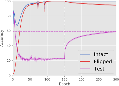
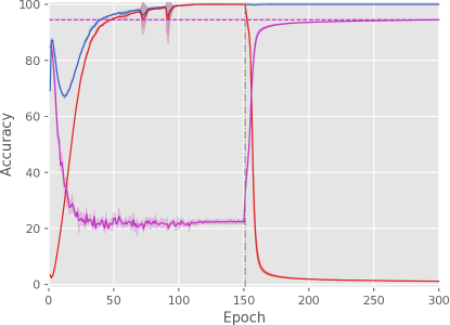
— Wide net —

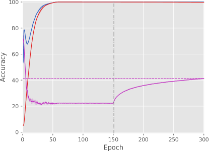
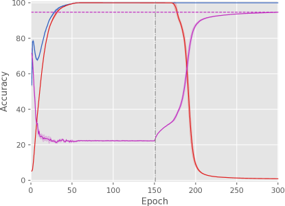
— Deep net —

Figure 1: StopGrad vs. SIGUA on noisy MNIST.

Concerning why gradient ascent is necessary or why StopGrad is inadequate, we answer it with empirical evidence. We take the MNIST benchmark dataset and add 80% symmetric label noise: for each $x_{i}$, $\mathrm{Pr}(\tilde{y}_{i}=y_{i})=0.2$ and for all $y\neq y_{i}$, $\mathrm{Pr}(\tilde{y}_{i}=y)=0.8/9$. Two neural networks are considered in this experiment:

• a wide network with an architecture 784-[Lin(10k)-BN-ReLU]-[Lin(100)-BN-ReLU]-Lin(10) which has 8,871k parameters coming from 5 trainable layers;

• a deep network with an architecture 784-[Lin(500)-BN-ReLU]*5-Lin(10) which has 1,405k parameters coming from 11 trainable layers.

Note that MNIST contains 60k training data, where 12k is intact and 48k is flipped, and thus the two neural networks are clearly over-parameterized. The base learning method $\mathfrak{B}$ is standard training that treats ${\mathcal{S}_{\mathrm{b}}}$ as drawn from $p(x,y)$ where ${n_{\mathrm{b}}}$ is 1024. The optimizer $\mathfrak{O}$ is the popular momentum SGD, where the learning rate and momentum are fixed to 0.01 and 0.9—there is no learning rate decay, otherwise StopGrad may be inadequate due to learning rate decay.

Since this experiment is for illustrating our motivation, we design ${\mathfrak{C}_{\textrm{good}}}$ and ${\mathfrak{C}_{\textrm{bad}}}$ using the true labels. The number of epochs is 300 and the shift is between 150 and 151: before the shift, we let ${\mathfrak{C}_{\textrm{good}}}(x_{i},\tilde{y}_{i})=1$, and then StopGrad and SIGUA would fit all training data; after the shift, we let

$${\mathfrak{C}_{\textrm{good}}}(x_{i},\tilde{y}_{i})=\mathbb{I}(\tilde{y}_{i}=y_{i}),\quad{\mathfrak{C}_{\textrm{bad}}}(x_{i},\tilde{y}_{i})=\mathbb{I}(\tilde{y}_{i}\neq y_{i}),$$

where $\mathbb{I}$ denotes the indicator function and it tests a conditional expression, and then they would fit only intact data. We let $\gamma=0$ for StopGrad and $\gamma=0.001$ for SIGUA, and as a result StopGrad would ignore flipped data but SIGUA would counter-fit flipped data during epochs 151–300. We repeat this random label flipping and training 5 times.

The experimental results are shown in Figure 1, where the means with standard deviations of the accuracy curves are plotted. In Figure 1, blue means training accuracy on intact data, red means that on flipped data, and purple means test accuracy on label-noise-free test data. We can see that

• the wide and deep networks can both memorize all data, while perfect memorization occurred around epoch 120 for the wide one and epoch 60 for the deep one, namely the deep memorized faster than the wide;

• in fact the wide not only memorized slower but also forgot faster, implying that its model capacity is lower than the deep, even though it has 5 times more parameters;

• at the end of training, StopGrad made the wide and deep networks forget 5% and 0% flipped data, while their test accuracy was improved from 23% to 59% and 41%;

• SIGUA made both of them forget 99% flipped data and their test accuracy was improved from 23% to 95%.

Note that MNIST contains 10 classes, so that the accuracy on flipped data lower than 10% means that perfect memorization has already been erased. Indeed, SIGUA made the accuracy on flipped data lower than 1%, which means that the model memorized a fact that the labels of those flipped data are flipped. In other words, SIGUA achieved learning with complimentary labels on those flipped data implicitly (Ishida et al., 2017; Yu et al., 2018; Ishida et al., 2019; Feng et al., 2020; Chou et al., 2020).

Lastly, the necessity of the underweight parameter $\gamma$ is for the stability of optimization. Without underweight for gradient ascent, training may be completely destroyed, if $\mathfrak{O}$ is sophisticated and uses adaptive learning rates for different parameters such as Adam (Kingma & Ba, 2015).

3 Two Realizations of SIGUA

In this section, we explain what $\mathfrak{B}$ can be used in SIGUA. We employ SIGUA to robustify self-teaching that belongs to the sample-selection approach and backward correction that belongs to the loss-correction approach. Self-teaching and backward correction are two representative and more importantly orthogonal methods in learning with noisy labels, which spotlights the great versatility of SIGUA.

SIGUA robustifies self-teaching.

The sample-selection approach regards small-loss data as “correct”, and it trains the model $f_{\theta}$ only on selected small-loss data (Jiang et al., 2018; Han et al., 2018b; Yu et al., 2019). Self-teaching, or equivalently self-paced MentorNet (Jiang et al., 2018), is the most primitive method in this direction. It maintains a single model, selects small-loss data as useful knowledge, and teaches this knowledge to itself.

In order to select small-loss data, a parameter of the label corruption process is needed—the noise level $\epsilon$ measuring how many labels are corrupted. Note that $\epsilon$ is a scalar and can be easily estimated in practice (e.g., Liu & Tao, 2016; Patrini et al., 2017). Then, the rate of data to be selected is

$$\rho(t)=1-\epsilon\cdot\min(t/T_{k},1),$$ (4)

where $t$ is the current epoch number, and $T_{k}$ is a hyperparameter denoting the number of epochs for warm-up. This means we gradually select more and more data in the first $T_{k}$ epochs, and then we select a fixed amount of data from epoch $T_{k}$, as the losses are unreliable after $f_{\theta}$ is randomly initialized and they become more and more reliable during training (Han et al., 2018b). Subsequently, let us denote by $\ell_{i}=\ell(f_{\theta}(x_{i}),\tilde{y}_{i})$ for $(x_{i},\tilde{y}_{i})\in{\mathcal{S}_{\mathrm{b}}}$ and define

$$\textstyle{\mathfrak{C}_{\textrm{good}}}(x_{i},\tilde{y}_{i})=\mathbb{I}\left(\sum_{j=1}^{n_{\mathrm{b}}}\mathbb{I}(\ell_{i}>\ell_{j})\leq{n_{\mathrm{b}}}\rho(t)\right),$$ (5)

where $\mathbb{I}(\ell_{i}>\ell_{j})$ tests if the loss on $(x_{i},\tilde{y}_{i})$ is greater than the loss on $(x_{j},\tilde{y}_{j})$, and then $\sum_{j=1}^{n_{\mathrm{b}}}\mathbb{I}(\ell_{i}>\ell_{j})$ counts how many data in ${\mathcal{S}_{\mathrm{b}}}$ have smaller losses than $\ell_{i}$. Eq. (5) is true if the count is smaller than or equal to ${n_{\mathrm{b}}}\rho(t)$, i.e., $(x_{i},\tilde{y}_{i})$ is a small-loss data in ${\mathcal{S}_{\mathrm{b}}}$. Self-teaching can be realized by plugging Eq. (5) and ${\mathfrak{C}_{\textrm{bad}}}(x_{i},\tilde{y}_{i})=0$ into Eq. (3).

Eq. (4) claims loss values can be enough informative after $T_{k}$ epochs, at which time many mislabeled data have been memorized many times. Moreover, small-loss data are just likely to be correct but not certainly, so that incorrect sample selection will mislead the model training which will in turn mislead the selection next time. As a consequence, we should employ SIGUA to robustify self-teaching. Let $\delta(t)$ be the rate of data to be forgotten, then ${\mathfrak{C}_{\textrm{bad}}}(x_{i},\tilde{y}_{i})$ can be defined similarly as

$${\mathfrak{C}_{\textrm{bad}}}(x_{i},\tilde{y}_{i})=\neg{\mathfrak{C}_{\textrm{good}}}(x_{i},\tilde{y}_{i})\land$$

$$\textstyle\qquad\mathbb{I}\left(\sum_{j=1}^{n_{\mathrm{b}}}\mathbb{I}(\ell_{i}>\ell_{j})\leq{n_{\mathrm{b}}}\rho(t)+{n_{\mathrm{b}}}\delta(t)\right),$$ (6)

where $\neg{\mathfrak{C}_{\textrm{good}}}(x_{i},\tilde{y}_{i})$ is necessary for Eq. (3) but not Algorithm 1. We refer to this self-teaching enhanced by Eq. (6) as SIGUA${{}_{\textrm{SL}}}$ where SL stands for small loss.

It seems counter-intuitive to select middle-loss data rather than large-loss data as our bad data. In fact, large-loss data are not memorized very well—no hope to confuse ${\mathfrak{C}_{\textrm{good}}}$ in Eq. (5), and then no need to be selected by ${\mathfrak{C}_{\textrm{bad}}}$ in Eq. (6). On the other hand, similarly to large-loss data, middle-loss data might be mislabeled with high probability, while they are memorized relatively well. To this end, we would like the model to slightly forget these middle-loss data, and let ${\mathfrak{C}_{\textrm{good}}}$ be less confused by them. This motivates the design of the bad-data condition ${\mathfrak{C}_{\textrm{bad}}}$ in Eq. (6).

SIGUA robustifies backward correction.

On the other hand, the loss-correction approach creates a corrected loss from $\ell$ and then trains the model $f_{\theta}$ based on the corrected loss (Patrini et al., 2017). Backward correction, for binary classification (Natarajan et al., 2013) or multi-class classification (Patrini et al., 2017), is the most primitive method in this direction. It builds ${\ell^{\leftarrow}}:\mathbb{R}^{k}\times\mathcal{Y}\to\mathbb{R}$ to reverse the label corruption process, and minimizes

$$\textstyle{\widehat{R}^{\leftarrow}}(f)=\frac{1}{n}\sum_{i=1}^{n}{\ell^{\leftarrow}}(f(x_{i}),\tilde{y}_{i}),$$ (7)

which is the corrected empirical risk.

In order to reverse the label corruption process, a model of it is needed. Note that $p(\tilde{y}\mid x)=\sum_{y}p(\tilde{y}\mid x,y)p(y\mid x)$. A model for $p(\tilde{y}\mid x,y)$ is called instance-dependent noise (cf. Menon et al., 2018; Cheng et al., 2020; Berthon et al., 2020), which is unfortunately unidentifiable without some extra assumption/information. Thus, a common practice is to assume that $p(\tilde{y}\mid x,y)=p(\tilde{y}\mid y)$, i.e., the corruption is instance-independent and class-conditional. This model is called class-conditional noise (CCN). Let $T\in\mathbb{R}_{+}^{k\times k}$ be a transition matrix such that $[T]_{i,j}=p(\tilde{y}=j\mid y=i)$. This $T$ is much more difficult to estimate than $\epsilon$, which is a hot topic in learning with noisy labels and there are still many methods (Liu & Tao, 2016; Patrini et al., 2017; Han et al., 2018a; Hendrycks et al., 2018; Xia et al., 2019; Yao et al., 2020; Xia et al., 2020). Using $T$, ${\ell^{\leftarrow}}$ is defined as

$${\ell^{\leftarrow}}(f(x),\tilde{y})=[T^{-1}{\boldsymbol{\ell}_{y\mid f(x)}}]_{\tilde{y}},$$ (8)

where ${\boldsymbol{\ell}_{y\mid f(x)}}=(\ell(f(x),1),\ldots,\ell(f(x),k))\in\mathbb{R}_{+}^{k}$, and it holds that (Patrini et al., 2017, Theorem 1)

$$\mathbb{E}_{\mathcal{S}}[{\widehat{R}^{\leftarrow}}(f)]=\mathbb{E}_{p(x,\tilde{y})}[{\ell^{\leftarrow}}(f(x),\tilde{y})]=R(f),$$ (9)

i.e., ${\widehat{R}^{\leftarrow}}(f)$ is an unbiased estimator of $R(f)$ or backward correction is risk-consistent.

Nonetheless, we should be careful of the above theoretical guarantee. Eq. (9) is about the asymptotic case rather than the finite-sample case. Note that $T^{-1}\in\mathbb{R}^{k\times k}$ though $T\in\mathbb{R}_{+}^{k\times k}$, and then ${\ell^{\leftarrow}}$ is no longer a non-negative loss. Since we are minimizing ${\ell^{\leftarrow}}(f_{\theta}(x_{i}),\tilde{y}_{i})$ where $(x_{i},\tilde{y}_{i})$ is from a finite sample $\mathcal{S}$ and $f_{\theta}$ is an over-parameterized model, the loss must go negative sooner or later whenever it could go negative (Kiryo et al., 2017; Ishida et al., 2019; Lu et al., 2020). If ${\ell^{\leftarrow}}(f_{\theta}(x_{i}),\tilde{y}_{i})$ is fairly negative, it signifies that $(x_{i},\tilde{y}_{i})$ has been memorized too much and it suggests that the optimizer $\mathfrak{O}$ should focus on the data whose losses are still positive. Consequently, we should employ SIGUA to robustify backward correction.

More specifically, we have two choices, as there is no specific good-data condition yet: one focuses on ${\ell^{\leftarrow}}(f(x),\tilde{y})$, and the other focuses on $T^{-1}{\boldsymbol{\ell}_{y\mid f(x)}}$ as a whole. We adopt the latter one, since requiring ${\ell^{\leftarrow}}(f(x),\tilde{y})\geq 0$ may be too strict and aggressive. Taking a closer look at the derivation of backward correction, we can see that for any $x$,

$${\boldsymbol{p}_{\tilde{y}\mid x}}^{\top}{\boldsymbol{\ell}_{\tilde{y}\mid f(x)}^{\leftarrow}}={\boldsymbol{p}_{y\mid x}}^{\top}{\boldsymbol{\ell}_{y\mid f(x)}},$$ (10)

where ${\boldsymbol{p}_{y\mid x}}=(p(y=1\mid x),\ldots,p(y=k\mid x))$, ${\boldsymbol{p}_{\tilde{y}\mid x}}$ is as ${\boldsymbol{p}_{y\mid x}}$, and ${\boldsymbol{\ell}_{\tilde{y}\mid f(x)}^{\leftarrow}}=T^{-1}{\boldsymbol{\ell}_{y\mid f(x)}}$. In Eq. (10), the right-hand side is always non-negative, and so should be the left-hand side. However, ${\boldsymbol{p}_{\tilde{y}\mid x}}$ is unknown to us, and thus we replace it with the uninformative uniform distribution. Finally, denote by $\boldsymbol{1}$ the all-one vector in $\mathbb{R}^{k}$, and then the good- and bad-data conditions can be defined as

$${\mathfrak{C}_{\textrm{good}}}(x_{i},\tilde{y}_{i}) =\mathbb{I}\left(\boldsymbol{1}^{\top}{\boldsymbol{\ell}_{\tilde{y}\mid f(x)}^{\leftarrow}}\geq 0\right),$$ (11)

$${\mathfrak{C}_{\textrm{bad}}}(x_{i},\tilde{y}_{i}) =\neg{\mathfrak{C}_{\textrm{good}}}(x_{i},\tilde{y}_{i}).$$ (12)

We refer to this backward correction enhanced by Eq. (11) and Eq. (12) as SIGUA${{}_{\textrm{BC}}}$.

4 Experiments

—— Symmetry-20% ——

—— Symmetry-50% ——

—— Pair-45% ——

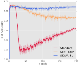
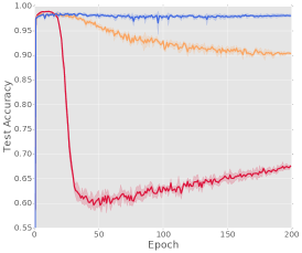
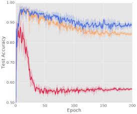
—— MNIST ——

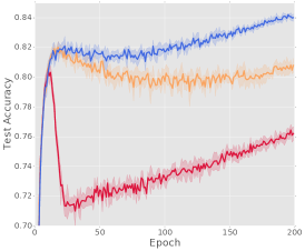
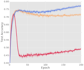
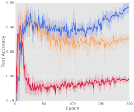
—— CIFAR-10 ——

Figure 2: Accuracy curves of training deep networks using the three learning methods in SET1.

—— Symmetry-20% ——

—— Symmetry-50% ——

—— Pair-45% ——

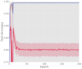
—— MNIST ——

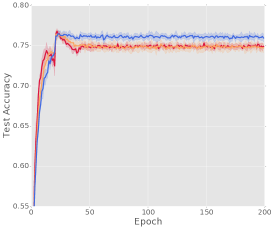
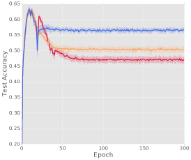
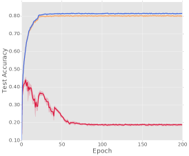
—— CIFAR-10 ——

Figure 3: Accuracy curves of training deep networks using the three learning methods in SET2.

We verify the effectiveness of SIGUA${{}_{\textrm{SL}}}$ and SIGUA${{}_{\textrm{BC}}}$ on noisy MNIST, CIFAR-10, CIFAR-100 and NEWS following Han et al. (2018b). Three noises are considered:

• under symmetry-20%, $[T]_{i,i}=0.8$ and $\forall j\neq i,[T]_{i,j}=0.2/9$, where the intact-vs-flipped margin is 0.78;

• under symmetry-50%, $[T]_{i,i}=0.5$ and $\forall j\neq i,[T]_{i,j}=0.5/9$, where the intact-vs-flipped margin is 0.44;

• under pair-45%, $[T]_{i,i}=0.55$, $[T]_{i,i\bmod 10+1}=0.45$, and other entries are 0, where the margin is 0.10.

Thus, the noises move from easy to harder until very hard. Additionally, we test SIGUA${{}_{\textrm{SL}}}$ and SIGUA${{}_{\textrm{BC}}}$ on the more challenging open-set setting (Wang et al., 2018; Lee et al., 2019) by replacing CIFAR-10 images with SVHN images while keeping the labels of those “mislabeled” data intact.

According to the learning methods being involved, the experiments can be divided into two sets. SET1 involves

• standard training with ${\mathfrak{C}_{\textrm{good}}}\equiv 1,{\mathfrak{C}_{\textrm{bad}}}\equiv 0$,

• self-teaching with ${\mathfrak{C}_{\textrm{good}}}$ as Eq. (5) and ${\mathfrak{C}_{\textrm{bad}}}\equiv 0$,

• SIGUA${{}_{\textrm{SL}}}$ with ${\mathfrak{C}_{\textrm{good}}}$ as Eq. (5) and ${\mathfrak{C}_{\textrm{bad}}}$ as Eq. (6).

The first method is $\mathfrak{B}$ in this set where the surrogate loss $\ell$ is softmax cross-entropy loss. For $\rho(t)$ in Eq. (4), $T_{k}=10$ and $\epsilon$ is given as its true value; $\delta(t)$ is a constant independent of $t$ and depends only on the dataset. SET2 involves

• backward correction (BC) with ${\mathfrak{C}_{\textrm{good}}}\equiv 1,{\mathfrak{C}_{\textrm{bad}}}\equiv 0$,

• non-negative backward correction (nnBC) with ${\mathfrak{C}_{\textrm{good}}}$ as Eq. (11) and ${\mathfrak{C}_{\textrm{bad}}}\equiv 0$,

• SIGUA${{}_{\textrm{BC}}}$ with ${\mathfrak{C}_{\textrm{good}}}$ as Eq. (11) and ${\mathfrak{C}_{\textrm{bad}}}$ as Eq. (12).

The first method is $\mathfrak{B}$ in this set where $\ell$ in Eq. (8) is again softmax cross-entropy loss. $T$ is given as its true value for constructing ${\ell^{\leftarrow}}$ in Eq. (8). Note that our experiments are proof-of-concept, and the baselines are just chosen for this purpose. In principle, SIGUA can robustify other methods (e.g., Reed et al., 2015; Goldberger & Ben-Reuven, 2017; Hendrycks et al., 2019) provided that we could distinguish desired and undesired memorization conceptually.

The six learning methods are implemented using PyTorch. In SET1, $\mathfrak{O}$ is Adam (Kingma & Ba, 2015) in its default, and the number of epochs is 200 with batch size ${n_{\mathrm{b}}}$ as 128; the learning rate is linearly decayed to 0 from epoch 80 to 200. We set $\gamma=0.01$ for all cases, except that $\gamma=0.001$ for pair-45% of MNIST. SET2 is a bit complicated:

• for MNIST, $\mathfrak{O}$ is Adam with betas as (0.9, 0.1), and lr is divided by 10 every 10 epochs;

• for CIFAR-10, $\mathfrak{O}$ is SGD with momentum as 0.9, and lr is divided by 10 every 20 epochs;

• other hyperparameters have the same values as in SET1.

We simply set $\gamma=1.0$ for all cases. Neural network architectures for benchmark datasets are given in Appendix A. Data augmentation is excluded from consideration (cf. Ma et al., 2018; Zhang & Sabuncu, 2018), as our experiments are proof-of-concept. Due to the limited space, the experiments on CIFAR-100 and NEWS are completely deferred to Appendix B. All the experiments are repeated five times and the mean accuracy with standard deviation is recorded for each method in SET1 or SET2.

SET1 results.

Figure 2 shows the accuracy curves of the three methods in SET1 (MNIST in the top and CIFAR-10 in the bottom). We can clearly see in Figure 2 that models learned patterns first, and hence a robust learning method should be able to stop (or alleviate) the accuracy decrease. On this point, SIGUA${{}_{\textrm{SL}}}$ stopped the decrease in Standard and Self-Teach under two symmetry cases, and alleviated the decrease under pair-45%, on MNIST. SIGUA${{}_{\textrm{SL}}}$ did a particularly good job on CIFAR-10, where it successfully made the accuracy continue to increase without a remarkable decrease, which indicates that SIGUA${{}_{\textrm{SL}}}$ is superior to early stopping. Table 1 shows the average accuracy under the open-set noise and we can see SIGUA${{}_{\textrm{SL}}}$ outperformed Self-Teach significantly. In summary, SIGUA consistently improved Self-Teach under the easy, harder, and very hard noises (note that the scales of y-axis are different), and the improvements were always significant.

Table 1: Average test accuracy (in %) over the last ten epochs on CIFAR-10 under 40% open-set noise from SVHN.

Standard	Self	SIGUA${{}_{\textrm{SL}}}$	BC	nnBC	SIGUA${{}_{\textrm{BC}}}$
56.44	79.72	81.31	52.03	73.39	74.33

SET2 results.

Figure 3 shows the accuracy curves of the three methods in SET2. Surprisingly, models trained with BC still learned patterns first, even though $\ell$ was corrected into ${\ell^{\leftarrow}}$. This implies there should be some other cause of overfitting (since Eq. (10) holds for any $x$), and indeed the cause is negative ${\ell^{\leftarrow}}$ on certain $(x_{i},\tilde{y}_{i})$. In Figure 3, nnBC was sometimes good enough but sometimes not enough to stop or alleviate the accuracy decrease, since nnBC tries to ignore rather than fix any negative loss. SIGUA${{}_{\textrm{BC}}}$ stopped the decrease in 5 cases and alleviated it in 1 case by fixing negative losses. In Table 1, we can also see that SIGUA${{}_{\textrm{BC}}}$ outperformed BC and nnBC significantly. In order to sum up, SIGUA consistently improved BC/nnBC under different noises, and the improvements were often significant.

Comparing results from SET1 and SET2.

Note that $\epsilon$ or $T$ is given to SET1 or SET2 methods, and thus there is no error in estimating the label corruption process. We can roughly see on MNIST, the performance of SIGUA${{}_{\textrm{SL}}}$ and SIGUA${{}_{\textrm{BC}}}$ were very close under two symmetry cases, but SIGUA${{}_{\textrm{BC}}}$ was superior under pair-45%; on CIFAR-10, the performance of SIGUA${{}_{\textrm{BC}}}$ was inferior to SIGUA${{}_{\textrm{SL}}}$ under symmetry cases and again superior under pair-45%.

This is because the small-loss criterion is more reliable under symmetry noises than pair noises, where the reliability is determined by the intact-vs-flipped margin more than by the noise level $\epsilon$. On the other hand, Eq. (8) for constructing ${\ell^{\leftarrow}}$ is equally reliable under different noises as long as the noise belongs to CCN. This explains why SET2 methods were remarkably outperformed by SET1 methods under open-set noise—this noise does not even belong to the label noise, let alone CCN. Actually, sample selection is a bit more general than loss correction and label correction, in a sense that it serves as corrections for not only flipping $y$ in label noise but also replacing $x$ in open-set noise.

Last but not least, comparing SET1 and SET2, we can find that desired memorization is not a concept definitely associated with intact data, and then neither is undesired memorization definitely associated with flipped data.

Table 2: Average test accuracy w. std dev (in %) over the last ten epochs of supervised learning, SIGUA${{}_{\textrm{SL}}}$ and SIGUA${{}_{\textrm{BC}}}$.

MNIST	Symmetry-20%	Symmetry-50%	Pair-45%
Supervised	99.61 (0.02)	99.61 (0.02)	99.61 (0.02)
SIGUA${{}_{\textrm{SL}}}$	98.91 (0.19)	98.10 (0.30)	89.37 (0.82)
SIGUA${{}_{\textrm{BC}}}$	99.42 (0.10)	97.73 (0.05)	99.47 (0.02)

Table 3: Average test accuracy w. std dev (in %) over the last ten epochs of SIGUA${{}_{\textrm{BC}}}$ and robust-loss-based learning methods.

MNIST	Symmetry-20%	Symmetry-50%	Pair-45%
SIGUA${{}_{\textrm{BC}}}$	99.42 (0.10)	97.73 (0.05)	99.47 (0.02)
Huber	93.61 (0.25)	65.38 (0.33)	56.48 (0.67)
Log-sum	94.35 (0.12)	67.46 (0.40)	57.38 (0.33)

Comparison with supervised learning.

Next, we investigate the performance gap between SIGUA and the oracle supervised learning with clean labels. In supervised learning, we train the same model using the same optimizer but on label-noise-free training data, and thus its performance upper bounds the performance of any learning method, no matter existing or to be proposed in the future, for learning with noisy labels. The results are shown in Table 3, where SIGUA approximately approached the performance of supervised learning and achieved a rather small performance gap. It is not surprised, as MNIST is an easy dataset, CCN is a relatively easy noise to correct, and $T$ is given. In this research area, instance-dependent noise is worth us to pay more attention; within CCN the bottleneck/focus is how to estimate $T$ more and more accurately (Xia et al., 2019).

Comparison with robust losses.

In the end, ${\ell^{\leftarrow}}$ is compared with Huber loss and log-sum loss for robust regression (Candes et al., 2008). To make use of them, let $\boldsymbol{y}$ and $\boldsymbol{\tilde{y}}$ be the one-hot vectors of $y$ and $\tilde{y}$, and $\ell(f(x),\boldsymbol{\tilde{y}})$ be the sum of Huber/log-sum losses from $k$ dimensions ($f$ itself is vector-valued). The assumed noise model is additive by these losses: $\boldsymbol{y}$ and $\boldsymbol{\tilde{y}}$ are continuous and their difference $\boldsymbol{\epsilon}$ is sampled from $(1-\epsilon)\mathcal{N}(\boldsymbol{0},\sigma I)+\epsilon\mathcal{N}(\boldsymbol{0},\sigma^{\prime}I)$ where $\mathcal{N}$ denotes the multivariate normal distribution, $\boldsymbol{0}$ denotes the all-zero vector in $\mathbb{R}^{k}$, and $\sigma\ll\sigma^{\prime}$ for covariance matrices. The results are shown in Table 3, where two robust losses notably failed under symmetry-50% and pair-45%. It is as expected, since they are specially designed to be robust to outliers or similar additive noises, whereas ${\ell^{\leftarrow}}$ is specially designed to be robust to flipping noises.

5 Conclusions

We presented in this paper a versatile approach to learning with noisy labels called SIGUA. By carefully distinguishing desired and undesired memorization, SIGUA was successful in robustifying two typical base learning methods: self-teaching from sample selection, and backward correction from loss correction. We demonstrated through experiments that two enhanced methods can result in significant improvements. In general, SIGUA can be applied to other methods or even other problem settings like learning from similarity-unlabeled data (e.g., Bao et al., 2018) and pairwise comparison data (e.g., Xu et al., 2019).

SIGUA exhibits pulling optimization back for generalization in learning with noisy labels. There should be a trade-off between them implemented as an equilibrium between gradient descent and ascent, and then the model will travel between (uncountably infinite) reasonably good solutions, where the goodness is in the sense of optimization instead of generalization. See Ishida et al. (2020) for a dedicated study of this phenomenon in supervised learning.

Appendix A Neural Network Architectures for Benchmark Datasets

Table 4: CNN on MNIST and CIFAR-10/100.

Input	28$\times$28 Gray Image
	32$\times$32 Color Image
Block 1	Conv(3$\times$3, 128)-BN-LReLU
	Conv(3$\times$3, 128)-BN-LReLU
	Conv(3$\times$3, 128)-BN-LReLU
	MaxPool(2$\times$2, stride = 2)
	Dropout(p = 0.25)
Block 2	Conv(3$\times$3, 256)-BN-LReLU
	Conv(3$\times$3, 256)-BN-LReLU
	Conv(3$\times$3, 256)-BN-LReLU
	MaxPool(2$\times$2, stride = 2)
	Dropout(p = 0.25)
Block 3	Conv(3$\times$3, 512)-BN-LReLU
	Conv(3$\times$3, 256)-BN-LReLU
	Conv(3$\times$3, 128)-BN-LReLU
	GlobalAvgPool(128)
Score	Linear(128, 10 or 100)

Table 5: CNN for open-set noise.

Input	32$\times$32 Color Image
Block 1	Conv(3$\times$3, 64)-BN-LReLU
	Conv(3$\times$3, 64)-BN-LReLU
	MaxPool(2$\times$2)
Block 2	Conv(3$\times$3, 128)-BN-LReLU
	Conv(3$\times$3, 128)-BN-LReLU
	MaxPool(2$\times$2)
Block 3	Conv(3$\times$3, 196)-BN-LReLU
	Conv(3$\times$3, 196)-BN-LReLU
	MaxPool(2$\times$2)
Score	Linear(256, 10)

Table 6: 1D CNN on NEWS.

Input	Sequence of Tokens
Embed	300D GloVe
Block 1	Conv(3, 100)-ReLU
	GlobalMaxPool(100)
Score	Linear(100, 7)

Table 7: MLP on NEWS.

Input	Sequence of Tokens
Embed	300D GloVe
Block 1	Linear(300, 300)-Softsign
	Linear(300, 300)-Softsign
Score	Linear(300, 2)

Table 7 describes the 9-layer CNN (Laine & Aila, 2017; Miyato et al., 2019) used on MNIST and CIFAR-10/100. In fact, it has 9 convolutional layers but 19 trainable layers. Table 7 describes the CNN used on CIFAR-10 under open-set noise. It has 6 convolutional layers but 13 trainable layers. Furthermore, the 1D CNN on NEWS for SET1 methods and MLP on NEWS for SET2 methods are given in Tables 7 and 7 respectively. Here, BN stands for batch normalization layers (Ioffe & Szegedy, 2015); LReLU stands for Leaky ReLU (Xu et al., 2015), a special case of Parametric ReLU (He et al., 2015); GloVe stands for global vectors for word representation (Pennington et al., 2014); Softsign is an activation function which looks very similar to Tanh (Glorot & Bengio, 2010).

Note that the 9-layer CNN is a standard and common practice in weakly supervised learning, including but not limited to semi-supervised learning (e.g., Laine & Aila, 2017; Miyato et al., 2019) and noisy-label learning (e.g., Han et al., 2018b). Actually, this CNN was not born in those areas—it came from Salimans et al. (2016) where it served as the discriminator of GANs on CIFAR-10. We decided to use this CNN, because then the experimental results are directly comparable with previous papers in the same area, and it would be crystal clear where the proposed methods stand in the area.

That being said, SIGUA can definitely achieve better performance if given better models. In order to demonstrate this, let us take ResNet-18 (He et al., 2016), the smallest ResNet in torch vision model zoo for example. The experimental results are shown in Table 8. For each noise, we selected the better one among SIGUA${{}_{\textrm{SL}}}$ and SIGUA${{}_{\textrm{BC}}}$, and replaced the model with ResNet-18. We can see from Table 8 that the improvements were very great by training bigger ResNet-18.

Table 8: Average test accuracy (in %) over the last ten epochs on CIFAR-10.

	SIGUA${{}_{\textrm{SL}}}$ under	SIGUA${{}_{\textrm{SL}}}$ under	SIGUA${{}_{\textrm{BC}}}$
	symmetry-20%	symmetry-50%	under pair-45%
9-layer CNN	84.05	77.12	81.82
ResNet-18	89.41	81.96	89.56
Absolute Acc Increase	5.36	4.84	7.74
Relative Err Reduction	33.61	21.15	42.57

Appendix B More Experiments

—— Symmetry-20% ——

—— Symmetry-50% ——

—— Pair-45% ——

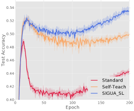
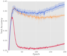
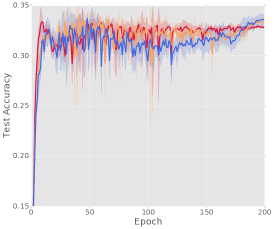
—— CIFAR-100 ——

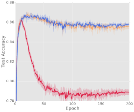
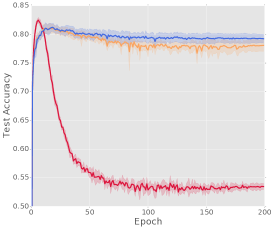
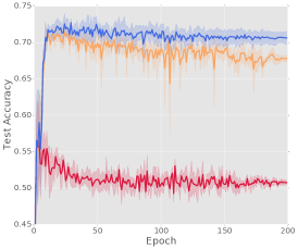
—— NEWS ——

Figure 4: Accuracy curves of training deep networks using the three learning methods in SET1.

—— Symmetry-20% ——

—— Symmetry-50% ——

—— Pair-45% ——

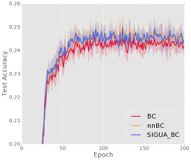
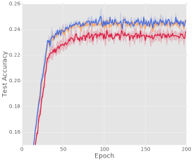
—— CIFAR-100 ——

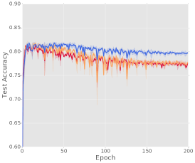
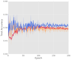
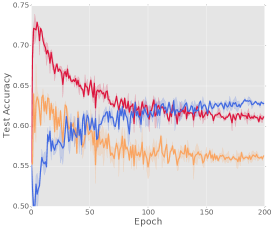
—— NEWS ——

Figure 5: Accuracy curves of training deep networks using the three learning methods in SET2.

Due to the limited space, the experiments on CIFAR-100 and NEWS are moved here. The setup of CIFAR-100 is similar to CIFAR-10, but the momentum is 0.5 and lr is divided by 10 every 30 epochs for SET2 methods. The setup of NEWS is similar to other three datasets, except $\mathfrak{O}$ is AdaGrad (Duchi et al., 2011) that automatically decays lr every mini-batch.

Figure 5 shows the accuracy curves of the three methods in SET1 (CIFAR-100 in the top and NEWS in the bottom). The trend in Figure 5 is similar to the trend in Figure 2 that SIGUA${{}_{\textrm{SL}}}$ either stopped or alleviated the decrease in Standard and Self-Teach. Especially on CIFAR-100, after a remarkable decrease in the first half, the accuracy in the second half started to increase once more, and it eventually surpassed the best accuracy that can be obtained by early stopping. If we plot the test error rather than the test accuracy, this phenomenon is exactly an epoch-wise double descent (Nakkiran et al., 2020). Figure 5 shows the accuracy curves of the three methods in SET2 where SIGUA${{}_{\textrm{BC}}}$ still stopped or alleviated the decrease in BC and/or nnBC. The reason why BC suffered more under pair-45% may be explained by the maximum and minimum elements of $T^{-1}$: when $k=10$, they are 2.101 and -1.719 under pair-45% but 2.125 and -0.125 under symmetry-50%. It is interesting on CIFAR-10, nnBC and SIGUA${{}_{\textrm{BC}}}$ under pair-45% outperformed themselves under symmetry-20%, which provides an evidence that the issue of negative losses can be fixed at least empirically.

References

- Arpit et al. (2017) Arpit, D., Jastrzebski, S., Ballas, N., Krueger, D., Bengio, E., Kanwal, M., Maharaj, T., Fischer, A., Courville, A., and Bengio, Y. A closer look at memorization in deep networks. In ICML, 2017.
- Bao et al. (2018) Bao, H., Niu, G., and Sugiyama, M. Classification from pairwise similarity and unlabeled data. In ICML, 2018.
- Berthon et al. (2020) Berthon, A., Han, B., Niu, G., Liu, T., and Sugiyama, M. Confidence scores make instance-dependent label-noise learning possible. arXiv:2001.03772, 2020.
- Candes et al. (2008) Candes, E., Wakin, M., and Boyd, S. Enhancing sparsity by reweighted l1 minimization. Journal of Fourier analysis and applications, 14(5-6):877–905, 2008.
- Cheng et al. (2020) Cheng, J., Liu, T., Ramamohanarao, K., and Tao, D. Learning with bounded instance- and label-dependent label noise. In ICML, 2020.
- Chou et al. (2020) Chou, Y.-T., Niu, G., Lin, H.-T., and Sugiyama, M. Unbiased risk estimators can mislead: A case study of learning with complementary labels. In ICML, 2020.
- du Plessis et al. (2014) du Plessis, M. C., Niu, G., and Sugiyama, M. Analysis of learning from positive and unlabeled data. In NeurIPS, 2014.
- Duchi et al. (2011) Duchi, J., Hazan, E., and Singer, Y. Adaptive subgradient methods for online learning and stochastic optimization. Journal of Machine Learning Research, 12:2121–2159, 2011.
- Feng et al. (2020) Feng, L., Kaneko, T., Han, B., Niu, G., An, B., and Sugiyama, M. Learning with multiple complementary labels. In ICML, 2020.
- Glorot & Bengio (2010) Glorot, X. and Bengio, Y. Understanding the difficulty of training deep feedforward neural networks. In AISTATS, 2010.
- Goldberger & Ben-Reuven (2017) Goldberger, J. and Ben-Reuven, E. Training deep neural-networks using a noise adaptation layer. In ICLR, 2017.
- Goodfellow et al. (2016) Goodfellow, I., Bengio, Y., and Courville, A. Deep learning. MIT Press, 2016.
- Han et al. (2018a) Han, B., Yao, J., Niu, G., Zhou, M., Tsang, I., Zhang, Y., and Sugiyama, M. Masking: A new perspective of noisy supervision. In NeurIPS, 2018a.
- Han et al. (2018b) Han, B., Yao, Q., Yu, X., Niu, G., Xu, M., Hu, W., Tsang, I., and Sugiyama, M. Co-teaching: Robust training of deep neural networks with extremely noisy labels. In NeurIPS, 2018b.
- He et al. (2015) He, K., Zhang, X., Ren, S., and Sun, J. Delving deep into rectifiers: Surpassing human-level performance on imagenet classification. In CVPR, 2015.
- He et al. (2016) He, K., Zhang, X., Ren, S., and Sun, J. Deep residual learning for image recognition. In CVPR, 2016.
- Hendrycks et al. (2018) Hendrycks, D., Mazeika, M., Wilson, D., and Gimpel, K. Using trusted data to train deep networks on labels corrupted by severe noise. In NeurIPS, 2018.
- Hendrycks et al. (2019) Hendrycks, D., Lee, K., and Mazeika, M. Using pre-training can improve model robustness and uncertainty. In ICML, 2019.
- Ioffe & Szegedy (2015) Ioffe, S. and Szegedy, C. Batch normalization: Accelerating deep network training by reducing internal covariate shift. In ICML, 2015.
- Ishida et al. (2017) Ishida, T., Niu, G., Hu, W., and Sugiyama, M. Learning from complementary labels. In NeurIPS, 2017.
- Ishida et al. (2019) Ishida, T., Niu, G., Menon, A. K., and Sugiyama, M. Complementary-label learning for arbitrary losses and models. In ICML, 2019.
- Ishida et al. (2020) Ishida, T., Yamane, I., Sakai, T., Niu, G., and Sugiyama, M. Do we need zero training loss after achieving zero training error? In ICML, 2020.
- Jiang et al. (2018) Jiang, L., Zhou, Z., Leung, T., Li, L., and Fei-Fei, L. Mentornet: Learning data-driven curriculum for very deep neural networks on corrupted labels. In ICML, 2018.
- Kingma & Ba (2015) Kingma, D. and Ba, J. Adam: A method for stochastic optimization. In ICLR, 2015.
- Kiryo et al. (2017) Kiryo, R., Niu, G., du Plessis, M. C., and Sugiyama, M. Positive-unlabeled learning with non-negative risk estimator. In NeurIPS, 2017.
- Krogh & Hertz (1991) Krogh, A. and Hertz, J. A. A simple weight decay can improve generalization. In NeurIPS, 1991.
- Laine & Aila (2017) Laine, S. and Aila, T. Temporal ensembling for semi-supervised learning. In ICLR, 2017.
- Lee et al. (2019) Lee, K., Yun, S., Lee, K., Lee, H., Li, B., and Shin, J. Robust inference via generative classifiers for handling noisy labels. In ICML, 2019.
- Liu & Tao (2016) Liu, T. and Tao, D. Classification with noisy labels by importance reweighting. IEEE Transactions on Pattern Analysis and Machine Intelligence, 38(3):447–461, 2016.
- Lu et al. (2020) Lu, N., Zhang, T., Niu, G., and Sugiyama, M. Mitigating overfitting in supervised classification from two unlabeled datasets: A consistent risk correction approach. In AISTATS, 2020.
- Ma et al. (2018) Ma, X., Wang, Y., Houle, M., Zhou, S., Erfani, S., Xia, S., Wijewickrema, S., and Bailey, J. Dimensionality-driven learning with noisy labels. In ICML, 2018.
- Menon et al. (2018) Menon, A. K., van Rooyen, B., and Natarajan, N. Learning from binary labels with instance-dependent corruption. Machine Learning, 107:1561–1595, 2018.
- Miyato et al. (2019) Miyato, T., Maeda, S., Ishii, S., and Koyama, M. Virtual adversarial training: a regularization method for supervised and semi-supervised learning. IEEE Transactions on Pattern Analysis and Machine Intelligence, 41(8):1979–1993, 2019.
- Morgan & Bourlard (1990) Morgan, N. and Bourlard, H. Generalization and parameter estimation in feedforward nets: Some experiments. In NeurIPS, 1990.
- Nakkiran et al. (2020) Nakkiran, P., Kaplun, G., Bansal, Y., Yang, T., Barak, B., and Sutskever, I. Deep double descent: Where bigger models and more data hurt. In ICLR, 2020.
- Natarajan et al. (2013) Natarajan, N., Dhillon, I., Ravikumar, P., and Tewari, A. Learning with noisy labels. In NeurIPS, 2013.
- Niu et al. (2016) Niu, G., du Plessis, M. C., Sakai, T., Ma, Y., and Sugiyama, M. Theoretical comparisons of positive-unlabeled learning against positive-negative learning. In NeurIPS, 2016.
- Patrini et al. (2017) Patrini, G., Rozza, A., Menon, A., Nock, R., and Qu, L. Making deep neural networks robust to label noise: a loss correction approach. In CVPR, 2017.
- Pennington et al. (2014) Pennington, J., Socher, R., and Manning, C. D. GloVe: Global vectors for word representation. In EMNLP, 2014.
- Reed et al. (2015) Reed, S., Lee, H., Anguelov, D., Szegedy, C., Erhan, D., and Rabinovich, A. Training deep neural networks on noisy labels with bootstrapping. In ICLR, 2015.
- Robbins & Monro (1951) Robbins, H. and Monro, S. A stochastic approximation method. The Annals of Mathematical Statistics, 22(3):400–407, 1951.
- Salimans et al. (2016) Salimans, T., Goodfellow, I., Zaremba, W., Cheung, V., Radford, A., Chen, X., and Chen, X. Improved techniques for training gans. In NeurIPS, 2016.
- Srivastava et al. (2014) Srivastava, N., Hinton, G., Krizhevsky, A., Sutskever, I., and Salakhutdinov, R. Dropout: a simple way to prevent neural networks from overfitting. Journal of Machine Learning Research, 15(56):1929–1958, 2014.
- Suzuki (2019) Suzuki, T. Adaptivity of deep ReLU network for learning in Besov and mixed smooth Besov spaces: optimal rate and curse of dimensionality. In ICLR, 2019.
- Tokui et al. (2015) Tokui, S., Oono, K., Hido, S., and Clayton, J. Chainer: a next-generation open source framework for deep learning. In NeurIPS Workshop on Machine Learning Systems, 2015.
- Vapnik (1998) Vapnik, V. N. Statistical Learning Theory. John Wiley & Sons, 1998.
- Wang et al. (2018) Wang, Y., Liu, W., Ma, X., Bailey, J., Zha, H., Song, L., and Xia, S. Iterative learning with open-set noisy labels. In CVPR, 2018.
- Wang et al. (2019) Wang, Y., Ma, X., Chen, Z., Luo, Y., Yi, J., and Bailey, J. Symmetric cross entropy for robust learning with noisy labels. In ICCV, 2019.
- Welinder et al. (2010) Welinder, P., Branson, S., Perona, P., and Belongie, S. The multidimensional wisdom of crowds. In NeurIPS, 2010.
- Xia et al. (2019) Xia, X., Liu, T., Wang, N., Han, B., Gong, C., Niu, G., and Sugiyama, M. Are anchor points really indispensable in label-noise learning? In NeurIPS, 2019.
- Xia et al. (2020) Xia, X., Liu, T., Han, B., Wang, N., Gong, M., Liu, H., Niu, G., Tao, D., and Sugiyama, M. Parts-dependent label noise: Towards instance-dependent label noise. arXiv:2006.07836, 2020.
- Xiao et al. (2015) Xiao, T., Xia, T., Yang, Y., Huang, C., and Wang, X. Learning from massive noisy labeled data for image classification. In CVPR, 2015.
- Xu et al. (2015) Xu, B., Wang, N., Chen, T., and Li, M. Empirical evaluation of rectified activations in convolutional network. In ICML Deep Learning Workshop, 2015.
- Xu et al. (2019) Xu, L., Honda, J., Niu, G., and Sugiyama, M. Uncoupled regression from pairwise comparison data. In NeurIPS, 2019.
- Yao et al. (2020) Yao, Y., Liu, T., Han, B., Gong, M., Deng, J., Niu, G., and Sugiyama, M. Dual T: Reducing estimation error for transition matrix in label-noise learning. arXiv:2006.07805, 2020.
- Yu et al. (2018) Yu, X., Liu, T., Gong, M., and Tao., D. Learning with biased complementary labels. In ECCV, 2018.
- Yu et al. (2019) Yu, X., Han, B., Yao, J., Niu, G., Tsang, I. W., and Sugiyama, M. How does disagreement help generalization against label corruption? In ICML, 2019.
- Zhang et al. (2017) Zhang, C., Bengio, S., Hardt, M., Recht, B., and Vinyals, O. Understanding deep learning requires rethinking generalization. In ICLR, 2017.
- Zhang & Sabuncu (2018) Zhang, Z. and Sabuncu, M. Generalized cross entropy loss for training deep neural networks with noisy labels. In NeurIPS, 2018.