Triangle singularity in $\tau^{-}\to\nu_{\tau}\pi^{-}f_{0}(980)$ ($a_{0}(980)$) decays

Abstract

We study the triangle mechanism for the decay $\tau^{-}\to\nu_{\tau}\pi^{-}f_{0}(980)$, with the $f_{0}(980)$ decaying into $\pi^{+}\pi^{-}$. This process is initiated by $\tau^{-}\to\nu_{\tau}K^{*0}K^{-}$ followed by the $K^{*0}$ decay into $\pi^{-}K^{+}$, then the $K^{-}K^{+}$ produce the $f_{0}(980)$ through a triangle loop containing $K^{*}K^{+}K^{-}$ which develops a singularity around $1420$ MeV in the $\pi f_{0}(980)$ invariant mass. We find a narrow peak in the $\pi^{+}\pi^{-}$ invariant mass distribution, which originates from the $f_{0}(980)$ amplitude. Similarly, we also study the triangle mechanism for the decay $\tau\to\nu\pi^{-}a_{0}(980)$, with the $a_{0}(980)$ decaying into $\pi^{0}\eta$. The final branching ratios for $\pi^{-}f_{0}(980)$ and $\pi^{-}a_{0}(980)$ are of the order of $4\times 10^{-4}$ and $7\times 10^{-5}$, respectively, which are within present measurable range. Experimental verification of these predictions will shed light on the nature of the scalar mesons and on the origin for the “$a_{1}(1420)$” peak observed in other reactions.

I Introduction

Triangle singularities were studied in detail by Landau [1] and they emerge from a process symbolized by a triangle Feynman diagram in which one particle decays into $1$ and $R$, $R$ decays later into $2+3$ and $1+2$ merge to give another state, or simply rescatter. Under certain conditions where all particles $1,2,3$ can be placed on shell, $1$ and $3$ are antiparallel and the process can occur at the classical level [2] (Coleman Norton Theorem), the process develops a singularity visible in a peak in the corresponding cross sections. While no clear such physical processes were observed for a long time, the situation reverted recently where clear cases have been observed and many reactions have been suggested to show such phenomena. A particular case is the triangle singularity studied in [3, 5, 4] where a peak seen by the COMPASS collaboration in the $\pi f_{0}(980)$ final state [6], branded originally as a new resonance, “$a_{1}(1420)$” , was naturally explained in terms of the triangle singularity stemming from the original production of $K^{*}\bar{K}$, decay of $K^{*}$ into $\pi K$ and fusion of $K\bar{K}$ to give the $f_{0}(980)$ resonance.

The interest in triangle singularities has grown recently. In addition to the interpretation of the “$a_{1}(1420)$” as a triangle singularity, the $f_{1}(1420)$, officially in the PDG tables [7] was also shown to correspond to the “$f_{1}(1285)$” decay into $K^{*}\bar{K}$, with the “$\pi a_{0}(980)$ decay width” [8] also corresponding to the “$f_{1}(1285)$” [9]. Similarly the “$f_{2}(1810)$” was also shown to come from a triangle singularity [10]. Some particular reactions have also been studied and partial contributions or peaks in the cross sections have also been associated to triangle singularities, and suggestions of new reactions to see them have been proposed [11, 12, 13, 14, 15, 16, 17, 18, 19, 20, 21, 22, 23, 24, 25, 26, 27, 28, 29].

In the present work we study the reactions $\tau^{-}\to\nu_{\tau}\pi^{-}f_{0}(980)$ and $\tau^{-}\to\nu_{\tau}\pi^{-}a_{0}(980)$. The original $\tau^{-}$ decays into a $\nu_{\tau}$ and a $d\bar{u}$ state that has $I_{3}=-1,I=1$. The further hadronization including a $\bar{q}q$ pair forms two mesons conserving isospin. Hence, both decays modes are allowed. Since $f_{0}(980)$, $a_{0}(980)$ couple mostly to $K\bar{K}$, the reaction requires the formation of this pair, in addition to the $\pi^{-}$. Hence it proceeds via $K^{*}\bar{K}$ production, followed by $K^{*}$ decay to $\pi^{-}K$ and the $K\bar{K}$ fuse to produce the $f_{0}(980)$ or the $a_{0}(980)$. Then we have a triangle mechanism that could or not produce a singularity. However we show that it develops a triangle singularity at an invariant mass $M_{\rm inv}(\pi R)(R\equiv f_{0},a_{0})\simeq 1420$ MeV. Interestingly, the triangle mechanism that produces a peak in this invariant mass distribution is the same one that produced the “$a_{1}(1420)$” peak observed in the COMPASS experiment.

The other issue present in this reaction is the $G$-parity. The $\pi^{-}f_{0}(980)$ and $\pi^{-}a_{0}(980)$ have negative and positive $G$-parity respectively. The formalism has to provide the means to filter the states of $G$-parity just after the weak decay, from the operators involved in the $Wd\bar{u}$ vertex. Fortunately a formalism has been developed recently [30] in which the $G$-parity appears explicitly in the amplitudes written at the macroscopic meson level after the hadronization to produce two mesons. By means of this formalism we can easily evaluate the loops involved in the triangle mechanism and predict quantitative mass distributions for the $\tau^{-}$ decay in these modes. This is made possible because the radial matrix elements of the quark wave functions, which are a source of large uncertainties and we do not explicitly evaluate, are implicitly taken into account by making use of the experimental value of the $\tau\to\nu_{\tau}K^{*0}K^{-}$ branching ratio, which is the first step in our loop mechanism.

By means of this approach we obtain $\frac{d^{2}\Gamma}{dM_{\text{inv}}(\pi^{-}R)dM_{\text{inv}}(\pi^{+}\pi^{-})}$ or $\frac{d^{2}\Gamma}{dM_{\text{inv}}(\pi^{-}R)dM_{\text{inv}}(\pi^{0}\eta)}$ which show the shapes of the $f_{0}(980)$ and $a_{0}(980)$ resonances in the $\pi^{+}\pi^{-}$ or $\pi^{0}\eta$ mass distributions respectively. Then we integrate over the $\pi^{+}\pi^{-}$ or $\pi^{0}\eta$ invariant masses and obtain $\frac{d^{2}\Gamma}{dM_{\text{inv}}(\pi^{-}R)}$, which shows a clear peak around $M_{\text{inv}}(\pi^{-}R)\simeq 1420$ MeV. The further integration over $M_{\text{inv}}(\pi^{-}R)$ provides us branching ratios for $\tau^{-}\to\nu_{\tau}\pi^{-}f_{0}(980)$ and $\tau^{-}\to\nu_{\tau}\pi^{-}a_{0}(980)$ production, and we obtain values of $4\times 10^{-4}$ and $7\times 10^{-5}$ for these two ratios respectively, which are well within measurable range.

The measurement of such reactions and comparison with the present results should be very useful since it conjugates several interesting issues:

i

It provides one more measurable example of a triangle singularity, which have been quite sparse up to now.

ii

It serves as a further test of the nature of the $f_{0}(980)$ and $a_{0}(980)$, since they are not directly produced from the weak decay, but come from fusion of $K\bar{K}$ in a scattering process, establishing a link with the chiral unitary approach to these resonances where they are shown not to correspond to $q\bar{q}$ state but are generated by the scattering of pseudoscalar mesons in coupled channels.

iii

The filters of the $G$-parity in the amplitudes can also provide information that can be extrapolated to $\tau^{-}\to\nu_{\tau}M_{1}M_{2}$ decays with $M_{1}M_{2}$ pairs of states that have a given $G$-parity as $\pi\rho$, $\pi\omega$, $\eta\rho$ and $\eta^{\prime}\rho$.

With the possible advent of a future $\tau^{-}$ facility, predictions like the present one and the motivation given, should provide the grounds for proposals at that machine. Yet, other existing facilities have also access to these reactions since rates of $10^{-5}$ and smaller are common in $\tau^{-}$ decays [7].

A reaction close to the present one is the $\tau^{-}\to\nu_{\tau}\pi^{-}f_{1}(1285)$. The reaction has been measured [7] with a branching ratio $(3.9\pm 0.5)\times 10^{-4}$. In [31] a mechanism similar to the present one is presented in which $K^{*}\bar{K}$ in an intermediate state merge to produce the $f_{1}(1285)$, also dynamically generated from the $K^{*}\bar{K}$ interaction [32, 33]. In this case a triangle singularity appearing around $1800$ MeV in the $\pi^{-}f_{1}(1285)$ invariant mass only shows up at the end of the phase space, such that no visible peak associated to this triangle singularity is seen in the mass distribution and other possible interpretations are possible [34]. In the present case we shall see that the peak in the $\pi^{-}f_{0}(a_{0})$ mass distributions is very strong and clear.

II Formalism

We will study the effect of triangle singularities in the decay of $\tau^{-}\to\nu_{\tau}\pi^{-}\pi^{+}\pi^{-}$ and $\tau^{-}\to\nu_{\tau}\pi^{-}\pi^{0}\eta$ decays with $\pi^{+}\pi^{-}$ forming the $f_{0}(980)$ and $\pi^{0}\eta$ the $a_{0}(980)$. The complete Feynman diagrams for the decay with the triangle mechanism through the $f_{0}(980)$ and $a_{0}(980)$ are shown in Figs. 1 and 2.

In Fig.1, we investigate the $\tau^{-}\to\nu_{\tau}\pi^{-}\pi^{+}\pi^{-}$ decay via $f_{0}(980)$ formation, where Fig. 1(a) shows the process $\tau^{-}\to\nu_{\tau}K^{*0}K^{-}$ followed by the $K^{*0}$ decay into $\pi^{-}K^{+}$ and the merging of the $K^{-}K^{+}$ into $f_{0}(980)$, and Fig.1(b) shows the process $\tau^{-}\to\nu_{\tau}K^{*-}K^{0}$ followed by the $\bar{K}^{*0}$ decay into $\pi^{-}\bar{K}^{0}$ and the merging of the $K^{0}\bar{K}^{0}$ into $f_{0}(980)$. Each process generates a singularity, and we will see a signal for the isospin $I=0$ resonance state $f_{0}(980)$ formation in the invariant mass of $\pi^{+}\pi^{-}$. In the study of Refs. [35, 36, 37, 38, 39], the $f_{0}(980)$ appears as the dynamically generated state from the $\pi^{+}\pi^{+}$, $\pi^{0}\pi^{0}$, $K^{+}K^{-}$, $K^{0}\bar{K}^{0}$, and $\eta\eta$ in the coupled-channels calculation.

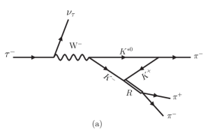
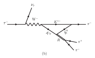
Figure 1: Diagram for the decay of $\tau^{-}\to\nu_{\tau}\pi^{-}\pi^{+}\pi^{-}$. (a) The process $\tau^{-}\to\nu_{\tau}K^{*0}K^{-}$ followed by the $K^{*0}$ decay into $\pi^{-}K^{+}$ and the merging of the $K^{-}K^{+}$ into $f_{0}(980)$; (b) The process $\tau^{-}\to\nu_{\tau}K^{*-}K^{0}$ followed by the $K^{*-}$ decay into $\pi^{-}\bar{K}^{0}$ and the merging of the $K^{0}\bar{K}^{0}$ into $f_{0}(980)$.

Similarly, in Fig. 2, we investigate the $\tau^{-}\to\nu_{\tau}\pi^{-}\pi^{0}\eta$ decay via $a_{0}(980)$ formation, where Fig. 2(a) shows the process $\tau^{-}\to\nu_{\tau}K^{*0}K^{-}$ followed by the $K^{*0}$ decay into $\pi^{-}K^{+}$ and the merging of the $K^{-}K^{+}$ into $a_{0}(980)$, and the process $\tau^{-}\to\nu_{\tau}K^{*-}K^{0}$ followed by the ${K}^{*-}$ decay into $\pi^{-}\bar{K}^{0}$ and the merging of the $K^{0}\bar{K}^{0}$ into $a_{0}(980)$. Both processes also generate a singularity, and we will see a signal for the isospin $I=1$ resonance state $a_{0}(980)$ in the invariant mass of $\pi^{0}\eta$. In the study of Refs. [35, 36, 37, 38, 39], the $a_{0}(980)$ appears as the dynamically generated state of $K^{+}K^{-}$, $K^{0}\bar{K}^{0}$, and $\pi^{0}\eta$ in the coupled-channels calculation. The momenta assignment for the decay process is given in Fig. 3.

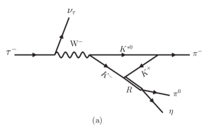
Figure 2: Diagram for the decay of $\tau^{-}\to\nu_{\tau}\pi^{-}\pi^{0}\eta$. (a) The process $\tau^{-}\to\nu_{\tau}K^{*0}K^{-}$ followed by the $K^{*0}$ decay into $\pi^{-}K^{+}$ and the merging of the $K^{-}K^{+}$ into $a_{0}(980)$; (b) The process $\tau^{-}\to\nu_{\tau}K^{*-}K^{0}$ followed by the ${K}^{*-}$ decay into $\pi^{-}\bar{K}^{0}$ and the merging of the $K^{0}\bar{K}^{0}$ into $a_{0}(980)$.

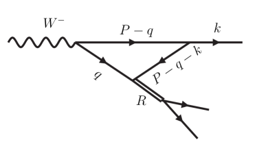
Figure 3: The momenta assignment for the decay process

Let us address, next, the evaluation of the $\tau\to\nu_{\tau}K^{*0}K^{-},\nu_{\tau}K^{*-}K^{0}$ parts. The production is assumed to proceed first from the Cabibbo favored $\bar{u}d$ production from the $W^{-}$ which then hadronizes producing an $s\bar{s}$ with quantum numbers of the vacuum, which are implemented with the ${}^{3}P_{0}$ model [40, 41, 42]. This leads to the $K^{*0}K^{-}$ and $K^{0}K^{*-}$ states with the same weight. In Ref. [30] the mechanism for hadronization is done in detail. The first step corresponds to the flavor combinations in the hadronization. There it is shown that $d(\bar{s}s)\bar{u}=(d\bar{s})s\bar{u}$ gives rise to $K^{0}K^{*-}$ and $K^{*0}K^{-}$ with the same weight (see Eqs. (2) and (3) of Ref. [30]). The second step corresponds to the detailed study of the spin-angular momentum algebra to combine the quarks for the ${}^{3}P_{0}$ $\bar{s}s$ state ($L^{\prime}=1,S^{\prime}=1,J^{\prime}=0$) with a $\bar{d}$ quark in $L=1$ to have finally $s$-wave production of the two mesons. In Ref. [30] the $p$-wave vector-pseudoscalar production was ruled out based on the theoretical results, and experimental results that show the vector-pseudoscalar pairs coupling to axial vector resonance $J^{PC}=1^{++}$[43], which proceeds with $s$-wave. The needed results from [30] are given in the next subsection.

II.1 $\tau\to\nu_{\tau}K^{*0}K^{-}$ decay

The elementary quark interaction is given by

$$H=\mathcal{C}L^{\mu}Q_{\mu}\,,$$ (1)

where $\mathcal{C}$ contains the couplings of the weak interaction. The leptonic current is given by

$$L^{\mu}=\langle{\bar{u}}_{\nu}|\gamma^{\mu}-\gamma^{\mu}\gamma_{5}|u_{\tau}\rangle\,,$$ (2)

and the quark current by

$$Q^{\mu}=\langle\bar{u}_{d}|\gamma^{\mu}-\gamma^{\mu}\gamma_{5}|v_{\bar{u}}\rangle\,.$$ (3)

As is usual in the evaluation of decay widths to three final particles, we evaluate the matrix elements in the frame where the two mesons system is at rest. For the evaluation of the matrix element $Q_{\mu}$ we assume that the quark spinors are at rest in that frame [30], then we have $\gamma^{0}\to 1$, $\gamma^{i}\gamma_{5}\to\sigma^{i}$ in terms of bispinors $\chi$ and after the spin angular momentum combination we have

$$Q_{0} = \langle\chi^{\prime}|1|\chi\rangle\to M_{0}\,,$$

$$Q_{i} = \langle\chi^{\prime}|\sigma_{i}|\chi\rangle\to N_{i}\,.$$ (4)

Denoting for simplicity,

$$\overline{L}^{\mu\nu}=\overline{\sum}\sum L^{\mu}{L^{\nu}}^{\dagger}\,,$$ (5)

to obtain the $\tau$ width we must evaluate

$$\overline{\sum}\sum\left|t\right|^{2} = \overline{\sum}\sum L^{\mu}{L^{\nu}}^{\dagger}Q_{\mu}Q_{\nu}^{*}\,,$$ (6)

$$= \bar{L}^{00}\,M_{0}~{}M^{*}_{0}+\bar{L}^{0i}\,M_{0}~{}N^{*}_{i}+\bar{L}^{i0}\,N_{i}~{}M^{*}_{0}+\bar{L}^{ij}N_{i}~{}N_{j}^{*}\,,$$

with $\overline{L}^{\mu\nu}$ given by

$$\overline{\sum}\sum L^{\mu}{L^{\nu}}^{\dagger}=\frac{1}{m_{\nu}m_{\tau}}\left(p^{\prime\mu}p^{\nu}+p^{\prime\nu}p^{\mu}-g^{\mu\nu}p^{\prime}\cdot p+i\epsilon^{\alpha\mu\beta\nu}p^{\prime}_{\alpha}p_{\beta}\right)\,,$$ (7)

where $p,p^{\prime}$ are the momenta of the $\tau$ and $\nu_{\tau}$ respectively and we use the field normalization for fermions of Ref. [44].

From the work [30] we obtain the results for the $J=1,J^{\prime}=0$ case, which corresponds to the $\tau\to\nu_{\tau}K^{*0}K^{-}$ decay.

$$M_{0} = \frac{1}{\sqrt{6}}\frac{1}{4\pi}\,,~{}~{}~{}~{}~{}{\rm for~{}any~{}~{}}M\,,$$

$$N_{\mu} = (-1)^{-\mu}\frac{1}{\sqrt{3}}\frac{1}{4\pi}{\cal C}(111;M,-\mu,M-\mu)\,,$$ (8)

where $M$ is the third component of $J$ and $\mu$ is the index of $N_{i}$ in spherical basis, with ${\cal C}(\cdots)$ a Clebsch-Gordan coefficient.

It was shown in [30] that the order in which the vector and pseudoscalar mesons are produced is essential to understand the $G$-parity symmetry of these reactions. Then from [30] we write here the results for $PV$ production $J=0,J^{\prime}=1$, which corresponds to the $\tau\to\nu_{\tau}K^{0}K^{*-}$ decay,

$$M_{0} = \frac{1}{\sqrt{6}}\frac{1}{4\pi}\,,~{}~{}~{}~{}~{}{\rm for~{}any~{}~{}}M^{\prime}\,,$$

$$N_{\mu} = -(-1)^{-\mu}\frac{1}{\sqrt{3}}\frac{1}{4\pi}{\cal C}(111;M^{\prime},-\mu,M^{\prime}-\mu)\,.$$ (9)

Note that while $M_{0}$ is the same for $VP$ and $PV$ productions, $N_{i}$ changes sign for $VP$ and $PV$. This sign is essential for the conservation of $G$-parity in the reaction, as we shall see. Indeed, at the quark level the primary $d\bar{u}$ state produced has $I_{3}=-1$ and hence $I=1$. The $G$-parity of a $q\bar{q}$ pair is given by $(-1)^{L+S+I}$. As we mentioned $L=1,I=1$ and the spin of the state is $0$ for the $1$ operator and $1$ for the $\sigma^{i}$ operator of Eq. (II.1). This means that the term $M_{0}$ proceeds with $G$-parity positive, while $N_{i}$ has $G$-parity negative. Since $\pi$, $f_{0}(980)$, and $a_{0}(980)$ have $G$-parity $-,+,-$ respectively, then $\pi^{-}f_{0}(980)$ will proceed with the $N_{i}$ amplitude, while $\pi^{-}a_{0}(980)$ proceeds with the $M_{0}$ term and there is no simultaneous contribution of the two terms in these reactions. This we shall see analytically when evaluating explicitly the amplitudes for the processes of Figs. 1 and 2.

As seen in Eq. (1), we have the unknown constant $\cal{C}$ in our approach which includes factors involving the matrix elements of the radial quark wave functions (the spin-angular momentum variables are explicitly accounted for in the work of [30]). We then determine $\cal{C}$ from the experimental ratio of $\tau\to\nu_{\tau}K^{*0}K^{-}$. For this we use the results of [30] for this reaction.

By taking the quantization axis along the direction of the neutrino in the $\tau^{-}$ rest frame, we find

$$\overline{\sum}\sum\left|t\right|^{2} = \frac{{\cal{C}}^{2}}{m_{\tau}m_{\nu}}\left(\frac{1}{4\pi}\right)^{2}\left[\left(E_{\tau}E_{\nu}+{p}^{2}\right)\frac{1}{2}{h}^{2}_{i}+\left(E_{\tau}E_{\nu}-\frac{1}{3}{p}^{2}\right)\overline{h}^{2}_{i}\right]\,$$ (10)

$$= \frac{{\cal{C}}^{2}}{m_{\tau}m_{\nu}}\left(\frac{1}{4\pi}\right)^{2}\left(\frac{3}{2}E_{\tau}E_{\nu}+\frac{1}{6}{p}^{2}\right)$$

where ${h}_{i}=\overline{h}_{i}=1$, $p$ is the momentum of the $\tau$, or $\nu_{\tau}$, in the $K^{*0}K^{-}$ rest frame, given by

$$p=p_{\nu}=p_{\tau}=\frac{\lambda^{1/2}(m^{2}_{\tau},m^{2}_{\nu},M_{\rm inv}^{2}(K^{*0}K^{-}))}{2M_{\rm inv}{(K^{*0}K^{-})}}\,,$$ (11)

and $E_{\nu}=p$, $E_{\tau}=\sqrt{m_{\tau}^{2}+p^{2}}$.

Now for $\tau\to\nu_{\tau}K^{*0}K^{-}$ decay, we obtain

$$\frac{d\Gamma}{dM_{\rm inv}{(K^{*0}K^{-})}}=\frac{2\,m_{\tau}2\,m_{\nu}}{(2\pi)^{3}}\frac{1}{4m^{2}_{\tau}}\,p^{\prime}_{\nu}{\widetilde{p}_{K}}\,\overline{\sum}\sum\left|t\right|^{2}\,,$$ (12)

where $p^{\prime}_{\nu}$ is the neutrino momentum in the $\tau$ rest frame

$$p^{\prime}_{\nu}=\frac{\lambda^{1/2}(m^{2}_{\tau},m^{2}_{\nu},M_{\rm inv}^{2}(K^{*0}K^{-}))}{2m_{\tau}}\,,$$ (13)

and ${\widetilde{p}_{K}}$ the momentum of $K^{-}$ in the $K^{*0}K^{-}$ rest frame given by

$$\widetilde{p}_{K}=\frac{\lambda^{1/2}(M_{\rm inv}^{2}(K^{*0}K^{-}),m_{K^{*0}}^{2},m_{K^{-}}^{2})}{2M_{\rm inv}{(K^{*0}K^{-})}}\,.$$ (14)

Experimentally, the branching ratio of ${\cal B}(\tau\to\nu_{\tau}K^{*0}K^{-})$ decay,

$${\cal B}(\tau\to\nu_{\tau}K^{*0}K^{-})=\frac{1}{\Gamma_{\tau}}\Gamma(\tau\to\nu_{\tau}K^{*0}K^{-})=(2.1\pm 0.4)\times 10^{-3},$$ (15)

and then

$$\frac{{\cal C}^{2}}{\Gamma_{\tau}}=\frac{{\cal B}(\tau\to\nu_{\tau}K^{*0}K^{-})}{\int_{m_{K^{-}}+m_{K^{*0}}}^{m_{\tau}}\frac{1}{(2\pi)^{3}}\frac{1}{m^{2}_{\tau}}p^{\prime}_{\nu}{\widetilde{p}_{K}}\frac{1}{(4\pi)^{2}}\left(\frac{3}{2}E_{\tau}E_{\nu}+\frac{1}{6}\,{p}^{2}\right)dM_{\rm inv}{(K^{*0}K^{-})}}\,,$$ (16)

from which we can evaluate the value of the constant ${\cal C}^{2}$.

II.2 Evaluation of the triangle diagram

In Eq. (II.1) we need $M$, the third component of $J$. In order to evaluate the loops of Figs.1, 2, we find most convenient to take the $z$ direction along the momentum $\bm{k}$ of the pion produced (see Fig.3). Indeed, in the $\pi f_{0}(980)$ rest frame, where we evaluate the amplitude, ${\bm{P}}=0$. The vertex $K^{*}\to K\pi$ is of the type ${\bm{\epsilon}}\cdot({\bm{k}}+{\bm{q}}+{\bm{k}})$ . The ${\bm{q}}$ integration of $\int d^{3}q~{}q_{i}~{}k_{i}\cdots\cdots$ will necessarily give something proportional to ${\bm{k}}$, which is the only non integrated vector in the loop integral. Hence, we have an effective vertex of the type ${\bm{\epsilon}}\cdot{\bm{k}}$. If the $z$ direction is chosen along ${\bm{k}}$, this selects only the ${\bm{\epsilon}}_{z}$ component (${\bm{\epsilon}}_{0}$ in spherical basis) and ${\bm{\epsilon}}\cdot{\bm{k}}=|{\bm{k}}|=k$. This also means that only $M=0$ contributes in the loop and this allows us to calculate trivially the $M_{0}$, $N_{\mu}$ amplitude in that frame. Indeed for $J=1,J^{\prime}=0$,

$$M_{0} \to \frac{1}{\sqrt{6}}\frac{1}{4\pi}\,,$$

$$N_{\mu} \to (-1)^{-\mu}\frac{1}{\sqrt{3}}\frac{1}{4\pi}{\cal C}(111;0,-\mu,-\mu)\,,$$ (17)

and for $J=0,J^{\prime}=1$, $M_{0}$ is the same and $N_{\mu}$ changes sign.

Explicit calculation of the Clebsch-Gordan coefficients in Eq.(II.2) gives

$$N_{\mu=+1}=-\frac{1}{\sqrt{3}}\frac{1}{4\pi}\frac{1}{\sqrt{2}}\,,\qquad N_{\mu=-1}=\frac{1}{\sqrt{3}}\frac{1}{4\pi}\frac{1}{\sqrt{2}}\,,\qquad N_{\mu=0}=0\,,$$ (18)

which in cartesian coordinate can be written as

$$N_{i}=\frac{1}{\sqrt{3}}\frac{1}{4\pi}\delta_{i1}\,,$$ (19)

the index $1$ for the $x$ direction. We now define the triangle loop functions, $t_{L}$, such that

$$t_{L}gt_{K^{+}K^{-},\pi^{+}\pi^{-}}{\bm{k}} = i\int\frac{d^{4}q}{(2\pi)^{4}}\frac{1}{q^{2}-m^{2}_{k^{-}}+i\epsilon}\frac{1}{(P-q)^{2}-m^{2}_{K^{*0}}+i\epsilon}\,,$$ (20)

$$\times \frac{1}{(P-q-k)^{2}-m_{K^{+}}^{2}+i\epsilon}\,g\,(2{\bm{k}}+{\bm{q}})\,t_{K^{+}K^{-},\pi^{+}\pi^{-}}\,,$$

where the $K^{*0}\to\pi^{-}K^{+}$ vertex has been evaluated from the $VPP$ Lagrangian

$$\mathcal{L}_{VPP}=-ig\left<V^{\mu}\left[P,\partial_{\mu}P\right]\right>\,,$$ (21)

and the brackets $\left<...\right>$ mean the trace over the SU(3) flavour matrices, with the coupling $g$ given by $g=m_{V}/2f_{\pi}$ in the local hidden gauge approach, with $m_{V}=800\ \text{MeV}$ and $f_{\pi}$=93 MeV.

As mentioned above,

$$\int f({\bm{k}},{\bm{q}})q^{i}=Ak^{i}\,,\qquad A=\int f({\bm{k}},{\bm{q}})\frac{\bm{q}\cdot\bm{k}}{|\bm{k}|^{2}}\,,$$ (22)

Hence, ${\bm{q}}$ in $2{\bm{k}}+{\bm{q}}$ in Eq. (20) can be replaced effectively by $\frac{\bm{q}\cdot\bm{k}}{|\bm{k}|^{2}}{\bm{k}}$. By performing analytically the $q^{0}$ integration in Eq. (20) we find [45, 46]

$$t_{T}= \int\frac{d^{3}q}{(2\pi)^{3}}\frac{1}{8\omega_{K^{*}}\omega_{K^{+}}\omega_{K^{-}}}\frac{1}{k^{0}-\omega_{K^{+}}-\omega_{K^{*}}+i\frac{\Gamma_{K^{*}}}{2}}\frac{1}{P^{0}+\omega_{K^{-}}+\omega_{K^{+}}-k^{0}}\left(2+\frac{\bm{q}\cdot\bm{k}}{|\bm{k}|^{2}}\right)\,$$

$$\times\frac{1}{P^{0}-\omega_{K^{-}}-\omega_{K^{+}}-k^{0}+i\epsilon}\frac{2P^{0}\omega_{K^{-}}+2k^{0}\omega_{K^{+}}-2(\omega_{K^{-}}+\omega_{K^{+}})(\omega_{K^{-}}+\omega_{K^{+}}+\omega_{K^{*}})}{P^{0}-\omega_{K^{*}}-\omega_{K^{-}}+i\frac{\Gamma_{K^{*}}}{2}},$$ (23)

with $P^{0}=M_{\rm inv}(\pi^{-}f_{0})$, $\omega_{K^{-}}=\sqrt{\bm{q}^{2}+m_{K}^{2}}$, $\omega_{K^{+}}=\sqrt{({\bm{q}}+{\bm{k}})^{2}+m_{K}^{2}}$, and $\omega_{K^{*}}=\sqrt{\bm{q}^{2}+m_{K^{\ast}}^{2}}$

$$k^{0}=\frac{M^{2}_{\rm inv}(\pi^{-}f_{0})+m_{\pi}^{2}-M^{2}_{\rm inv}(\pi^{+}\pi^{-})}{2M_{\rm inv}(\pi^{-}f_{0})},$$ (24)

$$k=\frac{\lambda^{1/2}(M^{2}_{\rm inv}(\pi^{-}f_{0}),m_{\pi}^{2},M^{2}_{\rm inv}(\pi^{+}\pi^{-}))}{2M_{\rm inv}(\pi^{-}f_{0})}.$$ (25)

Similarly, we can get the triangle amplitude for the $\pi^{-}a_{0}$ case. Note also that an $i\epsilon$ in the propagators involving $\omega_{K^{*}}$ is replaced by $i\frac{\Gamma_{K^{*}}}{2}$.

Then the formalism for the loop diagrams can be done as for the $K^{*0}K^{-}$ production replacing

$$M_{0}\to\widetilde{M}_{0}t_{K^{+}K^{-},\pi^{+}\pi^{-}}\,;\quad\widetilde{M}_{0}=g\frac{1}{\sqrt{6}}\frac{1}{4\pi}\,k\,t_{L}\,,$$

$$N_{i}\to\widetilde{N}_{i}t_{K^{+}K^{-},\pi^{+}\pi^{-}}\,;\quad\widetilde{N}_{i}=g\frac{1}{\sqrt{3}}\frac{1}{4\pi}\,k\,t_{L}\,\delta_{i1}\,$$ (26)

and for $K^{0}K^{*-}$, $\widetilde{M}_{0}$ is the same and $\widetilde{N}_{i}$ changes sign.

The combination of the diagram of Fig. 1(b) proceeds in a similar way. The changes are: $t_{K^{+}K^{-}\to\pi^{+}\pi^{-}}$ is replaced by $t_{K^{0}\bar{K}^{0}\to\pi^{+}\pi^{-}}$ and the $K^{*-}\to\pi^{-}\bar{K}^{0}$ vertex has opposite sign to $K^{*0}\to\pi^{-}K^{+}$. Then, the sum of the two terms is taken into account by means of

$$M_{0} \to \widetilde{M}_{0}(K^{*0}K^{-})\,t_{K^{+}K^{-},\pi^{+}\pi^{-}}-\widetilde{M}_{0}(K^{*-}K^{0})\,t_{K^{0}\bar{K}^{0},\pi^{+}\pi^{-}}\,$$ (27)

$$= \widetilde{M}_{0}(K^{*0}K^{-})\left(t_{K^{+}K^{-},\pi^{+}\pi^{-}}-t_{K^{0}\bar{K}^{0},\pi^{+}\pi^{-}}\right)\,,$$

$$N_{i} \to \widetilde{N}_{i}(K^{*0}K^{-})\,t_{K^{+}K^{-},\pi^{+}\pi^{-}}-\widetilde{N}_{i}(K^{*-}K^{0})\,t_{K^{0}\bar{K}^{0},\pi^{+}\pi^{-}}\,$$ (28)

$$= \widetilde{N}_{i}(K^{*0}K^{-})\left(t_{K^{+}K^{-},\pi^{+}\pi^{-}}+t_{K^{0}\bar{K}^{0},\pi^{+}\pi^{-}}\right)\,.$$

When we have $\pi^{0}\eta$ production, as in Fig. 2, the formalism is identical, we only replace $\pi^{+}\pi^{-}$ by $\pi^{0}\eta$ at the end in $t_{K\bar{K}\to m^{\prime}_{1}m^{\prime}_{2}}$. Next, in order to have isospin conservation and hence proper $G$-parity state we will solve the $t_{m_{1}m_{2}\to m^{\prime}_{1}m^{\prime}_{2}}$ amplitudes with average masses for the kaons and average masses for the pions and we shall also take average masses for $K^{*}$ masses in the loop. In this case we have

$$t_{K^{+}K^{-},\pi^{+}\pi^{-}} = t_{K^{0}\bar{K}^{0},\pi^{+}\pi^{-}}\,,$$

$$t_{K^{+}K^{-},\pi^{0}\eta~{}} = -t_{K^{0}\bar{K}^{0},\pi^{0}\eta~{}}\,.$$ (29)

Hence in the case of the amplitude $M_{0}$ in Eq. (27) and $\pi^{+}\pi^{-}$ in the final state we find a cancellation of the amplitudes for diagram of Figs. 1 (a) and 1 (b). If instead we have $\pi^{0}\eta$ in the end, the two diagrams of Figs. 2 (a) and 2 (b) give the same contribution and sum coherently. Conversely, in the $N_{i}$ term of Eq. (28) the two terms corresponding to Figs. 1 (a) and 1 (b) add and those of Figs. 2 (a) and 2 (b) cancel exactly. In summary, the $M_{0}$ terms cancel for the production of $f_{0}(980)$ and add for the production of $a_{0}(980)$. This is, the $f_{0}(980)$ production proceeds via the $N_{i}$ term and the $a_{0}(980)$ production via the $M_{0}$ term. Since $\pi^{-}f_{0}(980)$ has negative $G$-parity and $\pi^{-}a_{0}(980)$ positive $G$-parity, we confirm that the $M_{0}$ term in the loop corresponds to positive $G$-parity and the $N_{i}$ term to negative $G$-parity, as we found earlier at the quark level.

Then for $\pi^{-}f_{0}(980)$ we will have

$$\overline{\sum}\sum\left|t\right|^{2} = \bar{L}^{ij}\widetilde{N}_{i}~{}\widetilde{N}_{j}^{*}\,g^{2}\,|\,2\,t_{K^{+}K^{-},\pi^{+}\pi^{-}}|^{2}\,,$$ (30)

$$= \frac{{\cal C}^{2}}{m_{\tau}m_{\nu}}\left(E_{\tau}E_{\nu}-\frac{1}{3}p^{2}\right)\frac{1}{3}\frac{1}{(4\pi)^{2}}\,k^{2}|t_{L}|^{2}\,g^{2}\,|\,2\,t_{K^{+}K^{-},\pi^{+}\pi^{-}}|^{2}\,.$$

Similarly, for the production of $\pi^{-}a_{0}(980)$ we will have

$$\overline{\sum}\sum\left|t\right|^{2} = \bar{L}^{00}\widetilde{M}_{0}~{}\widetilde{M}_{0}^{*}\,g^{2}\,|\,2\,t_{K^{+}K^{-},\pi^{0}\eta}|^{2}\,,$$ (31)

$$= \frac{{\cal C}^{2}}{m_{\tau}m_{\nu}}\left(E_{\tau}E_{\nu}+p^{2}\right)\frac{1}{6}\frac{1}{(4\pi)^{2}}\,k^{2}|t_{L}|^{2}\,g^{2}\,|\,2\,t_{K^{+}K^{-},\pi^{0}\eta}|^{2}\,.$$

where we have taken into account that $p_{i}\delta_{i1}p_{j}\delta_{j1}$ is $p^{2}_{x}$ and when integrated over the phase space gives rise to $\frac{1}{3}p^{2}$.

For $\tau^{-}\to\nu_{\tau}\pi^{-}\pi^{+}\pi^{-}$ decay, the double differential mass distribution for $M_{\rm inv}(\pi^{+}\pi^{-})$ and $M_{\rm inv}(\pi^{-}f_{0})$ is given by [16]

$$\frac{1}{\Gamma_{\tau}}\frac{d^{2}\Gamma}{dM_{\text{inv}}(\pi^{-}f_{0})dM_{\text{inv}}(\pi^{+}\pi^{-})}=\frac{1}{(2\pi)^{5}}\frac{1}{\Gamma_{\tau}}k\,p^{\prime}_{\nu}\,\widetilde{q}_{\pi^{+}}\,\frac{2m_{\tau}2m_{\nu}}{4M^{2}_{\tau}}\overline{\sum}\sum\left|t\right|^{2}\,,$$ (32)

with $k$ given by Eq.(25) and

$$p^{\prime}_{\nu}=\frac{\lambda^{1/2}(m_{\tau}^{2},m^{2}_{\nu},M^{2}_{\text{inv}}(\pi^{-}f_{0}))}{2m_{\tau}},\quad\widetilde{q}_{\pi^{+}}=\frac{\lambda^{1/2}(M^{2}_{\text{inv}}(\pi^{+}\pi^{-}),m^{2}_{\pi},m^{2}_{\pi})}{2M_{\text{inv}}(\pi^{+}\pi^{-})}.$$ (33)

Similarly, for the $\tau^{-}\to\nu_{\tau}\pi^{-}\pi^{0}\eta$ decay, we can get the double differential mass distribution for $M_{\rm inv}(\pi^{0}\eta)$ and $M_{\rm inv}(\pi^{-}a_{0})$.

Note that the term ${m_{\tau}m_{\nu}}$ in the numerator of Eq.(32) cancels the same factor in the denominator of Eqs. (30) and (31). In Eq.(32) we have the factor $\frac{{\cal C}^{2}}{\Gamma_{\tau}}$, which, as mentioned before, is obtained by means of Eq.(16), and thus we can provide absolute values for the mass distributions.

III Results

Let us begin by showing in Fig. 4 the contribution of the triangle loop defined in Eq. (II.2). We plot the real and imaginary parts of $t_{L}$, as well as the absolute value as a function of $M_{\rm inv}(\pi^{-}R)$, with $M_{\rm inv}(R)$ fixed at $985$ MeV ($R$ standing for $f_{0}(980)$ or $a_{0}(980)$). It can be observed that ${\rm Re}(t_{T})$ has a peak around $1393$ MeV, and ${\rm Im}(t_{T})$ has a peak around $1454$ MeV, and there is a peak for $|t_{T}|$ around 1425 MeV. As discussed in Refs. [18, 11], the peak of the real part is related to the $K^{*}K$ threshold and the one of the imaginary part, that dominates for the larger $\pi^{-}R$ invariant masses, to the triangle singularity. Note that around $1420$ MeV and above the triangle singularity dominates the reaction.

The origin of the peak in $|t_{T}|$ and consequently in the $\pi^{-}R$ mass distribution of the decay has then the same origin as the peak observed in the COMPASS experiment [6], tentatively branded as a new “$a_{1}(1420)$” resonance, which however was explained in [3, 4] as coming from the same triangle mechanism that we have encountered here. It would be most enlightening to confirm this experimentally in the $\tau$ decay reaction to settle discussions around the “$a_{1}(1420)$” peak.

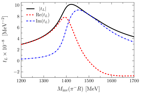
Figure 4: Triangle amplitude ${\rm Re}(t_{L})$, ${\rm Im}(t_{L})$ and $|t_{L}|$, taking $M_{\rm inv}(R)$=985 MeV

In Fig. 5 we plot Eq.(32) for the $\tau^{-}\to\nu_{\tau}\pi^{-}\pi^{+}\pi^{-}$ decay, and similarly in Fig.6 for the $\tau^{-}\to\nu_{\tau}\pi^{-}\pi^{0}\eta$ decay as a function of $M_{\rm inv}(R)$, where in both figures we fix $M_{\rm inv}(\pi^{-}R)$=1317 MeV, 1417 MeV, and 1517 MeV and vary $M_{\rm inv}(R)$. We can see that the distribution with largest strength is near $M_{\rm inv}(\pi^{-}R)$=1417 MeV. In Fig.5 we can also see a strong peak in the $\pi^{+}\pi^{-}$ mass distribution around $980$ MeV for the three different masses of $M_{\rm inv}(\pi^{-}R)$, corresponding to the $f_{0}(980)$. Similarly, in Fig.6 we see the distinctive cusp like $a_{0}(980)$ peak around $990$ MeV for the $\pi^{0}\eta$ mass distribution. Consequently, we see that most of the contribution to the width $\Gamma$ comes from $M_{\rm inv}(R)=M_{R}$ (the nominal mass of the $f_{0}$ or $a_{0}$ resonance), and we have strong contributions for $M_{\rm inv}(\pi^{+}\pi^{-})\in[950~{}\rm{MeV},1000~{}\rm{MeV}]$ and $M_{\rm inv}(\pi^{0}\eta)\in[900~{}\rm{MeV},1050~{}\rm{MeV}]$. Therefore, when we calculate the mass distribution $\frac{d\Gamma}{dM_{\rm inv}(\pi^{-}R)}$, we restrict the integral to the limits already mentioned.

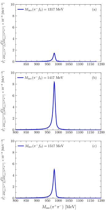
Figure 5: Double differential width of $\tau^{-}\to\nu_{\tau}\pi^{-}\pi^{+}\pi^{-}$, keeping $M_{\rm inv}(\pi^{-}f_{0})$ fixed to three values. Lines (a),(b) and (c) show the values at $M_{\rm inv}(\pi^{-}f_{0})$ 1317 MeV, 1417 MeV, and 1517 MeV, respectively, plotted versus $M_{\rm inv}(\pi^{+}\pi^{-})$.

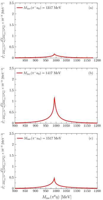
Figure 6: Double differential width of $\tau^{-}\to\nu_{\tau}\pi^{-}\pi^{0}\eta$, keeping $M_{\rm inv}(\pi^{-}a_{0})$ fixed to three values. Lines (a),(b) and (c) show the values at $M_{\rm inv}(\pi^{-}a_{0})$ 1317 MeV, 1417 MeV, and 1517 MeV, respectively, plotted versus $M_{\rm inv}(\pi^{0}\eta)$.

By integrating over $M_{\rm inv}(R)$, we obtain $\frac{1}{\Gamma_{\tau}}\frac{d\Gamma}{dM_{\rm inv}(\pi^{-}R)}$ which is shown in Fig. 7. We see a clear peak of the distribution around $1423$ MeV for $\pi^{-}f_{0}(980)$ production and $1412$ MeV for $\pi^{-}a_{0}(980)$ production. Integrating $\frac{d\Gamma}{dM_{\rm inv}(\pi^{-}R)}$ over $M_{\rm inv}(\pi^{-}R)$ in Fig. 7, we obtain the branching fractions

$${\cal B}(\tau\to\nu_{\tau}\pi^{-}f_{0}(980);~{}~{}f_{0}(980)\rightarrow\pi^{+}\pi^{-}) = (2.6\pm 0.5)\times 10^{-4}\,,$$

$${\cal B}(\tau\to\nu_{\tau}\pi^{-}a_{0}(980);~{}~{}a_{0}(980)\rightarrow\pi^{0}\eta) = (7.1\pm 1.4)\times 10^{-5}\,.$$ (34)

Since the rate of $f_{0}\to\pi^{0}\pi^{0}$ is one half that of $f_{0}\to\pi^{+}\pi^{-}$, we can write

$${\cal B}(\tau\to\nu_{\tau}\pi^{-}f_{0}(980);~{}~{}f_{0}(980)\rightarrow\pi^{+}\pi^{-}) = (3.9\pm 0.8)\times 10^{-4}\,.$$ (35)

The errors in these numbers count only the relative error of the branching ratio of Eq. (15). These numbers are within measurable range, since branching ratios of $10^{-5}$ and smaller are quoted in the PDG for $\tau$ decays [7].

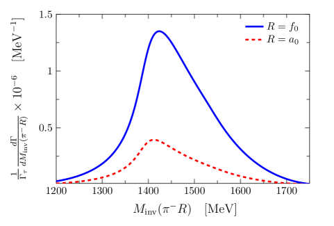
Figure 7: The mass distribution for $\pi^{-}R$ ($R=f_{0},a_{0}$). The solid line for $\tau^{-}\to\nu_{\tau}\pi^{-}\pi^{+}\pi^{-}$ as a function of $M_{\rm inv}(\pi^{-}R)$ with $R\equiv f_{0}(980)$ measured in the $\pi^{+}\pi^{-}$ decay mode; dashed line for $\tau^{-}\to\nu_{\tau}\pi^{-}\pi^{0}\eta$ as a function of $M_{\rm inv}(\pi^{-}R)$ with $R\equiv a_{0}(980)$ measured in the $\pi^{0}\eta$ decay mode.

IV Conclusions

We have made a study of the $\tau^{-}\to\nu_{\tau}\pi^{-}f_{0}(980)$ and $\tau^{-}\to\nu_{\tau}\pi^{-}a_{0}(980)$ reactions from the perspective that the $f_{0}(980)$ and $a_{0}(980)$ are dynamically generated resonances from the interaction of pseudoscalar mesons in coupled channnels. We showed that the formalism for these processes proceeds via $\tau\to\nu_{\tau}K^{*0}K^{-}$ ($K^{0}K^{*-}$) followed by $\bar{K}^{*}\to\pi^{-}K$ and the posterior fusion of $K\bar{K}$ to produce either the $f_{0}(980)$ or $a_{0}(980)$ states. This triangle mechanism has a peculiarity since it develops a triangle singularity at $M_{\rm inv}(\pi^{-}R)\simeq 1420$ MeV ($R\equiv f_{0}$ or $a_{0}$), and the $M_{\rm inv}(\pi^{-}R)$ distribution shows a peak around this energy, which has then the same origin as the explanations given in [3, 4] for the COMPASS peak in $\pi f_{0}(980)$ that was initially presented as the new resonance “$a_{1}(1420)$”. It would be most instructive to have the experiment performed to see if such peak indeed appears, which would help clarify the issue around the “$a_{1}(1420)$” peak.

On the other hand we make predictions which are tied to the way the $f_{0}(980)$ and $a_{0}(980)$ resonances are generated and again the observations will bring extra information on the nature of these low-lying scalar states.

The mechanism requires the use of the amplitude for $\tau\to\nu_{\tau}K^{*0}K^{-}$ reaction in a way suited to the calculation of the loop function of the triangle mechanism. This task was made efficient and easily manageable thanks to the formalism developed in [30] which provides two amplitudes with given $G$-parity in terms of the third components of the $K^{*0}$ spin. Since $\pi^{-}f_{0}(980)$ and $\pi^{-}a_{0}(980)$ have negative and positive $G$-parity respectively, the formalism filtered just one of these amplitudes for either reaction, with the subsequent economy and clarity in the formulation.

We could provide absolute values for the mass distributions and final branching ratios by using the experimental branching ratio of the $\tau\to\nu_{\tau}K^{*0}K^{-}$ reaction. Hence, our predictions are free of intrinsic uncertainties that ab initio microscopic models unavoidably have, and which would be magnified in this problem where final state interaction of hadrons is at work.

With the reliable predictions of our approach we find final branching ratios of $\pi^{-}f_{0}(980)$ and $\pi^{-}a_{0}(980)$ of about $4\times 10^{-4}$ and $7\times 10^{-5}$, respectively. These rates are well within measurable range and we can only encourage the performance of the experiments. Actually some partial information already exists for the reactions, exposed in [47] where the reaction $\tau^{-}\to\nu_{\tau}\pi^{-}\pi^{0}\eta$ is measured, with a branching ratio $1.38\times 10^{-3}$, but the $\pi^{0}\eta\to a_{0}(980)$ mode is not isolated, In [48] this reaction is also measured and a peak seems to be present around $M_{\rm inv}(\pi^{-}\pi^{0}\eta)\simeq 1420$ MeV, but since the $\pi^{0}\eta\to a_{0}(980)$ channel is not isolated we can not conclude that this corresponds to $\pi^{-}a_{0}(980)$. The same can be said about the work of [49] where a peak around $1450$ MeV seems to be present in the $\pi^{-}\pi^{0}\eta$ invariant mass. As for $\pi^{-}\pi^{+}\pi^{-}$ there are also studies in [50, 51, 52] but no mass distributions are available. If the idea of building a $\tau$ facility in China prospers, the suggestion of new decay modes and predictions like those in the present work will be most opportune to make such facility really useful. Meanwhile, the experiments just quoted, with larger statistic, could produce new results to test our predictions.

References

- [1] L. D. Landau, Nucl. Phys. 13, 181 (1959).
- [2] S. Coleman and R. E. Norton, Nuovo Cim. 38, 438 (1965).
- [3] M. Mikhasenko, B. Ketzer and A. Sarantsev, Phys. Rev. D 91, 094015 (2015).
- [4] F. Aceti, L. R. Dai and E. Oset, Phys. Rev. D 94, 096015 (2016).
- [5] X. H. Liu, M. Oka and Q. Zhao, Phys. Lett. B 753, 297 (2016).
- [6] C. Adolph et al. (COMPASS Collaboration), Observation of a New Narrow Axial-Vector Meson , Phys. Rev. Lett. 115, 082001 (2015).
- [7] M. Tanabashi et al. (Particle Data Group), Phys. Rev. D 98, 030001 (2018).
- [8] D. Barberis et al. [WA102 Collaboration], Phys. Lett. B 440, 225 (1998).
- [9] V. R. Debastiani, F. Aceti, W. H. Liang and E. Oset, Phys. Rev. D 95, 034015 (2017).
- [10] J. J. Xie, L. S. Geng and E. Oset, Phys. Rev. D 95, 034004 (2017).
- [11] L. R. Dai, R. Pavao, S. Sakai and E. Oset, Phys. Rev. D 97, 116004 (2018).
- [12] A. P. Szczepaniak, Phys. Lett. B 747, 410 (2015).
- [13] A. P. Szczepaniak, Phys. Lett. B 757, 61 (2016).
- [14] A. E. Bondar and M. B. Voloshin, Phys. Rev. D 93 094008, (2016).
- [15] A. Pilloni et al. [JPAC Collaboration], Phys. Lett. B 772, 200 (2017).
- [16] R. Pavao, S. Sakai and E. Oset, Eur. Phys. J. C 77, 599 (2017).
- [17] X. H. Liu and U. G. Meißner, Eur. Phys. J. C 77, 816 (2017).
- [18] S. Sakai, E. Oset and A. Ramos, Eur. Phys. J. A 54, 10 (2018).
- [19] L. Roca and E. Oset, Phys. Rev. C 95, 065211 (2017).
- [20] D. Samart, W. H. Liang and E. Oset, Phys. Rev. C 96, 035202 (2017).
- [21] J. J. Wu, X. H. Liu, Q. Zhao and B. S. Zou, Phys. Rev. Lett. 108, 081803 (2012).
- [22] F. Aceti, W. H. Liang, E. Oset, J. J. Wu and B. S. Zou, Phys. Rev. D 86, 114007 (2012).
- [23] X. G. Wu, J. J. Wu, Q. Zhao and B. S. Zou, Phys. Rev. D 87, 014023 (2013).
- [24] X. H. Liu and G. Li, Eur. Phys. J. C 76, 455 (2016).
- [25] E. Wang, J. J. Xie, W. H. Liang, F. K. Guo and E. Oset, Phys. Rev. C 95, 015205 (2017).
- [26] J. J. Xie and F. K. Guo, Phys. Lett. B 774, 108 (2017).
- [27] Z. Cao, Q. Zhao, arXiv:1711.07309 [hep-ph].
- [28] W. H. Liang, S. Sakai, J. J. Xie and E. Oset, Chin. Phys. C 42, 044101 (2018).
- [29] V. R. Debastiani, S. Sakai and E. Oset, arXiv:1809.06890 [hep-ph].
- [30] L. R. Dai, R. Pavao, S. Sakai and E. Oset, arXiv:1805.04573 [hep-ph].
- [31] E. Oset and L. Roca, Phys. Lett. B 782, 332 (2018).
- [32] L. Roca, E. Oset and J. Singh, Phys. Rev. D 72 014002, (2005).
- [33] Y. Zhou, X. L. Ren, H. X. Chen and L. S. Geng, Phys. Rev. D 90, 014020 (2014).
- [34] M. K. Volkov, A. A. Pivovarov and A. A. Osipov, Eur. Phys. J. A 54, 61 (2018).
- [35] J. A. Oller and E. Oset, Nucl. Phys. A 620, 438 (1997); A 652, 407 (E) (1999).
- [36] J. Nieves and E. Ruiz Arriola, Nucl. Phys. A 679, 57 (2000).
- [37] N. Kaiser, Eur. Phys. J. A 3, 307 (1998).
- [38] J. J. Xie, L. R. Dai and E. Oset, Phys. Lett. B 742, 363 (2015).
- [39] M. P. Locher, V. E. Markushin and H. Q. Zheng, Eur. Phys. J. C 4, 317 (1998).
- [40] L. Micu, Nucl. Phys. B 10, 521 (1969).
- [41] A. Le Yaouanc, L. Oliver, O. Pène and J. C. Raynal, Phys. Rev. D 8, 2223 (1973).
- [42] E. Santopinto and R. Bijker, Phys. Rev. C 82, 062202 (2010).
- [43] B. C. Barish, R. Stroynowski, Phys. Rept. 157, 1 (1988).
- [44] F. Mandl and G. Shaw, Quantum Field Theory, John Wiley & Sons, 1984.
- [45] F. Aceti, J. M. Dias and E. Oset, Eur. Phys. J. A 51, 48 (2015).
- [46] M. Bayar, F. Aceti, F. K. Guo and E. Oset, Phys. Rev. D 94, 074039 (2016).
- [47] K. Inami et al. [Belle Collaboration], Phys. Lett. B 672, 209 (2009).
- [48] D. Buskulic et al. [ALEPH Collaboration], Z. Phys. C 74, 263 (1997).
- [49] M. Artuso et al. [CLEO Collaboration], Phys. Rev. Lett. 69, 3278 (1992).
- [50] B. Aubert et al. [BaBar Collaboration], Phys. Rev. Lett. 100, 011801 (2008).
- [51] M. J. Lee et al. [Belle Collaboration], Phys. Rev. D 81, 113007 (2010).
- [52] R. A. Briere et al. [CLEO Collaboration], Phys. Rev. Lett. 90, 181802 (2003).