High-Order Isogeometric Methods for Compressible Flows.

Abstract

Isogeometric analysis was applied very successfully to many problem classes like linear elasticity, heat transfer and incompressible flow problems but its application to compressible flows is very rare. However, its ability to accurately represent complex geometries used in industrial applications makes IGA a suitable tool for the analysis of compressible flow problems that require the accurate resolution of boundary layers. The convection-diffusion solver presented in this chapter, is an indispensable step on the way to developing a compressible solver for complex viscous industrial flows. It is well known that the standard Galerkin finite element method and its isogeometric counterpart suffer from spurious oscillatory behaviour in the presence of shocks and steep solution gradients. As a remedy, the algebraic flux correction paradigm is generalized to B-Spline basis functions to suppress the creation of oscillations and occurrence of non-physical values in the solution. This work provides early results for scalar conservation laws and lays the foundation for extending this approach to the compressible Euler equations in igaAFC2_fef2017 .

1 Introduction

Isogeometric analysis (IGA) was proposed by Hughes et al. in IGAArticle . Since its birth it was successfully applied in a variety of use case scenarios ranging from linear elasticity and incompressible flows to fluid-structure interaction problems IGABook . There were, however, not many approaches to apply this method to compressible flow problems IGAart2 ; Jaeschke . Although this application did not gain the attention of many researches yet, it seems to be a promising field. Flow problems are usually defined on domains with complex but smooth shapes, whereby the exact representation of the boundary is indispensable due to the crucial influence of boundary layers on the flow behaviour. This is where IGA has the potential to demonstrate its strengths.

It is a well know fact that standard Galerkin finite element schemes (FEM) suffer from infamous instabilities when applied to convection-dominated problems, such as compressible flows. The same unwanted behaviour occurs for IGA-based standard Galerkin schemes IGABook making it necessary to develop high-resolution high-order isogeometric schemes that overcome these limitations. From the many available approaches including the most commonly used ones, i.e., the streamline upwind Petrov–Galerkin (SUPG) method introduced by Brooks and Hughes in Brooks1982199 , we have chosen for the algebraic flux correction (AFC) methodology, which was introduced by Kuzmin and Turek in Kuzmin2002525 and refined in a series of publications Kuzmin2004131 ; KBOI ; Kuzmin2006513 ; KuzminArticle ; Kuzmin2010 ; KBNI ; KBNII . The family of AFC schemes is designed with the overall goal to prevent the creation of spurious oscillations by modifying the system matrix stemming from a standard Galerkin method in mass-conservative fashion. This algebraic design principle makes them particularly attractive for use in high-order isogeometric methods.

2 High-resolution isogeometric analysis

This section briefly describes the basic construction principles of high-resolution isogeometric schemes for convection-dominated problems based on an extension of the AFC paradigm to B-Spline based discretizations of higher order.

2.1 Model problem

Consider the stationary convection-diffusion problem IGABook

$$-d\Delta u(\mathbf{x}))+\nabla\cdot(\mathbf{v}u(\mathbf{x})) =0 \text{in}\;\Omega$$ (1)

$$u(\mathbf{x}) =\beta(\mathbf{x}) \text{on}\;\varGamma$$ (2)

with diffusion coefficient $d=0.0001$ and constant velocity vector $\mathbf{v}=[\sqrt{2},\sqrt{2}]^{\top}$. The problem is solved on the two domains depicted in Figure 1.

Starting from the open knot vector $\Xi=[0,\,0,\,0,\,0.5,\,1,\,1,\,1]$, quadratic B-Spline basis functions $N_{a,2}(\xi)$ are generated by the Cox-de-Boor recursion formula deBoor1971 :

$$p=0:\quad N_{a,0}(\xi) = \left\{\begin{array}[]{ll}1&\text{if }\xi_{a}\leq\xi<\xi_{a+1},\\ 0&\text{otherwise},\end{array}\right.$$ (5)

$$p>0:\quad N_{a,p}(\xi) = \frac{\xi-\xi_{a}}{\xi_{a+p}-\xi_{a}}N_{a,p-1}(\xi)+\frac{\xi_{a+p+1}-\xi}{\xi_{a+p+1}-\xi_{a+1}}N_{a+1,p-1}(\xi),$$ (6)

where $\xi_{a}$ are the entries in the knot vector $\Xi$. Their tensor product construction yields the bivariate B-Spline basis functions $\hat{\varphi}_{j}(\xi,\eta)=N_{a}(\xi)N_{b}(\eta)$ (with index map $j\mapsto(a,b)$), which are used to define the computational geometry model

$$\mathbf{x}(\xi,\eta)=\sum_{j}\mathbf{c}_{j}\hat{\varphi}_{j}(\xi,\eta),\quad(\xi,\eta)\in\hat{\Omega}=[0,1]^{2}$$ (7)

with control points $\mathbf{c}_{j}\in\mathbb{R}^{2}$ indicated by dots in Fig. 1. The mapping $\phi:\hat{\Omega}\to\Omega$ converts parametric values $\bm{\xi}=(\xi,\eta)$ into physical coordinates $\mathbf{x}=(x,y)$. The mapping should be bijective in order to possess a valid ’pull-back’ operator $\phi^{-1}:\Omega\to\hat{\Omega}$.

For simplicity the boundary conditions are prescribed in the parametric domain:

$$\beta(\mathbf{x}=\phi(\bm{\xi}))=\begin{cases}1&\quad\text{if }\eta\leq\frac{1}{5}-\frac{1}{5}\xi\\ 0&\quad\text{otherwise}.\end{cases}$$ (8)

Figure 1: Unit square (left) and deformed domain (right) modeled by tensor-product quadratic B-Spline basis functions defined on the open knot vector $\Xi=[0,\,0,\,0,\,0.5,\,1,\,1,\,1]$.

2.2 Galerkin method

Application of the Galerkin method to (1)–(8) yields: Find $u^{h}\in S^{h}$ such that

$$d\int_{\Omega}\nabla u^{h}\cdot\nabla v^{h}\mathrm{d}\mathbf{x}+\int_{\Omega}\nabla\cdot(\mathbf{{v}}u)^{h}v^{h})\mathrm{d}\mathbf{x}=\int_{\Omega}Rv^{h}\mathrm{d}\mathbf{x}$$ (9)

for all test functions $v^{h}\in V^{h}$ that vanish on the entire boundary $\Gamma$ due to the prescription of Dirichlet boundary conditions. In the framework of IGA the discrete spaces $S^{h}$ and $V^{h}$ are spanned by multivariate B-Spline basis functions $\{\varphi_{j}(\mathbf{x})\}$.

Using Fletcher’s group formulation Fletcher , the approximate solution $u^{h}$ and the convective flux $(\mathbf{{v}}u)^{h}$ can be represented as follows KBNI :

$$u^{h}(\mathbf{x})=\sum_{j}u_{j}\varphi_{j}(\mathbf{x}),\quad(\mathbf{{v}}u)^{h}(\mathbf{x})=\sum_{j}(\mathbf{{v}}_{j}u_{j})\varphi_{j}(\mathbf{x}).$$ (10)

Substitution into (9) and replacing $v^{h}$ by all basis functions yields the matrix form

$$(S-K)\mathbf{u}=\mathbf{r},$$ (11)

where $\mathbf{u}$ is the vector of coefficients $u_{i}$ used in the expansion of the solution (10) and the entries of the discrete diffusion ($S=\{s_{ij}\}$) and convection ($K=\{k_{ij}\}$) operators and the discretized right-hand side vector ($\mathbf{r}=\{r_{i}\}$) are given by

$$k_{ij} =-\mathbf{v}_{j}\cdot\mathbf{c}_{ij}, \mathbf{c}_{ij} =\int_{\Omega}\nabla\varphi_{j}\varphi_{i}\mathrm{d}\mathbf{x},$$ (12)

$$s_{ij} =d\int_{\Omega}\nabla\varphi_{j}\cdot\nabla\varphi_{i}\mathrm{d}\mathbf{x}, r_{i} =\int_{\Omega}R\varphi_{i}\mathrm{d}\mathbf{x}.$$ (13)

The above integrals are assembled by resorting to numerical quadrature over the unit square $\hat{\Omega}=[0,1]^{2}$ using the ’pull-back’ operator $\phi^{-1}:\Omega\to\hat{\Omega}$. For the entries of the physical diffusion matrix the final expression reads as follows Jaeschke :

$$s_{ij}=d\int_{\hat{\Omega}}\nabla_{\bm{\xi}}\hat{\varphi}_{j}(\bm{\xi})\cdot G(\bm{\xi})\nabla_{\bm{\xi}}\hat{\varphi}_{j}(\bm{\xi})\mathrm{d}\bm{\xi},$$ (14)

where the geometric factor $G(\bm{\xi})$ is given in terms of the Jacobian $J=D\phi$:

$$G(\bm{\xi})=|\det J(\bm{\xi})|J^{-1}(\bm{\xi})J^{-\top}(\bm{\xi}).$$ (15)

It should be noted that expression (14) can be interpreted as the discrete counterpart of an anisotropic diffusion problem with symmetric diffusion tensor $dG(\bm{\xi})$ that is solved on the unit square $\hat{\Omega}$ using tensor-product B-Splines on a perpendicular grid.

2.3 Algebraic flux correction

The isogeometric Galerkin method (11) is turned into a stabilized high-resolution scheme by applying the principles of algebraic flux correction (AFC) of TVD-type, which were developed for lowest-order Lagrange finite elements in KuzminArticle ; Kuzmin2004131 .

In essence, the discrete convection operator $K$ is modified in two steps:

• Eliminate negative off-diagonal entries from $K$ by adding a discrete diffusion operator $D$ to obtain the modified discrete convection operator $L=K+D$.

• Remove excess artificial diffusion in regions where this is possible without generating spurious wiggles by applying non-linear anti-diffusion: $K^{*}(\mathbf{u})=L+\bar{F}(\mathbf{u})$.

Discrete diffusion operator. The optimal entries of $D=\{d_{ij}\}$ are given by Kuzmin2002525 :

$$d_{ij}=d_{ji}=\max\{0,-k_{ij},-k_{ji}\},\quad d_{ii}=-\sum_{j\neq i}d_{ij},$$ (16)

yielding a symmetric operator with zero column and row sums. The latter enables the decomposition of the diffusive contribution to the $i$th degree of freedom

$$\left(D\mathbf{u}\right)_{i}=\sum_{j\neq i}f_{ij},\quad f_{ij}=d_{ij}(u_{j}-u_{i}),$$ (17)

whereby the diffusive fluxes $f_{ij}=-f_{ji}$ are skew-symmetric by design Kuzmin2002525 .

In a practical implementation, operator $D$ is not constructed explicitly, but the entries of $L:=K$ are modified in a loop over all pairs of degrees of freedoms $(i,j)$ for which $j\neq i$ and the basis functions have overlapping support $\text{supp}\hat{\varphi}_{i}\cap\text{supp}\hat{\varphi}_{j}\neq\emptyset$. For univariate B-Spline basis functions of order $p$, we have $\text{supp}\hat{\varphi}_{i}=(\xi_{i},\xi_{i+p+1})$, where $\xi_{i}$ denotes the $i$th entry of the knot vector $\Xi$. Hence, the loops in (16) and (17) extend over all $j\neq i$ with $|j-i|\leq p$ in one spatial dimension, which can be easily generalized to tensor-product B-Splines in multiple dimensions.

The modified convection operator $L=K+D$ yields the stabilized linear scheme

$$(S-L)\mathbf{u}=\mathbf{r}.$$ (18)

Anisotropic physical diffusion. The discrete diffusion matrix $S$ might also cause spurious oscillations in the solution since it is only ’harmless’ for lowest order finite elements under the additional constraint that triangles are nonobtuse (all angles smaller than or equal to $\pi/2$) and quadrilaterals are nonnarrow (aspect ratios smaller than or equal to $\sqrt{2}$ Farago ), respectively. Kuzmin et al. Kuzmin2008 ; KBNI propose stabilization techniques for anisotropic diffusion problems, which can be applied to (14) directly. It should be noted, however, that we did not observe any spurious wiggles in all our numerical tests even without any special treatment of the diffusion matrix $S$.

Nonlinear anti-diffusion. According to Godunov’s theorem Godunov , the linear scheme (18) is limited to first-order accuracy. Therefore a nonlinear scheme must be constructed by adaptively blending between schemes (11) and (18), namely KuzminArticle ; Kuzmin2004131 :

$$(S-K^{*}(\mathbf{u}))\mathbf{u}=\mathbf{r}.$$ (19)

Here, the nonlinear discrete convection operator reads

$$K^{*}(\mathbf{u})=L+\bar{F}(\mathbf{u})=K+D+\bar{F}(\mathbf{u}),$$ (20)

which amounts to applying a modulated anti-diffusion operator $\bar{F}(\mathbf{u})$ to avoid the loss of accuracy in smooth regions due to excessive artificial diffusion. The raw anti-diffusion, $-D$, features all properties of a discrete diffusion operator, and hence, its contribution to a single degree of freedom can be decomposed as follows KuzminArticle ; Kuzmin2004131 :

$$f_{i}(\mathbf{u}):=(\bar{F}(\mathbf{u})\mathbf{u})_{i}=\sum_{j\neq i}\alpha_{ij}(\mathbf{u})d_{ij}(u_{i}-u_{j}),$$ (21)

where $\alpha_{ij}(\mathbf{u})=\alpha_{ji}(\mathbf{u})$ is an adaptive flux limiter. Clearly, for $\alpha_{ij}\equiv 1$ the anti-diffusive fluxes will restore the original Galerkin scheme (11) and $\alpha_{ij}\equiv 0$ will lead to the linear scheme (18). Kuzmin et al. KuzminArticle ; Kuzmin2004131 proposed a TVD-type multi-dimensional limiting strategy for lowest-order Lagrange finite elements, which ensures that the resulting scheme (19) yields accurate solutions that are free of spurious oscillations. The flux limiter was extended to non-nodal basis functions in Jaeschke and utilized for computing the numerical results presented in Section 3.

Like with the diffusion operator $D$, we do not construct $K^{*}(\mathbf{u})$ explicitly but include the anti-diffusive correction $\mathbf{\bar{f}}(\mathbf{u})=\{\bar{f}_{i}(\mathbf{u})\}$ into the right-hand side KuzminArticle ; Kuzmin2004131

$$(S-L)\mathbf{u}=\mathbf{r}+\mathbf{\bar{f}}(\mathbf{u}).$$ (22)

The nonlinear scheme can be solved by iterative defect correction Kuzmin2004131 possibly combined with Anderson acceleration Walker2011 or by an inexact Newton method Moller2007 .

Non-nodal degrees of freedom make it necessary to first project the prescribed boundary values (8) onto the solution space $S^{h}$ so that the coefficients of the degrees of freedoms that are located at the Dirichlet boundary part can be overwritten accordingly. Since the standard $L_{2}$ projection can lead to non-physical under- and overshoots near discontinuities and steep gradients, the constrained data projection approach proposed in Kuzmin2010 for lowest order nodal finite elements is used.

3 Numerical results

This section presents the numerical results for the model problem (1)–(8), which were computed using the open-source isogeometric analysis library G+Smo jlmmz2014 .

The tensor-product B-Spline basis ($4\times 4$ basis functions of degree $p=2$) that was used for the geometry models depicted in Fig. 1 was refined by means of knot insertion IGABook to generate $18\times 18$ quadratic B-Spline basis functions for approximating the solution. It should be noted that this type of refinement, which is an integral part of the Isogeometric Analysis framework, preserves the shape of the geometry exactly. Consequently, the numerical solution does not suffer from an additional error stemming from an approximated computational domain as it is the case for, say, higher-order Lagrange finite elements defined on simplex or quadrilateral meshes.

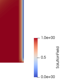
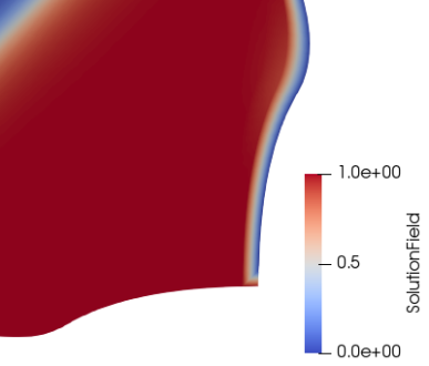
Figure 2: Numerical solutions computed on the unit square (left) and deformed domain (right).

For the diffusion coefficient $d=0.0001$ and the considered basis the element Péclet number is equal to $Pe_{h}\approx 555$, which states that the problem is highly convection-dominated. For the deformed geometry, the actual value varies slightly from one ’element’ to the other but stays in the same order of magnitude.

The numerical solution that was computed on the unit square is depicted in Fig. 2 (left), whereas the approximate solution for the deformed geometry is shown on the right. In both cases the minimum and maximum bounds of the exact solution, that is, $u_{min}=0$ and $u_{max}=1$ are preserved by the numerical counterpart, which results from the successful application of the AFC stabilization of TVD-type.

It should be noted that the internal layer is smeared stronger than the boundary layer, which is due to the constrained $L_{2}$ projection of the Dirichlet boundary data into the space $S^{h}$. The discontinuous profile (8) along the left boundary cannot be represented exactly by quadratic B-Splines, and hence, it is smeared across multiple ’elements’. A possible remedy is to locally reduce the approximation order to $p=1$ by inserting a knot at the boundary location $\eta_{b}=1/5$ and increasing its multiplicity to $m_{b}=2$, which will reduce the continuity to $C^{p-m_{b}}=C^{0}$ locally. The varying thickness of the boundary layer on the deformed geometry stems from the fact the distance of the rightmost vertical internal ’grid line’ to the boundary also varies.

4 Conclusions

The high-resolution isogeometric scheme presented in this work for the stationary convection-diffusion equation is a first step to establish isogeometric methods for convection-dominated problems and, in particular, compressible flows, which are addressed in more detail in igaAFC2_fef2017 . This chapter extends the family of algebraic flux correction schemes to quadratic B-Spline discretizations thereby demonstrating that the algebraic design principles that were originally derived for low-order nodal Lagrange finite elements carry over to non-nodal Spline basis functions.

Ongoing research focuses on the extension of this approach to truncated hierarchical B-Splines Giannelli2012 possibly combined with the local increase of the knot multiplicities, which seems to be a viable approach for refining the spline spaces $S^{h}$ and $V^{h}$ adaptively in the vicinity of shocks and steep gradients to compensate for the local reduction of the approximation order by algebraic flux correction ($h$-refinement) and to prevent excessive spreading of these localized features (continuity reduction).

- [1] M. Möller and A. Jaeschke. High-order isogeometric methods for compressible flows. II. Compressible Euler equations, Accepted for publication, online version available at arXiv.
- [2] T.J.R. Hughes, J.A. Cottrell, and Y. Bazilevs. Isogeometric analysis: CAD, finite elements, NURBS, exact geometry and mesh refinement. Computer Methods in Applied Mechanics and Engineering, 194(39–41):4135 – 4195, 2005.
- [3] J.A. Cottrell, T.J.R. Hughes, and Y. Bazilevs. Isogeometric Analysis: Toward Integration of CAD and FEA. John Wiley & Sons, Ltd., 2009.
- [4] P. Trontin. Isogeometric analysis of Euler compressible flow. Application to aerodynamics. 50th AIAA, 2012.
- [5] A. Jaeschke. Isogeometric analysis for compressible flows with application in turbomachinery. Master’s thesis, Delft University of Technology, 2015.
- [6] A.N. Brooks and T.J.R. Hughes. Streamline upwind/Petrov-Galerkin formulations for convection dominated flows with particular emphasis on the incompressible Navier-Stokes equations. Computer Methods in Applied Mechanics and Engineering, 32(1–3):199 – 259, 1982.
- [7] D. Kuzmin and S. Turek. Flux correction tools for finite elements. Journal of Computational Physics, 175(2):525 – 558, 2002.
- [8] D. Kuzmin and S. Turek. High-resolution FEM-TVD schemes based on a fully multidimensional flux limiter. Journal of Computational Physics, 198(1):131 – 158, 2004.
- [9] D. Kuzmin and M. Möller. Flux-Corrected Transport, chapter Algebraic flux correction I. Scalar conservation laws. Springer, 2005.
- [10] D. Kuzmin. On the design of general-purpose flux limiters for finite element schemes. I. Scalar convection. Journal of Computational Physics, 219(2):513 – 531, 2006.
- [11] D. Kuzmin. Algebraic flux correction for finite element discretizations of coupled systems. Computational Methods for Coupled Problems in Science and Engineering II, CIMNE, Barcelona, pages 653–656, 2007.
- [12] D. Kuzmin, M. Möller, J.N. Shadid, and M. Shashkov. Failsafe flux limiting and constrained data projections for equations of gas dynamics. Journal of Computational physics, 229(23):8766–8779, 11 2010.
- [13] D. Kuzmin. Flux-Corrected Transport, chapter Algebraic flux correction I. Scalar conservation laws. Springer, 2012.
- [14] D. Kuzmin, M. Möller, and M. Gurris. Flux-Corrected Transport, chapter Algebraic flux correction II. Compressible flow problems. Springer, 2012.
- [15] C. de Boor. Subroutine package for calculating with B-splines. Technical Report LA-4728-MS, Los Alamos Scient. Lab., 1971.
- [16] C.A.J. Fletcher. The group finite element formulation. Comput. Methods Appl. Mech. Eng, 37:225–243, 1983.
- [17] I. Farago, R. Horvath, and S. Korotov. Discrete maximum principle for linear parabolic problems solved on hybrid meshes. Applied Numerical Mathematics, 53(2-4):249–264, 05 2004.
- [18] D. Kuzmin, M.J. Shashkov, and D. Svyatski. A constrained finite element method satisfying the discrete maximum principle for anisotropic diffusion problems on arbitrary meshes, 2008.
- [19] S.K. Godunov. Finite difference method for numerical computation of discontinous solutions of the equations of fluid dynamics. Mat. Sbornik, 47:271–306, 1959.
- [20] H.F. Walker and P. Ni. Anderson acceleration for fixed-point iterations. SIAM J. Numer. Anal., 49(4):1715–1735, 08 2011.
- [21] M. Möller. Efficient solution techniques for implicit finite element schemes with flux limiters. International Journal for Numerical Methods in Fluids, 55(7):611–635, 11 2007.
- [22] B. Jüttler, U. Langer, A. Mantzaflaris, S. Moore, and W. Zulehner. Geometry + Simulation Modules: Implementing isogeometric analysis. Proc. Appl. Math. Mech., 14(1):961–962, 2014. Special Issue: 85th Annual Meeting of the Int. Assoc. of Appl. Math. and Mech. (GAMM), Erlangen 2014.
- [23] C. Giannelli, B. Jüttler, and H. Speleers. THB-splines: The truncated basis for hierarchical splines. Computer Aided Geometry Design, 29(7):485–498, 10 2012.