Tutorial: Concepts and numerical techniques for modeling individual phonon transmission at interfaces

Abstract

At the nanoscale, thermal transport across the interface between two lattice insulators can be described by the transmission of bulk phonons and depends on the crystallographic structure of the interface and the bulk crystal lattice. In this tutorial, we give an account of how an extension of the Atomistic Green’s Function (AGF) method based on the concept of the Bloch matrix can be used to model the transmission of individual phonon modes and allow us to determine the wavelength and polarization dependence of the phonon transmission. Within this framework, we can explicitly establish the relationship between the phonon transmission coefficient and dispersion. Details of the numerical methods used in the extended AGF method are provided. To illustrate how the extended AGF method can be applied to yield insights into individual phonon transmission, we study the (16,0)/(8,0) carbon nanotube intramolecular junction. The method presented here sheds light on the modal contribution to interfacial thermal transport between solids.

I Introduction

Heat conduction between dissimilar non-metallic materials is at present a topic of increasing relevance for technological development in nanoelectronics, optoelectronics, nanomechanics and thermoelectrics because of the heat dissipation issues associated with high temperatures and power densities which limit device performance. One of the basic challenges to efficient heat dissipation in semiconductors and insulators at the nanoscale is the thermal boundary resistance which arises from incomplete phonon transmission across the crystallographic interface. (Pop, 2010) On the other hand, the impedance of thermal transport by interfaces may be exploited for thermoelectric applications (Cahill et al., 2003; Pop, 2010; Cahill et al., 2014; Chen et al., 2013). Therefore, a substantial amount of experimental and theoretical work (Cahill et al., 2003, 2014) has been motivated by the desire to advance our understanding of interfacial phonon transmission and its role in interfacial thermal transport.

In most theories of phonon-mediated interfacial thermal transport, (Chen, 2005) it is assumed that energy is dissipated across an interface when an incident bulk phonon, propagating in one medium towards the other, crosses the interface with the probability of transmission given by the phonon transmission coefficient. This physical picture underlies the two major acoustics-based analogies, (Swartz and Pohl, 1989; Chen, 2005) the acoustic mismatch model (AMM) and the diffuse mismatch model (DMM), commonly used to interpret experimental (Costescu et al., 2003) and simulation-based studies (Schelling et al., 2002) of interfacial thermal transport. However, in spite of their widespread use in modeling thermal boundary resistance, they suffer from several shortcomings. Firstly, they typically adopt an idealized model of the phonon dispersion and ignore the contribution from optical phonon modes. Secondly, they cannot determine the dependence of phonon transmission on the atomistic structure of the interface as phonon scattering by the interface is assumed to be either completely specular (in the AMM) or diffusive (in the DMM).

On the other hand, the relationship between the atomistic structure of the interface and phonon transmission can be studied using the Atomistic Green’s Function (AGF) method developed by Mingo and Yang, (Mingo and Yang, 2003) a highly versatile lattice dynamics-based technique which can be coupled to either empirical (Zhang et al., 2007a, b) or ab initio-based models of interatomic forces (Tian et al., 2012) and has proved to be a powerful tool for studying ballistic phonon transport in atomistic models; (Zhang et al., 2007b) the technique has been applied to graphene grain boundaries (Lu and Guo, 2012; Serov et al., 2013), silicon-germanium heterostructures (Zhang et al., 2007a; Huang et al., 2011; Tian et al., 2012) and superlattices. (Luckyanova et al., 2012) In addition, significant recent progress has been made in the development of molecular dynamics simulation techniques for determining the frequency-dependent spectral content of the thermal boundary conductance. (Sääskilahti et al., 2014; Zhou and Hu, 2017) However, one of the principal drawbacks of the traditional AGF method (Zhang et al., 2007b, a; Huang et al., 2011) is its inability to describe individual phonon transmission explicitly in terms of the bulk phonon dispersion, unlike the AMM where the individual phonon transmission coefficients can be determined, potentially limiting our understanding of the physical processes in nanoscale interfacial thermal transport and their dependence on atomistic structure.

However, a straightforward and efficient extension of the existing AGF methodology has been developed recently developed in Ref. (Ong and Zhang, 2015) to describe the ballistic transmission of individual phonon modes and their dependence on polarization, frequency ($\omega$), and wave vector ($\mathbf{k}$), connecting the transmission coefficient to phonon dispersion. A key ingredient of this extension of the AGF method is the notion of the Bloch matrix which can be derived from the surface Green’s function and yields the bulk phonon modes that constitute the individual transmission channels. Conceptually, this extension of the AGF method bridges the gap between the existing AGF method, in which the connection between transmittance and phonon dispersion is obscure, and the analytical theories of the AMM and DMM, where the individual phonon transmission coefficients can be computed but the dependence on the atomistic structure of the interface is unclear.

In this tutorial, we will not review the general phenomenon of nanoscale interfacial thermal transport, as several excellent review articles have been written, (Swartz and Pohl, 1989; Cahill et al., 2003, 2014) but rather, describe the technique of the aforementioned extension of the Atomistic Green’s Function (AGF) method, (Ong and Zhang, 2015) which we will call the extended AGF method in the rest of the paper, for calculating the ballistic transmission of individual phonons. It is hoped that after reading this tutorial article, the reader will gain a better understanding of the practical steps involved in calculating individual phonon transmission coefficients. The organization of the rest of the tutorial is as follows. We first review and describe the traditional AGF method in terms of the numerical inputs and how the calculations are set up. Next, we describe how the Bloch matrices are derived from the surface Green’s functions used in the traditional AGF method, and show how the Bloch matrices can be exploited to determine the phonon eigenmode and velocity matrices which can be combined with the Green’s function of the scattering region to yield the transmission matrices and individual phonon transmission coefficients. We demonstrate the basic ideas of the extended AGF method using the simple first example of a linear atomic chain junction. To illustrate the application of the extended AGF method to more realistic systems, we simulate phonon transmission across the (16,0)/(8,0) carbon nanotube intramolecular junction (Wu and Li, 2007) and analyze how the phonon transmission coefficients depend on polarization, frequency and wavelength.

I.1 Review of traditional AGF method

The AGF method is derived from the well-known nonequilibrium Green’s function (NEGF) method used in the modeling of tight-binding electron transport (Klimeck et al., 1995; Nardelli, 1999) and many excellent pedagogical resources on the NEGF method have been made available by S. Datta. (Datta, 1997, 2000; SDa, ) The key idea in the NEGF method (Datta, 1997) is that in the Landauer-Büttiker picture, (Landauer, 1989) the electrical current in the channel arises from the transmission of electrons between the leads and is determined from the energy-dependent transmission function or transmittance computed from the Green’s function of the system. In actual numerical implementation, the Green’s function is evaluated from a tight-binding Hamiltonian model. (Datta, 2000)

The application of the NEGF method to thermal transport in realistic atomistic structures was first formulated by Mingo and Yang who used the AGF method to describe phonon flow in an atomistic model of silica-coated silicon nanowires. (Mingo and Yang, 2003) A more detailed and highly readable account of the AGF approach is given in Ref. (Mingo, 2009). Like in the electron NEGF method, the phonon current in the lattice is determined by a frequency-dependent transmittance which depends on the Green’s function derived from the force-constant matrix $\mathbf{K}$ describing the vibrational character of the lattice, instead of the tight-binding Hamiltonian. The nondiagonal elements of $\mathbf{K}$ are given by, for $i\neq j$,

$$K_{ij}=\frac{\partial^{2}E}{\partial u_{i}\partial u_{j}}\ ,$$ (1)

where $E$ is the total lattice energy and $u_{i}$ is the displacement of the $i$-th atomic degree of freedom with respect to its equilibrium value. The expression in Eq. (1) is just the Hessian matrix and is symmetric. The acoustic sum rule implies that the diagonal elements of $\mathbf{K}$ can be obtained from the condition $K_{ii}=-\sum_{j}K_{ij}$.

If we take $\omega$ to be the vibrational frequency, then the equation of motion in frequency space for the system is

$$(\omega^{2}\mathbf{M}-\mathbf{K})\mathbf{u}=\mathbf{0}$$ (2)

where $\mathbf{M}$ is a diagonal matrix with its matrix elements corresponding to the masses of the constituent atoms and $\mathbf{u}$ is a column vector with its elements corresponding to the individual degrees of freedom $u_{i}$. Equation (2) can be rewritten as an eigenvalue equation

$$(\omega^{2}\mathbf{I}-\mathbf{H})\mathbf{\bar{u}}=\bar{\mathbf{0}}$$ (3)

where $\mathbf{H}=\mathbf{M}^{-1/2}\mathbf{K}\mathbf{M}^{-1/2}$ is the mass-normalized harmonic matrix and $\mathbf{\bar{u}}=\mathbf{M}^{1/2}\mathbf{u}$. We can interpret Eq. (3) as the frequency-space equation of motion for the lattice, analogous to the Schrödinger equation which is the equation of motion for the electron wave function, and regard $\mathbf{H}$ as the lattice-dynamical analog of the tight-binding Hamiltonian. Typically, for a system with a finite number of degrees of freedom, the eigenmodes, which are its stationary states, and eigenfrequencies can be found by solving Eq. (3). For an infinite bulk system with translational symmetry, the eigenmodes are called phonons and correspond to the periodic atomic displacements in the lattice. However, the phonon transmittance is not determined by simply solving Eq. (3) which is an eigenvalue equation. The problem of transmission is more complicated conceptually and numerically as it deals with an infinitely large system that lacks the translational symmetry like in a uniform bulk system. Rather, treating phonon transmission involves determining how asymptotic bulk lattice wave excitations, bulk phonons in our case, pass through a localized region and transit to asymptotic bulk lattice wave states on the other side, and this calls on a different method of solution such as the AGF method in which the primary object of study is the transitions between asymptotic bulk phonon states, which are extended infinitely into the bulk, rather than the eigenstates of the lattice.

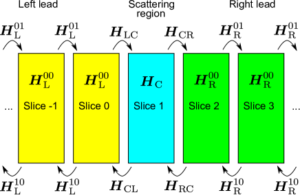
Figure 1: Schematic of scattering system (left lead, scattering region and right lead) and the submatrices associated with each slice or principal layer which represents the set of atomic degrees of freedom for a block row in Eq. (4). The left and right lead each consist of a semi-infinite one-dimensional array of identical slices while the scattering region corresponds to the interface.

I.1.1 Arrangement of system into principal layers

At the interface between two lattices, translational symmetry is broken and the discontinuity in the crystallographic structure results in phonon transmission and reflection by the interface. The AGF method essentially computes the frequency-dependent transmittance for the interface. In the AGF method, the harmonic matrix $\mathbf{H}$ is partitioned into submatrices according to the physical arrangement of the degrees of freedom within our simulation structure. In the partition scheme shown in Fig. 1, there are three subsystems: (1) the left lead, (2) the scattering region and (3) the right lead. The leads correspond to the bulk lattices while the scattering region contains their interface. The leads are each arranged into a semi-infinite one-dimensional array of identical slices (or principal layers) of equal size while the scattering region is considered a slice by itself. The number of degrees of freedom in each slice should be large enough so that only adjacent slices can couple mechanically, and we characterize the spacing between the slices in the lead by the lattice constant $a_{\alpha}$, where $\alpha=\text{L}$ and $\alpha=\text{R}$ for the left and right lead, respectively. Thus, the entire system has an infinite number of slices, each of which can be indexed by an integer that increases as one goes from left to right slice-wise. In our convention, the scattering region is defined as slice $1$ while the principal layers in the left and right lead are enumerated $-\infty,\ldots,0$ and $2,\ldots,+\infty$, respectively.

Given our partitioning scheme, the harmonic matrix $\mathbf{H}$ from Eq. (3) can be structured as a block-tridiagonal matrix,

$$\mathbf{H}=\left(\begin{array}[]{ccccccc}\ddots&\ddots\\ \ddots&\boldsymbol{H}_{\text{L}}^{00}&\boldsymbol{H}_{\text{L}}^{01}\\ &\boldsymbol{H}_{\text{L}}^{10}&\boldsymbol{H}_{\text{L}}^{00}&\boldsymbol{H}_{\text{LC}}\\ &&\boldsymbol{H}_{\text{CL}}&\boldsymbol{H}_{\text{C}}&\boldsymbol{H}_{\text{CR}}\\ &&&\boldsymbol{H}_{\text{RC}}&\boldsymbol{H}_{\text{R}}^{00}&\boldsymbol{H}_{\text{R}}^{01}\\ &&&&\boldsymbol{H}_{\text{R}}^{10}&\boldsymbol{H}_{\text{R}}^{00}&\ddots\\ &&&&&\ddots&\ddots\end{array}\right)$$ (4)

where $\boldsymbol{H}_{\text{C}}$, and $\boldsymbol{H}_{\text{CL}}$ ($\boldsymbol{H}_{\text{CR}}$) are respectively the force-constant submatrices corresponding to the interface region (slice 1) and the coupling between the interface region and the semi-infinite left (right) lead. We can associate each slice in Fig. 1 with a block row and column in $\mathbf{H}$. In the standard AGF setup, the submatrices $\boldsymbol{H}_{\alpha}^{00}$ and $\boldsymbol{H}_{\alpha}^{01}$, where $\alpha=\text{L}$ and $\alpha=\text{R}$ for the left and right lead, respectively, characterize the lead phonons. In the each lead, $\boldsymbol{H}_{\alpha}^{00}$ corresponds to the force-constant submatrix for each slice while $\boldsymbol{H}_{\alpha}^{01}$ ($\boldsymbol{H}_{\alpha}^{10}$) corresponds to the harmonic coupling between each slice and the slice to its right (left) in the lead. In the rest of the paper, we reserve $\alpha$ as the dummy variable for distinguishing the leads, with $\alpha=\text{L}$ and $\alpha=\text{R}$ representing the left and right lead, respectively.

I.1.2 Force-constant matrices and Green’s functions

We note here that in spite of the infinite number of slices making up the system in Fig. 1, only a finite set of unique force-constant matrices ($\boldsymbol{H}_{\text{C}}$, $\boldsymbol{H}_{\text{CL}}$, $\boldsymbol{H}_{\text{CR}}$, $\boldsymbol{H}_{\text{L}}^{00}$, $\boldsymbol{H}_{\text{L}}^{01}$, $\boldsymbol{H}_{\text{R}}^{00}$ and $\boldsymbol{H}_{\text{R}}^{01}$) are needed as inputs for the AGF calculation because the leads are made up of identical slices and the Hermicity of $\mathbf{H}$ implies that $\boldsymbol{H}_{\text{LC}}=(\boldsymbol{H}_{\text{CL}})^{\dagger}$, $\boldsymbol{H}_{\text{RC}}=(\boldsymbol{H}_{\text{CR}})^{\dagger}$, and $\boldsymbol{H}_{\alpha}^{01}=(\boldsymbol{H}_{\alpha}^{10})^{\dagger}$. The periodic arraying of the slices in the leads means that each slice constitutes a unit cell, but not necessarily the primitive unit cell, and that the bulk phonon dispersion, which relates the vibrational frequency $\omega$ to the phonon wave vector $k$, can be determined from the eigenvalue equation

$$[\omega^{2}\boldsymbol{I}_{\alpha}-\boldsymbol{D}_{\alpha}(k)]\boldsymbol{\phi}(k)=\boldsymbol{0}\ ,$$ (5)

where $\boldsymbol{D}_{\alpha}(k)=\boldsymbol{H}_{\alpha}^{10}e^{-ika_{\alpha}}+\boldsymbol{H}_{\alpha}^{00}+\boldsymbol{H}_{\alpha}^{01}e^{ika_{\alpha}}$ is the dynamical matrix and $\boldsymbol{I}_{\alpha}$ is the identity matrix.

In principle, the system dynamics are determined by the infinitely large $\mathbf{H}$ in Eq. (4). However, if we restrict ourselves to describing the oscillatory motion at frequency $\omega$, the problem becomes more tractable as we need only to project the lattice dynamics onto a finite portion of the system, (Wang et al., 2008; Mingo, 2009) corresponding to slices 0 to 2 in Fig. 1, to determine the phonon transmittance through the scattering region (slice 1). Hence, we can use the submatrices in Eq. (4) to construct the effective frequency-dependent harmonic matrix or ‘Hamiltonian’ for this subsystem, as shown in Fig. 2: (Wang et al., 2008)

$$\mathbf{H}^{\prime}=\left(\begin{array}[]{ccc}\boldsymbol{H}_{\text{L}}^{\prime}&\boldsymbol{H}_{\text{LC}}^{\prime}&0\\ \boldsymbol{H}_{\text{CL}}^{\prime}&\boldsymbol{H}_{\text{C}}^{\prime}&\boldsymbol{H}_{\text{CR}}^{\prime}\\ 0&\boldsymbol{H}_{\text{RC}}^{\prime}&\boldsymbol{H}_{\text{R}}^{\prime}\end{array}\right)\ ,$$ (6)

where $\boldsymbol{H}_{\text{L}}^{\prime}=\boldsymbol{H}_{\text{L}}^{00}+\boldsymbol{H}_{\text{L}}^{10}\boldsymbol{g}_{\text{L},-}^{\text{ret}}\boldsymbol{H}_{\text{L}}^{01}$ and $\boldsymbol{H}_{\text{R}}^{\prime}=\boldsymbol{H}_{\text{R}}^{00}+\boldsymbol{H}_{\text{R}}^{01}\boldsymbol{g}_{\text{R},+}^{\text{ret}}\boldsymbol{H}_{\text{R}}^{10}$ represent the left and right edge, respectively while $\boldsymbol{H}_{\text{C}}^{\prime}=\boldsymbol{H}_{\text{C}}$ and $\boldsymbol{H}_{\text{CL/CR}}^{\prime}=\boldsymbol{H}_{\text{CL/CR}}=(\boldsymbol{H}_{\text{LC/RC}}^{\prime})^{\dagger}$. The frequency-dependent retarded surface Green’s functions $\boldsymbol{g}_{\text{L},-}^{\text{ret}}$ and $\boldsymbol{g}_{\text{R},+}^{\text{ret}}$ are given by

$$\boldsymbol{g}_{\alpha,-}^{\text{ret}}=[(\omega^{2}+i\eta)\boldsymbol{I}_{\alpha}-\boldsymbol{H}_{\alpha}^{00}-\boldsymbol{H}_{\alpha}^{10}\boldsymbol{g}_{\alpha,-}^{\text{ret}}\boldsymbol{H}_{\alpha}^{01}]^{-1}$$ (7a)

$$\boldsymbol{g}_{\alpha,+}^{\text{ret}}=[(\omega^{2}+i\eta)\boldsymbol{I}_{\alpha}-\boldsymbol{H}_{\alpha}^{00}-\boldsymbol{H}_{\alpha}^{01}\boldsymbol{g}_{\alpha,+}^{\text{ret}}\boldsymbol{H}_{\alpha}^{10}]^{-1}$$ (7b)

where $\eta$ is the small infinitesimal part that we add to $\omega^{2}$ to satisfy causality, and they are commonly generated using the decimation technique (Guinea et al., 1983) or by solving the generalized eigenvalue equation. (Wang et al., 2008; Sadasivam et al., 2017) Physically, Eq. (7a) is the retarded surface Green’s function for a decoupled semi-infinite lattice extending infinitely to the left (denoted by the ‘-’ in the subscript of $\boldsymbol{g}_{\alpha,-}^{\text{ret}}$) while Eq. (7b) is the corresponding surface Green’s function for a decoupled semi-infinite lattice extending infinitely to the right (denoted by the ‘+’ in the subscript of $\boldsymbol{g}_{\alpha,+}^{\text{ret}}$). In addition, the advanced surface Green’s functions can be obtained from the Hermitian conjugates of Eq. (7b), i.e. $\boldsymbol{g}_{\alpha,-}^{\text{adv}}=(\boldsymbol{g}_{\alpha,-}^{\text{ret}}){}^{\dagger}$ and $\boldsymbol{g}_{\alpha,+}^{\text{adv}}=(\boldsymbol{g}_{\alpha,+}^{\text{ret}})^{\dagger}$.

Figure 2: Schematic of the finite projected system in Eq. (6), consisting of the scattering region (slice $1$) and its terminated edges (slices $0$ and $2$). The frequency-dependent dynamics of the semi-infinite leads are implicitly included in $\boldsymbol{H}_{\text{L}}^{\prime}$ and $\boldsymbol{H}_{\text{R}}^{\prime}$ through the surface Green’s functions $\boldsymbol{g}_{\text{L},-}^{\text{ret}}$ and $\boldsymbol{g}_{\text{R},+}^{\text{ret}}$ from which we can derive the incoming and outgoing phonon modes [$\boldsymbol{U}_{\text{L}}^{\text{adv/ret}}(-)$ and $\boldsymbol{U}_{\text{R}}^{\text{adv/ret}}(+)$] and their group velocities [$\boldsymbol{V}_{\text{L}}^{\text{adv/ret}}(-)$ and $\boldsymbol{V}_{\text{R}}^{\text{adv/ret}}(+)$].

I.1.3 Phonon transmittance and current

To find the phonon transmission through the interface, we compute the corresponding Green’s function for Eq. (6), $\boldsymbol{G}^{\text{ret}}=[(\omega^{2}+i\eta)\mathbf{I}^{\prime}-\mathbf{H}^{\prime}]^{-1}$ where $\mathbf{I}^{\prime}$ is an identity matrix of the same size as $\mathbf{H}^{\prime}$; the $\boldsymbol{G}^{\text{ret}}$ matrix can be partitioned into submatrices in the same manner as $\mathbf{H}^{\prime}$, i.e.

$$\boldsymbol{G}^{\text{ret}}=\left(\begin{array}[]{ccc}\boldsymbol{G}_{\text{L}}^{\text{ret}}&\boldsymbol{G}_{\text{LC}}^{\text{ret}}&\boldsymbol{G}_{\text{LR}}^{\text{ret}}\\ \boldsymbol{G}_{\text{CL}}^{\text{ret}}&\boldsymbol{G}_{\text{C}}^{\text{ret}}&\boldsymbol{G}_{\text{CR}}^{\text{ret}}\\ \boldsymbol{G}_{\text{RL}}^{\text{ret}}&\boldsymbol{G}_{\text{RC}}^{\text{ret}}&\boldsymbol{G}_{\text{R}}^{\text{ret}}\end{array}\right)\ .$$ (8)

In the original AGF method,(Zhang et al., 2007b; Wang et al., 2008) the phonon transmittance through the scattering region is given by the well-known Caroli formula: (Caroli et al., 1971; Zhang et al., 2007b; Wang et al., 2008)

$$\Xi(\omega)=\text{Tr}[\boldsymbol{\Gamma}_{\text{R}}\boldsymbol{G}_{\text{RL}}^{\text{ret}}\boldsymbol{\Gamma}_{\text{L}}(\boldsymbol{G}_{\text{RL}}^{\text{ret}})^{\dagger}]$$ (9)

where $\boldsymbol{\Gamma}_{\text{L}}=i\boldsymbol{H}_{\text{L}}^{10}(\boldsymbol{g}_{\text{L},-}^{\text{ret}}-\boldsymbol{g}_{\text{L},-}^{\text{adv}})\boldsymbol{H}_{\text{L}}^{01}$ and $\boldsymbol{\Gamma}_{\text{R}}=i\boldsymbol{H}_{\text{R}}^{01}(\boldsymbol{g}_{\text{R},+}^{\text{ret}}-\boldsymbol{g}_{\text{R},+}^{\text{adv}})\boldsymbol{H}_{\text{R}}^{10}$, while the total phonon heat flux between the leads is given by

$$J(\omega)=\int_{0}^{\infty}d\omega\frac{\hbar\omega}{2\pi}[f_{\text{L}}(\omega)-f_{\text{R}}(\omega)]\Xi(\omega)$$ (10)

where $f_{\alpha}(\omega)=[\exp(\frac{\hbar\omega}{k_{B}T_{\alpha}})-1]^{-1}$ is the Bose-Einstein occupation factor for the $\alpha$ lead at temperature $T_{\alpha}$.

I.2 Recent extensions of AGF method for mode-resolved transmission

At this point, we depart from the usual AGF method to describe how the traditional AGF formalism can be extended to find the constituent phonons in the heat flux in Eq. (10). From the Green’s function $\boldsymbol{G}^{\text{ret}}$ in Eq. (8), we can use the traditional AGF method to compute the phonon transmittance $\Xi(\omega)$ which is the sum of the individual phonon transmission coefficients. (Huang et al., 2011; Ong and Zhang, 2015) A more explicit connection to conventional scattering theory may be made by noting that the individual transmission coefficients can be derived directly from the diagonal elements of the transmission matrix, (Fisher and Lee, 1981) which relates the amplitude of the incoming phonon flux to that of the outgoing forward-scattered (or transmitted) phonon flux and is computed numerically from $\boldsymbol{G}^{\text{ret}}$. (Ong and Zhang, 2015)

I.2.1 Bloch matrices and bulk phonon eigenmodes

As a prerequisite to computing the transmission coefficient of individual phonon modes at a given $\omega$, we need to determine all the individual phonon modes which can be derived from surface Green’s functions in Eq. (7b). We motivate the following derivation by first pointing out that the surface Green’s functions for the $\alpha$ lead depend only on $\boldsymbol{H}_{\alpha}^{00}$ and $\boldsymbol{H}_{\alpha}^{01}$, which are also the matrices used to find the bulk phonon eigenmodes in Eq. (5), suggesting that properties of the bulk phonons are encoded in the surface Green’s function matrices.

The link between the surface Green’s function and the bulk phonon eigenmodes may be more firmly established by noting that the advanced and retarded Bloch matrices (Ando, 1991; Khomyakov et al., 2005; Ong and Zhang, 2015) of the left and right lead, $\boldsymbol{F}_{\alpha}^{\text{adv/ret}}(+)$ and $\boldsymbol{F}_{\alpha}^{\text{adv/ret}}(-)$, which describe the bulk translational symmetry along the direction of the heat flux, can be computed directly from the formulae:

$$\boldsymbol{F}_{\alpha}^{\text{adv/ret}}(+)=\boldsymbol{g}_{\alpha,+}^{\text{adv/ret}}\boldsymbol{H}_{\alpha}^{10}$$ (11a)

$$\boldsymbol{F}_{\alpha}^{\text{adv/ret}}(-)^{-1}=\boldsymbol{g}_{\alpha,-}^{\text{adv/ret}}\boldsymbol{H}_{\alpha}^{01}\ .$$ (11b)

As pointed out in Ref. (Ong and Zhang, 2015), the bulk eigenmodes for the lead at frequency $\omega$ can be determined directly from the Bloch matrices by solving the eigenvalue equations:

$$\boldsymbol{F}_{\alpha}^{\text{adv/ret}}(+)\boldsymbol{U}_{\alpha}^{\text{adv/ret}}(+)=\boldsymbol{U}_{\alpha}^{\text{adv/ret}}(+)\boldsymbol{\Lambda}_{\alpha}^{\text{adv/ret}}(+)$$ (12a)

$$\boldsymbol{F}_{\alpha}^{\text{adv/ret}}(-)^{-1}\boldsymbol{U}_{\alpha}^{\text{adv/ret}}(-)=\boldsymbol{U}_{\alpha}^{\text{adv/ret}}(-)\boldsymbol{\Lambda}_{\alpha}^{\text{adv/ret}}(-)^{-1}$$ (12b)

where $\boldsymbol{U}_{\alpha}^{\text{ret}}(+)$ [$\boldsymbol{U}_{\alpha}^{\text{ret}}(-)$] is a matrix with its column vectors corresponding to the retarded rightward-going (leftward-going) extended or rightward (leftward) decaying evanescent modes at frequency $\omega$ and has the form $\boldsymbol{U}_{\alpha}^{\text{ret}}=(\boldsymbol{e}_{1}\boldsymbol{e}_{2}\ldots\boldsymbol{e}_{N})$ where $\boldsymbol{e}_{n}$ is a normalized right eigenvector of the Bloch matrix in the $n$-th column of $\boldsymbol{U}_{\alpha}^{\text{ret}}$. Similarly, $\boldsymbol{U}_{\alpha}^{\text{adv}}(-)$ [$\boldsymbol{U}_{\alpha}^{\text{adv}}(+)$] is a matrix with its column vectors corresponding to the advanced rightward-going (leftward-going) extended or leftward (rightward) decaying evanescent modes. The matrix $\boldsymbol{\Lambda}_{\alpha}^{\text{adv/ret}}(+)$ [$\boldsymbol{\Lambda}_{\alpha}^{\text{adv/ret}}(-)$] is a diagonal matrix with matrix elements of the form $e^{ik_{n}a}$ where $k_{n}$ is the phonon wave vector corresponding to the $n$-th column eigenvector in $\boldsymbol{U}_{\alpha}^{\text{adv/ret}}(+)$ [$\boldsymbol{U}_{\alpha}^{\text{adv/ret}}(-)$] and satisfying $-\frac{\pi}{a_{\alpha}}<k_{n}\leq\frac{\pi}{a_{\alpha}}$. At this juncture, it would appear that we have two redundant sets of eigenmodes, $\boldsymbol{U}_{\alpha}^{\text{ret}}(\pm)$ and $\boldsymbol{U}_{\alpha}^{\text{adv}}(\pm)$, although it can be shown later that the former (retarded modes) corresponds to outgoing transmitted phonons while the latter (advanced modes) corresponds to phonons that are incident on the interface.

We note that because the Bloch matrices are not Hermitian, their eigenvectors are not necessarily orthogonal and this can be problematic for transmission coefficient calculations (Sadasivam et al., 2017) when the eigenvectors have the same $k$ and are wave vector-degenerate, i.e. they have the same $\omega$ and $k$. We resolve this by orthonormalizing the wave vector-degenerate column eigenvectors in $\boldsymbol{U}_{\alpha}^{\text{adv/ret}}$ with a Gram-Schmidt procedure. (Arfken and Webber, 1995; Werneth et al., 2010) The final piece of ingredient needed for the calculation of the individual phonon transmission coefficients is the diagonal eigenvelocity matrix (Khomyakov et al., 2005; Wang et al., 2008)

$$\boldsymbol{V}_{\alpha}^{\text{adv/ret}}(+)=\frac{ia_{\alpha}}{2\omega}[\boldsymbol{U}_{\alpha}^{\text{adv/ret}}(+)]^{\dagger}\boldsymbol{H}_{\alpha}^{01}[\boldsymbol{g}_{\alpha,+}^{\text{adv/ret}}-(\boldsymbol{g}_{\alpha,+}^{\text{ret/adv}})^{\dagger}]\boldsymbol{H}_{\alpha}^{10}\boldsymbol{U}_{\alpha}^{\text{adv/ret}}(+)\ ,$$ (13)

which has the group velocities of the eigenvectors in $\boldsymbol{U}_{\alpha}^{\text{adv/ret}}(+)$ as its diagonal elements. Likewise, $\boldsymbol{V}_{\alpha}^{\text{adv/ret}}(-)$ is defined as

$$\boldsymbol{V}_{\alpha}^{\text{adv/ret}}(-)=-\frac{ia_{\alpha}}{2\omega}[\boldsymbol{U}_{\alpha}^{\text{adv/ret}}(-)]^{\dagger}\boldsymbol{H}_{\alpha}^{10}[\boldsymbol{g}_{\alpha,-}^{\text{adv/ret}}-(\boldsymbol{g}_{\alpha,-}^{\text{ret/adv}})^{\dagger}]\boldsymbol{H}_{\alpha}^{01}\boldsymbol{U}_{\alpha}^{\text{adv/ret}}(-)\ .$$ (14)

For the evanescent modes, the group velocity is always zero while for propagating modes that contribute to the heat flux, the group velocity is positive (negative) in $\boldsymbol{V}_{\alpha}^{\text{ret}}(+)$ and $\boldsymbol{V}_{\alpha}^{\text{adv}}(-)$ [$\boldsymbol{V}_{\alpha}^{\text{ret}}(-)$ and $\boldsymbol{V}_{\alpha}^{\text{adv}}(+)$]. In addition, we define the diagonal matrices $\widetilde{\boldsymbol{V}}_{\alpha}^{\text{adv/ret}}(+)$ and $\widetilde{\boldsymbol{V}}_{\alpha}^{\text{adv/ret}}(-)$ in which their nonzero diagonal matrix elements are the inverse of those of $\boldsymbol{V}_{\alpha}^{\text{adv/ret}}(+)$ and $\boldsymbol{V}_{\alpha}^{\text{adv/ret}}(-),$ respectively. For each lead, we can also define the diagonal matrices

$$\boldsymbol{I}_{\alpha}^{\text{adv/ret}}(+)=\boldsymbol{V}_{\alpha}^{\text{adv/ret}}(+)\widetilde{\boldsymbol{V}}_{\alpha}^{\text{adv/ret}}(+)$$ (15a)

$$\boldsymbol{I}_{\alpha}^{\text{adv/ret}}(-)=\boldsymbol{V}_{\alpha}^{\text{adv/ret}}(-)\widetilde{\boldsymbol{V}}_{\alpha}^{\text{adv/ret}}(-)$$ (15b)

in which the $n$-th diagonal element equals $1$ if the $n$-th column of $\boldsymbol{U}_{\alpha}^{\text{adv/ret}}(+)$ and $\boldsymbol{U}_{\alpha}^{\text{adv/ret}}(-)$ corresponds to an extended mode and $0$ otherwise. Therefore, it follows from Eq. (15b ) that the number of rightward-going phonon channels $N_{\alpha}(+)$ and the number of leftward-going phonon channels $N_{\alpha}(-)$ are given by

$$N_{\alpha}(+)=\text{Tr}[\boldsymbol{I}_{\alpha}^{\text{ret}}(+)]=\text{Tr}[\boldsymbol{I}_{\alpha}^{\text{adv}}(-)]$$ (16a)

$$N_{\alpha}(-)=\text{Tr}[\boldsymbol{I}_{\alpha}^{\text{ret}}(-)]=\text{Tr}[\boldsymbol{I}_{\alpha}^{\text{adv}}(+)]\ .$$ (16b)

I.2.2 Phonon transmission matrices and transmission coefficients

Now, let us consider the scattering problem for an incoming phonon at frequency $\omega$ from the left lead that is incident on the scattering region. In the $n=0$ slice at the edge of the left lead, the motion of the degrees of freedom, $\boldsymbol{c}_{0}=(c_{0,1},\ldots,c_{0,N})^{T}$ where $c_{0,l}$ is the complex coefficient for the $l$th degree of freedom in the slice for $l=1,\ldots,N$, can be decomposed into two parts, i.e.

$$\boldsymbol{c}_{0}=\boldsymbol{c}_{0}(+)+\boldsymbol{c}_{0}(-)$$ (17)

where $\boldsymbol{c}_{0}(+)$ and $\boldsymbol{c}_{0}(-)$ respectively represent the rightward-going (incident) and leftward-going (reflected) components, while in the $n=2$ slice at the edge of the right lead, the motion of its degrees of freedom is given by

$$\boldsymbol{c}_{2}=\boldsymbol{c}_{2}(+)\ ,$$ (18)

where the RHS represents a rightward-going (transmitted) $\omega$-frequency wave which can be a linear combination of bulk right-lead phonon modes propagating away from the interface. Suppose the rightward-going component in Eq. (17) is a left-lead bulk phonon mode, i.e. $\boldsymbol{c}_{0}(+)=\boldsymbol{u}_{\text{L},n}(k,\omega)$ where $n$ and $k$ are the phonon polarization index and wave vector, respectively. Then, it can be shown (Khomyakov et al., 2005) that the transmitted wave $\boldsymbol{c}_{2}(+)$ in the right lead is related to the incident wave $\boldsymbol{c}_{0}(+)$ from the right lead, via the expression

$$\boldsymbol{c}_{2}=\boldsymbol{G}_{\text{RL}}^{\text{ret}}\boldsymbol{Q}_{\text{L}}\boldsymbol{u}_{\text{L},n}(k,\omega)$$ (19)

where

$$\boldsymbol{Q}_{\alpha}=(\omega^{2}+i\eta)\boldsymbol{I}_{\alpha}-\boldsymbol{H}_{\alpha}^{00}-\boldsymbol{H}_{\alpha}^{10}\boldsymbol{g}_{\alpha,-}^{\text{ret}}(\omega)\boldsymbol{H}_{\alpha}^{01}-\boldsymbol{H}_{\alpha}^{01}\boldsymbol{g}_{\alpha,+}^{\text{ret}}(\omega)\boldsymbol{H}_{\alpha}^{10}$$ (20)

and $\boldsymbol{Q}_{\alpha}^{-1}$ is the bulk Green’s function of the $\alpha$ lead. The expression in Eq. (19) can be expressed as a linear combination of transmitted right-lead phonon modes $\boldsymbol{u}_{\text{R},m}(k_{m},\omega)$, i.e. $\boldsymbol{c}_{2}=\sum_{m}\boldsymbol{u}_{\text{R},m}(k_{m},\omega)\tau_{mn}$, where $\tau_{mn}$ is the linear coefficient and forms the matrix elements of the transmission matrix $\boldsymbol{\tau}$, where

$$\boldsymbol{\tau}=[\boldsymbol{U}_{\text{R}}^{\text{ret}}(+)]^{-1}\boldsymbol{G}_{\text{RL}}^{\text{ret}}\boldsymbol{Q}_{\text{L}}\boldsymbol{U}_{\text{L}}^{\text{ret}}(+)\ .$$ (21)

The flux-normalized transmission matrix is $\boldsymbol{t}_{\text{RL}}=[\boldsymbol{V}_{\text{R}}^{\text{ret}}(+)]^{\nicefrac{{1}}{{2}}}\boldsymbol{\tau}[\widetilde{\boldsymbol{V}}_{\text{L}}^{\text{adv}}(-)]^{\nicefrac{{1}}{{2}}}$, which we can rewrite as (Ong and Zhang, 2015)

$$\boldsymbol{t}_{\text{RL}}=\frac{2i\omega}{\sqrt{a_{\text{R}}a_{\text{L}}}}[\boldsymbol{V}_{\text{R}}^{\text{ret}}(+)]^{\nicefrac{{1}}{{2}}}[\boldsymbol{U}_{\text{R}}^{\text{ret}}(+)]^{-1}\boldsymbol{G}_{\text{RL}}^{\text{ret}}[\boldsymbol{U}_{\text{L}}^{\text{adv}}(-)^{\dagger}]^{-1}[\boldsymbol{V}_{\text{L}}^{\text{adv}}(-)]^{\nicefrac{{1}}{{2}}}\ .$$ (22)

Each row of $\boldsymbol{t}_{\text{RL}}$ corresponds to either a transmitted right-lead extended or evanescent mode. For an outgoing evanescent mode, the row elements and group velocity, given by the corresponding diagonal element of $\boldsymbol{V}_{\text{R}}^{\text{ret}}(+)$, are zero. Conversely, each column of of $\boldsymbol{t}_{\text{RL}}$ corresponds to either an incident left-lead extended or evanescent mode, and the column elements and group velocity of the evanescent modes, given by the diagonal element of $\boldsymbol{V}_{\text{L}}^{\text{adv}}(-)$. If the $m$-th row and $n$-th column of $\boldsymbol{t}_{\text{RL}}$ correspond to extended transmitted and incident modes, then $|[\boldsymbol{t}_{\text{RL}}]_{mn}|^{2}$ gives us the probability that the incident left-lead phonon is transmitted across the interface into the right-lead phonon. Similarly, we can define the flux-normalized transmission matrix for phonon transmission from the right to the left lead:

$$\boldsymbol{t}_{\text{LR}}=\frac{2i\omega}{\sqrt{a_{\text{L}}a_{\text{R}}}}[\boldsymbol{V}_{\text{L}}^{\text{ret}}(-)]^{\nicefrac{{1}}{{2}}}[\boldsymbol{U}_{\text{L}}^{\text{ret}}(-)]^{-1}\boldsymbol{G}_{\text{LR}}^{\text{ret}}[\boldsymbol{U}_{\text{R}}^{\text{adv}}(+)^{\dagger}]^{-1}[\boldsymbol{V}_{\text{R}}^{\text{adv}}(+)]^{\nicefrac{{1}}{{2}}}\ .$$ (23)

Given Eq. (22), we can construct the smaller rationalized matrices $\bar{\boldsymbol{t}}_{\text{RL}}$ and $\bar{\boldsymbol{t}}_{\text{LR}}$ from $\boldsymbol{t}_{\text{RL}}$ and $\boldsymbol{t}_{\text{LR}}$ by deleting the matrix rows and columns corresponding to evanescent states. This is done numerically by inspecting each diagonal element of $\boldsymbol{I}_{\alpha}^{\text{adv/ret}}(\pm)$ of Eq. (15b), which is either equal to 0 (evanescent) or 1 (extended), and removing the corresponding columns or rows when $[\boldsymbol{I}_{\alpha}^{\text{adv/ret}}(\pm)]_{nn}=0$. For example, to find $\bar{\boldsymbol{t}}_{\text{RL}}$, we inspect $\boldsymbol{I}_{\text{R}}^{\text{ret}}(+)$ for row deletion and $\boldsymbol{I}_{\text{L}}^{\text{adv}}(-)$ for column deletion in $\boldsymbol{t}_{\text{RL}}$. Hence, $\bar{\boldsymbol{t}}_{\text{RL}}$ is a $N_{\text{R}}(+)\times N_{\text{L}}(+)$ matrix. Similarly, we can also define the rationalized smaller matrices $\bar{\boldsymbol{\Lambda}}_{\alpha}^{\text{adv/ret}}(+)$ by deleting the rows and columns associated with evanescent modes from $\boldsymbol{\Lambda}_{\alpha}^{\text{adv/ret}}(\pm)$ in Eq. (12b).

The transmission coefficient of the $n$-th incoming phonon channel in the left lead is defined as the $n$-th diagonal element of $\bar{\boldsymbol{t}}_{\text{RL}}^{\dagger}\bar{\boldsymbol{t}}_{\text{RL}}$, i.e.

$$\Xi_{\text{L},n}=[\bar{\boldsymbol{t}}_{\text{RL}}^{\dagger}\bar{\boldsymbol{t}}_{\text{RL}}]_{nn}\ ,$$ (24)

which is equal to the fraction of its energy flux transmitted across the interface, and its wave vector $k_{n}$ can be determined from $[\bar{\boldsymbol{\Lambda}}_{\text{L}}^{\text{adv}}(-)]_{nn}=e^{ik_{n}a_{\text{L}}}$ or

$$k_{n}=\frac{1}{a_{\text{L}}}\cos^{-1}\text{Re}[\bar{\boldsymbol{\Lambda}}_{\text{L}}^{\text{adv}}(-)]_{nn}\ .$$ (25)

The absorption coefficient of the $l$-th outgoing rightward-going mode in the right lead is given by the $l$-th diagonal element of $\bar{\boldsymbol{t}}_{\text{RL}}\bar{\boldsymbol{t}}_{\text{RL}}^{\dagger}$, i.e.

$$\xi_{\text{R},l}=[\bar{\boldsymbol{t}}_{\text{RL}}\bar{\boldsymbol{t}}_{\text{RL}}^{\dagger}]_{ll}\ ,$$ (26)

with its phonon wave vector $k_{l}$ given by $k_{l}=\frac{1}{a_{\text{R}}}\cos^{-1}\text{Re}[\bar{\boldsymbol{\Lambda}}_{\text{R}}^{\text{ret}}(+)]_{ll}$.

The transmission coefficient for the $n$-th incoming phonon channel in the right lead ($\Xi_{\text{R},n}=[\bar{\boldsymbol{t}}_{\text{LR}}^{\dagger}\bar{\boldsymbol{t}}_{\text{LR}}]_{nn}$) and the absorption coefficient of the $l$-th outgoing phonon channel in the left lead ($\xi_{\text{L},l}=[\bar{\boldsymbol{t}}_{\text{LR}}\bar{\boldsymbol{t}}_{\text{LR}}^{\dagger}]_{ll}$) can be similarly defined like in Eqs. (24) to (26). We remark that the phonon transmittance $\Xi(\omega)$ in Eq. (9) is equal to the sum of the transmission [Eq. (27a)] or absorption [Eq. (27b)] coefficients of either lead, i.e.

$$\Xi(\omega) =\sum_{n=1}^{N_{\text{L}}(+)}\Xi_{\text{L},n}=\sum_{m=1}^{N_{\text{R}}(-)}\Xi_{\text{R},m}\$$ (27a)

$$=\sum_{n=1}^{N_{\text{L}}(-)}\xi_{\text{L},n}=\sum_{m=1}^{N_{\text{R}}(+)}\xi_{\text{R},m}\ ,$$ (27b)

as a consequence of the conservation of probability current.

II Example 1: linear atomic chain

To illustrate the basic ideas of the extended AGF method, we begin with the relatively simple example of the linear atomic chain. We choose this toy model because it has a simple phonon dispersion relation which allows us to ignore the effects of polarization, leading to a more straightforward analysis of the relationship between the phonon transmittance spectrum and the individual phonon transmission coefficients. In the following discussion, sufficient details of our calculations are provided to encourage the reader to reproduce the results shown in Fig. 3.

Figure 3(a) shows the schematic for a linear atomic chain junction, in which the interatomic spacing equals $a$ and the interatomic spring constant between adjacent atoms is $\kappa$; the atomic mass however depends on position. The interface in the center comprises of two atoms with masses $m_{1}$ and $m_{2}$, respectively. For the left lead, we have a semi-infinite atomic chain that has a two-atom unit cell with masses $0.8m$ and $1.2m$, respectively, where $m$ is the characteristic atomic mass scale, and a lattice spacing of $2a$. For the right lead, we have another semi-infinite atomic chain which has a one-atom unit cell with the atomic mass of $m$ and lattice spacing of $a$. Given the model in Fig. 3(a), the harmonic matrices that we use for our AGF calculations are

$$\boldsymbol{H}_{\text{L}}^{00} =\boldsymbol{M}_{\text{L}}^{-1/2}\left(\begin{array}[]{cc}2\kappa&-\kappa\\ -\kappa&2\kappa\end{array}\right)\boldsymbol{M}_{\text{L}}^{-1/2}$$

$$\boldsymbol{H}_{\text{L}}^{01} =\boldsymbol{M}_{\text{L}}^{-1/2}\left(\begin{array}[]{cc}0&0\\ -\kappa&0\end{array}\right)\boldsymbol{M}_{\text{L}}^{-1/2}$$

$$\boldsymbol{H}_{\text{CL}} =\boldsymbol{M}_{\text{C}}^{-1/2}\left(\begin{array}[]{cc}0&-\kappa\\ 0&0\end{array}\right)\boldsymbol{M}_{\text{L}}^{-1/2}$$

$$\boldsymbol{H}_{\text{C}} =\boldsymbol{M}_{\text{C}}^{-1/2}\left(\begin{array}[]{cc}2\kappa&-\kappa\\ -\kappa&2\kappa\end{array}\right)\boldsymbol{M}_{\text{C}}^{-1/2}$$

$$\boldsymbol{H}_{\text{CR}} =\boldsymbol{M}_{\text{C}}^{-1/2}\left(\begin{array}[]{c}0\\ -\kappa\end{array}\right)\boldsymbol{M}_{\text{R}}^{-1/2}$$

$$\boldsymbol{H}_{\text{R}}^{00} =\frac{2\kappa}{m}$$

$$\boldsymbol{H}_{\text{R}}^{01} =-\frac{\kappa}{m}$$

where $\boldsymbol{M}_{\text{L}}=\left(\begin{array}[]{cc}0.8m&0\\ 0&1.2m\end{array}\right)$, $\boldsymbol{M}_{\text{C}}=\left(\begin{array}[]{cc}m_{1}&0\\ 0&m_{2}\end{array}\right)$ and $\boldsymbol{M}_{\text{R}}=m$. In addition, a characteristic frequency scale $\omega_{0}=\sqrt{\kappa/m}$ can be defined.

We use the Caroli formula in Eq. (9) to compute the frequency-dependent transmittance $\Xi(\omega)$ as per the traditional AGF method. For the purpose of demonstrating the extended AGF method, Eqs. (22) to (24) are used to determine the individual phonon transmission coefficients $\Xi_{\text{L},1}$ (left lead) and $\Xi_{\text{R},1}$ (right lead), which we compare to the transmittance calculated with the Caroli formula. Two sets of calculations are performed: one for $m_{1}=2m$ and $m_{2}=m$ and the other for $m_{1}=m$ and $m_{2}=2m$, i.e. we swap the atomic masses in the center.

Figure 3(b) shows the transmittance spectrum obtained for $m_{1}=2m$ and $m_{2}=m$. Generally, $\Xi(\omega)$ decreases with $\omega$ because low-frequency phonons are more easily transmitted through the interface. To understand the contribution of the left-lead phonons to the interfacial heat flux, we superimpose the individual phonon transmission coefficients $\Xi_{\text{L},1}$ on the phonon dispersion curve for the left chain, which has two branches (acoustic and optical) given the two-atom unit cell, in Fig. 3(c). The frequency gap between the bottom of the optical branch and the top of the acoustic branch is due to the difference in the atomic masses of the unit cell and corresponds to the transmittance gap in Fig. 3(b), indicating the lack of available phonon channels for transmission. In Fig. 3(c), only the phonon modes with a positive group velocity ($\partial\omega/\partial k>0$) are shown because they contribute to the left-lead phonon flux incident on the interface. In the acoustic branch, the transmission coefficients $\Xi_{\text{L},1}$ are significantly closer to unity and this explains the higher transmittance in the spectral region below the gap in Fig. 3(b). On the other hand, in the optical branch, the transmission coefficients are closer to zero, corresponding to the diminished transmittance in the spectral region above the gap.

Alternatively, phonon transmission can also be analyzed in terms of the right-lead phonons. In Fig. 3(d), there is only one phonon branch as the linear chain in the right lead has a one-atom unit cell, and only the phonon modes with a negative group velocity ($\partial\omega/\partial k>0$) are shown because they contribute to the right-lead phonon flux incident on the interface. The transmission coefficients $\Xi_{\text{R},1}$ for the right-lead phonons decrease from unity gradually as the frequency increases before dropping abruptly to zero when $\omega/\omega_{0}>1.25$. This sudden drop is due to the absence of phonon channels in the left lead to which the right-lead phonons can be scattered.

Figures 3(e) to (g) show the transmittance and transmission coefficient spectra for a different interfacial configuration where $m_{1}=m$ and $m_{2}=2m$. The change in the values for $m_{1}$ and $m_{2}$ results in a different transmittance spectrum in Fig. 3(e). Nevertheless, because the atomistic structure of the left and right lead are unchanged, the phonon dispersion curves and the $\omega$-$k$ loci of the phonon modes in Figs. 3(f) and (g) are the same as those in Figs. 3(c) and (d). However, transmission coefficient values in Figs. 3(f) and (g) are different because the phonon modes are scattered differently by the center region. Figures 3(e) and (f) show that the marked transmittance improvement in the spectral region above the gap is due to the higher transmission coefficients of the phonon modes near the bottom of the optical branch of the left lead.

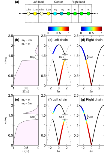
Figure 3: (a) Schematic of junction between two linear atomic chains. (b) Plot of the transmittance $\Xi(\omega)$ as a function of frequency $\omega$ for $m_{1}=2m$ and $m_{2}=m$. The corresponding transmission coefficients for the bulk phonon modes are superimposed on the phonon dispersion curves for the (c) left and (d) right chain. (e) Plot of the transmittance $\Xi(\omega)$ for $m_{1}=m$ and $m_{2}=2m$. The corresponding phonon transmission coefficients for the (f) left and (g) right chain are also shown.

III Example 2: carbon nanotube intramolecular junction

To demonstrate the extended AGF method for a more realistic material system, we use the technique to investigate phonon transmission and thermal transport across the intramolecular junction (IMJ) between a (8,0) and (16,0) carbon nanotube (CNT) as shown in Fig. 4. Like in Ref. (Wu and Li, 2007), two configuration of the (16,0)/(8,0) CNT IMJ are studied, one with 4 heptagon-pentagon defect pairs and the other with 8 heptagon-pentagon defect pairs in the IMJ. We use the example of the CNT IMJ, which has also been studied by Wu and Li, (Wu and Li, 2007) to illustrate the level of detail and type of insights that can be obtained from applying the technique to the simulation of interfacial phonon transmission.

III.1 Generation of interatomic force-constant matrices

The interaction between the C atoms is described by the Tersoff potential, (Tersoff, 1989) with parameters taken from Ref. (Lindsay and Broido, 2010). For each configuration of the (16,0)/(8,0) CNT intramolecular junction, three separate structures – (1) a pristine (16,0) CNT, (2) a pristine (8,0) CNT and (3) the (16,0)/(8,0) CNT IMJ – are optimized using the general utility lattice program (GULP). (Gale and Rohl, 2003) The interatomic force constants needed for the harmonic matrices ($\boldsymbol{H}_{\text{L}}^{00}$, $\boldsymbol{H}_{\text{L}}^{01}$, $\boldsymbol{H}_{\text{CL}}$, $\boldsymbol{H}_{\text{C}}$, $\boldsymbol{H}_{\text{CR}}$, $\boldsymbol{H}_{\text{R}}^{00}$ and $\boldsymbol{H}_{\text{R}}^{01}$) are computed after postprocessing the output from GULP. We extract $\boldsymbol{H}_{\text{L}}^{00}$ and $\boldsymbol{H}_{\text{L}}^{01}$ from the pristine (16,0) CNT, $\boldsymbol{H}_{\text{R}}^{00}$ and $\boldsymbol{H}_{\text{R}}^{01}$ from the pristine (8,0) CNT, and $\boldsymbol{H}_{\text{CL}}$, $\boldsymbol{H}_{\text{C}}$ and $\boldsymbol{H}_{\text{CR}}$ from the (16,0)/(8,0) CNT IMJ for each IMJ configuration.

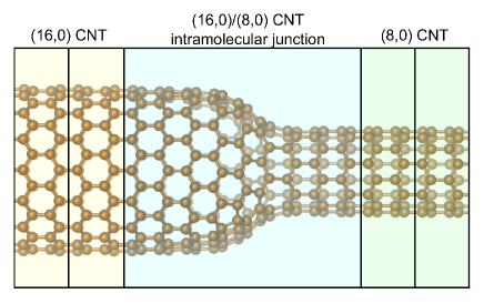
Figure 4: Schematic of the left lead [pristine (16,0) CNT], scattering region [(16,0)/(8,0) CNT IMJ with 4 heptagon-pentagon defect pairs] and right lead [pristine (8,0) CNT] arranged in principal layers or slices as shown in Fig. 1.

III.2 Phonon transmittance and thermal boundary conductance

Given the harmonic matrices ($\boldsymbol{H}_{\text{L}}^{00}$, $\boldsymbol{H}_{\text{L}}^{01}$, $\boldsymbol{H}_{\text{CL}}$, $\boldsymbol{H}_{\text{C}}$, $\boldsymbol{H}_{\text{CR}}$, $\boldsymbol{H}_{\text{R}}^{00}$ and $\boldsymbol{H}_{\text{R}}^{01}$), we use Eq. (9) to compute the phonon transmittance $\Xi(\omega)$ of the (16,0)/(8,0) CNT IMJ for 4 and 8 heptagon-pentagon defect pairs. Likewise, the total phonon transmittance for the pristine (16,0) CNT [$N_{\text{L}}(+)$] and pristine (8,0) CNT [$N_{\text{R}}(-)$] are computed from Eq. (16b). Figure 5(a) shows $\Xi(\omega)$ for 4 and 8 defect pairs as well as the transmittance $N_{\text{L}}(+)$ and $N_{\text{R}}(-)$ through the pristine (16,0) and (18,0) CNT, respectively. In the rest of the discussion, we denote the phonon transmittance for the CNT IMJ with $n$ defect pairs as $\Xi_{n\text{-hp}}(\omega)$. Given that the (16,0) CNT has a larger cross section than the (8,0) CNT, we have $N_{\text{L}}(+)>N_{\text{R}}(-)$ for all frequencies and thus, the phonon transmittance $\Xi_{n\text{-hp}}(\omega)$ through the CNT IMJ is bounded by $N_{\text{R}}(-)$ as expected. The spectrum in Fig. 5(a) also shows that $\Xi_{8\text{-hp}}(\omega)<\Xi_{4\text{-hp}}(\omega)$ for almost all $\omega$ values, consistent with Wu and Li’s finding (Wu and Li, 2007) that the CNT IMJ with 8 defects pairs has a higher thermal resistance than the CNT IMJ with 4 defects pairs. Figure 5(b) also shows the normalized phonon density of states for the pristine (16,0) and (8,0) CNTs which are very similar.

The thermal boundary conductance of the CNT IMJ with $n$ heptagon-pentagon defect pairs can be determined using the Landauer formalism (Landauer, 1989) and is given by

$$G_{\text{IMJ}}^{n\text{-hp}}(T)=\frac{1}{2\pi}\int d\omega\ \hbar\omega\frac{df(\omega,T)}{dT}\Xi_{n\text{-hp}}(\omega)\ ,$$ (28)

where $f(\omega,T)$ is the usual Bose-Einstein distribution function $f(\omega,T)=[\exp(\frac{\hbar\omega}{k_{B}T})-1]^{-1}$ at temperature $T$. We also use Eq. (28) to compute the temperature-dependence thermal conductance for pristine (16,0) CNT ($G_{\text{(16,0)}}$) and pristine (8,0) CNT ($G_{\text{(8,0)}}$) by using $N_{\text{L}}(+)$ [$N_{\text{R}}(-)$] in place of $\Xi_{n\text{-hp}}(\omega)$ for $G_{\text{(16,0)}}$ ($G_{\text{(8,0)}}$). The thermal conductance of the interface $G_{n\text{-hp}}$ for $n$ defect pairs is calculated using the formula (Tian et al., 2012; Serov et al., 2013; Ong and Zhang, 2015)

$$G_{n\text{-hp}}=\left(\frac{1}{G_{\text{IMJ}}^{n\text{-hp}}}-\frac{1}{2G_{\text{(16,0)}}}-\frac{1}{2G_{\text{(8,0)}}}\right)^{-1}\ ,$$ (29)

assuming that the thermal resistances of the semi-infinite pristine (16,0) CNT, the semi-infinite pristine (8,0) CNT and the (16,0)/(8,0) CNT IMJ with $n$ defect pairs can be added in series. In the case where both sides of the interface are of the same material, the inverse of the RHS in Eq. (29) becomes zero as expected, i.e. no thermal resistance is associated with the interface. Figure 5 (c) shows the thermal conductances $G_{\text{4-hp}}$ and $G_{\text{8-hp}}$ rising monotonically with temperature because of the greater phonon population at higher temperatures. In addition, we have $G_{\text{4-hp}}>G_{\text{8-hp}}$ which confirms the findings in Ref. (Wu and Li, 2007).

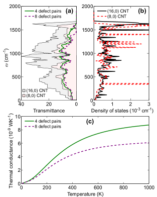
Figure 5: (a) Phonon transmittance spectra for pristine (16,0) CNT [“(16,0) CNT”], pristine (8,0) CNT [“(8,0) CNT”], the CNT IMJ with 4 heptagon-pentagon defect pairs (“4 defect pairs”), and the CNT IMJ with 8 defect pairs (“8 defect pairs”). (b) The corresponding normalized phonon density of states for pristine (16,0) and (8,0) CNTs. (c) The temperature dependence of the thermal conductances $G_{\text{4-hp}}$ (solid line) and $G_{\text{8-hp}}$ (dashed line) from 0 to 1000 K is also shown.

III.3 Modal dependence of phonon transmission

Although Fig. 5(a) yields frequency-dependent transmittance information, we cannot discern from it the modal dependence of individual phonon transmission. Instead, we use Eqs. (22) to (24) to determine the individual phonon transmission coefficients. At each frequency $\omega$, the transmission coefficient and wave vector of each propagating mode in the (16,0) CNT are determined from $\Xi_{\text{L},n}$, where $n=1,\ldots,N_{\text{L}}(+)$, in Eq. (24) and (25), respectively. The phonon mode transmission coefficients $\Xi_{\text{R},m}$, where $m=1,\ldots,N_{\text{R}}(-)$, and wave vectors in the (8,0) CNT are similarly obtained.

Figure 6(a) shows the left-lead phonon transmission coefficient sum $\sum_{n=1}^{N_{\text{L}}(+)}\Xi_{\text{L},n}$, describing the left-to-right phonon flux from the (16,0) CNT to the (8,0) CNT across the CNT IMJ with 4 and 8 heptagon-pentagon defect pairs, as well as $N_{\text{L}}(+)$ and $N_{\text{R}}(-)$ for the pristine (16,0) and (8,0) CNT, respectively. As expected from Eq. (27a), the transmission coefficient sum $\sum_{n=1}^{N_{\text{L}}(+)}\Xi_{\text{L},n}$ in Fig. 6(a) is identical to the phonon transmittance spectrum $\Xi_{n\text{-hp}}(\omega)$ in Fig. 5(a) and is also larger for the CNT IMJ with 4 heptagon-pentagon defect pairs than with 8 defect pairs. In Figs. 6(b) and (c), the numerous phonon branches associated with the phonon subband quantization of the (16,0) CNT can be seen in the phonon dispersion curves. The origin of the greater transmittance for 4 defect pairs can be discerned from Figs. 6(b) and (c) which show the transmission coefficient spectra $\Xi_{\text{L},n}$ superimposed on the phonon dispersion curves of the (16,0) CNT.

For the other side of the CNT IMJ, Fig. 6(d) shows the right-lead phonon transmission coefficient sum $\sum_{m=1}^{N_{\text{R}}(-)}\Xi_{\text{R},m}$, describing the right-to-left phonon flux from the (8,0) CNT to the (16,0) CNT, as well as $N_{\text{L}}(+)$ and $N_{\text{R}}(-)$ for the pristine (16,0) and (8,0) CNT, respectively, like in Fig. 6(a). The $\sum_{m=1}^{N_{\text{R}}(-)}\Xi_{\text{R},m}$ spectrum in Fig. 6(d) is identical to the $\sum_{n=1}^{N_{\text{L}}(+)}\Xi_{\text{L},n}$ spectrum in Fig. 6(a), in agreement with Eq. (27a). Hence, we can also explain the greater phonon transmittance for the CNT IMJ with 4 defect pairs in terms of the transmission coefficients of the (8,0) CNT phonons. Figures 6(e) and (f) show the transmission coefficient spectra $\Xi_{\text{R},m}$ superimposed on the phonon dispersion curves of the (8,0) CNT, which has fewer phonon branches than the (16,0) CNT. We find from Fig. 6(e) that most of the (8,0) CNT phonons are transmitted with a near-unity transmission coefficient. This is partly because there are fewer phonon channels contributing to the interfacial heat flux for the (8,0) CNT than in the (16,0) CNT and thus each (8,0) CNT phonon channel has to transmit on average a greater percentage of its energy across the CNT IMJ than each (16,0) CNT phonon channel. We can also tell from comparing Figs. 6(e) and (f) which phonon branches contribute more to the interfacial phonon flux for the CNT IMJ with 4 defect pairs than for the CNT IMJ with 8 defect pairs, especially given the less crowded phonon dispersion curves for the (8,0) CNT.

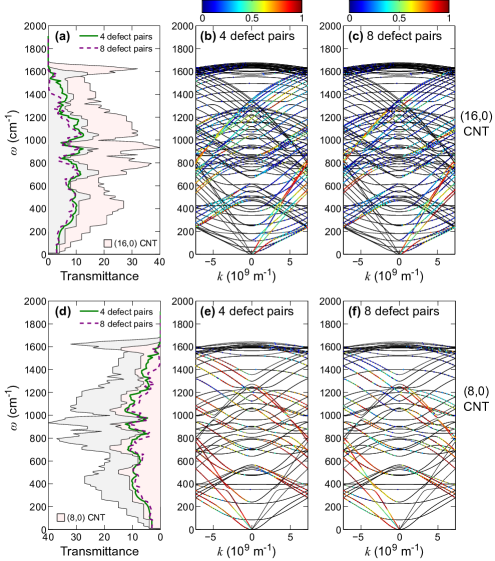
Figure 6: (a) Plot of the left-lead phonon transmission coefficient sum $\sum_{n=1}^{N_{\text{L}}(+)}\Xi_{\text{L},n}$ for the CNT IMJ with 4 (green solid line) and 8 (purple dashed line) heptagon-pentagon defect pairs, together with $N_{\text{L}}(+)$, the number of incident channels in the (16,0) CNT (pink), and $N_{\text{R}}(-)$, the number of channels in the (8,0) CNT (gray). The distribution of the transmission coefficients $\Xi_{\text{L},n}$, represented in color, is superimposed on the phonon dispersion curves of the (16,0) CNT for the CNT IMJ with (b) 4 and (c) 8 heptagon-pentagon defect pairs. (b) Plot of the right-lead phonon transmission coefficient sum $\sum_{m=1}^{N_{\text{R}}(-)}\Xi_{\text{R},m}$ for the CNT IMJ with 4 (green solid line) and 8 (purple dashed line) heptagon-pentagon defect pairs, together with $N_{\text{R}}(-)$, the number of incident channels in the (8,0) CNT (pink), and $N_{\text{L}}(+)$, the number of channels in the (16,0) CNT (gray). The distribution of the transmission coefficients $\Xi_{\text{R},m}$ is superimposed on the phonon dispersion curves of the (8,0) CNT for the CNT IMJ with (b) 4 and (c) 8 heptagon-pentagon defect pairs.

The polarization dependence of phonon transmission can also be determined from the transmission coefficient spectra. Figure 7 shows the low-frequency transmission coefficient spectra of the (16,0) and (8,0) CNT for the CNT IMJ with 4 defect pairs. At very low frequencies ($\omega\rightarrow 0$), there are four acoustic phonon branches in the carbon nanotube: the longitudinal acoustic (LA), the torsional (TW) and the doubly-degenerate transverse acoustic (TA) phonons. Our results in Fig. 7 show that the LA and TA phonons are transmitted across the interface with near unity transmission probability while the TW phonons, otherwise known as “twistons”, (Allen, 2007) are only partially transmitted with a transmission probability significantly less than 0.5. This suggests that the CNT IMJ restricts torsional motion even in the long-wavelength limit, resulting in the partial reflection of TW phonons.

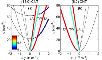
Figure 7: Plot of the low-frequency phonon transmission coefficient spectra in (a) (16,0) CNT and (b) (8,0) CNT for the CNT IMJ with 4 heptagon-pentagon defect pairs. The longitudinal (“LA”), torsional (“TW”) and transverse (“TA”) acoustic phonon branches are labelled accordingly.

IV Summary

In this tutorial, we have presented an extension of the AGF method for computing individual phonon transmission coefficients, which we summarize in Fig. 8. In the traditional AGF method, we use the input matrices ($\boldsymbol{H}_{\text{C}}$, $\boldsymbol{H}_{\text{CL}}$, $\boldsymbol{H}_{\text{CR}}$, $\boldsymbol{H}_{\text{L}}^{00}$, $\boldsymbol{H}_{\text{L}}^{01}$, $\boldsymbol{H}_{\text{R}}^{00}$ and $\boldsymbol{H}_{\text{R}}^{01}$) to compute the phonon transmittance $\Xi(\omega)$ [Eq. (9)] from the surface Green’s functions $\boldsymbol{g}_{\text{L},-}^{\text{ret}}$ and $\boldsymbol{g}_{\text{R},+}^{\text{ret}}$ [Eq. (7b)] corresponding to the decoupled leads and the retarded Green’s function of the scattering region $\boldsymbol{G}_{\text{RL}}^{\text{ret}}$ [Eq. (8)]. In our extended AGF approach, we exploit Eq. (11b) to extract the Bloch matrices $\bm{F}_{\alpha}^{\text{adv/ret}}(\pm)$ from the surface Green’s function $\boldsymbol{g}_{\alpha,\pm}^{\text{adv/ret}}$. This allows us to determine all the bulk phonon modes of the leads, $\bm{U}_{\alpha}^{\text{adv}}(\pm)$ and $\bm{U}_{\alpha}^{\text{ret}}(\pm)$ in Eq. (12b), that constitute the available incoming and outgoing transmission channels at frequency $\omega$, and their Bloch factors, $\bm{\Lambda}_{\alpha}^{\text{adv}}(\pm)$ and $\bm{\Lambda}_{\alpha}^{\text{ret}}(\pm)$. The flux-normalized transmission matrices $\boldsymbol{t}_{\text{RL}}$ and $\boldsymbol{t}_{\text{LR}}$ which govern the transition probability between each pair of incoming and outgoing phonon channels can be computed from Eqs. (22) and (23). The single-mode transmission coefficients $\Xi_{\text{L},n}$, which determines the phonon transmission probability, can be computed from Eq. (24). The extended AGF method provides a clear and detailed view of the contribution of individual phonon modes as well as that of entire acoustic and optical phonon branches to the thermal boundary conductance. It is a powerful and convenient method for analyzing the effect of the atomistic structure of the interface on the contribution of individual phonon modes to interfacial thermal transport.

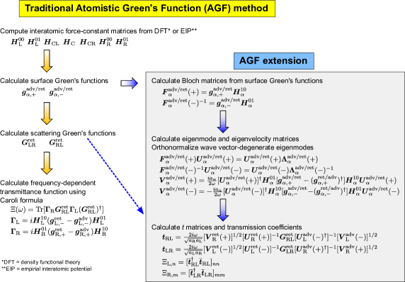
Figure 8: Flow chart summarizing the main steps in the traditional AGF method and its extension (enclosed in a gray subpanel) for computing transmission coefficients.

We use the simple example of a linear atomic chain junction to demonstrate the basic ideas of the extended AGF method as well as to highlight the connection between the phonon transmission coefficients and the phonon transmittance as calculated with traditional AGF technique. To illustrate the advantages of the extended AGF method for realistic material systems, we have applied it to the study of thermal conduction across the (16,0)/(8,0) carbon nanotube intramolecular junction. Our analysis of phonon transmission across the CNT IMJ shows that the transmission probability depends strongly on the CNT phonon frequency, polarization and wave vector as well as the atomistic configuration of the interface (i.e. the number of heptagon-pentagon defect pairs). Our AGF simulation results suggest that phonon are more easily transmitted across the CNT IMJ with 4 defect pairs than with 8 defect pairs, in agreement with the findings of Ref. (Wu and Li, 2007). They also demonstrate how the extended AGF method can play synergistic role to other simulation-based approaches to thermal transport.