Testing the multipole structure of compact binaries using gravitational wave observations

Abstract

We propose a novel method to test the consistency of the multipole moments of compact binary systems with the predictions of general relativity (GR). The multipole moments of a compact binary system, known in terms of symmetric and trace-free tensors, are used to calculate the gravitational waveforms from compact binaries within the post-Newtonian (PN) formalism. For nonspinning compact binaries, we derive the gravitational wave phasing formula, in the frequency domain, parametrizing each PN order term in terms of the multipole moments which contribute to that order. Using GW observations, this parametrized multipolar phasing would allow us to derive the bounds on possible departures from the multipole structure of GR and hence constrain the parameter space of alternative theories of gravity. We compute the projected accuracies with which the second-generation ground-based detectors, such as the Advanced Laser Interferometer Gravitational-wave Observatory (LIGO), the third-generation detectors such as the Einstein Telescope and Cosmic Explorer, as well as the space-based detector Laser Interferometer Space Antenna (LISA) will be able to measure these multipole parameters. We find that while Advanced LIGO can measure the first two or three multipole coefficients with good accuracy, Cosmic Explorer and the Einstein Telescope may be able to measure the first four multipole coefficients which enter the phasing formula. Intermediate-mass-ratio inspirals, with mass ratios of several tens, in the frequency band of the planned space-based LISA mission should be able to measure all seven multipole coefficients which appear in the 3.5PN phasing formula. Our finding highlights the importance of this class of sources for probing the strong-field gravity regime. The proposed test will facilitate the first probe of the multipolar structure of Einstein’s general relativity.

I Introduction

The discovery of binary black holes Abbott et al. (2016a, b, 2017a, 2017b) and binary neutron stars Abbott et al. (2017c) by Advanced LIGO Collaboration et al. (2015) and Advanced Virgo Acernese et al. (2015) have been ground breaking for several reasons. Among the most important aspects of these discoveries is the unprecedented opportunity they have provided to study the behavior of gravity in the highly nonlinear and dynamical regime associated with the merger of two black holes (BHs) or two neutron stars (see Refs. Sathyaprakash and Schutz (2009); Yunes and Siemens (2013) for reviews). The gravitational wave (GW) observations have put stringent constraints on the allowed parameter space of alternative theories of gravity by different methods Abbott et al. (2016c, d, 2017a). They include the parametrized tests of post-Newtonian theory Arun et al. (2006a, b); Yunes and Pretorius (2009); Mishra et al. (2010); Agathos et al. (2014); Li et al. (2012); Meidam et al. (2018), bounding the mass of the putative graviton and dispersion of GWs Will (1998); Mirshekari et al. (2012), testing consistency between the inspiral and ringdown regimes of the coalescence Ghosh et al. (2016) and the time delay between the GW and electromagnetic signals Abbott et al. (2017d). Furthermore, the bounds obtained from these tests have been translated into bounds on the free parameters of certain specific theories of gravity Yunes et al. (2016).

With improved sensitivities of Advanced LIGO and Virgo in the upcoming observing runs, the development of third-generation detectors such as the Einstein Telescope (ET) Abernathy et al. (2010) and Cosmic Explorer (CE) Abbott et al. (2017e) and the approval of funding for the space-based mission LISA LIS , the field of gravitational astronomy promises to deliver exciting science returns. In addition to stellar-mass compact binaries, future ground-based detectors, such as ET and CE, can detect intermediate-mass black holes with a total mass of several hundreds of solar masses. Such observations will not only confirm the existence of BHs in this mass range (see Refs. Miller and Colbert (2004); van der Marel (2003) for reviews), but also facilitate several new probes of fundamental physics via studying their dynamics Fregeau et al. (2006); Graff et al. (2015); Brown et al. (2007); Chamberlain and Yunes (2017). Some of the most prominent, among these, are those using intermediate-mass-ratio inspirals, which will last longer (compared to the equal-mass binaries), and hence are an accurate probe of the compact binary dynamics and the BH nature of the central compact object Ryan (1997); Brown et al. (2007).

The space-based LISA mission, on the other hand, will be sensitive to millihertz GWs produced by the inspirals and merger of supermassive BH binaries in the mass range $\sim 10^{4}$-$10^{7}M_{\odot}$. These sources may also have a large diversity in their mass ratios ranging from comparable mass (mass ratio $\lesssim 10$) and intermediate mass ratios (mass ratio $\gtrsim 100$) to extreme mass ratios (mass ratio $\gtrsim 10^{6}$) where a stellar mass BH spirals into the central supermassive BH with several millions of solar masses Thorne (1995); Schutz (1996). This diversity together with the sensitivity in the low-frequency window makes LISA a very efficient probe of possible deviations from general relativity (GR) in different regimes of dynamics (see Refs. Gair et al. (2013); Berti et al. (2015); Sathyaprakash and Schutz (2009); Arun and Pai (2013) for reviews).

Setting stringent limits on possible departures from GR as well as constraining the parameter space of exotic compact objects that can mimic the properties of BHs Giudice et al. (2016); Chirenti and Rezzolla (2016); Cardoso et al. (2016, 2017); Johnson-Mcdaniel et al. (2018); Krishnendu et al. (2017); Dhanpal et al. (2018); Krishnendu et al. (2018), are among the principle science goals of the next-generation detectors. They should also be able to detect any new physics, or modifications to GR, if present.

Formulating new methods to carry out such tests is crucial in order to efficiently extract the physics from GW observations. The dynamics of a compact binary system is conventionally divided into the adiabatic inspiral, rapid merger and fast ringdown phases. During the inspiral phase the orbital time scale is much smaller than the radiation backreaction time scale. The post-Newtonian (PN) approximation to GR has proved to be a very effective method to describe the inspiral phase of a compact binary of comparable masses Blanchet (2014). A description of the highly nonlinear phase of the merger of two compact objects needs numerical solutions to Einstein’s equations Pretorius (2007). The ringdown radiation of GWs by the merger remnant, can be modeled within the framework of BH perturbation theory Sasaki and Tagoshi (2003). In alternative theories of gravity, the dynamics of the compact binary during these phases of evolution could be quite different from that predicted by GR. Hence observing GWs is the best way to probe the presence of non-GR physics associated with this phenomenon.

One of the most generic tests of the binary dynamics has been the measurement of the PN coefficients of the GW phasing formula Blanchet and Sathyaprakash (1994, 1995); Arun et al. (2006a, b); Yunes and Pretorius (2009); Mishra et al. (2010); Agathos et al. (2014). This test captures a possible departure from GR by measuring the PN coefficients in the phase evolution of the GW signal. In addition to the source physics, the different PN terms in the phase evolution contain information about different nonlinear interactions the wave undergoes as it propagates from the source to the detector. Hence the predictions for these effects in an alternative theory of gravity could be very different from that of GR, which is what is being tested using the parametrized tests of PN theory.

In this work, we go one step further and propose a novel way to test the multipolar structure of the gravitational field of a compact binary as it evolves through the adiabatic inspiral phase. The multipole moments of the compact binary (and interactions between them), are responsible for the various physical effects we see at different PN orders. By measuring these effects we can constrain the multipolar structure of the system. The GW phase and frequency evolution is obtained from the energy flux of GWs and the conserved orbital energy by using the energy balance argument, which equates the GW energy flux ${\cal F}$ to the decrease in the binding energy $E_{\rm orb}$ of the binary Blanchet et al. (1995a)

$${\cal F}=-\frac{d}{dt}E_{\rm orb}.$$ (1)

In an alternative theory of gravity, one or more multipole moments of a binary system may be different from those of GR. For instance, in Ref. Endlich et al. (2017), the authors discuss how effective-field-theory-based approach can be used to go beyond Einstein’s gravity by introducing additional terms to the GR Lagrangian which are higher-order operators constructed out of the Riemann tensor, but suppressed by appropriate scales comparable to the curvature of the compact binaries. They find that such generic modifications will lead to multipole moments of compact binaries that are different from GR. Our proposed method aims to constrain such generic extensions of GR by directly measuring the multipole moments of the compact binaries through GW observations.

In this work, we assume that the conserved orbital energy of the binary is the same as in GR and modify the gravitational wave flux by deforming the multipole moments which contribute to it by employing the multipolar post-Minkowskian formalism Blanchet (2014); Blanchet et al. (1995a). We then rederive the GW phase and its frequency evolution (sometimes referred to as the phasing formula) explicitly in terms of the various deformed multipole moments (In the Appendix we provide a more general expression for the phasing where the conserved energy is also deformed at different PN orders, in addition to the multipole moments of the source.). We use this parametrized multipolar phasing formula to measure possible deviations from GR and discuss the level of bounds we can expect from the current and next-generation ground-based GW detectors, as well as the space-based LISA detector. We obtain the measurement accuracy of the system’s physical parameters and the deformation of the multipole moments using the semianalytical Fisher information matrix Rao (1945); Cramer (1946). These results are validated for several configurations of the binary system by Markov chain Monte Carlo (MCMC) sampling of the likelihood function using the emcee Foreman-Mackey et al. (2013) algorithm.

We find that Advanced LIGO-like detectors can constrain at most two of the leading multipoles, while a third-generation detector, such as ET or CE, can set constraints on as many as four of the leading multipoles. The space-based LISA detector will have the ability to set good limits on all seven multipole moments that contribute to the 3.5PN phasing formula, making it a very accurate probe of the highly nonlinear dynamics of compact binaries.

The organization of the paper is as follows. In Sec. II we describe the basic formalism to obtain the parametrized multipolar GW phasing formula. In Sec. III we briefly explain the two parameter estimation schemes (Fisher information matrix and Bayesian inference) used in our analysis, followed by Sec. IV where we discuss the results we obtain for various ground-based and space-based detectors. Section V summarizes the paper and lists some of the follow-ups we are pursuing.

II Parametrized multipolar gravitational wave phasing

The two-body problem in GR can be solved perturbatively using PN theory in the adiabatic regime, where the orbital time scale is much smaller than the radiation backreaction time scale (see Ref. Blanchet (2014) for a review). The PN theory has given us several useful insights about various facets of the two-body dynamics and the resulting gravitational radiation.

In the multipolar post-Minkowskian (MPM) formalism Thorne (1980); Blanchet and Damour (1984, 1986); Blanchet (1987); Blanchet and Damour (1988a, 1989, 1992); Blanchet (1995); Blanchet et al. (1995a, 2002a); Damour et al. (2001a); Blanchet et al. (2004a), the important quantities such as the gravitational waveform, energy and angular momentum fluxes can be expressed using a combination of post-Minkowskian approximation (expansion in powers of $G$, Newton’s gravitational constant, valid throughout the spacetime for weakly gravitating sources), PN expansions (an expansion in ${1/c}$ that is valid for slowly moving and weakly gravitating sources and applicable in the near zone of the source) and the multipole expansion of the gravitational field valid over the entire region exterior to the source. The coefficients of post-Minkowskian expansion and the multipole moments of the source can be further expanded as a PN series. The multipole expansion of the gravitational field plays a central role in the analytical treatment of the two-body problem as it significantly helps to handle the nonlinearities of Einstein’s equations.

The MPM formalism relates the radiation content in the far zone (at the detector) to the stress-energy tensor of the source. The quantities in the far zone are described by mass- and current-type radiative multipole moments $\{U_{L},V_{L}\}$ whereas the properties of the source are completely described by the mass- and current-type source multipole moments $\{I_{L},J_{L}\}$ and the four gauge moments $\{W_{L},X_{L},Y_{L},Z_{L}\}$ all of which are the moments of the relativistic mass and current densities expressed as functionals of the stress-energy pseudo-tensor of the source and gravitational fields. However, in GR, there is further gauge freedom to reduce this set of six source moments to a set of two “canonical” multipole moments $\{M_{L},S_{L}\}$. The relations connecting these two sets of multipole moments can be found in Eqs. (97) and (98) of Ref. Blanchet (2014). Furthermore, the mass- and current-type radiative multipole moments $\{U_{L},V_{L}\}$ admit closed-form expressions in terms of $\{M_{L},S_{L}\}$.

The source and the canonical multipole moments are usually expressed using the basis of symmetric trace-free tensors Damour and Iyer (1991). The relationships between the radiative- and source-type multipole moments incorporate the various nonlinear interactions between the various multipoles, such as tails Blanchet and Damour (1988b); Blanchet and Schaefer (1993); Blanchet et al. (1995a), tails of tails Blanchet (1998a), tail square Blanchet (1998b), memory Christodoulou (1991); Thorne (1992); Arun et al. (2004); Favata (2009), $\ldots,$ as the wave propagates from the source to the detector (see Ref. Blanchet (2014) for more details).

For quasicircular inspirals, the PN expressions for the orbital energy and the energy flux, together with the energy balance argument is used in the computation of the GW phasing formula at any PN order Blanchet et al. (1995a, b, 2002b, 2004a). The PN terms in the phasing formula, hence, explicitly encode the information about the multipolar structure of the gravitational field of the two-body dynamics.

In this work, we separately keep track of the contributions from various radiative multipole moments to the GW flux allowing us to derive a parametrized multipolar gravitational wave flux and phasing formula, thereby permitting tests of the multipolar structure of the PN approximation to GR. We first rederive the phasing formula for nonspinning compact binaries moving in quasicircular orbits up to 3.5 PN order. The computation is described in the next section. Before we proceed, we clarify that in our notation the first post-Newtonian (1PN) correction would refer to corrections of order $v^{2}/c^{2}$, where $v=(\pi mf)^{1/3}$ is the characteristic orbital velocity of the binary, $m$ is the total mass of the binary and $f$ is the orbital frequency.

II.1 The multipolar structure of the energy flux

The multipole expansion of the energy flux within the MPM formalism schematically reads as Thorne (1980); Blanchet et al. (1995a)

$${\cal F}=\sum_{l}\left[\frac{\alpha_{l}}{c^{l-2}}U_{L}^{(1)}U_{L}^{(1)}+\frac{\beta_{l}}{c^{l}}V_{L}^{(1)}V_{L}^{(1)}\right],$$ (2)

where $\alpha_{l},\beta_{l}$ are known real numbers and $U_{L},V_{L}$ are mass- and current-type radiative multipole moments with $l$ indices; the superscript $(1)$ denotes the first time derivative of the multipoles. The $U_{L}$ and $V_{L}$ can be rewritten in terms of the source multipole moments as

$$U_{L}=M_{L}^{(l)}+{\rm Nonlinear\;interaction\;terms},$$ (3)

$$V_{L}=S_{L}^{(l)}+{\rm Nonlinear\;interaction\;terms},$$ (4)

where the right-hand side involves $l^{\rm th}$ time derivative of the mass- and current-type source multipole moments and nonlinear interactions between the various multipoles due to the propagation of the wave in the curved spacetime of the source. (see Refs. Blanchet and Damour (1992); Blanchet (1998b, a); Blanchet et al. (2002a) for details). The various types of interactions can be decomposed as follows Blanchet et al. (1995a, 2002a)

$$\mathcal{F}=\mathcal{F}_{\mathrm{inst}}+\mathcal{F}_{\mathrm{tail}}+\mathcal{F}_{\mathrm{tail}^{2}}+\mathcal{F}_{\mathrm{tail}(\mathrm{tail})}.$$ (5)

As opposed to $\mathcal{F}_{\mathrm{inst}}$ (a contribution that depends on the dynamics of the binary at the purely retarded instant of time, referred to as instantaneous terms), the last three contributions $\mathcal{F}_{\mathrm{tail}}$, $\mathcal{F}_{\mathrm{tail}^{2}}$ and $\mathcal{F}_{\mathrm{tail}(\mathrm{tail})}$ contain nonlinear multipolar interactions in the flux Blanchet (1998a) that depend on the dynamical history of the system and are referred to as hereditary contributions.

In an alternative theory of gravity, the multipole moments may not be the same as in GR; if the mass- and current-type radiative multipole moments deviate from their GR values by a fractional amount $\delta U_{L}$ and $\delta V_{L},$ i.e., $U_{L}\rightarrow U_{L}^{\rm GR}+\delta U_{L}$ and $V_{L}\rightarrow V_{L}^{\rm GR}+\delta V_{L}$, then we can parametrize such deviations in the multipoles by considering the scalings

$$U_{L}\rightarrow\mu_{l}\,U_{L},$$

$$V_{L}\rightarrow\epsilon_{l}\,V_{L},$$ (6)

where the parameters $\mu_{l}=1+\delta U_{L}/U_{L}^{\rm GR}$ and $\epsilon_{l}=1+\delta V_{L}/V_{L}^{\rm GR}$ are equal to unity in GR.

We first recompute the GW flux from nonspinning binaries moving in quasicircular orbit up to 3.5PN order with the above scaling using the prescription outlined in Refs. Blanchet et al. (1995a); Blanchet (1995); Blanchet et al. (2002a, 2004a). With the parametrizations introduced above, the computation of the energy flux would proceed similarly to that in GR but contributions from every radiative multipole are now separately kept track of.

In order to calculate the fluxes up to the required PN order, we need to compute the time derivatives of the multipole moments as can be seen from Eqs. (2-(4). These are computed by using the equations of motion of the compact binary for quasicircular orbits given by Blanchet and Iyer (2003); Blanchet et al. (2002a)

$$\frac{d{\bf v}}{dt}=-\omega^{2}\,{\bf x},$$ (7)

where the expression for $\omega$, the angular frequency of the binary, up to 3PN order is given by Damour et al. (2001a); Blanchet et al. (2004b); Damour et al. (2001b); de Andrade et al. (2001); Blanchet and Iyer (2003); Itoh and Futamase (2003); Blanchet et al. (2002b)

$$\omega^{2} = {Gm\over r^{3}}\Biggl{\{}1+\left[-3+\nu\right]\gamma+\left[6+{41\over 4}\nu+\nu^{2}\right]\gamma^{2}$$ (8)

$$+ \left[-10+\left(22\ln\left(r\over{r^{\prime}}_{0}\right)+{41\pi^{2}\over 64}-{75707\over 840}\right)\nu\right.$$

$$+ \left.{19\over 2}\nu^{2}+\nu^{3}\right]\gamma^{3}+{\cal O}(\gamma^{4})\Biggr{\}},$$

where $\gamma=Gm/rc^{2}$ is a PN parameter, $r_{0}^{\prime}$ is a gauge-dependent length scale which does not appear when observables, such as the energy flux, are expressed in terms of gauge-independent variables.

The hereditary terms are calculated using the prescriptions given in Refs. Blanchet and Schaefer (1993); Blanchet et al. (1995a); Blanchet (1996); Blanchet et al. (2002a) for tails, Ref. Blanchet (1998a) for tails of tails and Ref. Blanchet (1998b) for tail square. The complete expression for the energy flux ${\cal F}$ in terms of the scaled multipoles is given as

$$\mathcal{F}= \frac{32}{5}\frac{c^{5}v^{10}}{G}\nu^{2}\mu_{2}^{2}\Bigg{\{}1+v^{2}\Bigg{(}-\frac{107}{21}+\frac{55}{21}\nu+{\hat{\mu}}_{3}^{2}\Bigg{[}\frac{1367}{1008}-\frac{1367}{252}\nu\Bigg{]}+\hat{\epsilon_{2}}^{2}\Bigg{[}\frac{1}{36}-\frac{\nu}{9}\Bigg{]}\Bigg{)}+4\pi v^{3}+v^{4}\Bigg{(}\frac{4784}{1323}-\frac{87691}{5292}\nu$$ (9)

$$+\frac{5851}{1323}\nu^{2}+\hat{\mu}_{3}^{2}\Bigg{[}-\frac{32807}{3024}+\frac{3515}{72}\nu-\frac{8201}{378}\nu^{2}\Bigg{]}+\hat{\mu}_{4}^{2}\Bigg{[}\frac{8965}{3969}-\frac{17930}{1323}\nu+\frac{8965}{441}\nu^{2}\Bigg{]}+\hat{\epsilon_{2}}^{2}\Bigg{[}-\frac{17}{504}+\frac{11}{63}\nu-\frac{10}{63}\nu^{2}\Bigg{]}$$

$$+\hat{\epsilon_{3}}^{2}\Bigg{[}\frac{5}{63}-\frac{10}{21}\nu+\frac{5}{7}\nu^{2}\Bigg{]}\Bigg{)}+\pi v^{5}\Bigg{(}-\frac{428}{21}+\frac{178}{21}\nu+\hat{\mu}_{3}^{2}\Bigg{[}\frac{16403}{2016}-\frac{16403}{504}\nu\Bigg{]}+\hat{\epsilon_{2}}^{2}\Bigg{[}\frac{1}{18}-\frac{2}{9}\nu\Bigg{]}\Bigg{)}$$

$$+v^{6}\Bigg{(}\frac{99210071}{1091475}+\frac{16\pi^{2}}{3}-\frac{1712}{105}\gamma_{E}-\frac{856}{105}\log[16v^{2}]+\Bigg{[}\frac{1650941}{349272}+\frac{41\pi^{2}}{48}\Bigg{]}\nu-\frac{669017}{19404}\nu^{2}+\frac{255110}{43659}\nu^{3}$$

$$+\hat{\mu}_{3}^{2}\Bigg{[}\frac{7345}{297}-\frac{30103159}{199584}\nu+\frac{10994153}{49896}\nu^{2}-\frac{45311}{891}\nu^{3}\Bigg{]}+\hat{\mu}_{4}^{2}\Bigg{[}-\frac{1063093}{43659}+\frac{20977942}{130977}\nu-\frac{12978200}{43659}\nu^{2}$$

$$+\frac{1568095}{14553}\nu^{3}\Bigg{]}+\hat{\mu}_{5}^{2}\Bigg{[}\frac{1002569}{249480}-\frac{1002569}{31185}\nu+\frac{1002569}{12474}\nu^{2}-\frac{2005138}{31185}\nu^{3}\Bigg{]}+\hat{\epsilon}_{2}^{2}\Bigg{[}-\frac{2215}{254016}-\frac{13567}{63504}\nu+\frac{65687}{63504}\nu^{2}$$

$$-\frac{853\nu^{3}}{5292}\Bigg{]}+\hat{\epsilon_{3}}^{2}\Bigg{[}-\frac{193}{567}+\frac{1304}{567}\nu-\frac{2540}{567}\nu^{2}+\frac{365}{189}\nu^{3}\Bigg{]}+\hat{\epsilon_{4}}^{2}\Bigg{[}\frac{5741}{35280}-\frac{5741}{4410}\nu+\frac{5741}{1764}\nu^{2}-\frac{5741}{2205}\nu^{3}\Bigg{]}\Bigg{)}$$

$$+\pi v^{7}\Bigg{(}\frac{19136}{1323}-\frac{144449}{2646}\nu+\frac{33389}{2646}\nu^{2}+\hat{\mu}_{3}^{2}\Bigg{[}-\frac{98417}{1512}+\frac{55457}{192}\nu-\frac{344447}{3024}\nu^{2}\Bigg{]}+\hat{\mu}_{4}^{2}\Bigg{[}\frac{23900}{1323}-\frac{47800}{441}\nu$$

$$+\frac{23900}{147}\nu^{2}\Bigg{]}+\hat{\epsilon_{2}}^{2}\Bigg{[}-\frac{17}{252}+\frac{9}{28}\nu-\frac{13}{63}\nu^{2}\Bigg{]}+\hat{\epsilon_{3}}^{2}\Bigg{[}\frac{20}{63}-\frac{40}{21}\nu+\frac{20}{7}\nu^{2}\Bigg{]}\Bigg{)}\Bigg{\}},$$

where $\hat{\mu}_{\ell}=\mu_{\ell}/\mu_{2}$, $\hat{\epsilon_{\ell}}=\epsilon_{\ell}/\mu_{2}$, Euler constant, $\gamma_{E}=0.577216$ and $\nu$ is the symmetric mass ratio defined as the ratio of reduced mass $\mu$ to the total mass $m$. As an algebraic check of the result, we recover the GR results of Ref. Blanchet et al. (2002a) in the limit $\mu_{l}\rightarrow 1,\epsilon_{l}\rightarrow 1.$

II.2 Conservative dynamics of the binary

A model for the conservative dynamics of the binary is also required to compute the phase evolution of the system. This enters the phasing formula in two ways. First, the equation of motion of the binary Blanchet and Iyer (2003) in the center-of-mass frame is required to compute the derivatives of the multipole moments while calculating the energy flux. Second, the expression for the 3PN orbital energy Blanchet and Iyer (2003); Blanchet et al. (2002b) is necessary to compute the equation of energy balance to obtain the phase evolution [see Eqs. (14)–(15) below]. As the computation of the radiative multipole moments requires two or more derivative operations, they are implicitly sensitive to the equation of motion. Hence, formally, a constraint on the deformation of the radiative multipole moment does take into account a potential deviation in the equation of motion from the predictions of GR.

Here however we assume that the conserved energy is the same as in GR. This assumption is motivated by practical considerations. We could have taken a more generic approach by deforming the PN coefficients in the equation of motion and conserved energy as well. As the former is degenerate with the definition of radiative multipole moments, one would need to consider a parametrized expression for the conserved energy which will give us a phasing formula with four additional parameters corresponding to the different PN orders in the expression for conserved energy. A simultaneous estimation of these parameters with the multipole coefficients would significantly degrade the resulting bounds and may not yield meaningful constraints. However, in the Appendix, we present a parametrized phasing formula where in addition to the multipole coefficients, various PN-order terms in the conserved 3PN energy expression are also deformed [see Eq. (27) below]. Interestingly, as can be seen from Eq. (27), if there is a modification to the conservative dynamics, they will be fully degenerate with at least one of the multipole coefficients appearing at the same order. Due to this degeneracy, such modifications will be detected by this test as modifications to “effective” multipole moments. Further, this degeneracy is not accidental. It can be shown that by differentiating the expression for the conserved energy, one can derive the energy flux by systematically accounting for the equation of motion, including radiation reaction terms Iyer and Will (1993, 1995). We are, therefore, confident that the power of the proposed test is not diminished by this assumption. The conserved energy (per unit mass) up to 3PN order is given by Damour et al. (2001a, b); Blanchet et al. (2004b); de Andrade et al. (2001); Blanchet and Iyer (2003); Itoh and Futamase (2003); Blanchet et al. (2002b)

$$E(v) = -\frac{1}{2}\nu v^{2}\left[1-\left(\frac{3}{4}+\frac{1}{12}\nu\right)v^{2}-\left(\frac{27}{8}-\frac{19}{8}\nu+\frac{1}{24}\nu^{2}\right)v^{4}\right.$$ (10)

$$\left.-\left\{\frac{675}{64}-\left(\frac{34445}{576}-\frac{205}{96}\pi^{2}\right)\nu+\frac{155}{96}\nu^{2}\right.\right.$$

$$\left.\left.+\frac{35}{5184}\nu^{3}\right\}v^{6}\right]\,.$$

Using the expressions for the modified flux and the orbital energy we next proceed to compute the phase evolution of the compact binary.

II.3 Computation of the parametrized multipolar phasing formula

With the parametrized multipolar flux and the energy expressions, we compute the 3.5PN, nonspinning, frequency-domain phasing formula following the standard prescription Damour et al. (2000); Buonanno et al. (2009) by employing the stationary phase approximation (SPA) Sathyaprakash and Dhurandhar (1991). Consider a GW signal of the form

$$h(t)=\mathcal{A}(t)\cos{\phi(t)}.$$ (11)

The Fourier transform of the signal will involve an integrand whose amplitude is slowly varying and whose phase is rapidly oscillating. In the SPA, the dominant contributions to this integral come from the vicinity of the stationary points of its phase Damour et al. (2000). As a result the frequency-domain gravitational waveform may be expressed as

$$\tilde{h}^{\text{SPA}}(f) =\frac{\mathcal{A}(t_{f})}{\sqrt{\dot{F}(t_{f})}}e^{i[\psi_{f}(t_{f})-\pi/4]}\,,$$ (12)

$$\psi_{f}(t) =2\pi ft-\phi(t),$$ (13)

where $t_{f}$ can be obtained by solving $\left.d\psi_{f}(t)/dt\right|_{t_{f}}=0$, $F(t)$ is the gravitational wave frequency and at $t=t_{f}$ the GW frequency coincides with the Fourier variable $f$. More explicitly,

$$t_{f} = t_{\text{ref}}+m\int_{v_{f}}^{v_{ref}}\frac{E^{\prime}(v)}{\mathcal{F}(v)}dv\,,$$ (14)

$$\psi_{f}(t_{f}) = 2\pi ft_{\text{ref}}-\phi_{\text{ref}}+2\int_{v_{f}}^{v_{ref}}(v_{f}^{3}-v^{3})\frac{E^{\prime}(v)}{\mathcal{F}(v)}dv,$$ (15)

where $E^{\prime}(v)$ is the derivative of the binding energy of the system expressed in terms of the PN expansion parameter $v$. Expanding the factor in the integrand in Eq. (15) as a PN series and truncating up to 3.5PN order, we obtain the 3.5PN accurate TaylorF2 phasing formula.

Following the very same procedure, but using Eq. (9) to be the parametrized flux, $\mathcal{F}$, together with the leading quadrupolar order amplitude (related to the Newtonian GW polarizations), we derive the standard restricted PN waveform in the frequency domain, which reads as

$$\tilde{h}(f)=\mathcal{A}\,\mu_{2}\,f^{-7/6}e^{i\psi(f)},$$ (16)

where $\psi(f)$ is the parametrized multipolar phasing, $\mathcal{A}=\mathcal{M}_{c}^{5/6}/\sqrt{30}\pi^{2/3}D_{L}$; $\mathcal{M}_{c}=(m_{1}m_{2})^{3/5}/(m_{1}+m_{2})^{1/5}$ and $D_{L}$ are the chirp mass and luminosity distance, respectively, and $m_{1},m_{2}$ denote the component masses of the binary. Note the presence of $\mu_{2}$ in the GW amplitude, this is due to the mass quadrupole that contributes to the amplitude at the leading PN order. If we incorporate the higher-order PN terms in the GW polarizations Blanchet et al. (1996); Arun et al. (2004); Blanchet et al. (2008), higher-order multipoles will enter the GW amplitude as well.

Finally the expression for the 3.5PN frequency-domain phasing $\psi(f)$ is given by,

$$\psi(f) = 2\pi ft_{c}-\frac{\pi}{4}-\phi_{c}+\frac{3}{128v^{5}\mu_{2}^{2}\nu}\Bigg{\{}1+v^{2}\Bigg{(}\frac{1510}{189}-\frac{130}{21}\nu+\hat{\mu}_{3}^{2}\Bigg{[}-\frac{6835}{2268}+\frac{6835}{567}\nu\Bigg{]}+\hat{\epsilon_{2}}^{2}\Bigg{[}-\frac{5}{81}+\frac{20}{81}\nu\Bigg{]}\Bigg{)}$$ (17)

$$-16\pi v^{3}+v^{4}\Bigg{(}\frac{242245}{5292}+\frac{4525}{5292}\nu+\frac{145445}{5292}\nu^{2}+{\hat{\mu}_{3}}^{2}\Bigg{[}-\frac{66095}{7056}+\frac{170935}{3024}\nu-\frac{403405}{5292}\nu^{2}\Bigg{]}+{\hat{\mu}_{3}}^{2}\hat{\epsilon_{2}}^{2}\Bigg{[}\frac{6835}{9072}$$

$$-\frac{6835}{1134}\nu+\frac{6835\nu^{2}}{567}\Bigg{]}+\hat{\mu}_{3}^{4}\Bigg{[}\frac{9343445}{508032}-\frac{9343445}{63504}\nu+\frac{9343445}{31752}\nu^{2}\Bigg{]}+\hat{\mu}_{4}^{2}\Bigg{[}-\frac{89650}{3969}+\frac{179300}{1323}\nu-\frac{89650}{441}\nu^{2}\Bigg{]}$$

$$+\hat{\epsilon_{2}}^{2}\Bigg{[}-\frac{785}{378}+\frac{7115}{756}\nu-\frac{835}{189}\nu^{2}\Bigg{]}+\hat{\epsilon_{2}}^{4}\Bigg{[}\frac{5}{648}-\frac{5}{81}\nu+\frac{10}{81}\nu^{2}\Bigg{]}+\hat{\epsilon_{3}}^{2}\Bigg{[}-\frac{50}{63}+\frac{100}{21}\nu-\frac{50}{7}\nu^{2}\Bigg{]}\Bigg{)}$$

$$+\pi v^{5}\Big{(}3\log\left[\frac{v}{v_{\rm LSO}}\right]+1\Big{)}\Bigg{(}\frac{80}{189}\Big{[}151-138\nu\Big{]}-\frac{9115}{756}\hat{\mu}_{3}^{2}\Big{[}1-4\nu\Big{]}-\frac{20}{27}\hat{\epsilon_{2}}^{2}\Big{[}1-4\nu\Big{]}\Bigg{)}+v^{6}\Bigg{(}\frac{5334452639}{2037420}$$

$$-\frac{640}{3}\pi^{2}-\frac{6848}{21}\gamma_{E}-\frac{6848}{21}\log[4v]-\Bigg{[}\frac{7153041685}{1222452}-\frac{2255}{12}\pi^{2}\Bigg{]}\nu+\frac{123839990}{305613}\nu^{2}+\frac{18300845}{1222452}\nu^{3}$$

$$+\hat{\mu}_{3}^{2}\Bigg{[}-\frac{4809714655}{29338848}+\frac{8024601785}{9779616}\nu-\frac{19149203695}{29338848}\nu^{2}-\frac{190583245}{7334712}\nu^{3}\Bigg{]}+\hat{\mu}_{3}^{2}\hat{\epsilon_{2}}^{2}\Bigg{[}-\frac{656195}{95256}+\frac{229475\nu}{3888}$$

$$-\frac{3369935\nu^{2}}{23814}+\frac{82795\nu^{3}}{1323}\Bigg{]}+\hat{\mu}_{3}^{2}\hat{\epsilon_{2}}^{4}\Bigg{[}\frac{6835}{108864}-\frac{6835}{9072}\nu+\frac{6835}{2268}\nu^{2}-\frac{6835}{1701}\nu^{3}\Bigg{]}+\hat{\mu}_{3}^{2}\hat{\epsilon_{3}}^{2}\Bigg{[}-\frac{34175}{7938}+\frac{170875}{3969}\nu$$

$$-\frac{375925}{2646}\nu^{2}+\frac{68350}{441}\nu^{3}\Bigg{]}+\hat{\mu}_{3}^{2}\hat{\mu}_{4}^{2}\Bigg{[}-\frac{61275775}{500094}+\frac{306378875}{250047}\nu-\frac{674033525}{166698}\nu^{2}+\frac{122551550}{27783}\nu^{3}\Bigg{]}$$

$$+\hat{\mu}_{3}^{4}\Bigg{[}\frac{868749005}{10668672}-\frac{2313421945}{3556224}\nu+\frac{191974645}{148176}\nu^{2}+\frac{9726205}{666792}\nu^{3}\Bigg{]}+\hat{\mu}_{3}^{4}\hat{\epsilon_{2}}^{2}\Bigg{[}\frac{9343445}{3048192}-\frac{9343445}{254016}\nu$$

$$+\frac{9343445}{63504}\nu^{2}-\frac{9343445}{47628}\nu^{3}\Bigg{]}+\hat{\mu}_{3}^{6}\Bigg{[}\frac{12772489315}{256048128}-\frac{12772489315}{21337344}\nu+\frac{12772489315}{5334336}\nu^{2}-\frac{12772489315}{4000752}\nu^{3}\Bigg{]}$$

$$+\hat{\mu}_{4}^{2}\Bigg{[}-\frac{86554310}{916839}+\frac{553387330}{916839}\nu-\frac{289401650}{305613}\nu^{2}-\frac{4322750}{101871}\nu^{3}\Bigg{]}+\hat{\mu}_{4}^{2}\hat{\epsilon_{2}}^{2}\Bigg{[}-\frac{89650}{35721}+\frac{896500}{35721}\nu$$

$$-\frac{986150}{11907}\nu^{2}+\frac{358600\nu^{3}}{3969}\Bigg{]}+\hat{\mu}_{5}^{2}\Bigg{[}\frac{1002569}{12474}-\frac{4010276}{6237}\nu+\frac{10025690}{6237}\nu^{2}-\frac{8020552}{6237}\nu^{3}\Bigg{]}$$

$$+\hat{\epsilon_{2}}^{2}\Bigg{[}\frac{3638245}{190512}-\frac{2842015}{31752}\nu+\frac{760985}{13608}\nu^{2}-\frac{328675}{23814}\nu^{3}\Bigg{]}+\hat{\epsilon_{2}}^{2}\hat{\epsilon_{3}}^{2}\Bigg{[}-\frac{50}{567}+\frac{500}{567}\nu-\frac{550}{189}\nu^{2}+\frac{200}{63}\nu^{3}\Bigg{]}$$

$$+\hat{\epsilon_{2}}^{4}\Bigg{[}-\frac{265}{1512}+\frac{20165}{13608}\nu-\frac{5855}{1701}\nu^{2}+\frac{310}{243}\nu^{3}\Bigg{]}+\hat{\epsilon_{2}}^{6}\Bigg{[}\frac{5}{11664}-\frac{5}{972}\nu+\frac{5}{243}\nu^{2}-\frac{20}{729}\nu^{3}\Bigg{]}$$

$$+\hat{\epsilon_{3}}^{2}\Bigg{[}\frac{27730}{3969}-\frac{179990}{3969}\nu+\frac{341450}{3969}\nu^{2}-\frac{51050}{1323}\nu^{3}\Bigg{]}+\hat{\epsilon_{4}}^{2}\Bigg{[}\frac{5741}{1764}-\frac{11482}{441}\nu+\frac{28705}{441}\nu^{2}-\frac{22964}{441}\nu^{3}\Bigg{]}\Bigg{)}$$

$$+\pi v^{7}\Bigg{(}\frac{484490}{1323}-\frac{141520}{1323}\nu+\frac{442720}{1323}\nu^{2}+\hat{\mu}_{3}^{2}\Bigg{[}-\frac{88205}{2352}+\frac{63865}{252}\nu-\frac{182440}{441}\nu^{2}\Bigg{]}+\hat{\mu}_{3}^{2}\hat{\epsilon_{2}}^{2}\Bigg{[}\frac{54685}{9072}$$

$$-\frac{54685}{1134}\nu+\frac{54685}{567}\nu^{2}\Bigg{]}+\hat{\mu}_{3}^{4}\Bigg{[}\frac{6835}{254016}-\frac{6835}{31752}\nu+\frac{6835}{15876}\nu^{2}\Bigg{]}+\hat{\mu}_{4}^{2}\Bigg{[}-\frac{400}{3969}+\frac{800}{1323}\nu-\frac{400}{441}\nu^{2}\Bigg{]}$$

$$+\hat{\epsilon_{2}}^{2}\Bigg{[}-\frac{1570}{63}+\frac{7220}{63}\nu-\frac{3760}{63}\nu^{2}\Bigg{]}+\hat{\epsilon_{3}}^{2}\Bigg{[}-\frac{400}{63}+\frac{800}{21}\nu-\frac{400}{7}\nu^{2}\Bigg{]}+\hat{\epsilon_{2}}^{4}\Bigg{[}\frac{10}{81}-\frac{80}{81}\nu+\frac{160}{81}\nu^{2}\Bigg{]}\Bigg{)}\Bigg{\}}\,.$$

This parametrized multipolar phasing formula constitutes one of the most important results of the paper and forms the basis for the analysis which follows.

II.4 Multipole structure of the post-Newtonian phasing formula

We summarize in Table 1 the multipole structure of the PN phasing formula based on Eq. (17). The various multipoles which contribute to the different PN phasing terms are listed. The main features are as follows. As we go to higher PN orders, in addition to the higher-order multipoles making an appearance, higher-order PN corrections to the lower-order multipoles also contribute. For example, the mass quadrupole and its corrections (terms proportional to $\mu_{2}$) appear at every PN order starting from 0PN. The 1.5PN and 3PN log terms contain only $\mu_{2}$ and are due to the leading-order tail effect Blanchet and Schaefer (1993) and tails-of-tails effect Blanchet (1998a), respectively. The 3PN nonlogarithmic term contains all seven multipole coefficients.

Due to the aforementioned structure, it is evident that if one of the multipole moments is different from GR, it is likely to affect the phasing coefficients at more than one PN order. For instance, a deviation in $\mu_{2}$ could result in a dephasing of each of the PN phasing coefficients. There are seven independent multipole coefficients which determine eight PN coefficients. The eight equations which relate the phasing terms to the multipoles are inadequate to extract all seven multipoles. This is because three of the eight equations relate the PN coefficients only to $\mu_{2}$, and another two relate the 1PN and 2.5PN logarithmic terms to a set of three multipole coefficients $\{\mu_{2},\mu_{3},\epsilon_{2}\}$. It turns out that, in principle, by independently measuring the eight PN coefficients, we can measure all the multipoles except $\mu_{5}$ and $\epsilon_{4}$. It is well known that measuring all eight phasing coefficients together provides very bad bounds Arun et al. (2006a, b). The version of the parametrized tests of post-Newtonian theory, where we vary only one parameter at a time Arun et al. (2006b); Agathos et al. (2014), cannot be mapped to the multipole coefficients, as varying multipole moments will cause more than one PN order to change, which conflicts with the original assumption.

Though mapping the space of PN coefficients to that of the multipole coefficients is not possible, it is possible to relate the multipole deformations to that of the parametrized test. If, for instance, $\mu_{2}$ is different from GR, it can lead to dephasing in one or more of the PN phasing terms depending on what the correction is to the mass quadrupole at different PN orders. Based on the multipolar structure, This motivates us to perform parametrized tests of PN theory while varying simultaneously certain PN coefficients.

PN order	frequency dependences	Multipole coefficients
0 PN	$f^{-5/3}$	$\mu_{2}$
1 PN	$f^{-1}$	$\mu_{2}$, $\mu_{3}$, $\epsilon_{2}$
1.5 PN	$f^{-2/3}$	$\mu_{2}$
2 PN	$f^{-1/3}$	$\mu_{2}$, $\mu_{3}$, $\mu_{4}$, $\epsilon_{2}$, $\epsilon_{3}$
2.5 PN log	$\log f$	$\mu_{2}$, $\mu_{3}$, $\epsilon_{2}$
3 PN	$f^{1/3}$	$\mu_{2}$, $\mu_{3}$, $\mu_{4}$, $\mu_{5}$, $\epsilon_{2}$, $\epsilon_{3}$, $\epsilon_{4}$
3 PN log	$f^{1/3}\log f$	$\mu_{2}$
3.5 PN	$f^{2/3}$	$\mu_{2}$, $\mu_{3}$, $\mu_{4}$, $\epsilon_{2}$, $\epsilon_{3}$

Table 1: Summary of the multipolar structure of the PN phasing formula. The contributions of various multipoles to different phasing coefficients and their frequency dependences are tabulated. Following the definitions introduced in the paper, $\mu_{l}$ are associated to the deformations of mass-type multipole moments and $\epsilon_{l}$ refer to the deformations of current-type multipole moments.

III Parameter estimation of the multipole coefficients

In this section, we will set up the parameter estimation problem to measure the multipolar coefficients and present our forecasts for Advanced LIGO, the Einstein Telescope, Cosmic Explorer and LISA. Using the frequency-domain gravitational waveform, we study how well the current and future generations of GW detectors can probe the multipolar structure of GR. To quantify this, we derive the projected accuracies with which various multipole moments may be measured for various detector configurations by using standard parameter estimation techniques. Following the philosophy of Refs. Arun et al. (2006a); Mishra et al. (2010); Agathos et al. (2014), while computing the errors we consider the deviation of only one multipole at a time.

An ideal test would have been where all the coefficients are varied at the same time, but this would lead to almost no meaningful constraints because of the strong degeneracies among different coefficients. The proposed test, however, would not affect our ability to detect a potential deviation because in the multipole structure, a deviation of more than one multipole coefficient would invariably show up in the set of tests performed by varying one coefficient at a time Mishra et al. (2010); Agathos et al. (2014); Li et al. (2012); Meidam et al. (2018).

We first use the Fisher information matrix approach to derive the errors on the multipole coefficients. The Fisher matrix is a useful semianalytic method which uses a quadratic fit to the log-likelihood function to derive the $1\sigma$ error bars on the parameters of the signal Rao (1945); Cramer (1946); Cutler and Flanagan (1994); Arun et al. (2005). Given a GW signal $\tilde{h}(f;\vec{\theta})$, which is described by the set of parameters ${\vec{\theta}}$, the Fisher information matrix is defined as

$$\Gamma_{mn}=\langle\tilde{h}_{m},\tilde{h}_{n}\rangle,$$ (18)

where $\tilde{h}_{m}=\partial\tilde{h}(f;\vec{\theta})/\partial\theta_{m}$, and the angular bracket, $\langle...,...\rangle$, denotes the noise-weighted inner product defined by

$$\langle a,b\rangle=2\int_{f_{\rm low}}^{\rm f_{\rm high}}\frac{a(f)\,b^{*}(f)+a^{*}(f)\,b(f)}{S_{h}(f)}\,df\,.$$ (19)

Here $S_{h}(f)$ is the one-sided noise power spectral density (PSD) of the detector and $[f_{\rm low},f_{\rm high}]$ are the lower and upper limits of integration. The variance-covariance matrix is defined by the inverse of the Fisher matrix,

$$C^{mn}=(\Gamma^{-1})^{mn},$$

where the diagonal components, $C^{mm}$, are the variances of $\theta^{m}.$ The $1\sigma$ errors on $\theta^{m}$ are, therefore, given as

$$\sigma^{m}=\sqrt{C^{mm}}\,.$$ (20)

Since Fisher-matrix-based estimates are only reliable in the high signal-to-noise ratio limit Cutler and Flanagan (1994); Balasubramanian et al. (1995); Vallisneri (2008), we spot check representative cases for consistency, with estimates based on a Bayesian inference algorithm that uses an MCMC method to sample the likelihood function. This method is not limited by the quadratic approximation to the log-likelihood and hence is considered to be a more reliable estimate of measurement accuracies one might have in a real experiment. In this method we compute the probability distribution for the parameters implied by a signal $h(t)$ buried in the Gaussian noise $d(t)=h(t)+n(t)$ while incorporating our prior assumptions about the probability distribution for the parameters. Bayes’ rule states that the probability distribution for a set of model parameters $\vec{\theta}$ implied by data $d$ is

$$p(\vec{\theta}|d)=\frac{p(d|\vec{\theta})\,p(\vec{\theta})}{p(d)}\,,$$ (21)

where $p(d|\vec{\theta})$ is called the likelihood function, which gives the probability of observing data $d$ given the model parameter $\vec{\theta}$, defined as

$$p(d|\vec{\theta})=\exp\Bigg{[}-\frac{1}{2}\,\int^{f_{\rm high}}_{f_{\rm low}}\frac{|\tilde{d}(f)-\tilde{h}(f;\vec{\theta})|^{2}}{S_{h}(f)}\,df\Bigg{]}\,,$$ (22)

where $\tilde{d}(f)$ and $\tilde{h}(f;\vec{\theta})$ are the Fourier transforms of $d(t)$ and $h(t)$, respectively. $p(\vec{\theta})$ is the prior probability distribution of parameters $\vec{\theta}$ and $p(d)$ is an overall normalization constant known as the evidence,

$$p(d)=\int p(d|\vec{\theta})\,p(\vec{\theta})\,d\vec{\theta}\,.$$ (23)

In this paper, we use uniform prior on all the parameters we are interested in and used python-based MCMC sampler emcee  Foreman-Mackey et al. (2013) to sample the likelihood surface and get the posterior distribution for all the parameters.

We use the noise PSDs of advanced LIGO (aLIGO) and Cosmic Explorer-wide band (CE-wb) Abbott et al. (2017e), Einstein Telescope-D (ET-D) Abbott et al. (2017f) as representatives of the current and next generations of ground-based GW interferometers and LISA. We use the noise PSD given in Ref. Abbott et al. (2017f) for ET-D, analytical fits of PSDs given in Refs. Ajith (2011) and Babak et al. (2017) for aLIGO and LISA respectively, and the following fit for the CE-wb noise PSD,

$$S_{h}(f) = 5.62\times 10^{-51}+6.69\times 10^{-50}f^{-0.125}+\frac{7.80\times 10^{-31}}{f^{20}}$$ (24)

$$+ \frac{4.35\times 10^{-43}}{f^{6}}+1.63\times 10^{-53}\,f+2.44\times 10^{-56}\,f^{2}$$

$$+ 5.45\times 10^{-66}\,f^{5}\,\,{\rm Hz^{-1}}\,,$$

where $f$ is in units of Hz. We compute the Fisher matrix (or likelihood in the Bayesian framework) considering the signal to be described by the set of parameters $\{{\rm ln}\mathcal{A},{\rm ln}M_{c},{\rm ln}\nu,t_{c},\phi_{c}\}$ and the additional parameter $\mu_{l}$ or $\epsilon_{l}$. In order to compute the inner product using Eq. (19), we assume $f_{\rm low}$ to be $20$, $1$, $5$ and $10^{-4}$ Hz for the aLIGO, ET-D, CE-wb and LISA noise PSDs respectively. We choose $f_{\rm high}$ to be the frequency at the last stable circular orbit of a Schwarzschild BH with a total mass $m$ given by $f_{\rm LSO}=1/(\pi\,m\,6^{3/2})$ for the aLIGO, ET-D and CE-wb noise PSDs. For LISA, we choose the upper cut off frequency to be the minimum of $[0.1,f_{\rm LSO}]$. Additionally, LISA being a triangular shaped detector we multiply our gravitational waveform by a factor of $\sqrt{3}/2$ while calculating the Fisher matrix for LISA.

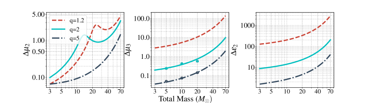
Figure 1: Projected $1\sigma$ errors on $\mu_{2}$, $\mu_{3}$ and $\epsilon_{2}$ as a functions of the total mass for the aLIGO noise PSD. Results from Bayesian analysis using MCMC sampling are given as dots showing good agreement. All the sources are considered to be at a fixed luminosity distance of 100 Mpc.

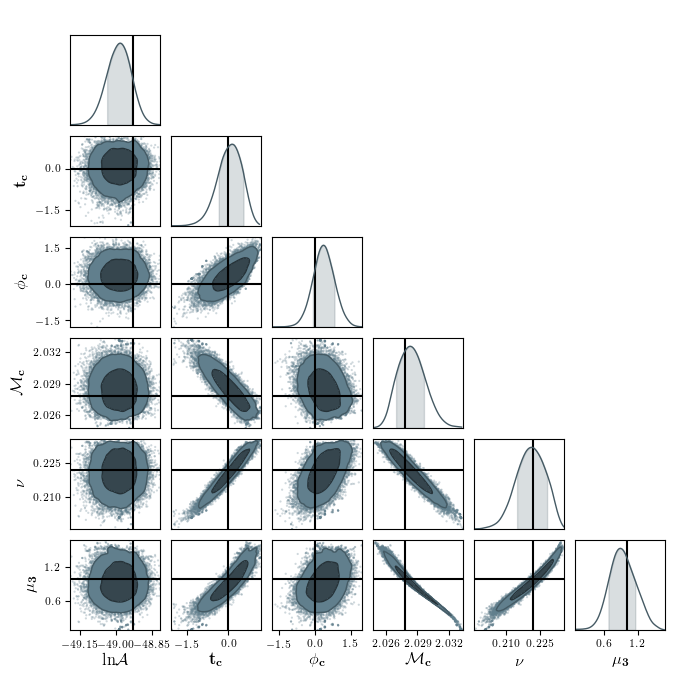
Figure 2: The posterior distributions of all six parameters $\{{\rm ln}\mathcal{A},t_{c},\phi_{c},\mathcal{M}_{c},\nu,\mu_{3}\}$ and their corresponding contour plots obtained from the MCMC experiments (see Sec. III for details) for a compact binary system at a distance of 100 Mpc with $q=2$, $m=5\text{ M}_{\odot}$ using the noise PSD of aLIGO. The darker shaded regions in the posterior distributions as well as in the contour plots shows the $1\sigma$ bounds on the respective parameters.

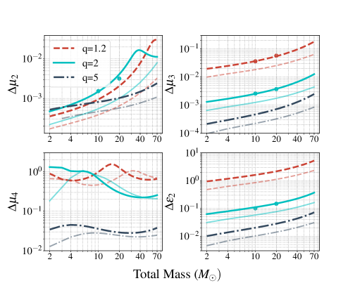
Figure 3: Dark shaded curves correspond to the projected $1\sigma$ error bars on $\mu_{2}$, $\mu_{3}$, $\mu_{4}$ and $\epsilon_{2}$ using the proposed CE-wb noise PSD as a function of the total mass, where as lighter shades denote the bounds obtained using the ET-D noise PSD. All the sources are considered to be at a fixed luminosity distance of 100 Mpc. The higher-order multipole moments such as $\mu_{4}$ and $\epsilon_{2}$ cannot be measured well using aLIGO and hence it may be a unique science goal of the third-generation detectors.

Figure 4: The posterior distributions of all six parameters $\{{\rm ln}\mathcal{A},t_{c},\phi_{c},\mathcal{M}_{c},\nu,\mu_{3}\}$ and their corresponding contour plots obtained from the MCMC experiments (see Sec. III for details) for a compact binary system at a distance of 100 Mpc with $q=2$, $m=10\text{ M}_{\odot}$ using the noise PSD of CE-wb. The darker shaded region in the posterior distributions as well as in the contour plots shows the $1\sigma$ bounds on the respective parameters.

All of the parameter estimations for aLIGO, CE-wb and LISA, that we carry out here, assume detections of the signals with a single detector, whereas for ET-D, due to its triangular shape, we consider the noise PSD to be enhanced roughly by a factor of 1.5. As our aim is to estimate the intrinsic parameters of the signal, which directly affect the binary dynamics, the single detector estimates are good enough for our purposes and a network of detectors may improve it by the square root of the number of detectors. Hence the reported errors are likely to give rough, but conservative, estimates of the expected accuracies with which the multipole coefficients may be estimated.

IV Results and Discussion

In this section, we report the $1\sigma$ measurement errors on the multipole coefficients introduced in the previous section, obtained using the Fisher matrix as well as Bayesian analysis and discuss their implications.

Our results for the four different detector configurations are presented in Figs. 1,  3 and 5 which show the errors on the various multipole coefficients ${\mu_{l}},{\epsilon_{l}}$ for aLIGO, ET-D, CE-wb and LISA, respectively. For all of these estimates we consider the sources at fixed distances. In addition to the intrinsic parameters there are four more (angular) parameters that are needed to completely specify the gravitational waveform. More specifically one needs two angles to define the location of the source on the sky and another two angles to specify the orientation of the orbital plane with respect to the detector plane Sathyaprakash and Schutz (2009). Since we are using a pattern-averaged waveform Damour et al. (2000) (i.e., a waveform averaged over all four angles), the luminosity distance can be thought of as an effective distance which we assume to be 100 Mpc for aLIGO, ET-D and CE-wb, and 3 Gpc for LISA. For aLIGO, ET-D and CE-wb, we explore the bounds for the binaries with a total mass in the range [1,70] $\text{M}_{\odot}$ and for LISA detections in the range $[10^{5},10^{7}]$ $\text{M}_{\odot}$.

IV.1 Advanced LIGO

In Fig. 1 we show the projected $1$-$\sigma$ errors on the three leading-order multipole moments, $\mu_{2},\mu_{3}$ and $\epsilon_{2},$ as a function of the total mass of the binary for the aLIGO noise PSD using the Fisher matrix. Different curves are for different mass ratios, $q=m_{1}/m_{2}=1.2$ (red), $2$ (cyan) and $5$ (blue). For the multipole coefficients considered, low-mass systems obtain the smallest errors and hence the tightest constraints. This is expected as low-mass systems live longer in the detector band and have larger number of cycles, thereby allowing us to measure the parameters very well. The bounds on $\mu_{3}$ and $\epsilon_{2}$, associated with the mass octupole and current quadrupole, increase monotonically with the total mass of the system for a given mass ratio. However, the bounds on $\mu_{2}$ show a local minimum in the intermediate-mass regime for smaller mass ratios. This is because, unlike other multipole parameters, $\mu_{2}$ appears both in the amplitude and the phase of the signal. The derivative of the waveform with respect to $\mu_{2}$ has contributions from both the amplitude and phase. Schematically, the Fisher matrix element is given by

$$\Gamma_{\mu_{2}\mu_{2}}\sim\int_{f_{\rm low}}^{f_{\rm high}}\frac{{\cal A}^{2}f^{-7/3}}{S_{h}(f)}\left(1+\mu_{2}^{2}\psi^{\prime 2}\right)\,df,$$ (25)

where $\psi^{\prime}=\partial\psi/\partial\mu_{2}$. As the inverse of this term dominantly determines the error on $\mu_{2}$, the local minimum is a result of the trade-off between the contributions from the amplitude and the phase of the waveform. Interestingly, as we go to higher mass ratios, this feature disappears resulting in a monotonically increasing curve (such as for $q=5$).

We find that the mass multipole moments $\mu_{2}$ and $\mu_{3}$ are much better estimated as compared to the current multipole moment $\epsilon_{2}$. Another important feature is that the bounds $\mu_{3}$ and $\epsilon_{2}$ are worse for equal-mass binaries. The mass-octupole and current-quadrupole are odd-parity multipole moments (unlike, say, the mass quadrupole which is even). Every odd-parity multipole moment comes with a mass asymmetry factor $\sqrt{1-4\nu}$ that vanishes in the equal-mass limit, and hence the errors diverge. Consequently, the Fisher matrix becomes badly conditioned and the precision with which we recover these parameters appears to become very poor, but this is an artifact of the Fisher matrix.

In order to cross-check the validity of the Fisher-matrix-based estimates, we performed a Bayesian analysis to find the posterior distribution of the three multipole parameters, for the same systems as in the Fisher matrix analysis. Moreover we considered a flat prior probability distribution for all six parameters $\{{\rm ln}\mathcal{A},M_{c},\nu,t_{c},\phi_{c},\mu_{\ell}\text{ or }\epsilon_{\ell}\}$ in a large enough range around their respective injection values. Given the large number of iterations, once the MCMC chains are stabilized, we find good agreements with the Fisher estimates as in the case of $\mu_{3}$ for $q=2$ and $5$, shown in Fig. 1. As an example, we present our results from the MCMC analysis for $\mu_{3}$ with $m=5\text{ M}_{\odot}$ and $q=2$, in the corner plots in Fig. 2. In Fig. 1 we see that the $1\sigma$ errors in $\mu_{3}$ from the Fisher analysis agree very well with the MCMC results for $q=2$ and $5.$ We did not find such an agreement for $q=1.2$. We suspect that this is because for comparable-mass systems the likelihood function, defined in Eq. (22), becomes shallow and it is computationally very difficult to find its maximum given a finite number of iterations. As a result, the MCMC chains did not converge and $1\sigma$ bounds cannot be trusted for such cases. We find the nonconvergence of MCMC chains for all of the cases of $\mu_{2}$ and $\epsilon_{2}$ and hence we do not show those results in Fig. 1. To summarize, our findings indicate that one can only measure $\mu_{2}$ and $\mu_{3}$ with a good enough accuracy using aLIGO detectors.

IV.2 Third-generation detectors

Third-generation detectors such as CE-wb (and ET-D) can place much better bounds on $\mu_{2},\mu_{3}$ and $\epsilon_{2}$ compared to aLIGO. Additionally, they can also measure $\mu_{4}$ with reasonable accuracy, as shown by the darker (and lighter) shaded curves in Fig. 3. The bounds on $\mu_{2}$, $\mu_{3}$ and $\epsilon_{2}$ show similar trends as in the case of aLIGO except the accuracy of the parameter estimation is much better overall. For a few cases in low-mass regime, $\mu_{2}$ and $\mu_{4}$ are better estimated for comparable-mass binaries (i.e., $q=1.2$). We also find that the bounds (represented by the lighter shaded curves in Fig. 3) obtained by using the ET-D noise PSD are even better than the bounds from CE-wb, though the other features are more or less similar for both of the detectors. This improvement in the precision of measurements is due to two reasons. The triangular shape of ET-D enhances the sensitivity roughly by a factor of 1.5 and its sensitivity is much better than CE-wb in the low-frequency region.

For a few representative cases, we compute the errors in $\mu_{2}$, $\epsilon_{2}$ and $\mu_{3}$ using Bayesian analysis and the results are shown as dots with the same color in Fig. 3. The MCMC results are in good agreement with the Fisher matrix results. Unlike the aLIGO PSD, for CE-wb the MCMC chains converge quickly in the case of $\mu_{2}$ and $\epsilon_{2}$ because of the high signal-to-noise-ratios, which naturally lead to high likelihood values. As a result, it becomes relatively easier for the sampler to find the global maximum of the likelihood function in relatively fewer iterations. We also show an example corner plot for the CE-wb PSD with $q=2$, $m=10\text{ M}_{\odot}$ in Fig. 4.

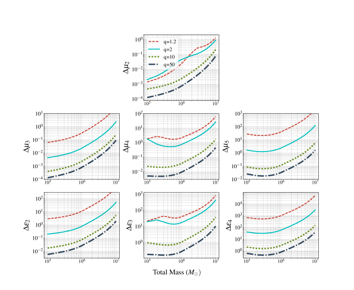
Figure 5: Projected constraints on various multipole coefficients using LISA sensitivity, as a function of the total mass of the binary. All the sources are considered to be at a fixed luminosity distance of 3 Gpc. LISA can measure all seven multipoles which contribute to the phasing and hence will be able to place extremely stringent bounds on the multipoles of the compact binary gravitational field.

IV.3 Laser Interferometer Space Antenna

In this section, we discuss the projected errors on various multipole coefficients for the LISA detector. Here we consider four different mass ratios, $q=1.2$ (red), $2$ (cyan), $10$ (blue) and $50$ (green). The first three are representatives of comparable-mass systems, while $q=50$ refers to the intermediate-mass ratio systems. We do not consider here the extreme-mass-ratio-systems, the analysis of these systems needs phasing information at much higher PN orders such as in Ref. Fujita (2012) which is beyond the scope of the present work. Moreover, in such systems, the motion of the smaller BH around the central compact object is expected to help us understand the multipolar structure of the central object and test its BH nature Ryan (1997). This is quite different from our objective here which is to use GW observations to understand the multipole structure of the gravitational field of the two-body problem in GR. The $q=50$ case, in fact, falls in between these two classes and hence has a cleaner interpretation in our framework.

In Fig. 5 we show the projected bounds from the observations of supermassive BH mergers detectable by the space-based LISA observatory. The error estimates for multipole moments with LISA are similar to that of CE-wb for mass ratios $q=1.2$, $2$. For $q=10$ all the parameters except $\epsilon_{4}$ are estimated very well. For $q=50$, we find that LISA will be able to measure all seven multipole coefficients with good accuracy. It is not entirely clear whether PN model is accurate enough for the detection and parameter estimation of supermassive binary BHs with $q=50$, for which the number of GW cycles could be an order of magnitude higher than it is for equal-mass configurations. However our findings carry important as they point to the huge potential such systems have for fundamental physics.

To summarize, we find, in general, that even-parity multipoles (i.e., $\mu_{2}$ and $\mu_{4}$) are better measured when the binary constituents are of equal or comparable masses, whereas the odd multipoles (i.e., $\mu_{3}$, $\mu_{5}$, $\epsilon_{2}$ and $\epsilon_{3}$) are better measured when the binary has mass asymmetry. This is because the even multipoles are proportional to the symmetric mass ratio $\nu,$ whereas the odd ones are proportional to the mass asymmetry $\sqrt{1-4\nu},$ which identically vanishes for equal-mass systems [see, e.g., Eq. (4.4) of Ref. Blanchet et al. (1995a)].

V Summary and Future directions

We have proposed a novel way to test for possible deviations from GR using GW observations from compact binaries by probing the multipolar structure of the GW phasing in any alternative theories of gravity. We compute a parametrized multipolar GW phasing formula that can be used to probe potential deviations from the multipolar structure of GR. Using the Fisher information matrix and Bayesian parameter estimation, we predict the accuracies with which the multipole coefficients could be measured from GW observations with present and future detectors. We find that the space mission LISA, currently under development, can measure all the multipoles of the compact binary system. Hence this will be among the unique fundamental science goals LISA can achieve.

In deriving the parametrized multipolar phasing formula, we have assumed that the conservative dynamics of the binary follow the predictions of GR. In the Appendix, we provide a phasing formula where we also deform the PN terms in the orbital energy of the binary. This should be seen as a first step towards a more complete parametrized phasing where we separate the conservative and dissipative contributions to the phasing. A systematic revisit of the problem starting from the foundations of PN theory as applied to the compact binary is needed to obtain a complete phasing formula parametrizing uniquely the conservative and dissipative sectors in the phasing formula. We postpone this for a follow up work.

The present results using nonspinning waveforms should be considered to be a proof-of-principle demonstration, to be followed up with a more realistic waveform that accounts for spin effects, effects of orbital eccentricity and higher modes. The incorporation of the proposed test in the framework of the effective one-body formalism Buonanno and Damour (1999) is also among the future directions we plan to pursue. There are ongoing efforts to implement this method in the framework of LALInference Veitch et al. (2015) so that it can be applied to the compact binaries detected by advanced LIGO and Virgo detectors.

Appendix A Frequency-domain phasing formula allowing for the deformation of conservative dynamics

The binding energy parametrized at each PN order by four different constants $\{\alpha_{0},\alpha_{1},\alpha_{2},\alpha_{3}\}$ used in the computation of parametrized GW phasing considering deviations in the conserved energy (mentioned in Sec. II.2), is given by

$$E(v) = -\frac{1}{2}\nu v^{2}\left[\alpha_{0}-\left(\frac{3}{4}+\frac{1}{12}\nu\right)\alpha_{1}v^{2}-\left(\frac{27}{8}-\frac{19}{8}\nu+\frac{1}{24}\nu^{2}\right)\alpha_{2}v^{4}\right.$$ (26)

$$\left.-\left\{\frac{675}{64}-\left(\frac{34445}{576}-\frac{205}{96}\pi^{2}\right)\nu+\frac{155}{96}\nu^{2}\right.\right.$$

$$\left.\left.+\frac{35}{5184}\nu^{3}\right\}\alpha_{3}v^{6}\right]\,.$$

The resulting phase is quoted below,

$$\psi(f) = 2\pi ft_{c}-\frac{\pi}{4}-\phi_{c}+\frac{3\alpha_{0}}{128v^{5}\mu_{2}^{2}\nu}\Bigg{\{}1+v^{2}\Bigg{(}\frac{2140}{189}-\frac{1100}{189}\nu-\frac{\alpha_{1}}{\alpha_{0}}\Bigg{[}\frac{10}{3}+\frac{10}{27}\nu\Bigg{]}+\hat{\mu}_{3}^{2}\Bigg{[}-\frac{6835}{2268}+\frac{6835}{567}\nu\Bigg{]}+\hat{\epsilon_{2}}^{2}\Bigg{[}-\frac{5}{81}+\frac{20}{81}\nu\Bigg{]}\Bigg{)}$$ (27)

$$-16\pi v^{3}+v^{4}\Bigg{(}\frac{295630}{1323}-\frac{267745}{2646}\nu+\frac{32240}{1323}\nu^{2}+\frac{\alpha_{1}}{\alpha_{0}}\Bigg{[}-\frac{535}{7}+\frac{1940}{63}\nu+\frac{275}{63}\nu^{2}\Bigg{]}+\frac{\alpha_{2}}{\alpha_{0}}\Bigg{[}-\frac{405}{4}+\frac{285}{4}\nu-\frac{5}{4}\nu^{2}\Bigg{]}$$

$$+{\hat{\mu}_{3}}^{2}\Bigg{[}-\frac{104815}{3528}+\frac{8545}{63}\nu-\frac{29630}{441}\nu^{2}+\frac{\alpha_{1}}{\alpha_{0}}\Bigg{(}\frac{6835}{336}-\frac{34175}{432}\nu-\frac{6835}{756}\nu^{2}\Bigg{)}\Bigg{]}+{\hat{\mu}_{3}}^{2}\hat{\epsilon_{2}}^{2}\Bigg{[}\frac{6835}{9072}-\frac{6835}{1134}\nu+\frac{6835\nu^{2}}{567}\Bigg{]}$$

$$+\hat{\mu}_{3}^{4}\Bigg{[}\frac{9343445}{508032}-\frac{9343445}{63504}\nu+\frac{9343445}{31752}\nu^{2}\Bigg{]}+\hat{\mu}_{4}^{2}\Bigg{[}-\frac{89650}{3969}+\frac{179300}{1323}\nu-\frac{89650}{441}\nu^{2}\Bigg{]}+\hat{\epsilon_{2}}^{2}\Bigg{[}-\frac{1885}{756}+\frac{695}{63}\nu$$

$$-\frac{800}{189}\nu^{2}+\frac{\alpha_{1}}{\alpha_{0}}\Bigg{(}\frac{5}{12}-\frac{175}{108}\nu-\frac{5}{27}\nu^{2}\Bigg{)}\Bigg{]}+\hat{\epsilon_{2}}^{4}\Bigg{[}\frac{5}{648}-\frac{5}{81}\nu+\frac{10}{81}\nu^{2}\Bigg{]}+\hat{\epsilon_{3}}^{2}\Bigg{[}-\frac{50}{63}+\frac{100}{21}\nu-\frac{50}{7}\nu^{2}\Bigg{]}\Bigg{)}$$

$$+\pi v^{5}\Big{(}3\log\left[\frac{v}{v_{\rm LSO}}\right]+1\Big{)}\Bigg{(}\frac{80}{189}\Big{[}214-131\nu\Big{]}-\frac{80\alpha_{1}}{27\alpha_{0}}\Big{[}9+\nu\Big{]}-\frac{9115}{756}\hat{\mu}_{3}^{2}\Big{[}1-4\nu\Big{]}-\frac{20}{27}\hat{\epsilon_{2}}^{2}\Big{[}1-4\nu\Big{]}\Bigg{)}$$

$$+v^{6}\Bigg{(}\frac{36847016}{509355}-\frac{640}{3}\pi^{2}-\frac{6848}{21}\gamma_{E}-\frac{6848}{21}\log[4v]+\Bigg{[}\frac{28398155}{67914}+\frac{205}{12}\pi^{2}\Bigg{]}\nu-\frac{563225}{3773}\nu^{2}+\frac{3928700}{305613}\nu^{3}$$

$$+\frac{\alpha_{1}}{\alpha_{0}}\Bigg{[}\frac{295630}{441}-\frac{1818445}{7938}\nu+\frac{312575}{7938}\nu^{2}+\frac{32240}{3969}\nu^{3}\Bigg{]}+\frac{\alpha_{2}}{\alpha_{0}}\Bigg{[}\frac{14445}{14}-\frac{8795}{7}\nu+\frac{8105}{21}\nu^{2}-\frac{275}{42}\nu^{3}\Bigg{]}$$

$$+\frac{\alpha_{3}}{\alpha_{0}}\Bigg{[}\frac{3375}{4}+\Bigg{(}-\frac{172225}{36}+\frac{1025}{6}\pi^{2}\Bigg{)}\nu+\frac{775}{6}\nu^{2}+\frac{175}{324}\nu^{3}\Bigg{]}+\hat{\mu}_{3}^{2}\Bigg{[}\frac{732782515}{3667356}-\frac{1061322545}{1222452}\nu+\frac{1027073335}{3667356}\nu^{2}$$

$$-\frac{15723035}{916839}\nu^{3}+\frac{\alpha_{1}}{\alpha_{0}}\Bigg{(}-\frac{104815}{1176}+\frac{4201865}{10584}\nu-\frac{206855}{1323}\nu^{2}-\frac{29630}{1323}\nu^{3}\Bigg{)}+\frac{\alpha_{2}}{\alpha_{0}}\Bigg{(}-\frac{61515}{224}+\frac{868045}{672}\nu-\frac{1565215}{2016}\nu^{2}$$

$$+\frac{6835}{504}\nu^{3}\Bigg{)}\Bigg{]}+\hat{\mu}_{3}^{2}\hat{\epsilon_{2}}^{2}\Bigg{[}-\frac{1742995}{190512}+\frac{1045805}{13608}\nu-\frac{2091650}{11907}\nu^{2}+\frac{697310}{11907}\nu^{3}+\frac{\alpha_{1}}{\alpha_{0}}\Bigg{(}\frac{6835}{3024}-\frac{485285}{27216}\nu+\frac{116195}{3402}\nu^{2}+\frac{6835}{1701}\nu^{3}\Bigg{)}\Bigg{]}$$

$$+\hat{\mu}_{3}^{2}\hat{\epsilon_{2}}^{4}\Bigg{[}\frac{6835}{108864}-\frac{6835}{9072}\nu+\frac{6835}{2268}\nu^{2}-\frac{6835}{1701}\nu^{3}\Bigg{]}+\hat{\mu}_{3}^{2}\hat{\epsilon_{3}}^{2}\Bigg{[}-\frac{34175}{7938}+\frac{170875}{3969}\nu-\frac{375925}{2646}\nu^{2}+\frac{68350}{441}\nu^{3}\Bigg{]}$$

$$+\hat{\mu}_{3}^{2}\hat{\mu}_{4}^{2}\Bigg{[}-\frac{61275775}{500094}+\frac{306378875}{250047}\nu-\frac{674033525}{166698}\nu^{2}+\frac{122551550}{27783}\nu^{3}\Bigg{]}+\hat{\mu}_{3}^{4}\Bigg{[}\frac{140055985}{5334336}-\frac{1148286835}{5334336}\nu+\frac{307950925}{666792}\nu^{2}$$

$$-\frac{27838955}{333396}\nu^{3}+\frac{\alpha_{1}}{\alpha_{0}}\Bigg{(}\frac{9343445}{169344}-\frac{663384595}{1524096}\nu+\frac{158838565}{190512}\nu^{2}+\frac{9343445}{95256}\nu^{3}\Bigg{)}\Bigg{]}+\hat{\mu}_{3}^{4}\hat{\epsilon_{2}}^{2}\Bigg{[}\frac{9343445}{3048192}-\frac{9343445}{254016}\nu$$

$$+\frac{9343445}{63504}\nu^{2}-\frac{9343445}{47628}\nu^{3}\Bigg{]}+\hat{\mu}_{3}^{6}\Bigg{[}\frac{12772489315}{256048128}-\frac{12772489315}{21337344}\nu+\frac{12772489315}{5334336}\nu^{2}-\frac{12772489315}{4000752}\nu^{3}\Bigg{]}$$

$$+\hat{\mu}_{4}^{2}\Bigg{[}-\frac{24426860}{916839}+\frac{62508560}{305613}\nu-\frac{12980600}{33957}\nu^{2}+\frac{286700}{11319}\nu^{3}+\frac{\alpha_{1}}{\alpha_{0}}\Bigg{(}-\frac{89650}{1323}+\frac{4751450}{11907}\nu-\frac{2241250}{3969}\nu^{2}-\frac{89650}{1323}\nu^{3}\Bigg{)}\Bigg{]}$$

$$+\hat{\mu}_{4}^{2}\hat{\epsilon_{2}}^{2}\Bigg{[}-\frac{89650}{35721}+\frac{896500}{35721}\nu-\frac{986150}{11907}\nu^{2}+\frac{358600\nu^{3}}{3969}\Bigg{]}+\hat{\mu}_{5}^{2}\Bigg{[}\frac{1002569}{12474}-\frac{4010276}{6237}\nu+\frac{10025690}{6237}\nu^{2}-\frac{8020552}{6237}\nu^{3}\Bigg{]}$$

$$+\hat{\epsilon_{2}}^{2}\Bigg{[}\frac{6134935}{190512}-\frac{2353285}{15876}\nu+\frac{550075}{6804}\nu^{2}-\frac{150845}{11907}\nu^{3}+\frac{\alpha_{1}}{\alpha_{0}}\Bigg{(}-\frac{1885}{252}+\frac{73175}{2268}\nu-\frac{1705}{189}\nu^{2}-\frac{800}{567}\nu^{3}\Bigg{)}$$

$$+\frac{\alpha_{2}}{\alpha_{0}}\Bigg{(}-\frac{45}{8}+\frac{635}{24}\nu-\frac{1145}{72}\nu^{2}+\frac{5}{18}\nu^{3}\Bigg{)}\Bigg{]}+\hat{\epsilon_{2}}^{2}\hat{\epsilon_{3}}^{2}\Bigg{[}-\frac{50}{567}+\frac{500}{567}\nu-\frac{550}{189}\nu^{2}+\frac{200}{63}\nu^{3}\Bigg{]}+\hat{\epsilon_{2}}^{4}\Bigg{[}-\frac{25}{126}+\frac{3775}{2268}\nu-\frac{2150}{567}\nu^{2}$$

$$+\frac{100}{81}\nu^{3}+\frac{\alpha_{1}}{\alpha_{0}}\Bigg{(}\frac{5}{216}-\frac{355}{1944}\nu+\frac{85}{243}\nu^{2}+\frac{10}{243}\nu^{3}\Bigg{)}\Bigg{]}+\hat{\epsilon_{2}}^{6}\Bigg{[}\frac{5}{11664}-\frac{5}{972}\nu+\frac{5}{243}\nu^{2}-\frac{20}{729}\nu^{3}\Bigg{]}+\hat{\epsilon_{3}}^{2}\Bigg{[}\frac{37180}{3969}-\frac{235640}{3969}\nu$$

$$+\frac{420200}{3969}\nu^{2}-\frac{47900}{1323}\nu^{3}+\frac{\alpha_{1}}{\alpha_{0}}\Bigg{(}-\frac{50}{21}+\frac{2650}{189}\nu-\frac{1250}{63}\nu^{2}-\frac{50}{21}\nu^{3}\Bigg{)}\Bigg{]}+\hat{\epsilon_{4}}^{2}\Bigg{[}\frac{5741}{1764}-\frac{11482}{441}\nu+\frac{28705}{441}\nu^{2}-\frac{22964}{441}\nu^{3}\Bigg{]}\Bigg{)}$$

$$+\pi v^{7}\Bigg{(}\frac{2365040}{1323}-\frac{1300930}{1323}\nu+\frac{400930}{1323}\nu^{2}+\frac{\alpha_{1}}{\alpha_{0}}\Bigg{[}-\frac{4280}{7}+\frac{19300}{63}\nu+\frac{2620}{63}\nu^{2}\Bigg{]}+\frac{\alpha_{2}}{\alpha_{0}}\Big{(}-810+570\nu-10\nu^{2}\Big{)}$$

$$+\hat{\mu}_{3}^{2}\Bigg{[}-\frac{69905}{588}+\frac{191495}{336}\nu-\frac{73995}{196}\nu^{2}+\frac{\alpha_{1}}{\alpha_{0}}\Bigg{(}\frac{9115}{112}-\frac{45575}{144}\nu-\frac{9115}{252}\nu^{2}\Bigg{)}\Bigg{]}+\hat{\mu}_{3}^{2}\hat{\epsilon_{2}}^{2}\Bigg{[}\frac{54685}{9072}-\frac{54685}{1134}\nu+\frac{54685}{567}\nu^{2}\Bigg{]}$$

$$+\hat{\mu}_{3}^{4}\Bigg{[}\frac{6835}{254016}-\frac{6835}{31752}\nu+\frac{6835}{15876}\nu^{2}\Bigg{]}+\hat{\mu}_{4}^{2}\Bigg{[}-\frac{400}{3969}+\frac{800}{1323}\nu-\frac{400}{441}\nu^{2}\Bigg{]}+\hat{\epsilon_{2}}^{2}\Bigg{[}-\frac{1885}{63}+\frac{2815}{21}\nu-\frac{3620}{63}\nu^{2}$$

$$+\frac{\alpha_{1}}{\alpha_{0}}\Bigg{(}5-\frac{175}{9}\nu-\frac{20}{9}\nu^{2}\Bigg{)}\Bigg{]}+\hat{\epsilon_{3}}^{2}\Bigg{[}-\frac{400}{63}+\frac{800}{21}\nu-\frac{400}{7}\nu^{2}\Bigg{]}+\hat{\epsilon_{2}}^{4}\Bigg{[}\frac{10}{81}-\frac{80}{81}\nu+\frac{160}{81}\nu^{2}\Bigg{]}\Bigg{)}\Bigg{\}}\,.$$

The GW phasing for compact binaries can be represented by various PN approximants depending on the different ways in which they treat the energy and flux functions. We refer the reader to Refs. Damour et al. (2002); Buonanno et al. (2009) for a detailed discussion of these various approximants. We provide the input functions required for the computation of the phasing for TaylorT2, TaylorT3 and TaylorT4 in a Mathematica file (supl-Multipole.m) which serves the Supplemental Material to this paper. We closely follow the notations of Ref. Buonanno et al. (2009) in this file.

References

- Abbott et al. (2016a) B. P. Abbott et al. (Virgo, LIGO Scientific), Phys. Rev. Lett. 116, 061102 (2016a), eprint 1602.03837.
- Abbott et al. (2016b) B. P. Abbott et al. (Virgo, LIGO Scientific), Phys. Rev. Lett. 116, 241103 (2016b), eprint 1606.04855.
- Abbott et al. (2017a) B. P. Abbott et al., Phys. Rev. Lett. 118, 221101 (2017a), eprint 1706.01812.
- Abbott et al. (2017b) B. P. Abbott et al. (Virgo, LIGO Scientific), Phys. Rev. Lett. 119, 141101 (2017b), eprint 1709.09660.
- Abbott et al. (2017c) B. Abbott et al., Phys. Rev. Lett. 119, 161101 (2017c), eprint 1710.05832.
- Collaboration et al. (2015) T. L. S. Collaboration, J. Aasi, B. P. Abbott, R. Abbott, T. Abbott, M. R. Abernathy, K. Ackley, C. Adams, T. Adams, P. Addesso, et al., Classical and Quantum Gravity 32, 074001 (2015).
- Acernese et al. (2015) F. Acernese, M. Agathos, K. Agatsuma, D. Aisa, N. Allemandou, A. Allocca, J. Amarni, P. Astone, G. Balestri, G. Ballardin, et al., Classical and Quantum Gravity 32, 024001 (2015).
- Sathyaprakash and Schutz (2009) B. Sathyaprakash and B. Schutz, Living Rev.Rel. 12, 2 (2009), eprint arXiv:0903.0338.
- Yunes and Siemens (2013) N. Yunes and X. Siemens, Living Rev. Rel. 16, 9 (2013), eprint 1304.3473.
- Abbott et al. (2016c) B. P. Abbott et al. (Virgo, LIGO Scientific), Phys. Rev. Lett. 116, 221101 (2016c), eprint 1602.03841.
- Abbott et al. (2016d) B. P. Abbott et al. (Virgo, LIGO Scientific), Phys. Rev. X6, 041015 (2016d), eprint 1606.04856.
- Arun et al. (2006a) K. G. Arun, B. R. Iyer, M. S. S. Qusailah, and B. S. Sathyaprakash, Class. Quantum Grav. 23, L37 (2006a), eprint gr-qc/0604018.
- Arun et al. (2006b) K. G. Arun, B. R. Iyer, M. S. S. Qusailah, and B. S. Sathyaprakash, Phys. Rev. D 74, 024006 (2006b), eprint gr-qc/0604067.
- Yunes and Pretorius (2009) N. Yunes and F. Pretorius, Phys. Rev. D 80, 122003 (2009), eprint 0909.3328.
- Mishra et al. (2010) C. K. Mishra, K. G. Arun, B. R. Iyer, and B. S. Sathyaprakash, Phys. Rev. D 82, 064010 (2010), eprint 1005.0304.
- Agathos et al. (2014) M. Agathos, W. Del Pozzo, T. G. F. Li, C. V. D. Broeck, J. Veitch, et al., Phys.Rev. D89, 082001 (2014), eprint 1311.0420.
- Li et al. (2012) T. G. F. Li, W. Del Pozzo, S. Vitale, C. Van Den Broeck, M. Agathos, J. Veitch, K. Grover, T. Sidery, R. Sturani, and A. Vecchio, Phys. Rev. D85, 082003 (2012), eprint 1110.0530.
- Meidam et al. (2018) J. Meidam et al., Phys. Rev. D97, 044033 (2018), eprint 1712.08772.
- Will (1998) C. M. Will, Phys. Rev. D 57, 2061 (1998), eprint gr-qc/9709011.
- Mirshekari et al. (2012) S. Mirshekari, N. Yunes, and C. M. Will, Phys. Rev. D 85, 024041 (2012), eprint 1110.2720.
- Ghosh et al. (2016) A. Ghosh et al., Phys. Rev. D94, 021101 (2016), eprint 1602.02453.
- Abbott et al. (2017d) B. P. Abbott et al. (Virgo, Fermi-GBM, INTEGRAL, LIGO Scientific), Astrophys. J. 848, L13 (2017d), eprint 1710.05834.
- Yunes et al. (2016) N. Yunes, K. Yagi, and F. Pretorius, Phys. Rev. D94, 084002 (2016), eprint 1603.08955.
- Abernathy et al. (2010) M. Abernathy et al., Einstein gravitational wave Telescope: Conceptual Design Study (Document number ET-0106A-10) (2010), eprint ET-0106A-10.
- Abbott et al. (2017e) B. P. Abbott et al. (LIGO Scientific), Class. Quant. Grav. 34, 044001 (2017e), eprint 1607.08697.
- (26) https://lisa.nasa.gov/.
- Miller and Colbert (2004) M. C. Miller and E. J. M. Colbert, Int. J. Mod. Phys. D13, 1 (2004), eprint astro-ph/0308402.
- van der Marel (2003) R. P. van der Marel, in Carnegie Observatories Centennial Symposium. 1. Coevolution of Black Holes and Galaxies Pasadena, California, October 20-25, 2002 (2003), eprint astro-ph/0302101.
- Fregeau et al. (2006) J. M. Fregeau, S. L. Larson, M. C. Miller, R. W. O’Shaughnessy, and F. A. Rasio, Astrophys. J. 646, L135 (2006), eprint astro-ph/0605732.
- Graff et al. (2015) P. B. Graff, A. Buonanno, and B. S. Sathyaprakash, Phys. Rev. D92, 022002 (2015), eprint 1504.04766.
- Brown et al. (2007) D. A. Brown, H. Fang, J. R. Gair, C. Li, G. Lovelace, I. Mandel, and K. S. Thorne, Phys. Rev. Lett. 99, 201102 (2007), eprint gr-qc/0612060.
- Chamberlain and Yunes (2017) K. Chamberlain and N. Yunes, Phys. Rev. D96, 084039 (2017), eprint 1704.08268.
- Ryan (1997) F. Ryan, Phys. Rev. D 56, 1845 (1997).
- Thorne (1995) K. S. Thorne, in Particle and nuclear astrophysics and cosmology in the next millennium. Proceedings, Summer Study, Snowmass, USA, June 29-July 14, 1994 (1995), pp. 0160–184, eprint gr-qc/9506086.
- Schutz (1996) B. F. Schutz, Classical and Quantum Gravity 13, A219 (1996).
- Gair et al. (2013) J. R. Gair, M. Vallisneri, S. L. Larson, and J. G. Baker, Living Rev. Rel. 16, 7 (2013), eprint 1212.5575.
- Berti et al. (2015) E. Berti, E. Barausse, V. Cardoso, L. Gualtieri, P. Pani, U. Sperhake, L. C. Stein, N. Wex, K. Yagi, T. Baker, et al., Classical and Quantum Gravity 32, 243001 (2015), eprint 1501.07274.
- Arun and Pai (2013) K. G. Arun and A. Pai, Int.J.Mod.Phys. D 22, 1341012 (2013), eprint 1302.2198.
- Giudice et al. (2016) G. F. Giudice, M. McCullough, and A. Urbano, JCAP 1610, 001 (2016), eprint 1605.01209.
- Chirenti and Rezzolla (2016) C. Chirenti and L. Rezzolla, Phys. Rev. D94, 084016 (2016), eprint 1602.08759.
- Cardoso et al. (2016) V. Cardoso, E. Franzin, and P. Pani, Phys. Rev. Lett. 116, 171101 (2016), eprint 1602.07309.
- Cardoso et al. (2017) V. Cardoso, E. Franzin, A. Maselli, P. Pani, and G. Raposo, Phys. Rev. D95, 084014 (2017), [Addendum: Phys. Rev.D95,no.8,089901(2017)], eprint 1701.01116.
- Johnson-Mcdaniel et al. (2018) N. K. Johnson-Mcdaniel, A. Mukherjee, R. Kashyap, P. Ajith, W. Del Pozzo, and S. Vitale (2018), eprint 1804.08026.
- Krishnendu et al. (2017) N. V. Krishnendu, K. G. Arun, and C. K. Mishra, Phys. Rev. Lett. 119, 091101 (2017), eprint 1701.06318.
- Dhanpal et al. (2018) S. Dhanpal, A. Ghosh, A. K. Mehta, P. Ajith, and B. S. Sathyaprakash (2018), eprint 1804.03297.
- Krishnendu et al. (2018) N. V. Krishnendu, C. K. Mishra, and K. G. Arun (2018), eprint 1811.00317.
- Blanchet (2014) L. Blanchet, Living Rev. Rel. 17, 2 (2014), eprint 1310.1528.
- Pretorius (2007) F. Pretorius (2007), relativistic Objects in Compact Binaries: From Birth to Coalescence, Editor=Colpi et al., eprint arXiv:0710.1338.
- Sasaki and Tagoshi (2003) M. Sasaki and H. Tagoshi, Living Rev. Rel. 6, 6 (2003), eprint gr-qc/0306120.
- Blanchet and Sathyaprakash (1994) L. Blanchet and B. S. Sathyaprakash, Class. Quantum Grav. 11, 2807 (1994).
- Blanchet and Sathyaprakash (1995) L. Blanchet and B. S. Sathyaprakash, Phys. Rev. Lett. 74, 1067 (1995).
- Blanchet et al. (1995a) L. Blanchet, T. Damour, and B. R. Iyer, Phys. Rev. D 51, 5360 (1995a), eprint gr-qc/9501029.
- Endlich et al. (2017) S. Endlich, V. Gorbenko, J. Huang, and L. Senatore, JHEP 09, 122 (2017), eprint 1704.01590.
- Rao (1945) C. Rao, Bullet. Calcutta Math. Soc 37, 81 (1945).
- Cramer (1946) H. Cramer, Mathematical methods in statistics (Pergamon Press, Princeton University Press, NJ, U.S.A., 1946).
- Foreman-Mackey et al. (2013) D. Foreman-Mackey, D. W. Hogg, D. Lang, and J. Goodman, Publications of the Astronomical Society of the Pacific 125, 306 (2013), eprint 1202.3665.
- Thorne (1980) K. Thorne, Rev. Mod. Phys. 52, 299 (1980).
- Blanchet and Damour (1984) L. Blanchet and T. Damour, Phys. Lett. A 104, 82 (1984).
- Blanchet and Damour (1986) L. Blanchet and T. Damour, Phil. Trans. Roy. Soc. Lond. A 320, 379 (1986).
- Blanchet (1987) L. Blanchet, Proc. Roy. Soc. Lond. A 409, 383 (1987).
- Blanchet and Damour (1988a) L. Blanchet and T. Damour, Phys. Rev. D 37, 1410 (1988a).
- Blanchet and Damour (1989) L. Blanchet and T. Damour, Annales Inst. H. Poincaré Phys. Théor. 50, 377 (1989).
- Blanchet and Damour (1992) L. Blanchet and T. Damour, Phys. Rev. D 46, 4304 (1992).
- Blanchet (1995) L. Blanchet, Phys. Rev. D 51, 2559 (1995), eprint gr-qc/9501030.
- Blanchet et al. (2002a) L. Blanchet, B. R. Iyer, and B. Joguet, Phys. Rev. D 65, 064005 (2002a), Erratum-ibid 71, 129903(E) (2005), eprint gr-qc/0105098.
- Damour et al. (2001a) T. Damour, P. Jaranowski, and G. Schäfer, Phys. Lett. B 513, 147 (2001a).
- Blanchet et al. (2004a) L. Blanchet, T. Damour, G. Esposito-Farèse, and B. R. Iyer, Phys. Rev. Lett. 93, 091101 (2004a), eprint gr-qc/0406012.
- Damour and Iyer (1991) T. Damour and B. R. Iyer, Phys. Rev. D 43, 3259 (1991).
- Blanchet and Damour (1988b) L. Blanchet and T. Damour, Phys. Rev. D37, 1410 (1988b).
- Blanchet and Schaefer (1993) L. Blanchet and G. Schaefer, Class. Quant. Grav. 10, 2699 (1993).
- Blanchet (1998a) L. Blanchet, Class. Quantum Grav. 15, 113 (1998a), eprint gr-qc/9710038.
- Blanchet (1998b) L. Blanchet, Class. Quantum Grav. 15, 89 (1998b), eprint gr-qc/9710037.
- Christodoulou (1991) D. Christodoulou, Phys. Rev. Lett. 67, 1486 (1991).
- Thorne (1992) K. Thorne, Phys. Rev. D 45, 520 (1992).
- Arun et al. (2004) K. G. Arun, L. Blanchet, B. R. Iyer, and M. S. S. Qusailah, Class. Quantum Grav. 21, 3771 (2004), erratum-ibid. 22, 3115 (2005), eprint gr-qc/0404185.
- Favata (2009) M. Favata, Phys. Rev. D 80, 024002 (2009), eprint 0812.0069.
- Blanchet et al. (1995b) L. Blanchet, T. Damour, B. R. Iyer, C. M. Will, and A. G. Wiseman, Phys. Rev. Lett. 74, 3515 (1995b), eprint gr-qc/9501027.
- Blanchet et al. (2002b) L. Blanchet, G. Faye, B. R. Iyer, and B. Joguet, Phys. Rev. D 65, 061501(R) (2002b), Erratum-ibid 71, 129902(E) (2005), eprint gr-qc/0105099.
- Blanchet and Iyer (2003) L. Blanchet and B. R. Iyer, Class. Quantum Grav. 20, 755 (2003), eprint gr-qc/0209089.
- Blanchet et al. (2004b) L. Blanchet, T. Damour, and G. Esposito-Farèse, Phys. Rev. D 69, 124007 (2004b), eprint gr-qc/0311052.
- Damour et al. (2001b) T. Damour, P. Jaranowski, and G. Schäfer, Phys. Rev. D 63, 044021 (2001b), erratum-ibid 66, 029901(E) (2002).
- de Andrade et al. (2001) V. de Andrade, L. Blanchet, and G. Faye, Class. Quantum Grav. 18, 753 (2001).
- Itoh and Futamase (2003) Y. Itoh and T. Futamase, Phys. Rev. D 68, 121501(R) (2003).
- Blanchet (1996) L. Blanchet, Phys. Rev. D 54, 1417 (1996), Erratum-ibid.71, 129904(E) (2005), eprint gr-qc/9603048.
- Iyer and Will (1993) B. R. Iyer and C. M. Will, Phys. Rev. Lett. 70, 113 (1993).
- Iyer and Will (1995) B. R. Iyer and C. M. Will, Phys. Rev. D 52, 6882 (1995).
- Damour et al. (2000) T. Damour, B. R. Iyer, and B. S. Sathyaprakash, Phys. Rev. D 62, 084036 (2000), eprint gr-qc/0001023.
- Buonanno et al. (2009) A. Buonanno, B. Iyer, E. Ochsner, Y. Pan, and B. S. Sathyaprakash, Phys. Rev. D80, 084043 (2009), eprint 0907.0700.
- Sathyaprakash and Dhurandhar (1991) B. S. Sathyaprakash and S. V. Dhurandhar, Phys. Rev. D44, 3819 (1991).
- Blanchet et al. (1996) L. Blanchet, B. R. Iyer, C. M. Will, and A. G. Wiseman, Class. Quantum Grav. 13, 575 (1996), eprint gr-qc/9602024.
- Blanchet et al. (2008) L. Blanchet, G. Faye, B. R. Iyer, and S. Sinha, Class. Quantum. Grav. 25, 165003 (2008), eprint 0802.1249.
- Cutler and Flanagan (1994) C. Cutler and E. Flanagan, Phys. Rev. D 49, 2658 (1994).
- Arun et al. (2005) K. G. Arun, B. R. Iyer, B. S. Sathyaprakash, and P. A. Sundararajan, Phys. Rev. D 71, 084008 (2005), erratum-ibid. D 72, 069903 (2005), eprint gr-qc/0411146.
- Balasubramanian et al. (1995) R. Balasubramanian, B. S. Sathyaprakash, and S. V. Dhurandhar, Pramana 45, L463 (1995), eprint gr-qc/9508025.
- Vallisneri (2008) M. Vallisneri, Phys. Rev. D 77, 042001 (2008), eprint gr-qc/0703086.
- Abbott et al. (2017f) B. Abbott, R. Abbott, T. Abbott, M. Abernathy, K. Ackley, C. Adams, P. Addesso, R. Adhikari, V. Adya, C. Affeldt, et al., Classical and Quantum Gravity 34 (2017f), ISSN 0264-9381.
- Ajith (2011) P. Ajith, Phys.Rev. D84, 084037 (2011), eprint 1107.1267.
- Babak et al. (2017) S. Babak, J. Gair, A. Sesana, E. Barausse, C. F. Sopuerta, C. P. L. Berry, E. Berti, P. Amaro-Seoane, A. Petiteau, and A. Klein, ArXiv e-prints (2017), eprint 1703.09722.
- Fujita (2012) R. Fujita, Prog. Theor. Phys. 128, 971 (2012), eprint 1211.5535.
- Buonanno and Damour (1999) A. Buonanno and T. Damour, Phys. Rev. D 59, 084006 (1999), eprint gr-qc/9811091.
- Veitch et al. (2015) J. Veitch et al., Phys. Rev. D91, 042003 (2015), eprint 1409.7215.
- Damour et al. (2002) T. Damour, B. R. Iyer, and B. S. Sathyaprakash, Phys. Rev. D 66, 027502 (2002), erratum-ibid 66, 027502 (2002), eprint gr-qc/0207021.