Evolution of two-time correlations in dissipative quantum spin systems: aging and hierarchical dynamics

Abstract

We consider the evolution of two-time correlations in the quantum XXZ spin-chain in contact with an environment causing dephasing. Extending quasi-exact time-dependent matrix product state techniques to consider the dynamics of two-time correlations within dissipative systems, we uncover the full quantum behavior for these correlations along all spin directions. Together with insights from adiabatic elimination and kinetic Monte Carlo, we identify three dynamical regimes. For initial times, their evolution is dominated by the system unitary dynamics and depends on the initial state and the Hamiltonian parameters. For weak spin-spin interaction anisotropy, after this initial dynamical regime, two-time correlations enter an algebraic scaling regime signaling the breakdown of time-translation invariance and the emergence of aging. For stronger interaction anisotropy, these correlations first go through a stretched exponential regime before entering the algebraic one. Such complex relaxation arises due to the competition between the proliferation dynamics of energetically costly excitations and their motion. As a result, dissipative heating dynamics of spin systems can be used to probe the entire spectrum of the underlying Hamiltonian.

Two-time correlations are powerful tools to capture the fundamental dynamical features of many-body systems both in and away from equilibrium. These correlation functions are of the form $\langle B(t_{2})A(t_{1})\rangle$ where $A$ and $B$ are operators, $t_{1}$ and $t_{2}$ are two different times, and $\langle\dots\rangle=\text{tr}(\rho\dots)$ is the average over the density matrix $\rho$ of a given system.

Numerous experimental techniques have been developed to probe these correlations measuring the response of many-body systems. A non-exhaustive list includes ARPES Lu et al. (2012), neutron scattering Bramwell and Keimer (2014) or conductivity and magnetization measurements in solids Ashcroft and Mermin (1976), and radio-frequency Stewart et al. (2008), Raman, Bragg Esslinger (2010) (and references therein) or modulation spectroscopy Stöferle et al. (2004) in cold gases. In equilibrium, these experimental methods provide information on various spectral features such as collective excitations and bound states. Whereas away from equilibrium, these techniques are employed to identify the formation of dynamically induced states in isolated quantum systems subjected to an external parameter change, and to capture, using for example magnetic susceptibility measurements, the aging dynamics of classical spin glasses Vincent and Dupuis (2017).

Theoretically, two-time correlations have been studied in isolated many-body quantum systems (i.e. not in contact with an environment), both in and far from equilibrium. However, for open many-body quantum systems (i.e. in contact with an environment) evaluating out-of-equilibrium two-time correlations has proven extremely challenging. Most works have instead focused on characterizing the non-equilibrium dynamics of open systems by considering the universal scaling behavior of simpler observables or the propagation of single-time correlations Marino and Silva (2012); Bernier et al. (2018), by using various approximate approaches to evaluate two-time correlations Buchhold and Diehl (2015); Marcuzzi et al. (2015); Sciolla et al. (2015); Everest et al. (2017); He et al. (2017); DenisWimberger2018 , or by considering small many-body quantum systems Wang et al. (2018).

Here, for the first time, we evaluate quasi-exactly the evolution of both the two-time correlations along the $z$-spin direction, $\langle S^{z}_{l}(t_{2})S^{z}_{l+d}(t_{1})\rangle$, and along the $\pm$-spin directions, $\langle S^{+}_{l}(t_{2})S^{-}_{l+d}(t_{1})\rangle$, in a quantum XXZ spin-$1/2$ chain in contact with a memoryless environment causing dephasing. $S^{z}_{l}$ and $S^{\pm}_{l}$ are the spin-$1/2$ operators in the $z$ and $\pm$ directions at site $l$. Previous works on this system had solely focused on the evaluation of equal-time correlations along the $\pm$-spin directions Cai and Barthel (2013) identifying an algebraic regime similar to the one found for interacting bosons in contact with a dissipative environment causing dephasing Poletti et al. (2012, 2013). Additionally, in the classical limit, for large interaction anisotropies, the $\langle S^{z}_{l}(t)S^{z}_{l}(0)\rangle$ correlations were shown to display a stretched exponential behavior Everest et al. (2017).

We developed here a variant of the quasi-exact time-dependent variational matrix product state (t-MPS) technique White (1992); Schollwöck (2011) applicable to two-time correlations. Using this novel approach, we uncover the full quantum behavior of these correlations along both the $z$ and the $\pm$-spin directions when the evolution of the spin system begins from an excited state such as the Néel $|\!\!\uparrow,\downarrow,\uparrow,\downarrow,\dots,\uparrow,\downarrow\rangle$ or the single domain wall state $|\uparrow,\dots,\uparrow,\uparrow,\downarrow,\downarrow,\dots,\downarrow\rangle$. Our analysis is carried out using an implementation of t-MPS built upon the ITensor library itensor . The density matrix operator is represented as a pure state in an enlarged Hilbert space and the evolution of the two-time correlations is implemented using an approach similar to the one used to obtain their equilibrium thermal counterparts Zwolak and Vidal (2004); Verstraete et al. (2009). Taking good quantum numbers into account Bonnes and Läuchli (2014); Bernier et al. (2018) enables us to follow the quasi-exact evolution of systems for sufficiently long times to identify three interesting dynamical regimes signaled by changes in the behavior of the two-time correlations along the $z$-spin direction.

The first regime, identified at initial times, is dominated by the system unitary dynamics. This regime depends significantly on the initial state and on the Hamiltonian parameters, and, for weak dissipation, resembles the dynamics of the isolated system. The second regime, identified both numerically and analytically, is characterized by an algebraic scaling: for distances $d\geq 1$, the normalized correlations are proportional to $\left(t_{2}/t_{1}\right)^{-3/2}$ signaling the emergence of aging dynamics with broken time-translation invariance. In this particular case, this aging regime finds its origin in the presence of underlying diffusive processes. Finally, in the third regime, correlations evolve following a stretched exponential, a behavior typically associated with glasses or systems exhibiting hierarchical separation of time-scales. This regime, which we identify for the first time over a wide range of $t_{1}$ using quasi-exact simulations, only occurs for sufficiently strong interaction anisotropies when the evolution begins from initial states with occupied energy levels well separated from others. The evolution of these two-time correlations is governed by the competition between the nucleation (or annihilation) dynamics of energetically costly excitations and their motion, two processes occurring on very different time-scales.

We interpret our quasi-exact numerical findings using adiabatic elimination and kinetic Monte Carlo from which the scaling properties can be predicted, and find the observed dynamics to closely relate to the spectrum of the spin Hamiltonian. Monitoring the dynamics of two-time correlations induced by dissipative heating thus constitutes a novel approach to characterize spin systems as it reveals features spanning the entire spectrum of the underlying Hamiltonian. Let us also mention that the two-time correlations along the $\pm$-spin direction decay exponentially and therefore exhibit a completely different behavior from which the regimes mentioned earlier cannot be inferred.

To investigate the non-equilibrium dynamics of two-time correlations in an open quantum system, we consider a spin-$1/2$ chain under the effect of local dephasing noise. In such a situation, the evolution of the density operator $\rho$ is described by the Lindblad master equation

$$\frac{\partial\rho}{\partial t} =-\frac{i}{\hbar}\left[H_{\text{XXZ}},\rho\right]+\mathcal{D}(\rho).$$ (1)

The first term on the right-hand side describes the unitary evolution due to the XXZ spin-$1/2$ Hamiltonian

$$H_{\text{XXZ}}=\sum_{j=1}^{L-1}\left[J_{x}\left(S^{x}_{j}S^{x}_{j+1}+S^{y}_{j}S^{y}_{j+1}\right)+J_{z}S^{z}_{j}S^{z}_{j+1}\right],$$

where $J_{x}$ and $J_{z}$ are the exchange couplings along the different spin directions, $S^{\alpha}_{j}$ is the $\alpha$-direction spin operator at site $j$, and $L$ is the length of the chain. The isolated XXZ spin-chain is solvable by Bethe ansatz and is known to present three distinct phases Mikeska and Kolezhuk (2004): for $-1\leq J_{z}/J_{x}\leq 1$, the easy plane anisotropic phase is gapless, while $J_{z}/J_{x}<-1$ presents a gapped ferromagnetic phase, and $J_{z}/J_{x}>1$ hosts a gapped antiferromagnetic phase. The second term on the right-hand side of Eq. (1) describes the dephasing noise in Lindblad form

$$\mathcal{D}(\rho) =\gamma\sum_{j=1}^{L}\left(S^{z}_{j}\rho S^{z}_{j}-\frac{1}{4}\rho\right),$$

where $\gamma$ is the dissipation strength. This term acts like a source of heat inducing spin fluctuations and eventually drives the system towards the infinite temperature state, the unique steady state of the model. If not stated otherwise, we consider here a system initially prepared in the Néel state and investigate its dynamics as the system is coupled to the environment and starts to undergo dephasing. We access the full quantum dynamics by extending the quasi-exact t-MPS techniques available to dissipative systems to the study of two-time correlations. To gain analytical insights into the evolution of this system, we employ adiabatic elimination, valid for times larger than $1/\gamma$, to capture the dominant dissipative dynamics in the limit where $\hbar\gamma\gg J_{z}$. We focus primarily on the two-time correlations along the $z$-spin direction given by

$$\hbar^{2}~{}C_{d}(t_{2},t_{1}) = \langle S^{z}_{\frac{L}{2}}(t_{2})S^{z}_{\frac{L}{2}+d}(t_{1})\rangle,$$

where $d$ is the distance between two spins, as they provide the most insights into the dynamical properties of the system, and we also investigate the corresponding equal-time correlations.

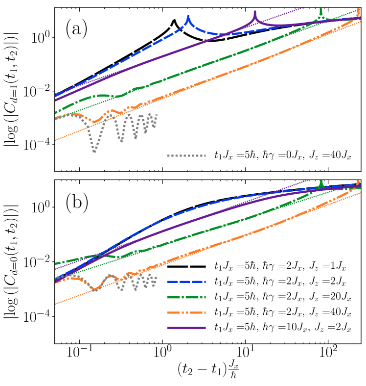
Figure 1: Initial quasi-unitary and intermediate stretched exponential regimes. Logarithm of the two-time correlation $\hbar^{2}C_{d}(t_{2},t_{1})=\langle S^{z}_{\frac{L}{2}}(t_{2})S^{z}_{\frac{L}{2}+d}(t_{1})\rangle$ for $d=1$, panel (a), and $d=0$, panel (b), versus the time difference $t_{2}-t_{1}$ (t-MPS data for $L=48$). For weak dissipation, the initial time-regime is dominated by the system unitary dynamics. The dephasing noise damps out the oscillations commonly present in the unitary evolution (dashed grey line). Following this initial regime, for sufficiently strong coupling anisotropy $J_{z}/J_{x}$, the two-time correlations follow a stretched exponential: the linear slopes indicate the presence of this regime. The thin dotted lines are fits in the linear regions.

Figure 2: Scaling regime for the two-time correlations. Panel (a): Scaling collapse for the normalized two-time correlations between neighboring sites $\hbar^{2}C_{d=1}(t_{2},t_{1})=\langle S^{z}_{\frac{L}{2}}(t_{2})S^{z}_{\frac{L}{2}+1}(t_{1})\rangle$ calculated using t-MPS for $L=80$. The black solid line is a guide to the eye and highlights the $(t_{2}/t_{1})^{-3/2}$ algebraic regime. Panel (b): Comparison between the two-time correlations obtained from t-MPS and adiabatic elimination. For large $\hbar\gamma/J_{z}$ ratios, adiabatic elimination describes two-time correlations over the whole range of $t_{2}/t_{1}$ whereas, for smaller ratios, the analytical approach successfully captures the long-time $(t_{2}/t_{1})^{-3/2}$ scaling but fails to describe the initial dynamics.

As hinted earlier, we find the normalized two-time correlations along $z$-spin direction to present three distinct dynamical regimes depending on the dissipation strength, $\hbar\gamma/J_{x}$, and the interaction anisotropy, $J_{z}/J_{x}$. For weak dissipation, the initial time-regime is governed by the system unitary dynamics. For strongly interacting systems, the dynamics is typically characterized by oscillations due to the opening of a gap in the energy spectrum. Such dynamics, illustrated by the grey dotted lines in Fig. (1), is damped by the dephasing. The other curves shown in Fig. (1) will be discussed in detail later.

After this initial unitary-like evolution, the system enters a scaling regime where the two-time correlations break time-translation invariance as they do not depend on $t_{2}-t_{1}$. This regime, which occurs at later times for stronger interaction strengths, is exemplified in Fig. (2) where the correlations for $d=1$ are shown. For $d=1$, the normalized two-time correlations scale as $\sim(t_{2}/t_{1})^{-3/2}$ and one can see that there is a regime for which curves with different $t_{1}$, $\gamma$, and $J_{z}$ nicely collapse on top of each other. As this region is characterized by the slow algebraic relaxation of correlations, and by a dynamical scaling that is solely a ratio of $t_{2}/t_{1}$, this system presents emergent aging dynamics. As for $d=0$, we find in this case that the two-time correlations also scale algebraically however they do not depend solely on a $t_{2}/t_{1}$ ratio. As explained in the Supplemental material, these scaling regimes arise when $t_{1}$ lies within an interval where the equal-time correlations along the $z$-spin direction decay algebraically.

To identify the origin of the scaling regime, we use many-body adiabatic elimination Garcia-Ripoll et al. (2009); Poletti et al. (2012) to develop a set of differential equations capturing the evolution around the dissipation-free subspace (see the Supplemental material for more details). Then, resorting to the quantum regression theorem Gardiner and Zoller (2000); Breuer and Petruccione (2002), we find the two-time correlations along the $z$-spin direction to obey the following differential equations

$$\frac{\partial}{\partial\tau}\langle S_{j}^{z}(t_{1}+\tau)S_{j+d}^{z}(t_{1})\rangle = \sum_{l}G_{j,l}\langle S_{l}^{z}(t_{1}+\tau)S_{j+d}^{z}(t_{1})\rangle$$

where $\tau=t_{2}-t_{1}$, $G_{j,l}=\frac{D}{2}(\delta_{j+1,l}+\delta_{j-1,l}-2\delta_{j,l})$, $D=\frac{J_{x}^{2}}{\hbar^{2}\gamma}$ and the initial condition, $\langle S_{j}^{z}(t_{1})S_{j+d}^{z}(t_{1})\rangle$, is the solution of the equal-time correlations at $t_{1}$ footnote1 . While these equations are in principle only valid for $J_{z}=0$ and more complicated expressions are obtained for finite $J_{z}$, we find that for sufficiently large $\hbar\gamma/J_{z}$ their solution and in particular the extracted scaling coincide well with the t-MPS results. As illustrated in Fig. (2) (b), for large $\hbar\gamma/J_{z}$, adiabatic elimination describes two-time correlations over the whole range of $t_{2}/t_{1}$, while for smaller ratios, this analytical approach describes well the long-time $(t_{2}/t_{1})^{-3/2}$ scaling but fails to capture the initial dynamics. The overall good agreement between the t-MPS simulations and the adiabatic elimination approach within the scaling regime points to the diffusive nature of the propagation of the two-time correlations under the action of dephasing. One should also note that this regime is also present if the initial state is not the Néel state but is instead made of larger domains with alternating magnetization.

Finally, the aging dynamics displayed by the correlations in the $z$-spin direction should be contrasted with the evolution of the two-time correlations along the other spin directions. For the latter, the evolution leaves the dissipation-free subspace through the application of the lowering/rising operator $S^{\pm}_{l+d}$ at $t_{1}$. As a consequence, the dissipator strongly alters the evolution and these correlations decay exponentially as a function of $t_{2}-t_{1}$: $\langle S_{i}^{+}(t_{2})S_{j}^{-}(t_{1})\rangle\propto e^{-\beta(\gamma)(t_{2}-t_{1})}$ where $\beta$ is a function of the dissipative strength $\gamma$ (see Ref. Sciolla et al. (2015)).

Another interesting regime occurs solely at larger values of the interaction anisotropy $J_{z}/J_{x}$ and for particular initial states. As shown in Fig. (1), for intermediate values of the time difference, $t_{2}-t_{1}$, we find the two-time correlations along the $z$-direction to follow a stretched exponential: $\log|C_{d}(t_{2},t_{1})|\sim(t_{2}-t_{1})^{\nu_{d}}$ where $\nu_{d}$ depends on the system parameters. We checked that this regime persists at least for distances up to $d=9$ in a system of size $L=48$. This regime originates via the occurrence of nucleation events of energetically costly excitations. For the disordered XXZ model, using classical approximations, a similar regime displaying a stretched exponential decay was previously identified for the special case of $t_{1}=0$ where the two-time correlation reduces to the single time staggered magnetization Everest et al. (2017). In comparison, here we identify, this regime for actual two-time correlation functions over a wide range of $t_{1}$ using, for the first time, quasi-exact simulations within the t-MPS formalism (see Fig. (1)). Interestingly, even for large interaction anisotropy, this stretched exponential regime gives way to the scaling regime discussed above at larger $t_{2}/t_{1}$ ratios. These two contiguous regimes are displayed in Figs. (1) and (2) for the parameters $t_{1}J_{x}=5\hbar$, $\hbar\gamma=10J_{x}$ and $J_{z}=2J_{x}$.

The mechanism behind the crossover between the stretched exponential and the algebraic regimes can be inferred by considering the proliferation of excitations caused by the dephasing noise. We expect the stretched exponential regime to be dominant only if well separated time-scales exist for the nucleation (or annihilation) of an excitation and for its motion. This separation typically occurs only for states on the lower and upper bounds of the spectrum of the XXZ model (see the well separated energy bands at the boundaries of the spectrum in the inset of Fig. (3)).

As the dissipative evolution brings the system into the infinite-temperature state, where all Hamiltonian levels are equally occupied, we expect the stretched exponential to only show up in the initial dynamics when the states at the boundaries of the spectrum are predominantly occupied. This situation explains the presence of the crossover from the stretched exponential to the algebraic regime seen in Figs. (1) and (2) ((a) panels) for the parameters $t_{1}J_{x}=5\hbar$, $\hbar\gamma=10J_{x}$ and $J_{z}=2J_{x}$ where the initial state is the classical Néel state which, for $J_{z}>0$, lies near the lower edge of the energy spectrum. The time interval over which this regime occurs increases in width with the anisotropy strength, since for large interaction anisotropies, the difference between the intra and inter-band rates grows towards the edge of the spectrum. If the initial state is the Néel state, for $d=1$, we observe that its region of existence terminates approximately when two-time correlation becomes zero for the first time.

To test this further, we consider different initial states with zero total magnetization and a well defined number of domain walls. For the XXZ spin-chain with $J_{z}>0$, we first consider the state with one domain wall which should have the largest energy among this subset of states. As illustrated in the inset of Fig. (3), for a system of $L=12$ sites with a large interaction anisotropy one finds, using exact diagonalization, that the state with one domain wall has indeed strong overlap only with the most excited levels of the system and that these levels are all well separated from others by energy gaps. The dephasing dynamics will then de-excite this state, but the rate of de-excitation to lower bands will be small compared to the rate to change this state within its own band. In contrast, considering the state with five domain walls, we find that it overlaps with levels located near the center of the Hamiltonian spectrum, where the energy bands are not well separated (see inset of Fig. (3)). In fact, for larger system sizes, these bands will get closer and closer together. In this case, there is no pronounced separation of scale between the intra and inter-band rate and the stretched exponential regime will be absent.

Comparing evolutions originating from states with increasing number of domain walls Fig. (3), we find that the two-time correlations enter the stretched exponential regime only when the dissipative evolution begins from a state on the outer edge of the spectrum that is well separated in energy from other states (thanks to strong interactions) confirming the picture detailed earlier. For initial states located within the center of the spectrum, where no clear separation of energy scales between the band gaps and band widths is present, the evolution quickly enters the algebraic regime. Thus, using the initial state as a knob, one can tune the system dissipative dynamics and unveil features of the entire underlying Hamiltonian spectrum.

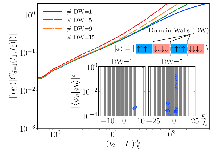
Figure 3: Hierarchical dynamics. By increasing the number of domain walls (DW, see sketch in the figure) in the initial state, the dynamics of the two-time correlation function evolves faster from a regime where it follows a stretched exponential towards an algebraic region. The full quantum evolution obtained by t-MPS is shown for $L=64,J_{z}=10J_{x},\hbar\gamma=2J_{x}$ and $t_{1}J_{x}=5\hbar$. The inset shows the overlap (blue circles) of initial states with different numbers of domain walls with the energy eigenstates (grey vertical lines) of $H_{\text{XXZ}}$ computed with exact diagonalization for a system of size $L=12$ (with open boundary conditions) and $J_{z}=10J_{x}$.

In summary, considering the evolution of two-time correlations, we highlighted the extremely rich and intricate physics at play in strongly interacting systems in contact with an environment. We evaluated quasi-exactly for the first time these correlations along all spin directions extending dissipative MPS to two-time correlations, and showed that their evolution is non-trivially affected by the presence of a dissipative coupling, even leading to the breakdown of time-translation invariance. Perhaps most importantly, we demonstrated that the dissipative heating dynamics reveals fundamental spectral features of the underlying Hamiltonian. This finding paves the way to the development of non-equilibrium techniques to probe the spectrum of strongly correlated many-body systems.

Acknowledgments: We thank I. Lesanovsky and M. Fleischhauer for enlighting discussions. We acknowledge support from Shahid Beheshti University, G.C. (A.S.), Singapore Ministry of Education (D.P.), Singapore Academic Research Fund Tier-II (project MOE2016-T2-1-065, WBS R-144-000-350-112) (D.P.) and DFG (TR 185 project B4, SFB 1238 project C05, and Einzelantrag) and the ERC (Grant Number 648166) (C.K.).

.1 Adiabatic elimination formalism

At sufficiently large times, irrespective of the spin-spin interaction strength, the dissipation-free subspace will be reached. While this subspace is highly degenerate with respect to the dissipator, the Hamiltonian can possibly lift this degeneracy. In order to understand the non-equilibrium dynamics taking place, we perform adiabatic elimination revealing how spin-flip induced virtual excitations around the dissipation-free subspace affect the evolution of the system. For the system under study, in the presence of periodic boundary conditions, the dissipation-free subspace can be written down as $\rho_{0}=\sum_{\vec{\sigma}}\rho_{0,\vec{\sigma}}|\vec{\sigma}\rangle\langle\vec{\sigma}|$ where the different spin configurations are labeled within the $z$-component basis such that $\vec{\sigma}=(\sigma_{1},\sigma_{2},\cdots,\sigma_{L})$ with $\sigma_{l}=\pm 1/2$. For times larger than $1/\gamma$, the density matrix evolution is then effectively described by the set of differential equations

$$\frac{\partial\rho_{0,\vec{\sigma}}}{\partial t}=\sum_{j=1}^{L}\frac{J_{x}^{2}\gamma}{2\left[\left(J_{z}\alpha_{j}\right)^{2}+\left(\hbar\gamma\right)^{2}\right]}\delta_{\sigma_{j},\bar{\sigma}_{j+1}}\left(\rho_{0,\vec{\sigma}_{j}}-\rho_{0,\vec{\sigma}}\right),$$

where $\alpha_{j}=2(\sigma_{j-1}\sigma_{j}+\sigma_{j+1}\sigma_{j+2})$, $\vec{\sigma}_{j}$ is the spin configuration $\vec{\sigma}$ with swapped spins at site $j$ and $j+1$ and $\bar{\sigma}_{j}=-\sigma_{j}$.

.2 Equal-time correlations

Within adiabatic elimination, the equal-time correlations can be calculated in two different ways. Using kinetic Monte Carlo, we can solve numerically for $\rho_{0}$ and then compute the correlations. While in a second approach, valid for $\hbar\gamma\gg J_{z}$, we use the differential equation found above for $\rho_{0}$ to write down a set of coupled differential equations for $\hbar^{2}C_{j,j+d}(t_{1},t_{1})=\langle S^{z}_{j}(t_{1})S^{z}_{j+d}(t_{1})\rangle$. Together with periodic boundary conditions, these equations take the form

$$\frac{\partial}{\partial t_{1}}C_{j,j\pm 1}(t_{1},t_{1}) =\frac{D}{2}\left(C_{j\mp 1,j\pm 1}+C_{j,j\pm 2}-2C_{j,j\pm 1}\right),$$

$$\frac{\partial}{\partial t_{1}}C_{j,j+d}(t_{1},t_{1}) =\frac{D}{2}\left(C_{j+1,j+d}+C_{j-1,j+d}+C_{j,j+d+1}\right.$$

$$\qquad\left.+~{}C_{j,j+d-1}-4C_{j,j+d}\right),~{}~{}~{}~{}\text{for $|d|>1$},$$

where $D=\frac{J_{x}^{2}}{\hbar^{2}\gamma}$ and here $C_{l,l+d}$ stands for $C_{l,l+d}(t_{1},t_{1})$. If the system is initially prepared in the Néel state, the correlations are translationally invariant, $C_{d}(t_{1},t_{1})=C_{j,j+d}(t_{1},t_{1})$ with equations

$$\frac{\partial}{\partial t_{1}}C_{\pm 1}(t_{1},t_{1}) =D\left(C_{\pm 2}-C_{\pm 1}\right),$$

$$\frac{\partial}{\partial t_{1}}C_{d}(t_{1},t_{1}) =D\left(C_{d+1}+C_{d-1}-2C_{d}\right),~{}~{}~{}~{}\text{for $|d|>1$},$$

and one should note that $C_{d}=C_{-d}$. To solve this system of differential equations, it is advantageous to redefine the equal-time correlations such that the evolution for all distances is decribed by an differential equation of the same form. To do so, we redefine the correlations as $\tilde{C}_{d}(t_{1},t_{1})=C_{d}(t_{1},t_{1})$ for $d\geq 1$ and $\tilde{C}_{d+1}(t_{1},t_{1})=C_{d}(t_{1},t_{1})$ for $d\leq-1$ implying that $\tilde{C}_{d}(t_{1},t_{1})=\tilde{C}_{-d+1}(t_{1},t_{1})$ for $d\geq 1$. One can then write down a diffusion equation for $\tilde{C}_{d}$ with diffusion constant $D$ and periodic boundary condition

$$\frac{\partial}{\partial t_{1}}\tilde{C}_{d}(t_{1},t_{1})=D\left(\tilde{C}_{d+1}+\tilde{C}_{d-1}-2\tilde{C}_{d}\right)$$

valid for $-\frac{L}{2}+2\leq d\leq\frac{L}{2}$. This equation can be solved analytically in terms of the modified Bessel functions $I_{n}(x)$, and has for solution

$$\tilde{C}_{d}(t_{1},t_{1})=\frac{1}{4}e^{-2Dt_{1}}~{}~{}\times$$

$$\quad\left(-I_{d}(2Dt_{1})+\sum_{j=-\frac{L}{2}+2}^{\frac{L}{2}}(-1)^{j}\text{sign}(j)I_{d-j}(2Dt_{1})\right).$$

For $d\geq 1$, in the limit where $L\gg 1$, the equal-time correlations take the form

$$C_{d}(t_{1},t_{1})=\frac{(-1)^{d}}{4}e^{-2Dt_{1}}\sum_{j=1-d}^{d-1}(-1)^{j}I_{j}(2Dt_{1}),$$ (2)

and, furthermore, in the long-time limit, $Dt_{1}\gg 1$, when $I_{n}(x)\sim e^{x}/\sqrt{2\pi x}$, these correlations simplify to

$$C_{d}(t_{1},t_{1})\sim-\frac{1}{\sqrt{64\pi Dt_{1}}}.$$

Therefore, equal-time correlations scale in time as $t_{1}^{-1/2}$ in agreement with t-MPS simulations as seen in Fig. (1) (a). In fact, due to the form of the differential equations, one can infer that equal-time correlations propagate diffusively under the action of the dephasing environment. In Fig. (1) (b), one sees that all three methods, kinetic Monte Carlo, analytical adiabatic elimination and t-MPS, predict the same scaling behavior at large times. While parallel, the analytical curve appears slightly below the two other ones, this discrepancy arises as obtaining an analytical solution requires to set $J_{z}=0$. However, even for finite $J_{z}$, the agreement between the analytical and the two other solutions gets better as the ratio $\hbar\gamma/J_{z}$ increases.

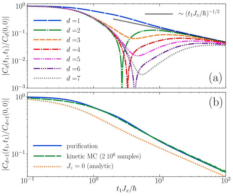
Figure 1: Equal-time correlations. Panel (a) shows the approach of a regime with diffusive dynamics for the normalized equal-time correlations, $|C_{d}(t_{1},t_{1})/C_{d}(0,0)|$, for spins separated by different distances $d$ where $\hbar^{2}C_{d}(t_{1},t_{1})=\langle S^{z}_{\frac{L}{2}}(t_{1})S^{z}_{\frac{L}{2}+d}(t_{1})\rangle$. The thin dotted black line is a guide to the eye highlighting the scaling at long times. Panel (b) compares the full quantum evolution of the density matrix, with a kinetic Monte Carlo simulation of the evolution within the dissipation-free subspace, and with the solution obtained by solving the differential equations presented at Eq. (LABEL:eq:diffusion1t). Parameters are $\hbar\gamma=2J_{x},L=80$ and $J_{z}=2J_{x}$.

.3 Two-time correlations

The long-time scaling of two-time correlations can also be understood analytically. In this case, to make progress, one needs to resort to adiabatic elimination and also make use of the quantum regression theorem Gardiner and Zoller (2000); Breuer and Petruccione (2002). As within adiabatic elimination, for times larger than $1/\gamma$ and for $\hbar\gamma\gg J_{z}$, the evolution of $\langle S^{z}_{j}(t)\rangle$ is governed by the linear differential equation

$$\frac{\partial}{\partial t_{1}}\langle S^{z}_{j}\rangle =\frac{D}{2}\sum_{l=1}^{L}\left(\delta_{j+1,l}+\delta_{j-1,l}-2\delta_{j,l}\right)\langle S^{z}_{l}\rangle$$

$$=\sum_{l=1}^{L}G_{j,l}~{}\langle S^{z}_{l}\rangle,$$ (3)

the quantum regression theorem states that the two-time correlation functions

$$\hbar^{2}C_{j,j+d}(t_{1}+\tau,t_{1})=\langle S^{z}_{j}(t_{1}+\tau)S^{z}_{j+d}(t_{1})\rangle$$

should be described by the differential equations

$$\frac{\partial}{\partial\tau}C_{j,j+d}(t_{1}+\tau,t_{1}) = \sum_{l=1}^{L}G_{j,l}~{}C_{l,j+d}(t_{1}+\tau,t_{1})$$

where $G_{j,l}$ are the same matrix elements as in Eq. (3). Assuming once again spatial translation invariance this set of equations reduces to a smaller set of diffusive equations for $C_{d}(t_{1}+\tau,t_{1})$ with diffusion constant $\frac{D}{2}$,

$$\frac{\partial}{\partial\tau}C_{d}(t_{1}+\tau,t_{1})=\frac{D}{2}(C_{d+1}+C_{d-1}-2C_{d}),$$

here $C_{l}$ stands for $C_{l}(t_{1}+\tau,t_{1})$. Solving this set of differential equations, we find the two-time correlations along the $z$-direction to evolve as

$$C_{d}(t_{2},t_{1}) =e^{-D(t_{2}-t_{1})}~{}~{}\times$$

$$\quad\quad\sum_{d^{\prime}=-\frac{L}{2}+1}^{\frac{L}{2}}C_{d^{\prime}}(t_{1},t_{1})~{}I_{d-d^{\prime}}(D(t_{2}-t_{1}))$$

where $t_{2}=t_{1}+\tau$. Then, using as initial conditions $C_{d}(t_{1},t_{1})$ obtained in Eq. (2) for $d\geq 1$ together with $C_{d=0}(t_{1},t_{1})=\frac{1}{4}$ and $C_{-d}(t_{1},t_{1})=C_{d}(t_{1},t_{1})$, we find for $d\geq 0$, in the limit $L\gg 1$, that the two-time correlations can be rewritten in the more amenable form

$$C_{d}(t_{2},t_{1})=\frac{1}{4}e^{-D(t_{2}-t_{1})}I_{d}(D(t_{2}-t_{1}))$$ (4)

$$-\frac{1}{4}~{}\delta_{0,d}~{}e^{-D(t_{2}+t_{1})}I_{0}(D(t_{2}+t_{1}))$$

$$+\frac{(-1)^{d}}{4}(1-\delta_{0,d})~{}e^{-D(t_{2}+t_{1})}\sum_{j=1-d}^{d-1}(-1)^{j}I_{j}(D(t_{2}+t_{1}))$$

$$+G_{d}(t_{2},t_{1}),$$

where

$$G_{d}(t_{2},t_{1}) =e^{-D(t_{2}-t_{1})}\sum_{d^{\prime}=1}^{\infty}C_{d^{\prime}}(t_{1},t_{1})$$ (5)

$$\times~{}(I_{d+d^{\prime}}(D(t_{2}-t_{1}))-I_{d+d^{\prime}-1}(D(t_{2}-t_{1}))).$$

Using this expression, we then evaluate the scaling of the normalized two-time correlations in the limit $Dt_{2}\gg Dt_{1}\gg 1$. While for the first three terms of Eq. (4), we simply expand $I_{n}(x)$ for large $x$, for $G_{d}(t_{1},t_{2})$, we also need to take the continuum limit in order to carry out analytically the sum over $d^{\prime}$. This additional limit amounts to approximate $C_{d^{\prime}}(t_{1},t_{1})$ in Eq. (5) as

$$C_{d^{\prime}}(t_{1},t_{1})\sim-\frac{1}{4}\frac{1}{\sqrt{2\pi(2Dt_{1})}}~{}e^{-\frac{1}{2}\frac{d^{\prime 2}}{2Dt_{1}}}.$$

For $|d|\geq 1$, the normalized two-time correlations therefore scale as

$$\frac{C_{d}(t_{2},t_{1})}{C_{d}(t_{1},t_{1})}\sim -\sqrt{2}~{}\left(\frac{t_{2}}{t_{1}}\right)^{-\frac{3}{2}}\times$$

$$\left(1+\frac{1}{\sqrt{\pi}}(Dt_{1})^{-\frac{1}{2}}-\frac{1}{4}(Dt_{1})^{-1}\right).$$

Thus, for very large $Dt_{1}$, only the leading contribution remains and the normalized two-time correlations scale as

$$\left|\frac{C_{d}(t_{2},t_{1})}{C_{d}(t_{1},t_{1})}\right|\sim\sqrt{2}\left(\frac{t_{2}}{t_{1}}\right)^{-\frac{3}{2}},\quad|d|\geq 1,$$

which is in agreement with the results obtained from t-MPS. This result highlights that aging dynamics can emerge from diffusive processes triggered by dephasing noise. Finally, for $d=0$, where $C_{0}(t_{1},t_{1})=\frac{1}{4}$, the long-time limit of the normalized two-time correlation scale as

$$\frac{C_{0}(t_{2},t_{1})}{C_{0}(t_{1},t_{1})}\sim \frac{1}{\sqrt{2\pi}}~{}(Dt_{1})^{-\frac{1}{2}}\left(\frac{t_{2}}{t_{1}}\right)^{-\frac{3}{2}}\times$$

$$\left(1+\frac{1}{\sqrt{\pi}}(Dt_{1})^{-\frac{1}{2}}-\frac{1}{4}(Dt_{1})^{-1}\right).$$

Consequently, on-site two-time correlations break time-translational invariance and scale algebraically; however, to leading order, these correlations do not solely depend on the ratio $t_{2}/t_{1}$ and thus do not display aging.

References

- Lu et al. (2012) D. Lu, I. M. Vishik, M. Yi, Y. Chen, R. G. Moore, and Z.-X. Shen, Annual Review of Condensed Matter Physics 3, 129 (2012) .
- Bramwell and Keimer (2014) S. T. Bramwell and B. Keimer, Nature Materials 13, 763 (2014).
- Ashcroft and Mermin (1976) N. W. Ashcroft and N. D. Mermin, Solid State Physics (Thomson Learning, 1976).
- Stewart et al. (2008) J. T. Stewart, J. P. Gaebler, and D. S. Jin, Nature 454, 744 (2008).
- Esslinger (2010) T. Esslinger, Annual Review of Condensed Matter Physics 1, 129 (2010) .
- Stöferle et al. (2004) T. Stöferle, H. Moritz, C. Schori, M. Köhl, and T. Esslinger, Phys. Rev. Lett. 92, 130403 (2004).
- Vincent and Dupuis (2017) E. Vincent and V. Dupuis, arXiv:1709.10293 (2017).
- Marino and Silva (2012) J. Marino and A. Silva, Phys. Rev. B 86, 060408 (2012).
- Bernier et al. (2018) J.-S. Bernier, R. Tan, L. Bonnes, C. Guo, D. Poletti, and C. Kollath, Phys. Rev. Lett. 120, 020401 (2018).
- Buchhold and Diehl (2015) M. Buchhold and S. Diehl, Phys. Rev. A 92, 013603 (2015).
- Marcuzzi et al. (2015) M. Marcuzzi, E. Levi, W. Li, J. P. Garrahan, B. Olmos, and I. Lesanovsky, New Journal of Physics 17, 072003 (2015).
- Sciolla et al. (2015) B. Sciolla, D. Poletti, and C. Kollath, Phys. Rev. Lett. 114, 170401 (2015).
- Everest et al. (2017) B. Everest, I. Lesanovsky, J. P. Garrahan, and E. Levi, Phys. Rev. B 95, 024310 (2017).
- He et al. (2017) L. He, L. M. Sieberer, and S. Diehl, Phys. Rev. Lett. 118, 085301 (2017).
- (15) Z. Denis and S. Wimberger, Cond. Matt. 3, 2 (2018).
- Wang et al. (2018) R. R. W. Wang, B. Xing, G. G. Carlo, and D. Poletti, Phys. Rev. E 97, 020202 (2018).
- Cai and Barthel (2013) Z. Cai and T. Barthel, Phys. Rev. Lett. 111, 150403 (2013).
- Poletti et al. (2012) D. Poletti, J.-S. Bernier, A. Georges, and C. Kollath, Phys. Rev. Lett. 109, 045302 (2012).
- Poletti et al. (2013) D. Poletti, P. Barmettler, A. Georges, and C. Kollath, Phys. Rev. Lett. 111, 195301 (2013).
- White (1992) S. R. White, Phys. Rev. Lett. 69, 2863 (1992).
- Schollwöck (2011) U. Schollwöck, Annals of Physics 326, 96 (2011), january 2011 Special Issue.
- (22) ITensor C++ library, available at http://itensor.org.
- Zwolak and Vidal (2004) M. Zwolak and G. Vidal, Phys. Rev. Lett. 93, 207205 (2004).
- Verstraete et al. (2009) F. Verstraete, M. M. Wolf, and J. I. Cirac, Nature Physics 5, 633 (2009).
- Bonnes and Läuchli (2014) L. Bonnes and A. M. Läuchli, arXiv:1411.4831 (2014).
- Mikeska and Kolezhuk (2004) H. J. Mikeska and A. Kolezhuk, in Quantum magnetism, Vol. 645, edited by U. Schollwöck, J. Richter, D. Farnell, and R. Bishop (Springer, Lecture notes in Physics, 2004) p. 1.
- Garcia-Ripoll et al. (2009) J. J. Garcia-Ripoll, S. Dürr, N. Syassen, D. M. Bauer, M. Lettner, G. Rempe, and J. I. Cirac, New Journal of Physics 11, 013053 (2009).
- Gardiner and Zoller (2000) C. Gardiner and P. Zoller, Quantum Noise (Spinger-Verlag, 2000).
- Breuer and Petruccione (2002) H. P. Breuer and F. Petruccione, The theory of open quantum systems (Oxford University Press, Oxford, 2002).
- (30) See Eq. (1) of the Supplemental material.
Supplemental material

References

- Gardiner and Zoller (2000) C. Gardiner and P. Zoller, Quantum Noise (Spinger-Verlag, 2000).
- Breuer and Petruccione (2002) H. P. Breuer and F. Petruccione, The theory of open quantum systems (Oxford University Press, Oxford, 2002).