Symmetry Exploits for Bayesian Cubature Methods

Abstract

Bayesian cubature provides a flexible framework for numerical integration, in which a priori knowledge on the integrand can be encoded and exploited. This additional flexibility, compared to many classical cubature methods, comes at a computational cost which is cubic in the number of evaluations of the integrand. It has been recently observed that fully symmetric point sets can be exploited in order to reduce – in some cases substantially – the computational cost of the standard Bayesian cubature method. This work identifies several additional symmetry exploits within the Bayesian cubature framework. In particular, we go beyond earlier work in considering non-symmetric measures and, in addition to the standard Bayesian cubature method, present exploits for the Bayes–Sard cubature method and the multi-output Bayesian cubature method.

1 Introduction

This paper considers the numerical approximation of an integral

$$I(f^{\dagger})\coloneqq\int_{M}f^{\dagger}(\boldsymbol{x})\mathrm{d}\nu(\boldsymbol{x}),$$

where $(M,\mathcal{B},\nu)$ is a Borel probability space with $M$ any Borel measurable non-empty subset of $\mathbb{R}^{m}$ and $f^{\dagger}\colon M\rightarrow\mathbb{R}$ is a $\mathcal{B}$-measurable scalar-valued integrand (vector-valued integrands will be considered in Section 4). Additional assumptions will be made when necessary. Our interest is in the situation where the exact values of $f^{\dagger}$ cannot be deduced until the function itself is evaluated, and that the evaluations are associated with a substantial computational cost or a very large number of them is required. Such situations are typical in, for example, uncertainty quantification for chemical systems Najm2009 , fluid mechanical simulation Xiu2003 and certain financial applications Holtz2011 .

In the presence of a limited computational budget, it is natural to exploit any contextual information that may be available on the integrand. Classical cubatures, such as spline-based or Gaussian cubatures, are able to exploit abstract mathematical information, such as the number of continuous derivatives of the integrand Davis2007 . However, in situations where more detailed or specific contextual information is available to the analyst, the use of generic classical cubatures can be sub-optimal.

The language of probabilities provides one mechanism in which contextual information about the integrand can be captured. Let $(\Omega,\mathcal{F},\mathbb{P})$ be a probability space. Then an analyst can elicit their prior information about the integrand $f^{\dagger}$ in the form of a stochastic process model

$$\omega\mapsto f(\cdot\,;\omega),\qquad\omega\in\Omega,$$ (1)

wherein the function $\boldsymbol{x}\mapsto f(\boldsymbol{x};\omega)$ is $\mathcal{B}$-measurable for each fixed $\omega\in\Omega$. Through the stochastic process, the analyst can encode both abstract mathematical information, such as the number of continuous derivatives of the integrand, and specific contextual information, such as the possibility of a trend or a periodic component. The process of elicitation is not discussed in this work (see Diaconis1988 ; Hennig2015 ); for our purposes the stochastic process in (1) is considered to be provided.

In Bayesian cubature methods, due to Larkin Larkin1972 and re-discovered in Diaconis1988 ; OHagan1991 ; Minka2000 , the analyst first selects a point set $X=\{\boldsymbol{x}_{i}\}_{i=1}^{N}\subset M$, $N\in\mathbb{N}$, on which the true integrand $f^{\dagger}$ is evaluated. Let this data be denoted $\mathcal{D}=\{(\boldsymbol{x}_{i},f^{\dagger}(\boldsymbol{x}_{i}))\}_{i=1}^{N}$. Then the analyst conditions their stochastic process according to these data $\mathcal{D}$, to obtain a second stochastic process

$$\omega\mapsto f_{N}(\cdot\,;\omega).$$

The analyst reports the implied distribution over the value of the integral of interest; that is the law of the random variable

$$\omega\mapsto\int_{M}f_{N}(\boldsymbol{x};\omega)\mathrm{d}\nu(\boldsymbol{x}).$$

This distribution can be computed in closed form under certain assumptions on the structure of the prior model. A sufficient condition is that the stochastic process is Gaussian, which (arguably) does not severely restrict the analyst in terms of what contextual information can be included Rasmussen2006 . In addition, the probabilistic output of the method enables uncertainty quantification for the unknown true value of the integral Larkin1972 ; Cockayne2017 ; Briol2017 . These appealing properties have led to Bayesian cubature methods being used in diverse areas such as from computer graphics Marques2013 , non-linear filtering Prueher2017 and applied Bayesian statistics Osborne2012 .

The theoretical aspects of Bayesian cubature methods have now been widely-studied. In particular, convergence of the posterior mean point estimator

$$\int_{\Omega}\int_{M}f_{N}(\boldsymbol{x};\omega)\mathrm{d}\nu(\boldsymbol{x})\mathrm{d}\mathbb{P}(\omega)\rightarrow\int_{M}f^{\dagger}(\boldsymbol{x})\mathrm{d}\nu(\boldsymbol{x})$$ (2)

as $N\rightarrow\infty$ has been studied in both the well-specified Bezhaev1991 ; SommarivaVianello2006 ; Briol2015 ; Ehler2018 ; Briol2017 and mis-specified Kanagawa2016 ; Kanagawa2017 regimes. Some relationships between the posterior mean estimator and classical cubature methods have been documented in Diaconis1988 ; Sarkka2016 ; Karvonen2017a . In Larkin1974 ; OHagan1991 ; Karvonen2018c the Bayes–Sard framework was studied, where it was proposed to incorporate an explicit parametric component OHagan1978 into the prior model in order that contextual information, such as trends, can be properly encoded. The choice of point set $X$ for Bayesian cubature has been studied in Briol2015 ; Bach2017 ; Briol2017a ; Oettershagen2017 ; Chen2018 ; Pronzato2018 . In addition, several extensions have been considered to address specific technical challenges posed by non-negative integrands Chai2018 , model evidence integrals in a Bayesian context Osborne2012 ; Gunter2014 , ratios Osborne2012a , non-Gaussian prior models Kennedy1998 ; Prueher2017 , measures that can be only be sampled Oates2017 , and vector-valued integrands Xi2018 .

Despite these recent successes, a significant drawback of Bayesian cubature methods is that the cost of computing the distributional output is typically cubic in $N$, the size of the point set. For integrals whose domain $M$ is high-dimensional, the number $N$ of points required can be exponential in $m=\text{dim}(M)$. Thus the cubic cost associated with Bayesian cubature methods can render them impractical. In recent work, Karvonen and Särkkä Karvonen2018 noted that symmetric structure in the point set can be exploited to reduce the total computational cost. Indeed, in some cases the exponential dependence on $m$ can be reduced to (approximately) linear. This is a similar effect to that achieved in the circulant embedding approach Dietrich1997 , or by the use of $\mathcal{H}$-matrices Hackbusch1999 and related approximations Schaefer2017 , though the approaches differ at a fundamental level. The aim of this paper is to present several related symmetry exploits that are specifically designed to reduce computational cost of Bayesian cubature methods.

Our principal contributions are following: First, the techniques developed in Karvonen2018 are extended to the Bayes–Sard cubature method. This results in a computational method that is, essentially, of the complexity ${\mathcal{O}(J^{3}+JN)}$, where $J$ is the number of symmetric sets that constitute the full point set, instead of being cubic in $N$. In typical scenarios there are at most a few hundred symmetric sets even though the total number of points can go up to millions. Second, we present an extension to the multi-output (i.e., vector-valued) Bayesian cubature method that is used to simultaneously integrate $D\in\mathbb{N}$ related integrals. In this case, the computational complexity is reduced from $\mathcal{O}(D^{3}N^{3})$ to $\mathcal{O}(D^{3}J^{3}+DJN)$. Third, a symmetric change of measure technique is proposed to avoid the (strong) assumption of symmetry on the measure $\nu$ that was required in Karvonen2018 . Fourth, the performance of our techniques is empirically explored. Throughout, our focus is not on the performance of these integration methods, which has been explored in earlier work, already cited. Rather, our focus is on how computation for these methods can be accelerated.

The remainder of the article is structured as follows: Section 2 covers the essential background for Bayesian cubature methods and introduces fully symmetric sets that are used in the symmetry exploits throughout the article. Sections 3 and 4 develop fully symmetric Bayes–Sard cubature and fully symmetric multi-output Bayesian cubature. Section 5 explains how the assumption that $\nu$ is symmetric can be relaxed. In Section 6 a detailed selection of empirical results are presented. Finally, some concluding remarks and discussion are contained in Section 7.

2 Background

This section reviews the standard Bayesian cubature method, due to Larkin Larkin1972 , and explains how fully symmetric sets can be used to alleviate its computational cost, as proposed in Karvonen2018 .

2.1 Standard Bayesian Cubature

In this section we present explicit formulae for the Bayesian cubature method in the case where the prior model (1) is a Gaussian random field. To simplify the notation, Sections 2 and 3 assume that the integrand has scalar output (i.e. $D=1$); this is then extended to vector-valued output in Section 4.

To reduce the notational overhead, in what follows the $\omega\in\Omega$ argument is left implicit. Thus we consider $f(\boldsymbol{x})$ to be a scalar-valued random variable for each $\boldsymbol{x}\in M$. In particular, in this paper we focus on stochastic processes that are Gaussian, meaning that there exists a mean function $m\mathrel{\mathop{\ordinarycolon}}M\rightarrow\mathbb{R}$ and a symmetric positive definite covariance function (or kernel) $k\mathrel{\mathop{\ordinarycolon}}M\times M\rightarrow\mathbb{R}$ such that $[f(\boldsymbol{x}_{1}),\ldots,f(\boldsymbol{x}_{N})]^{\textsf{T}}\in\mathbb{R}^{N}$ has the multivariate Gaussian distribution

$$\mathrm{N}\left(\begin{bmatrix}m(\boldsymbol{x}_{1})\\ \vdots\\ m(\boldsymbol{x}_{N})\end{bmatrix},\begin{bmatrix}k(\boldsymbol{x}_{1},\boldsymbol{x}_{1})&\cdots&k(\boldsymbol{x}_{1},\boldsymbol{x}_{N})\\ \vdots&\ddots&\vdots\\ k(\boldsymbol{x}_{N},\boldsymbol{x}_{1})&\cdots&k(\boldsymbol{x}_{N},\boldsymbol{x}_{N})\end{bmatrix}\right)$$

for any $N\in\mathbb{N}$ and all point sets $\{\boldsymbol{x}_{i}\}_{i=1}^{N}\subset M$. We assume that $\int_{M}k(\boldsymbol{x},\boldsymbol{x})\operatorname{d\!}\nu(\boldsymbol{x})<\infty$.

The conditional distribution $f_{N}$ of this field, based on the data $\mathcal{D}=\{(\boldsymbol{x}_{i},f^{\dagger}(\boldsymbol{x}_{i})\}_{i=1}^{N}$ of function evaluations at the points $X=\{\boldsymbol{x}_{i}\}_{i=1}^{N}$, is also Gaussian, with mean and covariance functions

$$m_{N}(\boldsymbol{x}) =m(\boldsymbol{x})+\boldsymbol{k}_{X}(\boldsymbol{x})^{\textsf{T}}\boldsymbol{K}_{X}^{-1}(\boldsymbol{f}^{\dagger}_{X}-\boldsymbol{m}_{X}),$$ (3)

$$k_{N}(\boldsymbol{x},\boldsymbol{x}^{\prime}) =k(\boldsymbol{x},\boldsymbol{x}^{\prime})-\boldsymbol{k}_{X}(\boldsymbol{x})^{\textsf{T}}\boldsymbol{K}_{X}^{-1}\boldsymbol{k}_{X}(\boldsymbol{x}^{\prime}),$$ (4)

where the vector $\boldsymbol{f}^{\dagger}_{X}\in\mathbb{R}^{N}$ contains evaluations of the integrand, $[\boldsymbol{f}^{\dagger}_{X}]_{i}=f^{\dagger}(\boldsymbol{x}_{i})$, the vector $\boldsymbol{m}_{X}\in\mathbb{R}^{N}$ contains evaluations of the prior mean, $[\boldsymbol{m}_{X}]_{i}=m(\boldsymbol{x}_{i})$, the vector $\boldsymbol{k}_{X}(\boldsymbol{x})\in\mathbb{R}^{N}$ contains evaluations of the kernel, $[\boldsymbol{k}_{X}(\boldsymbol{x})]_{i}=k(\boldsymbol{x},\boldsymbol{x}_{i})$, and $\boldsymbol{K}_{X}=\boldsymbol{K}_{X,X}\in\mathbb{R}^{N\times N}$ is the kernel matrix, $[\boldsymbol{K}_{X}]_{ij}=k(\boldsymbol{x}_{i},\boldsymbol{x}_{j})$. From the fact that linear functionals of Gaussian processes are Gaussian, we obtain that

$$\int_{M}f_{N}(\boldsymbol{x})\operatorname{d\!}\nu(\boldsymbol{x})\sim\mathrm{N}\big{(}\mu_{N}(f^{\dagger}),\sigma_{N}^{2}\big{)},$$ (5)

with

$$\mu_{N}(f^{\dagger})={} I(m)+\boldsymbol{k}_{\nu,X}^{\textsf{T}}\boldsymbol{K}_{X}^{-1}(\boldsymbol{f}^{\dagger}_{X}-\boldsymbol{m}_{X}),$$ (6)

$$\sigma_{N}^{2}={} k_{\nu,\nu}-\boldsymbol{k}_{\nu,X}^{\textsf{T}}\boldsymbol{K}_{X}^{-1}\boldsymbol{k}_{\nu,X}.$$ (7)

Here $k_{\nu}(\boldsymbol{x})\mathrel{\mathop{\ordinarycolon}}=\int_{M}k(\boldsymbol{x},\boldsymbol{x}^{\prime})\operatorname{d\!}\nu(\boldsymbol{x}^{\prime})$ is called the kernel mean function Smola2007 and $\boldsymbol{k}_{\nu,X}\in\mathbb{R}^{N}$ is the column vector with $[\boldsymbol{k}_{\nu,X}]_{i}=k_{\nu}(\boldsymbol{x}_{i})$, whilst $k_{\nu,\nu}\mathrel{\mathop{\ordinarycolon}}=\int_{M}k_{\nu}(\boldsymbol{x})\operatorname{d\!}\nu(\boldsymbol{x})\geq 0$ is the variance of the integral itself under the prior model. The assumption $\int_{M}k(\boldsymbol{x},\boldsymbol{x})\operatorname{d\!}\nu(\boldsymbol{x})<\infty$ guarantees that the kernel mean is finite. This method is known as the standard Bayesian cubature, with the implicit understanding that the model for the integrand should be carefully selected to ensure (5) is well-calibrated Briol2017 , meaning that the uncertainty assessment can be trusted. The need for careful calibration is in line with standard approaches to the Gaussian process regression task Rasmussen2006 .

To understand when the Bayesian cubature output is meaningful, it is useful to write the posterior mean and variance (6) and (7) in terms of the weight vector

$$\boldsymbol{w}_{X}\coloneqq\boldsymbol{K}_{X}^{-1}\boldsymbol{k}_{\nu,X}.$$ (8)

That is, we have $\mu_{N}(f^{\dagger})=I(m)+\boldsymbol{w}_{X}^{\textsf{T}}(\boldsymbol{f}_{X}^{\dagger}-\boldsymbol{m}_{X})$ and $\sigma_{N}^{2}=k_{\nu,\nu}-\boldsymbol{w}_{X}^{\textsf{T}}\boldsymbol{k}_{\nu,X}$. Let $\mathcal{H}(k)$ be the Hilbert space reproduced by the kernel $k$ (see Berlinet2011 for background). It can then be verified that $\boldsymbol{w}_{X}$ solves a quadratic minimisation problem of approximating $k_{\nu}$ with a function from the finite-dimensional space spanned by ${\{k(\cdot,\boldsymbol{x})\}_{\boldsymbol{x}\in X}\subset\mathcal{H}(k)}$, namely:

$$\boldsymbol{w}_{X}=\operatorname*{arg\,min}_{\boldsymbol{w}\in\mathbb{R}^{N}}\bigg{\|}k_{\nu}(\cdot)-\sum_{i=1}^{N}w_{i}k(\cdot,\boldsymbol{x}_{i})\bigg{\|}_{\mathcal{H}(k)}.$$

and that the minimum the value of this norm is $\sigma_{X}$ (see e.g. (Oettershagen2017, , Ch. 3) and Bach2012 ). Equivalently, the weight vector can be obtained as the minimiser of the worst case error

$$\sup_{\|f^{\dagger}\|_{\mathcal{H}(k)}\leq 1}\mathinner{\!\biggl{\lvert}\int_{M}f^{\dagger}(\boldsymbol{x})\operatorname{d\!}\nu(\boldsymbol{x})-\sum_{i=1}^{N}w_{i}f^{\dagger}(\boldsymbol{x}_{i})\biggr{\rvert}}$$

among all cubature rules with points $X$, with $\sigma_{N}$ corresponding to the minimal worst case error Briol2017 ; Oettershagen2017 . Thus, in terms of uncertainty quantification, the posterior standard deviation $\sigma_{X}$ can indeed be meaningfully related to the integration problem being solved.

The principal motivation for this work is the observation that both (6) and (7) involve the solution of an $N$-dimensional linear system defined by the matrix $\boldsymbol{K}_{X}$. In general this is a dense matrix and, as such, in the absence of additional structure in the linear system Karvonen2018 or further approximations (e.g. LazaroGredilla2010 ; Hensman2018 ; Schaefer2017 ), the computational complexity associated with the standard Bayesian cubature method is $\mathcal{O}(N^{3})$. Moreover, it is often the case that $\boldsymbol{K}_{X}$ is ill-conditioned Schaback1995 ; Stein2012 . The exploitation of symmetric structure to circumvent the solution of a large and ill-conditioned linear system would render Bayesian cubature more practical, in the sense of computational efficiency and numerical robustness; this is the contribution of the present article.

2.2 Symmetry Properties

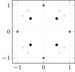
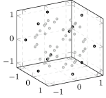
Figure 1: Fully symmetric sets generated by the vectors $[0.5,0.5]$, $[1,0]$, and $[0.6,0.8]$ in $\mathbb{R}^{2}$ (left) and $[1,1,0]$ and $[0.2,0.6,0.8]$ in $\mathbb{R}^{3}$ (right).

Next we introduce fully symmetric sets and related symmetry concepts, before explaining in Section 2.3 how these can be exploited for computational simplification in the standard Bayesian cubature method. Note that, in what follows, no symmetry properties are needed for the integrand $f^{\dagger}$ itself.

2.2.1 Fully Symmetric Point Sets

Given a vector $\boldsymbol{\lambda}\in\mathbb{R}^{m}$, the fully symmetric set $[\boldsymbol{\lambda}]\subset\mathbb{R}^{m}$ generated by this vector is defined as the point set consisting of all vectors that can be obtained from $\boldsymbol{\lambda}$ via coordinate permutations and sign changes. That is,

$$\begin{split}[\boldsymbol{\lambda}]&=[\lambda_{1},\ldots,\lambda_{d}]\\ &\coloneqq\bigcup_{q\in\Pi_{m}}\bigcup_{\boldsymbol{s}\in S_{m}}\big{\{}(s_{1}\lambda_{q_{1}},\ldots,s_{d}\lambda_{q_{d}}\big{\}}\subset\mathbb{R}^{m},\end{split}$$

where $\Pi_{m}$ and $S_{m}$ stand for the collections of all permutations of the first $m$ positive integers and of all vectors of the form $\boldsymbol{s}=(s_{1},\ldots,s_{m})$ with each $s_{i}$ either $1$ or $-1$. Here $\boldsymbol{\lambda}$ is called a generator vector and its individual elements are called generators. Alternatively, we can write the fully symmetric set in terms of permutation and sign change matrices:

$$[\boldsymbol{\lambda}]=\bigcup_{\boldsymbol{P}\in\mathrm{Perm}^{\text{\tiny{SC}}}_{m}}\boldsymbol{P}\boldsymbol{\lambda},$$

where $\mathrm{Perm}^{\text{\tiny{SC}}}_{m}$ is the collection of $m\times m$ matrices having exactly one non-zero element on each row and column, this element being either $1$ or $-1$. Some fully symmetric sets are displayed in Figure 1. The cardinality of a fully symmetric set $[\boldsymbol{\lambda}]$, generated by a generator vector $\boldsymbol{\lambda}$ containing $r_{0}$ zero generators and $l$ distinct non-zero generators with multiplicities $r_{1},\ldots,r_{l}$, is

$$\#[\boldsymbol{\lambda}]=\frac{2^{m-r_{0}}d!}{r_{0}!\cdots r_{l}!}.$$ (9)

See Table 1 for a number of examples in low dimensions.

For $\boldsymbol{\lambda}\in\mathbb{R}^{m}$ having non-negative elements, we occasionally need the concept of a non-negative fully symmetric set

$$[\boldsymbol{\lambda}]^{+}\coloneqq\bigcup_{\boldsymbol{P}\in\text{Perm}_{m}}\boldsymbol{P}\boldsymbol{\lambda}\subset\mathbb{R}^{m}_{+},$$

where $\text{Perm}_{m}\subset\mathrm{Perm}^{\text{\tiny{SC}}}_{m}$ is the collection of $m\times m$ permutation matrices.

Table 1: Sizes of fully symmetric sets generated by the generator vector $\boldsymbol{\lambda}=(\lambda_{1},\ldots,\lambda_{l},0,\ldots,0)$ having $l\leq m$ distinct non-zero elements $\lambda_{1},\ldots,\lambda_{l}$ (see (9)).

Dimension ($m$)

	2	3	4	5	6	7
$l=1$	4	6	8	10	12	14
$l=2$	8	24	48	80	120	168
$l=3$	-	48	192	480	960	1,680
$l=4$	-	-	384	1,920	5,760	13,440
$l=5$	-	-	-	3,840	23,040	80,640
$l=6$	-	-	-	-	46,080	322,560
$l=7$	-	-	-	-	-	645,120

2.2.2 Fully Symmetric Domains, Kernels, and Measures

At this point we introduce several related definitions; these enable us later to state precisely which symmetry assumptions are being exploited.

Domains.

It will be assumed in the sequel that ${M\subset\mathbb{R}^{m}}$ is a fully symmetric domain, meaning that every fully symmetric set generated by a vector from $M$ is contained in $M$: $[\boldsymbol{\lambda}]\subset M$ whenever $\boldsymbol{\lambda}\in M$. Equivalently, ${M=\boldsymbol{P}M=\{\boldsymbol{P}\boldsymbol{x}\,\colon,\boldsymbol{x}\in M\}}$ for any $\boldsymbol{P}\in\mathrm{Perm}^{\text{\tiny{SC}}}_{m}$. Most popular domains, such as the whole of $\mathbb{R}^{m}$, hypercubes of the form $[-a,a]^{m}$ (from which e.g. the unit hypercube can be obtained by simple translation and scaling), balls and spheres, are fully symmetric.

Kernels.

A kernel $k\colon M\times M\to\mathbb{R}$ defined on a fully symmetric domain $M$ is said to be a fully symmetric kernel if $k(\boldsymbol{P}\boldsymbol{x},\boldsymbol{P}\boldsymbol{x}^{\prime})=k(\boldsymbol{x},\boldsymbol{x}^{\prime})$ for any $\boldsymbol{P}\in\mathrm{Perm}^{\text{\tiny{SC}}}_{m}$. Basic examples of fully symmetric kernels include isotropic kernels and products and sums of isotropic one-dimensional kernels.

Measures.

A measure $\nu$ on a fully symmetric domain $M$ is a fully symmetric measure if it is invariant under fully symmetric pushforwards: $\boldsymbol{P}_{*}(\nu)=\nu$ for any ${\boldsymbol{P}\in\mathrm{Perm}^{\text{\tiny{SC}}}_{m}}$. If $\nu$ admits a Lebesgue density $p_{\nu}$, this condition is equivalent to $p_{\nu}(\boldsymbol{x})=p_{\nu}(\boldsymbol{P}\boldsymbol{x})$ for any $\boldsymbol{P}\in\mathrm{Perm}^{\text{\tiny{SC}}}_{m}$. Note that this is a narrow class of measures and a relaxation of this assumption is discussed in Section 5.

2.2.3 Fully Symmetric Cubature Rules

The linear functional $\mu(f^{\dagger})=\sum_{i=1}^{N}w_{i}f^{\dagger}(\boldsymbol{x}_{i})$ is said to be fully symmetric cubature rule if its point set can be written as a union of a number $J\in\mathbb{N}$ of fully symmetric sets $[\boldsymbol{\lambda}^{1}],\ldots,[\boldsymbol{\lambda}^{J}]$ and all points in each $[\boldsymbol{\lambda}^{j}]$ are assigned an equal weight. That is, a fully symmetric cubature rule is of the form

$$\mu(f^{\dagger})=\sum_{j=1}^{J}w^{\text{\tiny{FS}}}_{j}\sum_{\boldsymbol{x}\in[\boldsymbol{\lambda}^{j}]}f^{\dagger}(\boldsymbol{x})$$

for some weights $\boldsymbol{w}^{\text{\tiny{FS}}}\in\mathbb{R}^{J}$ and generator vectors ${\boldsymbol{\lambda}^{1},\ldots,\boldsymbol{\lambda}^{J}\in M}$. Because this structure typically greatly simplifies design of the weights, many classical polynomial-based cubature rules are fully symmetric McNameeStenger1967 ; Genz1986 ; GenzKeister1996 ; LuDarmofal2004 , including certain sparse grids NovakRitter1999 ; NovakRitter1999b

2.3 Fully Symmetric Bayesian Cubature

The central aim of this article is to derive generalisations for the Bayes–Sard and multi-output Bayesian cubatures of the following result from Karvonen2018 , originally developed only for the standard Bayesian cubature method.

Theorem 2.1

Consider the standard Bayesian cubature method based on a domain $M$, measure $\nu$, and kernel $k$ that are each fully symmetric and fix the mean function to be $m\equiv 0$. Suppose that the point set is a union of $J$ fully symmetric sets: $X=\bigcup_{j=1}^{J}[\boldsymbol{\lambda}^{j}]$ for some distinct generator vectors ${\Lambda=\{\boldsymbol{\lambda}^{1},\ldots,\boldsymbol{\lambda}^{J}\}\subset M}$. Then the output of the standard Bayesian cubature method can be expressed in the fully symmetric form

$$\mu_{N}(f^{\dagger}) =\sum_{j=1}^{J}w_{\Lambda,j}\sum_{\boldsymbol{x}\in[\boldsymbol{\lambda}^{j}]}f^{\dagger}(\boldsymbol{x}),$$

$$\sigma_{N}^{2} =k_{\nu,\nu}-\sum_{j=1}^{J}w_{\Lambda,j}k_{\nu}(\boldsymbol{\lambda}^{j})\#[\boldsymbol{\lambda}^{j}].$$

The weights $\boldsymbol{w}_{\Lambda}\in\mathbb{R}^{J}$ are the solution to the linear system $\boldsymbol{S}\boldsymbol{w}_{\Lambda}=\boldsymbol{k}_{\nu,\Lambda}$ of $J$ equations, where

$$[\boldsymbol{S}]_{ij}=\sum_{\boldsymbol{x}\in[\boldsymbol{\lambda}^{j}]}k(\boldsymbol{\lambda}^{i},\boldsymbol{x})\quad\text{and}\quad[\boldsymbol{k}_{\nu,\Lambda}]_{j}=k_{\nu}(\boldsymbol{\lambda}^{j}).$$

Theorem 2.1 demonstrates the principal idea; that one can exploit symmetry to reduce the number of kernel evaluations needed in the standard Bayesian cubature method from $N^{2}$ to $NJ$ and decrease the number of equations in the linear system that needs to be solved from $N$ to $J$. Since $J$ is typically considerably smaller than $N=\sum_{j=1}^{J}\#[\boldsymbol{\lambda}^{j}]$, using fully symmetric sets results in a substantial reduction in computational cost. Numerical examples in Karvonen2018 showed that sets containing up to tens of millions of points become feasible in the standard Bayesian cubature method when symmetry exploits are used. The aim of this paper is to generalise these techniques to the important cases of Bayes–Sard cubature (Section 3) and multi-output Bayesian cubature (Section 4).

Remark 1

If $\#[\boldsymbol{\lambda}^{1}]=\cdots=\#[\boldsymbol{\lambda}^{J}]$, the condition number of the matrix $\boldsymbol{S}$ in Theorem 2.1 cannot exceed that of $\boldsymbol{K}_{X}$ (similar results are available for the matrices in Theorems 3.1 and 4.1). This scenario occurs in, for instance, the numerical example of Section 6.3. To verify the claim, observe that by Lemma 4 $\boldsymbol{S}\boldsymbol{v}=\alpha\boldsymbol{v}$ implies that the block vector

$$\boldsymbol{v}^{\prime}=\begin{bmatrix}v_{1}\boldsymbol{1}_{\#[\boldsymbol{\lambda}^{1}]}\\ \vdots\\ v_{J}\boldsymbol{1}_{\#[\boldsymbol{\lambda}^{J}]}\end{bmatrix}$$

satisfies $\boldsymbol{K}_{X}\boldsymbol{v}^{\prime}=\alpha\boldsymbol{v}^{\prime}$. Consequently, the spectrum of $\boldsymbol{S}$ is a subset of that of $\boldsymbol{K}_{X}$. Furthermore, when ${\#[\boldsymbol{\lambda}^{1}]=\cdots=\#[\boldsymbol{\lambda}^{J}]}$, the matrix $\boldsymbol{S}$ is symmetric; therefore its condition number is the ratio of the largest and smallest eigenvalues. It follows that the condition number of $\boldsymbol{S}$ must be smaller or equal to that of $\boldsymbol{K}_{X}$.

3 Fully Symmetric Bayes–Sard Cubature

In this section we first review the Bayes–Sard cubature method from Karvonen2018c and then derive a generalisation of Theorem 2.1 for this method.

3.1 Bayes–Sard Cubature

In the standard Bayesian cubature method the mean function $m$ must be a priori specified. This requirement is relaxed in Bayes–Sard cubature Karvonen2018c , where a hierarchical approach is taken instead. Specifically, in Bayes–Sard cubature the prior mean function is given the parametric form

$$m_{\boldsymbol{\theta}}(\boldsymbol{x}) = \theta_{1}\phi_{1}(\boldsymbol{x})+\cdots+\theta_{Q}\phi_{Q}(\boldsymbol{x})$$

$$= \boldsymbol{\theta}^{\textsf{T}}\boldsymbol{\phi}(\boldsymbol{x}),$$

where $\boldsymbol{\phi}(\boldsymbol{x})\in\mathbb{R}^{Q}$ has entries $[\boldsymbol{\phi}(\boldsymbol{x})]_{i}=\phi_{i}(\boldsymbol{x})$ and the parameter vector $\boldsymbol{\theta}=(\theta_{1},\ldots,\theta_{Q})\in\mathbb{R}^{Q}$ represents coefficients in a pre-defined basis consisting of functions $\phi_{i}\mathrel{\mathop{\ordinarycolon}}M\rightarrow\mathbb{R}$, $i=1,\dots,Q$, that are assumed $\nu$-integrable and that span a finite-dimensional linear function space $\pi\coloneqq\text{span}(\phi_{1},\dots,\phi_{Q})$. That is, $m_{\boldsymbol{\theta}}\in\pi$ for any $\boldsymbol{\theta}\in\mathbb{R}^{Q}$. Then, for a positive-definite $\boldsymbol{\Sigma}\in\mathbb{R}^{Q\times Q}$, a Gaussian hyper-prior distribution

$$\boldsymbol{\theta}\sim\mathrm{N}(\boldsymbol{0},\boldsymbol{\Sigma})$$

is specified. The conditional distribution $f_{N}$ of this field, based as before on data $\mathcal{D}$, is again Gaussian. In particular, when $\boldsymbol{\Sigma}^{-1}\to\boldsymbol{0}$ (meaning that the prior on $\boldsymbol{\theta}$ becomes improper, or weakly informative) and assuming that $Q\leq N$, the posterior mean and variance take the forms

$$m_{N}(\boldsymbol{x})={} \boldsymbol{\alpha}^{\textsf{T}}\boldsymbol{k}_{X}(\boldsymbol{x})+\boldsymbol{\beta}^{\textsf{T}}\boldsymbol{\phi}(\boldsymbol{x}),$$ (10)

$$\begin{split}k_{N}(\boldsymbol{x},\boldsymbol{x}^{\prime})={}&k(\boldsymbol{x},\boldsymbol{x}^{\prime})-\boldsymbol{k}_{X}(\boldsymbol{x})^{\textsf{T}}\boldsymbol{K}_{X}^{-1}\boldsymbol{k}_{X}(\boldsymbol{x}^{\prime})\\ &+[\boldsymbol{\Phi}_{X}^{\textsf{T}}\boldsymbol{K}_{X}^{-1}\boldsymbol{k}_{X}(\boldsymbol{x})-\boldsymbol{\phi}(\boldsymbol{x})]^{\textsf{T}}[\boldsymbol{\Phi}_{X}^{\textsf{T}}\boldsymbol{K}_{X}^{-1}\boldsymbol{\Phi}_{X}]^{-1}\\ &\quad\times[\boldsymbol{\Phi}_{X}^{\textsf{T}}\boldsymbol{K}_{X}^{-1}\boldsymbol{k}_{X}(\boldsymbol{x}^{\prime})-\boldsymbol{\phi}(\boldsymbol{x}^{\prime})],\end{split}$$ (11)

where $\boldsymbol{\Phi}_{X}\in\mathbb{R}^{N\times Q}$ with entries $[\boldsymbol{\Phi}_{X}]_{i,j}=\phi_{j}(\boldsymbol{x}_{i})$ is called the Vandermonde matrix and the vectors $\boldsymbol{\alpha}$ and $\boldsymbol{\beta}$ are defined via the linear system

$$\begin{bmatrix}\boldsymbol{K}_{X}&\boldsymbol{\Phi}_{X}\\ \boldsymbol{\Phi}_{X}^{\textsf{T}}&\boldsymbol{0}\end{bmatrix}\begin{bmatrix}\boldsymbol{\alpha}\\ \boldsymbol{\beta}\end{bmatrix}=\begin{bmatrix}\boldsymbol{f}^{\dagger}_{X}\\ \boldsymbol{0}\end{bmatrix}.$$ (12)

For there to exist a unique solution to (12), the Vandermonde matrix has to be of full rank. This technical condition, equivalent to the zero function being the only element of $\pi$ vanishing on $X$, is known as $\pi$-unisolvency of the point set $X$. Throughout the article we assume this is the case; see (Wendland2005, , Section 2.2) or (Karvonen2018c, , Supplement B) for more information and examples of unisolvent point sets.

The output of the Bayes–Sard cubature method is the posterior marginal distribution of the integral, namely

$$\int_{M}f_{N}(\boldsymbol{x})\operatorname{d\!}\nu(\boldsymbol{x})\sim\mathrm{N}\big{(}\mu_{N}(f^{\dagger}),\sigma_{N}^{2}\big{)}.$$ (13)

The mean and variance, obtained by integrating (10) and(11), are

$$\mu_{N}(f^{\dagger})={} (\boldsymbol{w}_{X}^{k})^{\textsf{T}}\boldsymbol{f}^{\dagger}_{X},$$

$$\begin{split}\sigma_{N}^{2}={}&k_{\nu,\nu}-\boldsymbol{k}_{\nu,X}^{\textsf{T}}\boldsymbol{K}_{X}^{-1}\boldsymbol{k}_{\nu,X}\\ &+(\boldsymbol{w}_{X}^{\pi})^{\textsf{T}}\big{(}\boldsymbol{\Phi}_{X}^{\textsf{T}}\boldsymbol{K}_{X}^{-1}\boldsymbol{k}_{\nu,X}-\boldsymbol{\phi}_{\nu}\big{)},\end{split}$$

where $\boldsymbol{\phi}_{\nu}\in\mathbb{R}^{Q}$ has the entries $[\boldsymbol{\phi}_{\nu}]_{i}=\int_{M}\phi_{i}(\boldsymbol{x})\mathrm{d}\nu(\boldsymbol{x})$ and the weight vectors $\boldsymbol{w}_{X}^{k}\in\mathbb{R}^{N}$ and $\boldsymbol{w}_{X}^{\pi}\in\mathbb{R}^{Q}$ are the solution to the linear system

$$\begin{bmatrix}\boldsymbol{K}_{X}&\boldsymbol{\Phi}_{X}\\ \boldsymbol{\Phi}_{X}^{\textsf{T}}&\boldsymbol{0}\end{bmatrix}\begin{bmatrix}\boldsymbol{w}_{X}^{k}\\ \boldsymbol{w}_{X}^{\pi}\end{bmatrix}=\begin{bmatrix}\boldsymbol{k}_{\nu,X}\\ \boldsymbol{\phi}_{\nu}\end{bmatrix}.$$ (14)

The Bayes–Sard weights $\boldsymbol{w}_{X}^{k}$, like the standard Bayesian cubature weights, have a worst case interpretation:

$$\boldsymbol{w}_{X}^{k}=\operatorname*{arg\,min}_{\boldsymbol{w}\in\mathbb{R}^{N}}\,\sup_{\mathinner{\lVert f^{\dagger}\rVert}_{\mathcal{H}(k)}\leq 1}\,\mathinner{\!\biggl{\lvert}\int_{M}f^{\dagger}\operatorname{d\!}\nu-\sum_{i=1}^{N}w_{i}f^{\dagger}(\boldsymbol{x}_{i})\biggr{\rvert}}$$

subject to the linear constraints $\sum_{i=1}^{N}w_{i}\phi_{j}(\boldsymbol{x}_{i})=I(\phi_{j})$ for $j=1,\ldots,Q$ DeVore2017 .

The Bayes–Sard method has some important theoretical and practical advantages over the standard Bayesian cubature method, which motivate us to study it in detail:

• The posterior mean $\mu_{N}(f^{\dagger})$ is exactly equal to the integral $I(f^{\dagger})$ if $f^{\dagger}\in\pi$. In particular, if $\pi$ contains a non-zero constant function then $\sum_{i=1}^{N}w_{X,i}^{k}=1$ so that the cubature rule is normalised (however, non-negativity of the weights is not guaranteed). This can improve the stability of the method in high-dimensional settings Karvonen2018c . In general, if $\pi$ is the set of polynomials up to a certain order $q$, then the posterior mean is recognised as a cubature rule of algebraic degree $q$ (Cools1997, , Definition 3.1).

• Given any cubature rule $\mu(f^{\dagger})=\sum_{i=1}^{N}w_{i}f^{\dagger}(\boldsymbol{x}_{i})$ for specified $w_{i}\in\mathbb{R}$ and $\boldsymbol{x}_{i}\in M$, and given any covariance function $k$, one can find an $N$-dimensional function space $\pi$ such that $\mu_{N}=\mu$. Furthermore, the posterior standard deviation $\sigma_{N}$ coincides with the worst case error of the cubature rule $\mu$ in the Hilbert space induced by $k$ (Karvonen2018c, , Section 2.4). This demonstrates that any cubature rule can be interpreted as the posterior mean under an infinitude of prior models, providing a bridge between classical and Bayesian cubature methods.

The dimension of the linear system in (14) is $N+Q$. Thus the computational cost associated with the Bayes–Sard method is strictly greater than that of standard Bayesian cubature; at least $\mathcal{O}(N^{3})$ in general. It is therefore of considerable practical interest to ask whether symmetry exploits can also be developed for the Bayes–Sard method.

3.2 A Symmetry Exploit for Bayes–Sard Cubature

In this section we present a novel result that enables fully symmetric sets to be exploited in the Bayes–Sard cubature method. In what follows we only consider a function space $\pi$ spanned by even monomials exhibiting symmetries. In practice, we do not believe this to be a significant restriction since polynomials typically serve as a good and functional default and, in fact, one retains considerable freedom in selecting the polynomials, not being restricted to, for example, spaces of all polynomials of at most a given degree.

Let $\pi_{\alpha}\subset\mathbb{N}_{0}^{m}$ denote a finite collection of multi-indices that in turn define the function space $\pi$:

$$\pi=\mathrm{span}\{\boldsymbol{x}^{\boldsymbol{\alpha}}\,\colon\,\boldsymbol{\alpha}\in\pi_{\alpha}\}.$$

Here $\boldsymbol{x}^{\boldsymbol{\alpha}}$ denotes the monomial $x_{1}^{\alpha_{1}}\times\cdots\times x_{m}^{\alpha_{m}}$. Define the index set

$$\mathbb{E}_{0}^{m}\coloneqq\{\boldsymbol{\alpha}\in\mathbb{N}_{0}^{m}\,\colon\,\alpha_{i}\text{ is even for every }i=1,\ldots,m\}.$$

Our development will require that $\pi_{\alpha}$ is a union of $J_{\alpha}\in\mathbb{N}$ non-negative fully symmetric sets in $\mathbb{E}_{0}^{m}$. That is, $\boldsymbol{\alpha}\in\pi_{\alpha}$ implies $\boldsymbol{P}\boldsymbol{\alpha}\in\pi_{\alpha}$ for any permutation matrix $\boldsymbol{P}\in\text{Perm}_{m}$ and there exist distinct $\boldsymbol{\alpha}^{1},\ldots,\boldsymbol{\alpha}^{J_{\alpha}}\in\mathbb{E}_{0}^{m}$ such that

$$\pi_{\alpha}=\bigcup_{j=1}^{J_{\alpha}}[\boldsymbol{\alpha}^{j}]^{+}.$$

To prove a Bayes–Sard analogue of Theorem 2.1, we need four simple lemmas:

Lemma 1

Suppose that $M$ and $\nu$ are each fully symmetric. If $\boldsymbol{\alpha}\in\mathbb{E}_{0}^{m}$ then $I(\boldsymbol{x}^{\boldsymbol{\alpha}})=I(\boldsymbol{x}^{\boldsymbol{P}\boldsymbol{\alpha}})$ for any $\boldsymbol{P}\in\text{Perm}_{m}$.

Proof

First, observe that $(\boldsymbol{P}^{-1}\boldsymbol{x})^{\boldsymbol{\alpha}}=\boldsymbol{x}^{\boldsymbol{P}\boldsymbol{\alpha}}$. By the change of variables formula of pushforwards and the assumption $\boldsymbol{P}^{-1}_{*}(\nu)=\nu$,

$$\begin{split}I(\boldsymbol{x}^{\boldsymbol{\alpha}})&=\int_{M}\boldsymbol{x}^{\boldsymbol{\alpha}}\operatorname{d\!}\nu(\boldsymbol{x})\\ &=\int_{M}\boldsymbol{x}^{\boldsymbol{\alpha}}\operatorname{d\!}\boldsymbol{P}^{-1}_{*}(\nu)(\boldsymbol{x})\\ &=\int_{M}(\boldsymbol{P}^{-1}\boldsymbol{x})^{\boldsymbol{\alpha}}\operatorname{d\!}\nu(\boldsymbol{x})\\ &=\int_{M}\boldsymbol{x}^{\boldsymbol{P}\boldsymbol{\alpha}}\operatorname{d\!}\nu(\boldsymbol{x})\\ &=I(\boldsymbol{x}^{\boldsymbol{P}\boldsymbol{\alpha}})\end{split}$$

for any $\boldsymbol{\alpha}\in\mathbb{N}_{0}^{m}$. ∎

Lemma 2

Suppose that $M$, $\nu$, and $k$ are each fully symmetric and let $\boldsymbol{\lambda}\in M$. Then $k_{\nu}(\boldsymbol{x})=k_{\nu}(\boldsymbol{\lambda})$ for every $\boldsymbol{x}\in[\boldsymbol{\lambda}]$.

Proof

The proof is essentially identical to that of Lemma 1. ∎

Lemma 3

Let $\boldsymbol{\lambda}\in\mathbb{R}^{m}$ and $\boldsymbol{\alpha}\in\mathbb{E}_{0}^{m}$. Then

$$\sum_{\boldsymbol{\beta}\in[\boldsymbol{\alpha}]^{+}}\boldsymbol{x}^{\boldsymbol{\beta}} =\sum_{\boldsymbol{\beta}\in[\boldsymbol{\alpha}]^{+}}\boldsymbol{\lambda}^{\boldsymbol{\beta}} \text{ for any }\quad\boldsymbol{x}\in[\boldsymbol{\lambda}],$$ (15)

$$\sum_{\boldsymbol{x}\in[\boldsymbol{\lambda}]}\boldsymbol{x}^{\boldsymbol{\beta}} =\sum_{\boldsymbol{x}\in[\boldsymbol{\lambda}]}\boldsymbol{x}^{\boldsymbol{\alpha}} \text{ for any }\quad\boldsymbol{\beta}\in[\boldsymbol{\alpha}]^{+}.$$ (16)

Proof

For any $\boldsymbol{\alpha}\in\mathbb{E}_{0}^{m}$, $\boldsymbol{x}\in[\boldsymbol{\lambda}]$, and $\boldsymbol{P}\in\mathrm{Perm}^{\text{\tiny{SC}}}_{m}$,

$$\sum_{\boldsymbol{\beta}\in[\boldsymbol{\alpha}]^{+}}\boldsymbol{x}^{\boldsymbol{\beta}}=\sum_{\boldsymbol{\beta}\in[\boldsymbol{\alpha}]^{+}}(\boldsymbol{P}^{-1}\boldsymbol{P}\boldsymbol{x})^{\boldsymbol{\beta}}=\sum_{\boldsymbol{\beta}\in[\boldsymbol{\alpha}]^{+}}(\boldsymbol{P}\boldsymbol{x})^{\boldsymbol{P}^{+}\boldsymbol{\beta}},$$

where $\boldsymbol{P}^{+}\in\text{Perm}_{m}$ has the elements $[\boldsymbol{P}^{+}]_{ij}=\mathinner{\lvert[\boldsymbol{P}]_{ij}\rvert}$ and the second equality follows from the fact that every element of $\boldsymbol{\beta}$ is even. Because $[\boldsymbol{P}^{+}\boldsymbol{\alpha}]^{+}=[\boldsymbol{\alpha}]^{+}$, it follows that $\sum_{\boldsymbol{\beta}\in[\boldsymbol{\alpha}]^{+}}\boldsymbol{x}^{\boldsymbol{\beta}}=\sum_{\boldsymbol{\beta}\in[\boldsymbol{\alpha}]^{+}}(\boldsymbol{P}\boldsymbol{x})^{\boldsymbol{\beta}}$. That is,

$$\sum_{\boldsymbol{\beta}\in[\boldsymbol{\alpha}]^{+}}\boldsymbol{x}^{\boldsymbol{\beta}}=\sum_{\boldsymbol{\beta}\in[\boldsymbol{\alpha}]^{+}}\boldsymbol{\lambda}^{\boldsymbol{\beta}}$$

since $\boldsymbol{\lambda}=\boldsymbol{P}\boldsymbol{x}$ for some $\boldsymbol{P}\in\mathrm{Perm}^{\text{\tiny{SC}}}_{m}$. Consider then the “transpose” sum $\sum_{\boldsymbol{x}\in[\boldsymbol{\lambda}]}\boldsymbol{x}^{\boldsymbol{\beta}}$ for $\boldsymbol{\beta}\in[\boldsymbol{\alpha}]^{+}$. Similar arguments as above establish that

$$\sum_{\boldsymbol{x}\in[\boldsymbol{\lambda}]}\boldsymbol{x}^{\boldsymbol{\beta}}=\sum_{\boldsymbol{x}\in[\boldsymbol{\lambda}]}(\boldsymbol{P}\boldsymbol{x})^{\boldsymbol{P}\boldsymbol{\beta}}=\sum_{\boldsymbol{x}\in[\boldsymbol{\lambda}]}\boldsymbol{x}^{\boldsymbol{P}\boldsymbol{\beta}}$$

for any $\boldsymbol{P}\in\text{Perm}_{m}$. Consequently,

$$\sum_{\boldsymbol{x}\in[\boldsymbol{\lambda}]}\boldsymbol{x}^{\boldsymbol{\beta}}=\sum_{\boldsymbol{x}\in[\boldsymbol{\lambda}]}\boldsymbol{x}^{\boldsymbol{\alpha}}$$

for every $\boldsymbol{\beta}\in[\boldsymbol{\alpha}]^{+}$. ∎

Lemma 4

Let $\boldsymbol{\lambda},\boldsymbol{\lambda}^{\prime}\in\mathbb{R}^{m}$ and suppose that the kernel $k$ is fully symmetric. Then

$$\sum_{\boldsymbol{x}^{\prime}\in[\boldsymbol{\lambda}^{\prime}]}k(\boldsymbol{x},\boldsymbol{x}^{\prime})=\sum_{\boldsymbol{x}^{\prime}\in[\boldsymbol{\lambda}^{\prime}]}k(\boldsymbol{\lambda},\boldsymbol{x}^{\prime})\quad\text{for any}\quad\boldsymbol{x}\in[\boldsymbol{\lambda}].$$

Proof

For any $\boldsymbol{x}\in[\boldsymbol{\lambda}]$ there is $\boldsymbol{P}_{\boldsymbol{x}}\in\mathrm{Perm}^{\text{\tiny{SC}}}_{m}$ such that $\boldsymbol{x}=\boldsymbol{P}_{\boldsymbol{x}}\boldsymbol{\lambda}$. Therefore

$$\begin{split}\sum_{\boldsymbol{x}^{\prime}\in[\boldsymbol{\lambda}^{\prime}]}k(\boldsymbol{x},\boldsymbol{x}^{\prime})&=\sum_{\boldsymbol{x}^{\prime}\in[\boldsymbol{\lambda}^{\prime}]}k(\boldsymbol{P}_{\boldsymbol{x}}\boldsymbol{\lambda},\boldsymbol{x}^{\prime})\\ &=\sum_{\boldsymbol{x}^{\prime}\in[\boldsymbol{\lambda}^{\prime}]}k(\boldsymbol{P}_{\boldsymbol{x}}^{-1}\boldsymbol{P}_{\boldsymbol{x}}\boldsymbol{\lambda},\boldsymbol{P}_{\boldsymbol{x}}^{-1}\boldsymbol{x}^{\prime})\\ &=\sum_{\boldsymbol{x}^{\prime}\in[\boldsymbol{\lambda}^{\prime}]}k(\boldsymbol{\lambda},\boldsymbol{P}_{\boldsymbol{x}}^{-1}\boldsymbol{x}^{\prime})\\ &=\sum_{\boldsymbol{x}^{\prime}\in[\boldsymbol{P}_{\boldsymbol{x}}^{-1}\boldsymbol{\lambda}^{\prime}]}k(\boldsymbol{\lambda},\boldsymbol{x}^{\prime}),\end{split}$$

and the claim follows from the fact that $[\boldsymbol{P}\boldsymbol{\lambda}^{\prime}]=[\boldsymbol{\lambda}^{\prime}]$ for any $\boldsymbol{P}\in\mathrm{Perm}^{\text{\tiny{SC}}}_{m}$. ∎

We are now ready to prove the main result of this section. Theorem 3.1 establishes sufficient conditions for the Bayes–Sard cubature rule to be fully symmetric and, in that case, provides an explicit simplification of the its output (13).

Theorem 3.1

Consider the Bayes–Sard cubature method based on a domain $M$, measure $\nu$, and kernel $k$ that are each fully symmetric. Suppose that

$$\pi=\mathrm{span}\{\boldsymbol{x}^{\boldsymbol{\alpha}}\,\colon\,\boldsymbol{\alpha}\in\pi_{\alpha}\}\quad\text{ and }\quad\pi_{\alpha}=\bigcup_{j=1}^{J_{\alpha}}[\boldsymbol{\alpha}^{j}]^{+}$$

for a collection $\mathcal{A}=\{\boldsymbol{\alpha}^{1},\ldots,\boldsymbol{\alpha}^{J_{\alpha}}\}\subset\mathbb{E}_{0}^{m}$ of distinct even multi-indices and that $X$ is a union of $J$ distinct fully symmetric sets: $X=\bigcup_{j=1}^{J}[\boldsymbol{\lambda}^{j}]$ for a collection $\Lambda=\{\boldsymbol{\lambda}^{1},\ldots,\boldsymbol{\lambda}^{J}\}\subset M$ of distinct generator vectors. Then the output of the Bayes–Sard cubature method can be expressed in the fully symmetric form

$$\mu_{N}(f^{\dagger})={} \sum_{j=1}^{J}w_{\Lambda,j}^{k}\sum_{\boldsymbol{x}\in[\boldsymbol{\lambda}^{j}]}f^{\dagger}(\boldsymbol{x}),$$

$$\sigma_{N}^{2}={} k_{\nu,\nu}-\sum_{j=1}^{J}w_{\Lambda,j}^{\sigma}k_{\nu}(\boldsymbol{\lambda}^{j})n_{j}^{\Lambda}$$

$$+\sum_{j=1}^{J_{\alpha}}w_{\mathcal{A},j}^{\pi}n_{j}^{\mathcal{A}}\Bigg{[}\sum_{i=1}^{J}w_{\Lambda,i}^{\sigma}\sum_{\boldsymbol{x}\in[\boldsymbol{\lambda}^{i}]}\boldsymbol{x}^{\boldsymbol{\alpha}^{j}}-I(\boldsymbol{x}^{\boldsymbol{\alpha}^{j}})\Bigg{]},$$

where $n_{j}^{\Lambda}=\#[\boldsymbol{\lambda}^{j}]$, $n_{j}^{\mathcal{A}}=\#[\boldsymbol{\alpha}^{j}]^{+}$, and $\boldsymbol{w}_{\Lambda}^{\sigma}\in\mathbb{R}^{J}$ are the weights $\boldsymbol{w}_{\Lambda}$ in Theorem 2.1. The weights ${\boldsymbol{w}_{\Lambda}^{k}\in\mathbb{R}^{J}}$ and $\boldsymbol{w}_{\mathcal{A}}^{\pi}\in\mathbb{R}^{J_{\alpha}}$ form the solution to the linear system

$$\begin{bmatrix}\boldsymbol{S}&\boldsymbol{A}\\ \boldsymbol{B}&\boldsymbol{0}\end{bmatrix}\begin{bmatrix}\boldsymbol{w}_{\Lambda}^{k}\\ \boldsymbol{w}_{\mathcal{A}}^{\pi}\end{bmatrix}=\begin{bmatrix}\boldsymbol{k}_{\nu,\Lambda}\\ \boldsymbol{\phi}_{\nu,\mathcal{A}}\end{bmatrix}$$ (17)

of $J+J_{\alpha}$ equations, where $[\boldsymbol{k}_{\nu,\Lambda}]_{j}=k_{\nu}(\boldsymbol{\lambda}^{j})$, $[\boldsymbol{\phi}_{\nu,\mathcal{A}}]_{j}=I(\boldsymbol{x}^{\boldsymbol{\alpha}^{j}})$, $[\boldsymbol{S}]_{ij}=\sum_{\boldsymbol{x}\in[\boldsymbol{\lambda}^{j}]}k(\boldsymbol{\lambda}^{i},\boldsymbol{x})$, $[\boldsymbol{A}]_{ij}=\sum_{\boldsymbol{\beta}\in[\boldsymbol{\alpha}^{j}]^{+}}(\boldsymbol{\lambda}^{i})^{\boldsymbol{\beta}}$, and $[\boldsymbol{B}]_{ij}=\sum_{\boldsymbol{x}\in[\boldsymbol{\lambda}^{j}]}\boldsymbol{x}^{\boldsymbol{\alpha}^{i}}$.

Proof

The linear system (17) is equivalent to

$$\sum_{j=1}^{J}w_{\Lambda,j}^{k}S_{ij}+\sum_{j=1}^{J_{\alpha}}w_{\mathcal{A},j}^{\pi}A_{ij}=k_{\nu}(\boldsymbol{\lambda}^{i})\>\text{ for }\>i\in\{1,\ldots,J\}$$

and

$$\sum_{j=1}^{J}w_{\Lambda,j}^{k}B_{ij}=I(\boldsymbol{x}^{\boldsymbol{\alpha}^{i}})\quad\text{ for }\quad i\in\{1,\ldots,J_{\alpha}\}.$$

These two groups of equations are equivalent, respectively, to the $N$ equations (Lemmas 2 and 4 and (15))

$$\sum_{j=1}^{J}w_{\Lambda,j}^{k}\sum_{\boldsymbol{x}^{\prime}\in[\boldsymbol{\lambda}^{j}]}k(\boldsymbol{x},\boldsymbol{x}^{\prime})+\sum_{j=1}^{J_{\alpha}}w_{\mathcal{A},j}^{\pi}\sum_{\boldsymbol{\beta}\in[\boldsymbol{\alpha}^{j}]^{+}}\boldsymbol{x}^{\boldsymbol{\alpha}}=k_{\nu}(\boldsymbol{x})$$

for $i\in\{1,\ldots,J\}$, $\boldsymbol{x}\in[\boldsymbol{\lambda}^{i}]$, and to the $Q$ equations (Lemma 1 and (16))

$$\sum_{j=1}^{J}w_{\Lambda,j}^{k}\sum_{\boldsymbol{x}^{\prime}\in[\boldsymbol{\lambda}^{j}]}(\boldsymbol{x}^{\prime})^{\boldsymbol{\alpha}}=I(\boldsymbol{x}^{\boldsymbol{\alpha}})$$

for $\boldsymbol{\alpha}\in\pi_{\alpha}$. From these two equations we recognise that

$$\boldsymbol{w}_{X}^{k}=\begin{bmatrix}w_{\Lambda,1}^{k}\boldsymbol{1}_{n_{1}^{\Lambda}}\\ \vdots\\ w_{\Lambda,J}^{k}\boldsymbol{1}_{n_{J}^{\Lambda}}\end{bmatrix}\quad\text{and}\quad\boldsymbol{w}_{X}^{\pi}=\begin{bmatrix}w_{\mathcal{A},1}^{k}\boldsymbol{1}_{n_{1}^{\mathcal{A}}}\\ \vdots\\ w_{\mathcal{A},J_{\alpha}}^{k}\boldsymbol{1}_{n_{J_{\alpha}}^{\mathcal{A}}}\end{bmatrix}$$

solve the full Bayes–Sard weight system

$$\begin{bmatrix}\boldsymbol{K}_{X}&\boldsymbol{\Phi}_{X}\\ \boldsymbol{\Phi}_{X}^{\textsf{T}}&\boldsymbol{0}\end{bmatrix}\begin{bmatrix}\boldsymbol{w}_{X}^{k}\\ \boldsymbol{w}_{X}^{\pi}\end{bmatrix}=\begin{bmatrix}\boldsymbol{k}_{\nu,X}\\ \boldsymbol{\phi}_{\nu}\end{bmatrix}.$$

The expression for the Bayes–Sard variance $\sigma_{N}^{2}$ can be obtained by first recognising that the unique elements of $\boldsymbol{K}_{X}^{-1}\boldsymbol{k}_{\nu,X}$ are precisely the weights $\boldsymbol{w}_{\Lambda}$ in Theorem 2.1, here denoted $\boldsymbol{w}_{\Lambda}^{\sigma}$. Then we compute

$$\boldsymbol{k}_{\nu,X}^{\textsf{T}}\boldsymbol{K}_{X}^{-1}\boldsymbol{k}_{\nu,X}=\sum_{j=1}^{J}w_{\Lambda,j}^{\sigma}k_{\nu}(\boldsymbol{\lambda}^{j})n_{j}^{\Lambda}$$

and

$$\begin{split}(&\boldsymbol{w}_{X}^{\pi})^{\textsf{T}}\big{(}\boldsymbol{\Phi}_{X}^{\textsf{T}}\boldsymbol{K}_{X}^{-1}\boldsymbol{k}_{\nu,X}-\boldsymbol{\phi}_{\nu}\big{)}\\ &=(\boldsymbol{w}_{X}^{\pi})^{\textsf{T}}\begin{bmatrix}\Big{(}\sum_{j=1}^{J}w_{\Lambda_{j}}^{\sigma}\sum_{\boldsymbol{x}\in[\boldsymbol{\lambda}]^{j}}\boldsymbol{x}^{\boldsymbol{\alpha}^{1}}-I(\boldsymbol{x}^{\boldsymbol{\alpha}^{1}})\Big{)}\boldsymbol{1}_{n_{1}^{\mathcal{A}}}\\ \vdots\\ \Big{(}\sum_{j=1}^{J}w_{\Lambda_{j}}^{\sigma}\sum_{\boldsymbol{x}\in[\boldsymbol{\lambda}]^{j}}\boldsymbol{x}^{\boldsymbol{\alpha}^{J_{\alpha}}}-I(\boldsymbol{x}^{\boldsymbol{\alpha}^{J_{\alpha}}})\Big{)}\boldsymbol{1}_{n_{J_{\alpha}}^{\mathcal{A}}}\end{bmatrix}\end{split}$$

that, when expanded, yields the result. ∎

Remark 2

The polynomial space $\pi$ could be appended with fully symmetric collections of odd polynomials (i.e., by using additional basis functions $\boldsymbol{x}^{\boldsymbol{\beta}}$, $\boldsymbol{\beta}\in[\boldsymbol{\alpha}]^{+}$ for $\boldsymbol{\alpha}\notin\mathbb{E}_{0}^{m}$). However, by doing this one gains nothing since the weights in $\boldsymbol{w}_{\mathcal{A}}^{\pi}$ corresponding to these basis functions turn out to be zero. This is quite easy to see from the easily proven facts that $\sum_{\boldsymbol{x}\in[\boldsymbol{\lambda}]}\boldsymbol{x}^{\boldsymbol{\beta}}=0$ and $I(\boldsymbol{x}^{\boldsymbol{\beta}})=0$ whenever $\boldsymbol{\beta}\notin\mathbb{E}_{0}^{m}$.

Just like Theorem 2.1 for the standard Bayesian cubature, Theorem 3.1 reduces the number of kernel and basis function evaluations from roughly $N^{2}+Q^{2}$ to $NJ+NJ_{\alpha}$ and the size of the linear system that needs to be solved from $N+Q$ to $J+J_{\alpha}$. Typically, this translates to a significant computational speed-up; see Section 6.2 for a numerical example involving point sets of up to $N=179,\!400$. Such results could not realistically be obtained by direct solution of the original linear system (14).

4 Fully Symmetric Multi-Output Bayesian Cubature

In this section we review the multi-output Bayesian cubature method recently proposed by Xi et al. Xi2018 and show how to exploit fully symmetric sets in reducing computational complexity of this method.

4.1 Multi-Output Bayesian Cubature

One often needs to integrate a number of related integrands, $f_{1}^{\dagger},\ldots,f_{D}^{\dagger}\colon M\to\mathbb{R}$. It is of course trivial to treat these as a set of $D$ independent integrals and apply either the standard Bayesian or Bayes–Sard cubature method to approximate each integral. However, in many cases the relationship between the integrands can be explicitly modelled and leveraged.

Such a setting can be handled by modelling a single vector-valued function $\boldsymbol{f}^{\dagger}\coloneqq(f_{1}^{\dagger},\ldots,f_{D}^{\dagger})\colon M\to\mathbb{R}^{D}$ as a vector-valued Gaussian field; full details can be found in Alvarez2012 . In this case, the data $\mathcal{D}$ consist of evaluations

$$\boldsymbol{f}^{\dagger}_{d,X_{d}}=\big{[}f^{\dagger}_{d}(\boldsymbol{x}_{d1}),\ldots,f^{\dagger}_{d}(\boldsymbol{x}_{dN})\big{]}^{\textsf{T}}\in\mathbb{R}^{N}$$

at points $X_{d}=\{\boldsymbol{x}_{d1},\ldots,\boldsymbol{x}_{dN}\}\subset M$ for each ${d=1,\ldots,D}$. In this section we denote $X=\{X_{d}\}_{d=1}^{D}$. The assumption that each integrand is evaluated at $N$ points is made only for notational simplicity; all results can be easily modified to accommodate different numbers of points for each integrand. Evaluations of each integrand are concatenated into the vector

$$\begin{split}\boldsymbol{f}_{X}^{\dagger}&=\big{[}f^{\dagger}_{1}(\boldsymbol{x}_{11}),\ldots,f^{\dagger}_{1}(\boldsymbol{x}_{1N}),\ldots,\\ &\hskip 28.45274ptf^{\dagger}_{D}(\boldsymbol{x}_{D1}),\ldots,f^{\dagger}_{D}(\boldsymbol{x}_{DN})\big{]}^{\textsf{T}}\in\mathbb{R}^{DN}.\end{split}$$

In multi-output Bayesian cubature the integrand is modelled as a vector-valued Gaussian field $\boldsymbol{f}\in\mathbb{R}^{D}$ characterised by vector-valued mean function $\boldsymbol{m}\colon M\rightarrow\mathbb{R}^{D}$ and matrix-valued covariance function ${\boldsymbol{k}\colon M\times M\rightarrow\mathbb{R}^{D\times D}}$. For notational simplicity, the prior mean function is fixed at $\boldsymbol{m}\equiv\boldsymbol{0}$. The conditional distribution $\boldsymbol{f}_{N}$ of this field, based on the data $\mathcal{D}=(X,\boldsymbol{f}_{X}^{\dagger})$, is also Gaussian with mean and covariance functions

$$\boldsymbol{m}_{N}(\boldsymbol{x}) = \boldsymbol{k}_{X}(\boldsymbol{x})^{\textsf{T}}\boldsymbol{K}_{X}^{-1}\boldsymbol{f}^{\dagger}_{X},$$

$$\boldsymbol{k}_{N}(\boldsymbol{x},\boldsymbol{x}^{\prime}) = \boldsymbol{k}(\boldsymbol{x},\boldsymbol{x}^{\prime})-\boldsymbol{k}_{X}(\boldsymbol{x})^{\textsf{T}}\boldsymbol{K}_{X}^{-1}\boldsymbol{k}_{X}(\boldsymbol{x}).$$

Here, in contrast to 3 and 4, all objects are of extended dimensions:

$$\boldsymbol{k}_{X}(\boldsymbol{x}) =\begin{bmatrix}\boldsymbol{k}_{X_{1}}(\boldsymbol{x})\\ \vdots\\ \boldsymbol{k}_{X_{D}}(\boldsymbol{x})\end{bmatrix}\in\mathbb{R}^{DN\times D},$$

$$\boldsymbol{K}_{X} =\begin{bmatrix}\boldsymbol{K}_{X_{1},X_{1}}^{11}&\cdots&\boldsymbol{K}_{X_{1},X_{D}}^{1D}\\ \vdots&\ddots&\vdots\\ \boldsymbol{K}_{X_{D},X_{1}}^{D1}&\cdots&\boldsymbol{K}_{X_{D},X_{D}}^{DD}\end{bmatrix}\in\mathbb{R}^{DN\times DN},$$

where $\boldsymbol{k}_{X_{d}}(\boldsymbol{x})$ and $\boldsymbol{K}_{X_{d},X_{q}}^{dq}$ are the $N\times D$ and $N\times N$ matrices

$$\boldsymbol{k}_{X_{d}}(\boldsymbol{x}) =\begin{bmatrix}[\boldsymbol{k}(\boldsymbol{x}_{d1},\boldsymbol{x})]_{11}&\cdots&[\boldsymbol{k}(\boldsymbol{x}_{d1},\boldsymbol{x})]_{1D}\\ \vdots&\ddots&\vdots\\ [\boldsymbol{k}(\boldsymbol{x}_{dN},\boldsymbol{x})]_{11}&\cdots&[\boldsymbol{k}(\boldsymbol{x}_{dN},\boldsymbol{x})]_{DD}\end{bmatrix},$$

$$\boldsymbol{K}_{X_{d},X_{q}}^{dq} =\begin{bmatrix}[\boldsymbol{k}(\boldsymbol{x}_{d1},\boldsymbol{x}_{q1})]_{dq}&\cdots&[\boldsymbol{k}(\boldsymbol{x}_{d1},\boldsymbol{x}_{qN})]_{dq}\\ \vdots&\ddots&\vdots\\ [\boldsymbol{k}(\boldsymbol{x}_{dN},\boldsymbol{x}_{q1})]_{dq}&\cdots&[\boldsymbol{k}(\boldsymbol{x}_{dN},\boldsymbol{x}_{qN})]_{dq}\end{bmatrix}.$$

The output of the multi-output (or vector-valued) Bayesian cubature method is a $D$-dimensional Gaussian random vector:

$$\int_{M}\boldsymbol{f}_{N}(\boldsymbol{x})\mathrm{d}\nu(\boldsymbol{x})\sim\mathrm{N}\big{(}\boldsymbol{\mu}_{N}(\boldsymbol{f}^{\dagger}),\boldsymbol{\Sigma}_{N}\big{)}$$

with

$$\boldsymbol{\mu}_{N}(\boldsymbol{f}^{\dagger}) = \boldsymbol{k}_{\nu,X}^{\textsf{T}}\boldsymbol{K}_{X}^{-1}\boldsymbol{f}^{\dagger}_{X},$$ (18)

$$\boldsymbol{\Sigma}_{N} = \boldsymbol{k}_{\nu,\nu}-\boldsymbol{k}_{\nu,X}^{\textsf{T}}\boldsymbol{K}_{X}^{-1}\boldsymbol{k}_{\nu,X},$$ (19)

where $\boldsymbol{k}_{\nu,X}=\int_{M}\boldsymbol{k}_{X}(\boldsymbol{x})\operatorname{d\!}\nu(\boldsymbol{x})\in\mathbb{R}^{DN\times D}$ and ${\boldsymbol{k}_{\nu,\nu}=\int_{M}\boldsymbol{k}(\boldsymbol{x},\boldsymbol{x}^{\prime})\operatorname{d\!}\nu(\boldsymbol{x})\operatorname{d\!}\nu(\boldsymbol{x}^{\prime})\in\mathbb{R}^{D\times D}}$. Equivalently, the posterior mean and variance can be written in terms of the weights

$$\boldsymbol{W}_{X}=\boldsymbol{K}_{X}^{-1}\boldsymbol{k}_{\nu,X}=[\boldsymbol{W}_{1}^{\textsf{T}}\cdots\boldsymbol{W}_{D}^{\textsf{T}}]^{\textsf{T}}\in\mathbb{R}^{DN\times D},$$ (20)

where $\boldsymbol{W}_{d}\in\mathbb{R}^{N\times D}$. For example, mean of the $d$th integral then takes the form

$$\mu_{N}(f_{d}^{\dagger})=[\boldsymbol{\mu}_{N}(\boldsymbol{f}^{\dagger})]_{d}=\sum_{q=1}^{D}\sum_{i=1}^{N}[\boldsymbol{W}_{q}]_{id}f^{\dagger}_{q}(\boldsymbol{x}_{qi}).$$ (21)

If the $d$th integrand is modelled as independent of all the other integrands, the posterior mean (21) reduces to the standard Bayesian cubature posterior mean (6).

4.2 Separable Kernels

The structure of matrices appearing in the multi-output Bayesian cubature equations can be simplified when the multi-output kernel is separable. This means that there is a positive-definite $\boldsymbol{B}\in\mathbb{R}^{D\times D}$ such that

$$\boldsymbol{k}(\boldsymbol{x},\boldsymbol{x}^{\prime})=\boldsymbol{B}c(\boldsymbol{x},\boldsymbol{x}^{\prime})$$ (22)

for some positive-definite kernel $c\colon M\times M\to\mathbb{R}$. The matrices $\boldsymbol{K}_{X}$ and $\boldsymbol{k}_{\nu,X}$ now assume the simplified forms

$$\boldsymbol{k}_{\nu,X} =\begin{bmatrix}B_{11}\boldsymbol{c}_{\nu,X_{1}}&\cdots&B_{1D}\boldsymbol{c}_{\nu,X_{D}}\\ \vdots&\ddots&\vdots\\ B_{D1}\boldsymbol{c}_{\nu,X_{1}}&\cdots&B_{DD}\boldsymbol{c}_{\nu,X_{D}}\end{bmatrix},$$

$$\boldsymbol{K}_{X} =\begin{bmatrix}B_{11}\boldsymbol{C}_{X_{1},X_{1}}&\cdots&B_{1D}\boldsymbol{C}_{X_{1},X_{D}}\\ \vdots&\ddots&\vdots\\ B_{D1}\boldsymbol{C}_{X_{D},X_{1}}&\cdots&B_{DD}\boldsymbol{C}_{X_{D},X_{D}}\end{bmatrix},$$

where $[\boldsymbol{c}_{\nu,X_{d}}]_{i}=c_{\nu}(\boldsymbol{x}_{di})$ and $[\boldsymbol{C}_{X_{d},X_{q}}]_{ij}=c(\boldsymbol{x}_{di},\boldsymbol{x}_{qj})$. However, even with the simplified structure afforded by the use of separable kernels, the implementation of multi-output Bayesian cubature remains computationally challenging, calling for some $(DN)^{2}$ kernel evaluations and solution to a linear system of dimension $DN$. This is problematic if a large number of integrands is to be handled simultaneously. The next section demonstrates how fully symmetric points sets can be exploited to reduce this cost.

Remark 3

Note that using the same point set $X^{\prime}$ for each integrand yields immediate computational simplification, since in this case the above matrices can be written as Kronecker products:

$$\boldsymbol{k}_{\nu,X}=\boldsymbol{B}\otimes\boldsymbol{c}_{\nu,X^{\prime}}\quad\text{and}\quad\boldsymbol{K}_{X}=\boldsymbol{B}\otimes\boldsymbol{C}_{X^{\prime},X^{\prime}}.$$

However, this case is of little practical interest because, by the properties of the Kronecker product,

$$\boldsymbol{W}_{X}=\boldsymbol{I}_{D}\otimes\boldsymbol{w}_{X^{\prime}},$$

where $\boldsymbol{w}_{X^{\prime}}\in\mathbb{R}^{N}$ are the standard Bayesian cubature weights (8) for the covariance function $c$ and points $X^{\prime}$ (Xi2018, , Supplements B and C.1). That is, the integral estimates $\boldsymbol{\mu}_{N}(\boldsymbol{f}^{\dagger})$ reduce to those given by the standard Bayesian cubature method applied independently to each integral.

4.3 A Symmetry Exploit for Multi-Output Bayesian Cubature

Our main result in this section is a second generalisation of Theorem 2.1, in this case for the multi-output Bayesian cubature method.

Theorem 4.1

Consider the multi-output Bayesian cubature method based on a separable matrix-valued kernel $\boldsymbol{k}$. Let the domain $M$, measure $\nu$, and uni-output kernel $c$ each be fully symmetric and fix the mean function to be $\boldsymbol{m}\equiv\boldsymbol{0}$. Suppose that each $X_{d}$ is a union of $J$ fully symmetric sets: $X_{d}=\bigcup_{j=1}^{J}[\boldsymbol{\lambda}^{dj}]$ for some $\Lambda_{d}=\{\boldsymbol{\lambda}^{d1},\ldots,\boldsymbol{\lambda}^{dJ}\}\subset M$ such that $n_{j}^{\Lambda}=\#[\boldsymbol{\lambda}^{dj}]$ does not depend on $d$ and, consequently, $\#X_{d}=N$ for each ${d=1,\ldots,D}$. Then the output of the multi-output Bayesian cubature method can be expressed in the fully symmetric form

$$[\boldsymbol{\mu}_{N}(\boldsymbol{f}^{\dagger})]_{d} =\sum_{q=1}^{D}\sum_{j=1}^{J}[\boldsymbol{W}_{\!\!\Lambda,q}]_{jd}\sum_{\boldsymbol{x}\in[\boldsymbol{\lambda}^{qj}]}f_{q}^{\dagger}(\boldsymbol{x}),$$ (23)

$$\boldsymbol{\Sigma}_{N} =\boldsymbol{B}c_{\nu,\nu}-\sum_{d=1}^{D}\sum_{j=1}^{J}\boldsymbol{P}_{dj}\boldsymbol{B}_{j}^{\text{\tiny{diag}}},$$ (24)

where $\boldsymbol{B}_{j}^{\text{\tiny{diag}}}$ is the diagonal $D\times D$ matrix formed out of the $j$th row of $\boldsymbol{B}$ and

$$\boldsymbol{P}_{dj}=\begin{bmatrix}[\boldsymbol{W}_{\!\!\Lambda,d}]_{j1}c_{\nu}(\boldsymbol{\lambda}^{1j})n_{j}^{\Lambda}&\cdots&[\boldsymbol{W}_{\!\!\Lambda,d}]_{j1}c_{\nu}(\boldsymbol{\lambda}^{Dj})n_{j}^{\Lambda}\\ \vdots&\ddots&\vdots\\ [\boldsymbol{W}_{\!\!\Lambda,d}]_{jD}c_{\nu}(\boldsymbol{\lambda}^{1j})n_{j}^{\Lambda}&\cdots&[\boldsymbol{W}_{\!\!\Lambda,d}]_{jD}c_{\nu}(\boldsymbol{\lambda}^{Dj})n_{j}^{\Lambda}\end{bmatrix}.$$

The weight matrix

$$\boldsymbol{W}_{\!\!\Lambda}=[\boldsymbol{W}_{\!\!\Lambda,1}^{\textsf{T}}\cdots\boldsymbol{W}_{\!\!\Lambda,D}^{\textsf{T}}]^{\textsf{T}}\in\mathbb{R}^{DJ\times D},\quad\boldsymbol{W}_{\!\!\Lambda,d}\in\mathbb{R}^{J\times D},$$

is the solution to the linear system $\boldsymbol{S}\boldsymbol{W}_{\!\!\Lambda}=\boldsymbol{k}_{\nu,\Lambda}$, where

$$\boldsymbol{S} =\begin{bmatrix}B_{11}\boldsymbol{S}_{11}&\cdots&B_{1D}\boldsymbol{S}_{1D}\\ \vdots&\ddots&\vdots\\ B_{D1}\boldsymbol{S}_{D1}&\cdots&B_{DD}\boldsymbol{S}_{DD}\end{bmatrix}\in\mathbb{R}^{DJ\times DJ},$$

$$[\boldsymbol{S}_{dq}]_{ij} =\sum_{\boldsymbol{x}\in[\boldsymbol{\lambda}^{qj}]}c(\boldsymbol{\lambda}^{di},\boldsymbol{x}),$$

$$\boldsymbol{k}_{\nu,\lambda} =\begin{bmatrix}B_{11}\boldsymbol{c}_{\nu,\Lambda_{1}}&\cdots&B_{1D}\boldsymbol{c}_{\nu,\Lambda_{D}}\\ \vdots&\ddots&\vdots\\ B_{D1}\boldsymbol{c}_{\nu,\Lambda_{1}}&\cdots&B_{DD}\boldsymbol{c}_{\nu,\Lambda_{D}}\end{bmatrix}\in\mathbb{R}^{DJ\times D},$$

$$[\boldsymbol{c}_{\nu,\Lambda_{d}}]_{j} =c_{\nu}(\boldsymbol{\lambda}^{dj}).$$

Proof

The matrix equation $\boldsymbol{S}\boldsymbol{W}_{\!\!\Lambda}=\boldsymbol{k}_{\nu,\Lambda}$ corresponds to the $D^{2}J$ equations

$$\sum_{q=1}^{D}B_{dq}\sum_{i=1}^{J}[\boldsymbol{S}_{dq}]_{ji}[\boldsymbol{W}_{\!\!\Lambda,q}]_{id^{\prime}}=B_{dd^{\prime}}c_{\nu}(\boldsymbol{\lambda}^{d^{\prime}j})$$

for $(d,d^{\prime},j)\in\{1,\ldots,d\}^{2}\times\{1,\ldots,J\}$. In turn, through Lemmas 2 and 4, these are equivalent to

$$\sum_{q=1}^{D}B_{dq}\sum_{i=1}^{J}[\boldsymbol{W}_{\!\!\Lambda,q}]_{id^{\prime}}\sum_{\boldsymbol{x}\in[\boldsymbol{\lambda}^{qi}]}c(\boldsymbol{x}_{dj^{\prime}},\boldsymbol{x})=B_{dd^{\prime}}c_{\nu}(\boldsymbol{x}_{d^{\prime}j^{\prime}})$$

for $(d,d^{\prime})\in\{1,\ldots,D\}^{2}$ and $j^{\prime}=1,\ldots,n_{j}^{\Lambda}$, $j=1,\ldots,J$. There are a total of $D^{2}\sum_{j=1}^{J}n_{j}^{\Lambda}=D^{2}N$ of these equations. The weights

$$\boldsymbol{W}_{d}=\begin{bmatrix}[\boldsymbol{W}_{\Lambda,d}]_{11}\boldsymbol{1}_{n^{\Lambda}_{1}}&\cdots&[\boldsymbol{W}_{\Lambda,d}]_{1D}\boldsymbol{1}_{n^{\Lambda}_{1}}\\ \vdots&\ddots&\vdots\\ [\boldsymbol{W}_{\Lambda,d}]_{J1}\boldsymbol{1}_{n^{\Lambda}_{J}}&\cdots&[\boldsymbol{W}_{\Lambda,d}]_{JD}\boldsymbol{1}_{n^{\Lambda}_{J}}\end{bmatrix}$$

in (20) are then seen to solve the full matrix equation $\boldsymbol{K}_{X}\boldsymbol{W}=\boldsymbol{k}_{\nu,X}$. The expressions for the posterior mean and variance follow from straightforward manipulation of (18) and (19). ∎

The computational complexity of forming the fully symmetric weight matrix $\boldsymbol{W}_{\!\!\Lambda}$ is dominated by the $DJN$ kernel evaluations needed to form $\boldsymbol{S}$ and the inversion of this $DJ\times DJ$ matrix. Due to $J$ often being orders of magnitude smaller than $N$, these tasks remain feasible even for a very large total number of points $DN$. For example, in Section 6.3 the result of Theorem 4.1 is applied to facilitate the simultaneous computation of up to $D=50$ integrals arising in a global illumination problem, each integrand being evaluated at up to $N=288$ points. Such results can barely be obtained by direct solution of the original linear system in (20).

5 Symmetric Change of Measure

The results presented in this article, and those originally described in Karvonen2018 , rely on the assumption that the measure $\nu$ is fully symmetric (see Section 2.2.2). This is a strong restriction; most measures are not fully symmetric. However, this assumption can be avoided in a relatively straightforward manner, which is now described.

Suppose that $M$ is a fully symmetric domain and that $\nu$ is an arbitrary measure, admitting a density $p_{\nu}$, against which the function $f^{\dagger}\colon M\to\mathbb{R}$ is to be integrated. Further suppose that there is a fully symmetric measure $\nu_{*}$ on $M$ such that $\nu$ is absolutely continuous with respect to $\nu_{*}$, and therefore admits a density $p_{\nu_{*}}$ such that the Radon–Nikodym derivative $\mathrm{d}\nu/\mathrm{d}\nu_{*}=p_{\nu}(\boldsymbol{x})/p_{\nu_{*}}(\boldsymbol{x})$ is well-defined. Then the integral of interest can be re-written as an integral with respect to the fully symmetric measure $\nu_{*}$:

$$\int_{M}f^{\dagger}(\boldsymbol{x})\operatorname{d\!}\nu(\boldsymbol{x}) = \int_{M}f^{\dagger}_{*}(\boldsymbol{x})\operatorname{d\!}\nu_{*}(\boldsymbol{x}),$$ (25)

$$f^{\dagger}_{*}(\boldsymbol{x}) \mathrel{\mathop{\ordinarycolon}}= f^{\dagger}(\boldsymbol{x})\frac{p_{\nu}(\boldsymbol{x})}{p_{\nu_{*}}(\boldsymbol{x})}.$$

Note that the existence of the second integral follows from the Radon–Nikodym property and the monotone convergence theorem. Thus, the assumption of a fully symmetric measure $\nu$ in the statement of Theorems 2.1, 3.1, and 4.1 is not overly restrictive. This symmetric change of measure technique is demonstrated on a numerical example in Section 6.4.

Remark 4

Note that the situation here is unlike standard importance sampling (see e.g. Section 3.3 of Robert2013 ), in that the importance distribution $\nu_{*}$ is required to be fully symmetric. As such, it seems not obvious how to mathematically characterise an “optimal” choice of $\nu_{*}$. Indeed, any notion of optimality ought also depend on the cubature method that will be used. Nevertheless, obvious constructions (e.g. the choice of $\nu_{*}$ as an isotropic centred Gaussian for $\nu$ sub-Gaussian and $M=\mathbb{R}^{m}$) can work rather well.

6 Results

In this section we assess the performance of the fully symmetric Bayes–Sard and fully symmetric multi-output Bayesian cubature methods based on computational simplifications provided in Theorems 3.1 and 4.1. MATLAB code for all examples is provided at https://github.com/tskarvone/bc-symmetry-exploits.

6.1 Selection of Fully Symmetric Sets

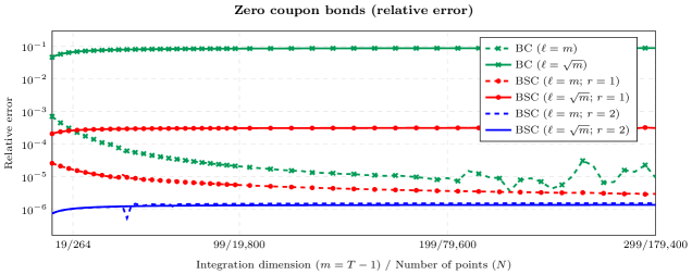
Figure 2: Numerical computation of the integral (26) using fully symmetric Bayesian cubature (BC) and Bayes–Sard cubature (BSC) for different choices of the length-scale $\ell$ and polynomial degree $r$ of the parameteric function space $\pi$ used in BSC.

The choice of generator vectors $\Lambda=\{\boldsymbol{\lambda}^{1},\ldots,\boldsymbol{\lambda}^{J}\}$ for a fully symmetric point set is practically important and has not yet been discussed. In principle one may wish to select $\Lambda$ in order to minimise a criterion, such as the posterior standard deviation $\sigma_{N}$. However, it appears that such optimal $\Lambda$ are mathematically intractable in general. Moreover, numerical optimisation methods cannot be naively applied to approximate the optimal $\Lambda$, since in high dimensions a sparsity structure in the generator vectors $\boldsymbol{\lambda}^{j}$ is required to prevent creation of massive point sets $[\boldsymbol{\lambda}^{j}]$. Thus, although we cannot provide definitive guidelines on how to select the generators in the setting of this article, there are some useful heuristics that have guided us in the examples to follow and those presented in (Karvonen2018, , Section 5):

• In low dimensions, say $m\leq 4$, it is feasible to use (quasi) Monte Carlo samples as generators, as each fully symmetric set will contain at most $384$ points (see Table 1). However, a large number of fully symmetric sets may be needed to ensure sufficient coverage of the space. This approach can work, as in Section 6.3, but is occasionally prone to failure (Karvonen2018, , Section 5.3).

• In higher dimensions (or when a more robust design is desired), we recommend selecting a tried-and-tested fully symmetric point set, such as a sparse grid (Holtz2011, , Chapter 4). This can then be further modified if required, since fully symmetric sets can be added or removed at will. In very high dimensions, this can amount to using effectively low-dimensional generator vectors of the forms $(x_{1},0,\ldots,0)$, $(x_{2},0,\ldots,0)$, $(x_{1},x_{2},0,\ldots,0)$ and so on, for points $x_{i}$ that come from some classical one-dimensional integration rule, such as Gauss–Hermite or Clenshaw–Curtis.

These principles guided our choice of fully symmetric point sets in the sequel.

6.2 Zero Coupon Bonds

This example involves a model for zero coupon bonds that has been used to assess accuracy and robustness of the Bayes–Sard cubature and fully symmetric Bayesian cubature methods in Karvonen2018 ; Karvonen2018c .

6.2.1 Integration Problem

The integral of interest, arising from Euler–Maruyama discretisation of the Vasicek model, is

$$\begin{split}P(0,T)&\coloneqq\mathbb{E}\Bigg{[}\exp\bigg{(}-\Delta t\sum_{i=0}^{T-1}r_{t_{i}}\bigg{)}\Bigg{]}\\ &=\exp(-\Delta tr_{t_{0}})\mathbb{E}\Bigg{[}\exp\bigg{(}-\Delta t\sum_{i=1}^{T-1}r_{t_{i}}\bigg{)}\Bigg{]},\end{split}$$ (26)

where $r_{t_{i}}$ are particular Gaussian random variables and $\Delta t$ and $r_{t_{0}}$ are parameters of the integrand. The dimension $m=T-1$ of the integrand can be freely selected and the integral admits a convenient closed-form solution; see (Holtz2011, , Section 6.1) or (Karvonen2018, , Section 5.5) for a more complete description of this benchmark integral.

6.2.2 Setting

The accuracy of the standard Bayesian cubature and Bayes–Sard cubature methods was compared, for computing the integral (26) in a setting identical to that of (Karvonen2018, , Section 5.5). In particular, the same parameter values and point set (a sparse grid based on a certain Gauss–Hermite sequence with the origin removed), were used. The kernel was the Gaussian kernel with length-scale $\ell>0$:

$$k(\boldsymbol{x},\boldsymbol{x}^{\prime})=\exp\bigg{(}\!-\frac{\mathinner{\lVert\boldsymbol{x}-\boldsymbol{x}^{\prime}\rVert}^{2}}{2\ell^{2}}\bigg{)}.$$ (27)

Accuracy of the two cubature methods was assessed for the heuristic length-scale choices $\ell=m$ and $\ell=\sqrt{m}$. The linear space $\pi$ in the Bayes–Sard method, defined by the collection $\pi_{\alpha}$ of multi-indices, was taken to be $\pi_{\alpha}=\{\boldsymbol{\alpha}\mathrel{\mathop{\ordinarycolon}}|\alpha|\leq r\}$ for either $r$ = 1 (linear) or $r=2$ (quadratic) polynomials. The dimension $T$ ranged between 20 and 300. Since the number of points in a sparse grid depends on the dimension, the maximal $N$ used was $179,\!400$. Theorems 2.1 and 3.1 facilitated the computation, respectively, of the standard Bayesian cubature and Bayes–Sard cubature method. Note that, in the results that are presented next, even though $N$ increases, no convergence (or necessarily monotonicity of the error) is to be expected because the integration problem becomes more difficult as $T$ is increased.

6.2.3 Results

The results are depicted in Figure 2. We observe that Bayes–Sard method is much less sensitive to the length-scale choice compared to the standard Bayesian cubature method. For instance, the selection $\ell=\sqrt{m}$ has Bayes–Sard outperform the standard Bayesian cubature by roughly three orders of magnitude. It is also clear that, in this particular problem, the addition of more polynomial basis functions can significantly improve the integral estimates.

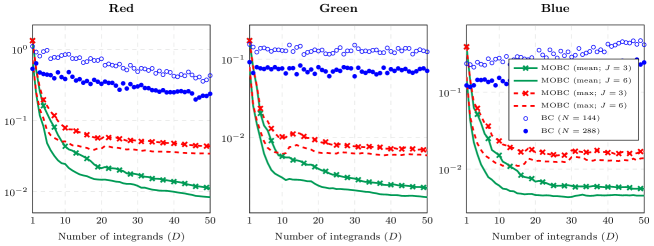
Figure 3: The mean (green; Equation (29)) and maximal (red; Equation (30)) relative integration errors obtained when simultaneously approximating $D$ global illumination integrals (28) using Bayesian cubature (BC) with random points and fully symmetric multi-output Bayesian cubature (MOBC). Here $J=3$ and $J=6$ random generator vectors were used to produce a fully symmetric point set of size $N=144$ (for $J=3$) and $N=288$ (for $J=6$). The displayed results have been averaged over 100 independent realisations of the point sets.

Results at this scale were not possible to obtain in the earlier work of Karvonen et al. Karvonen2018c , where the largest value of $N$ considered was 5,000. In contrast, our result in Theorem 3.1 enabled point sets of size up to ${N=179,\!400}$ to be used. The computational time required to produce the the results for the Bayes–Sard cubature in the most demanding case, $T=300$ and ${m=2}$, was on the order of 2.5 minutes on a standard laptop computer. However, this can be mostly attributed to a sub-optimal algorithm for generating the sparse grid. Indeed, after the points had been obtained it took roughly one second to compute the Bayes–Sard weights.

6.3 Global Illumination Integrals

Next we considered the multi-output Bayesian cubature method, together with the symmetry exploit developed in Section 4.1, to compute a collection of closely related integrals arising in a global illumination context. This is a popular application of Bayesian cubature methods; see Brouillat2009 ; Marques2013 ; Marques2015 ; Briol2017 ; Xi2018 for existing work. In particular, multi-output Bayesian cubature was applied to the problem that we consider below in Xi2018 , where $D=5$ integrals were simultaneously computed. Through computational simplifications obtained by using fully symmetric sets, in what follows we simultaneously compute up to $D=50$ integrals, a ten-fold improvement.

6.3.1 Integration Problem

Global illumination is concerned with the rendering of glossy objects in a virtual environment Dutre2006 . The integration problem studied here is to compute the outgoing radiance $L_{0}(\boldsymbol{\omega}_{o})$ in the direction $\boldsymbol{\omega}_{o}$, for different values of the observation angle $\boldsymbol{\omega}_{o}$. In practical terms, this represents the amount of light travelling from the object to an observer at an observation angle $\boldsymbol{\omega}_{o}$. The need for simultaneous computation for different $\boldsymbol{\omega}_{o}$ can arise when the observation angle is rapidly changing, for example as the player moves in a video game context. The outgoing radiance is given by the integral

$$L_{0}(\boldsymbol{\omega}_{0})=L_{e}(\boldsymbol{\omega}_{0})+\int_{\mathbb{S}^{2}}L_{i}(\boldsymbol{\omega}_{i})\rho(\boldsymbol{\omega}_{i},\boldsymbol{\omega}_{o})[\boldsymbol{\omega}_{i}^{\textsf{T}}\boldsymbol{n}]_{+}\operatorname{d\!}\nu(\boldsymbol{\omega}_{i})$$

with respect to the uniform (i.e. Riemannian) measure $\nu$ on the unit sphere

$$\mathbb{S}^{2}=\big{\{}\boldsymbol{x}\in\mathbb{R}^{3}\>\colon\mathinner{\lVert\boldsymbol{x}\rVert}=1\big{\}}\subset\mathbb{R}^{3}.$$

Here $L_{e}(\boldsymbol{\omega}_{o})$ is the amount of light emitted by the object itself, essentially a constant, whilst $L_{i}(\boldsymbol{\omega}_{i})$ is the amount of light being reflected from the object, originating from angle $\boldsymbol{\omega}_{i}\in\mathbb{S}^{2}$. That reflection is impossible from a reflexive angle is captured by the term $[\boldsymbol{\omega}_{i}^{\textsf{T}}\boldsymbol{n}]_{+}\coloneqq\max\{0,\boldsymbol{\omega}_{i}^{\textsf{T}}\boldsymbol{n}\}$ with $\boldsymbol{n}$ the unit normal to the object. That light is reflected less efficiently at larger incidence angles is captured by a bidirectional reflectance distribution function

$$\rho(\boldsymbol{\omega}_{i},\boldsymbol{\omega}_{o})=\frac{1}{2\pi}\exp\big{(}\boldsymbol{\omega}_{i}^{\textsf{T}}\boldsymbol{\omega}_{o}-1\big{)}.$$

Evaluation of $L_{i}(\boldsymbol{\omega}_{i})$ involves a call to an environment map (in this case, a picture of a lake in California; see Briol2017 ), which is associated with a computational communication cost. The illumination integral must be computed for each of the red, green, and blue (RGB) colour channels; we treat the integration problems corresponding to different colour channels as statistically independent.

6.3.2 Setting

The performance of the standard Bayesian cubature and multi-output Bayesian cubature methods was assessed on a collection of $D$ related integrals, where $D$ was varied up to a maximum of $D_{\text{max}}=50$. The integrands were indexed by observation angles $\boldsymbol{\omega}_{o}^{d}$ with a fixed azimuth and elevation ranging uniformly on the interval $[\frac{\pi}{4}-\frac{\pi}{24},\frac{\pi}{4}+\frac{\pi}{24}]$:

$$\boldsymbol{\omega}_{o}^{d}\mathrel{\mathop{\ordinarycolon}}=\Bigg{(}0,\frac{\pi}{4}-\frac{\pi}{24}\bigg{[}1-2\left(\frac{d-1}{D_{\text{max}}-1}\right)\bigg{]}\Bigg{)}.$$

To formulate the problem in the multi-output framework, we define the associated integrands

$$f^{\dagger}_{d}=L_{i}(\boldsymbol{\omega}_{i})\rho(\boldsymbol{\omega}_{i},\boldsymbol{\omega}_{o}^{d})[\boldsymbol{\omega}_{i}^{\textsf{T}}\boldsymbol{n}]_{+}$$

for $d=1,\ldots,D_{\text{max}}$. The aim is then to compute the integrals

$$I(f^{\dagger}_{d})\coloneqq\int_{\mathbb{S}^{2}}f^{\dagger}_{d}(\boldsymbol{\omega}_{i})\operatorname{d\!}\nu(\boldsymbol{\omega}_{i}).$$ (28)

In our experiments a separable vector-valued covariance function was used, defined as in (22) with

$$c(\boldsymbol{x},\boldsymbol{x}^{\prime})=\frac{8}{3}-\mathinner{\lVert\boldsymbol{x}-\boldsymbol{x}^{\prime}\rVert},\qquad[\boldsymbol{B}]_{dq}=\exp\big{(}(\boldsymbol{\omega}_{o}^{d})^{\textsf{T}}\boldsymbol{\omega}_{o}^{q}-1\big{)}.$$

This prior structure is identical to that used in Briol2017 ; Xi2018 and corresponds to assuming that the integrand belongs to a Sobolev space of smoothness $\frac{3}{2}$. The kernel $c$ has tractable kernel means: $c_{\nu}(\boldsymbol{x})=\frac{4}{3}$ for every $\boldsymbol{x}\in\mathbb{S}^{2}$ and $c_{\nu,\nu}=\frac{4}{3}$.

In order to exploit Theorems 2.1 and 4.1, we need to restrict to fully symmetric point sets on $\mathbb{S}^{2}$. To obtain such sets we followed the method proposed in (Karvonen2018, , Section 5.3). That is, we draw, for each $d=1,\ldots,D$, either $J=3$ or $J=6$ independent generator vectors from the uniform distribution $\nu$ on $\mathbb{S}^{2}$ and use these to generate distinct fully symmetric point sets $X_{1},\ldots,X_{D_{\text{max}}}\subset\mathbb{S}^{2}$. Equation (9) implies that $N=3\times 48=144$ or $N=6\times 48=288$. This approach to generation of a point set was selected for its simplicity, our main focus being on the multi-output framework and a large number of integrals $D$. Alternative point sets on $\mathbb{S}^{2}$ are numerous, such as rotated adaptations of numerically computed approximations to the optimal quasi Monte Carlo designs developed in Brauchart2014 .

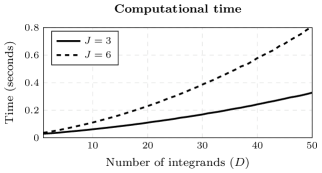
Figure 4: Average computational time (over 100 independent runs), integrand evaluations included, for computation of the fully symmetric multi-output Bayesian cubature estimates for one color channel. The algorithm was implemented in MATLAB and run on a desktop computer with an Intel Xeon 3.40 GHz processor and 15 GB of RAM.

6.3.3 Results

The results are depicted in Figure 3 in terms of the relative integration error for each RGB colour channel. For ${D=1,\ldots,D_{\text{max}}}$, define the vector-valued functions

$$\boldsymbol{f}^{\dagger,D}=(f^{\dagger}_{1},\ldots,f^{\dagger}_{D})\colon\mathbb{S}^{2}\to\mathbb{R}^{D}.$$

The figure shows the improvement in integration accuracy when $D$ increases and more integrands are considered simultaneously. Displayed are the mean

$$\frac{1}{D}\sum_{d=1}^{D}\frac{\mathinner{\!\bigl{\lvert}I(f^{\dagger}_{d})-[\boldsymbol{\mu}_{N}(\boldsymbol{f}^{\dagger,D})]_{d}\bigr{\rvert}}}{I(f^{\dagger}_{d})}$$ (29)

and maximal

$$\max_{d=1,\ldots,D}\frac{\mathinner{\!\bigl{\lvert}I(f^{\dagger}_{d})-[\boldsymbol{\mu}_{N}(\boldsymbol{f}^{\dagger,D})]_{d}\bigr{\rvert}}}{I(f^{\dagger}_{d})}$$ (30)

relative errors for $D=1,\ldots,D_{\text{max}}$. For comparison, the figure also contains results for the standard Bayesian cubature method, applied separately to each of the uni-output integrands $f^{\dagger}_{d}$. Each of the reference integrals $I(f^{\dagger}_{d})$ was computed using brute force Monte Carlo, with 10 million points used.

In accordance with Xi2018 , we observed that the multi-output Bayesian cubature method is superior to the standard one already when $D=5$. The performance gain of the multi-output method keeps increasing when more integrands are added but is ultimately bounded. This is reasonable since integrands for wildly different $\boldsymbol{\omega}_{o}^{d}$ can convey little information about each other. For the smallest values of $D$ the multi-output method is less accurate than the standard Bayesian cubature method. This can be explained by potential non-uniform covering of the unit sphere when the total number $DJ$ of fully symmetric sets is low (e.g., when some of the generator vectors happen to cluster, the fully symmetric sets they generated do not greatly differ, so that less information is obtained on the integrand). For instance, the standard deviation over the 100 runs in the relative error of fully symmetric Bayesian cubature for the first integral (i.e., the case $D=1$ in Figure 3) was 0.34 ($J=3$) or 0.17 ($J=6$) while that of the standard Bayesian cubature with random points was only 0.19 ($N=144$) or 0.11 ($N=288$). See also (Karvonen2018, , Figure 5.1).

Computational times remained reasonable throughout this experiment; see Figure 4. For example, without symmetry exploits, the case $D=50$ and $J=6$ would require $(DN)^{2}=$ 207,360,000 kernel evaluations and inversion of a 14,400-dimensional matrix while Theorem 4.1 reduces these numbers, respectively, to ${DNJ=86,\!400}$ and $DJ=300$. From Figure 4 it is seen that this computation took only 0.8 seconds. This suggests that with more carefully selected fully symmetric point sets it may be possible to realise the desire expressed in (Xi2018, , Section 4) of simultaneous computation of up to thousands of related integrals.

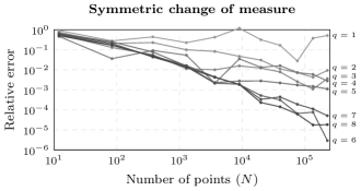
Figure 5: Relative error in numerical integration of the function (31) using the fully symmetric Bayesian cubature method based on a symmetric change of measure. Here $q$ is used to index symmetricity of $\nu$ and thus more challenging $\nu$ correspond to small $q$.

6.4 Symmetric Change of Measure Illustration

The purpose of this final experiment is to briefly illustrate the symmetric change of measure technique, proposed in Section 5. To limit scope we consider applying this technique in conjunction with the fully symmetric standard Bayesian cubature method (i.e., Theorem 2.1).

6.4.1 Integration Problem

Let $\boldsymbol{\mu}_{f}\in\mathbb{R}^{6}$ and $\boldsymbol{\Sigma}_{f}\in\mathbb{R}^{6\times 6}$ be a vector and a positive-definite matrix. Consider integration over $\mathbb{R}^{6}$ of the function

$$f^{\dagger}(\boldsymbol{x})=\exp\bigg{(}\!-\frac{1}{2}(\boldsymbol{x}-\boldsymbol{\mu}_{f})^{\textsf{T}}\boldsymbol{\Sigma}_{f}^{-1}(\boldsymbol{x}-\boldsymbol{\mu}_{f})\bigg{)}$$ (31)

with respect to a Gaussian mixture distribution, $\nu$, to be specified. Integrals of this form can be easily computed in closed form. For this illustration we took

$$\boldsymbol{\mu}_{f}=\begin{bmatrix}\frac{1}{5}\\ \frac{1}{5}+\frac{3}{50}\\ \vdots\\ \frac{1}{2}-\frac{3}{50}\\ \frac{1}{2}\end{bmatrix},\quad\boldsymbol{\Sigma}_{f}=\begin{bmatrix}\big{(}\frac{4}{5}\big{)}^{2}\boldsymbol{I}_{3}&\boldsymbol{0}_{3\times 3}\\ \boldsymbol{0}_{3\times 3}&\big{(}\frac{11}{10}\big{)}^{2}\boldsymbol{I}_{3}\end{bmatrix}.$$

6.4.2 Setting

For these experiments $\nu$ was taken to be a uniform mixture of eight Gaussian distributions $\mathrm{N}(\boldsymbol{\mu}_{i},\boldsymbol{\Sigma}_{i})$, ${i=1,\dots,8}$, with their mean vectors drawn independently from the standard normal distributions and detrended so that $\sum_{i=1}^{8}\boldsymbol{\mu}_{i}=\boldsymbol{0}$. The covariance matrices of each Gaussian component were independent and normalised draws from the Wishart distribution $W_{6}(\boldsymbol{I}_{6},d+2(q-1))$, $q\in\mathbb{N}$. The resulting $\nu$ is almost surely not fully symmetric and therefore Theorem 2.1 cannot be applied. Different values of $q$ correspond to different degrees of symmetricity of $\nu$: for small values of $q$ covariance matrices $\boldsymbol{\Sigma}_{i}$ are likely to be nearly singular, while as $q\to\infty$ they become diagonal. Accordingly, we experimented with $q\in\{1,\ldots,8\}$. For each $q$, the proposal distribution $\nu_{*}$ was a zero-mean Gaussian with diagonal covariance $\sigma^{2}\boldsymbol{I}_{6}$ for $\sigma^{2}$ set to the mean of the diagonal elements of the $\boldsymbol{\Sigma}_{i}$. For Bayesian cubature we used the Gaussian kernel (27) with a length-scale $\ell=0.8$ and the Gauss–Hermite sparse grid (Karvonen2018, , Section 4.2) with the mid-point removed. Note that the resulting point sets are not nested for different $N$.

6.4.3 Results

The results of are depicted in Figure 5 for one fairly representative run. Note how larger values of $q$ correspond to improved integration accuracy. It appears that for reasonably symmetric constituent distributions the proposed method works well; when the covariance matrices are nearly singular we have observed that this simple procedure can seriously fail. This is analogous to scenarious where standard importance sampling can be expected to fare well Robert2013 . Thus, based on this example at least, the symmetric change of measure technique appears to be a promising strategy to generalise the results in Theorems 2.1, 3.1 and 4.1. The largest point sets considered contained $J=168$ fully symmetric sets, which correspond to a point set of size $N=227,\!304$.

7 Discussion

There is increasing interest in the use of Bayesian methods for numerical integration Briol2017 . Bayesian cubature methods are attractive due to analytic and theoretical tractability of the underlying Gaussian model. However, these method are also associated with a computational cost that is cubic in the number of points, $N$, and moreover the linear systems that must be inverted are typically ill-conditioned.

The symmetry exploits developed in this work circumvent the need for large linear systems to be solved in Bayesian cubature methods. In particular, we presented novel results for Bayes–Sard cubature Karvonen2018c and multi-output Bayesian cubature Xi2018 that make it possible to apply these methods even for extremely large datasets or when there are many function to be integrated. In conjunction with the inherent robustness of the Bayes–Sard cubature method Karvonen2018c , this results in a highly reliable probabilistic integration method that can be applied even to integrals that are relatively high-dimensional.

Three extensions of this work are highlighted: First, the combination of multi-output and Bayes–Sard methods appears to be a natural extension and we expect that symmetry properties can similarly be exploited for this method. This could lead to promising procedures for integration of collections of closely related high-dimensional functions appearing in, for example, financial applications Holtz2011 . Similarly, our exploits should extend to the Student’s $t$ based Bayesian cubatures proposed in Prueher2017 . Second, the investigation of optimality criteria for the symmetric change of measure technique in Section 5 remains to be explored. Third, although we focussed solely on computational aspects, the important statistical question of how to ensure Bayesian cubature methods produce output that is well-calibrated remains to some extent unresolved. As discussed in Karvonen2018 , it appears that symmetry exploits do not easily lend themselves to selection of kernel parameters, for instance via cross-validation or maximisation of marginal likelihood. A potential, though somewhat heuristic, way to proceed might be to exploit the concentration of measure phenomenon Ledoux2001 or low effective dimensionality of the integrand WangSloan2005 in order to identify a suitable data subset on which kernel parameters can be calibrated more easily or a priori.

- (1) Bach, F.: On the equivalence between kernel quadrature rules and random feature expansions. Journal of Machine Learning Research 18(21), 1–38 (2017). URL http://www.jmlr.org/papers/volume18/15-178/15-178.pdf
- (2) Bach, F., Lacoste-Julien, S., Obozinski, G.: On the equivalence between herding and conditional gradient algorithms. In: Proceedings of the 29th International Conference on Machine Learning, pp. 1355–1362 (2012). URL https://icml.cc/2012/papers/683.pdf
- (3) Berlinet, A., Thomas-Agnan, C.: Reproducing Kernel Hilbert Spaces in Probability and Statistics. Springer Science & Business Media (2011)
- (4) Bezhaev, A.Yu.: Cubature formulae on scattered meshes. Soviet Journal of Numerical Analysis and Mathematical Modelling 6(2), 95–106 (1991). DOI 10.1515/rnam.1991.6.2.95
- (5) Brauchart, J.S., Saff, E.B., Sloan, I.H., Womersley, R.S.: QMC designs: Optimal order quasi Monte Carlo integration schemes on the sphere. Mathematics of Computation 83(290), 2821–2851 (2014). DOI 10.1090/S0025-5718-2014-02839-1
- (6) Briol, F.X., Oates, C.J., Cockayne, J., Chen, W.Y., Girolami, M.: On the sampling problem for kernel quadrature. In: Proceedings of the 34th International Conference on Machine Learning, pp. 586–595 (2017). URL http://proceedings.mlr.press/v70/briol17a.html
- (7) Briol, F.X., Oates, C.J., Girolami, M., Osborne, M.A.: Frank-Wolfe Bayesian quadrature: Probabilistic integration with theoretical guarantees. In: Advances in Neural Information Processing Systems, vol. 28, pp. 1162–1170 (2015). URL https://papers.nips.cc/paper/5749-frank-wolfe-bayesian-quadrature-probabilistic-integration-with-theoretical-guarantees
- (8) Briol, F.X., Oates, C.J., Girolami, M., Osborne, M.A., Sejdinovic, D.: Probabilistic integration: A role in statistical computation? (with discussion). Statistical Science (2018). URL https://arxiv.org/abs/1512.00933. To appear.
- (9) Brouillat, J., Bouville, C., Loos, B., Hansen, C., Bouatouch, K.: A Bayesian Monte Carlo approach to global illumination. Computer Graphics Forum 28(8), 2315–2329 (2009). DOI 10.1111/j.1467-8659.2009.01537.x
- (10) Chai, H., Garnett, R.: An improved Bayesian framework for quadrature of constrained integrands (2018). URL https://arxiv.org/abs/1802.04782
- (11) Chen, W., Mackey, L., Gorham, J., Briol, F.X., Oates, C.J.: Stein points. In: Proceedings of the 35th International Conference on Machine Learning (2018). URL http://proceedings.mlr.press/v80/chen18f
- (12) Cockayne, J., Oates, C.J., Sullivan, T., Girolami, M.: Bayesian probabilistic numerical methods (2017). URL https://arxiv.org/abs/1702.03673
- (13) Cools, R.: Constructing cubature formulae: the science behind the art. Acta Numerica 6, 1–54 (1997). DOI 10.1017/S0962492900002701
- (14) Davis, P.J., Rabinowitz, P.: Methods of Numerical Integration. Courier Corporation (2007)
- (15) DeVore, R., Foucart, S., Petrova, G., Wojtaszczyk, P.: Computing a quantity of interest from observational data. Constructive Approximation (2018). DOI 10.1007/s00365-018-9433-7. To appear
- (16) Diaconis, P.: Bayesian numerical analysis. In: Statistical Decision Theory and Related Topics IV, vol. 1, pp. 163–175. Springer-Verlag New York (1988). DOI 10.1007/978-1-4613-8768-8˙20
- (17) Dietrich, C.R., Newsam, G.N.: Fast and exact simulation of stationary gaussian processes through circulant embedding of the covariance matrix. SIAM Journal on Scientific Computing 18(4), 1088–1107 (1997). DOI 10.1137/s1064827592240555
- (18) Dutre, P., Bekaert, P., Bala, K.: Advanced global illumination. AK Peters/CRC Press (2006). DOI 10.1201/9781315365473
- (19) Ehler, M., Graef, M., Oates, C.J.: Optimal Monte Carlo integration on closed manifolds. Statistics and Computing (2019). URL https://arxiv.org/abs/1707.04723. To appear
- (20) Genz, A.: Fully symmetric interpolatory rules for multiple integrals. SIAM Journal on Numerical Analysis 23(6), 1273–1283 (1986). DOI 10.1137/0723086
- (21) Genz, A., Keister, B.D.: Fully symmetric interpolatory rules for multiple integrals over infinite regions with Gaussian weight. Journal of Computational and Applied Mathematics 71(2), 299–309 (1996). DOI 10.1016/0377-0427(95)00232-4
- (22) Gunter, T., Osborne, M.A., Garnett, R., Hennig, P., Roberts, S.J.: Sampling for inference in probabilistic models with fast Bayesian quadrature. In: Advances in Neural Information Processing Systems, vol. 27, pp. 2789–2797 (2014). URL https://papers.nips.cc/paper/5483-sampling-for-inference-in-probabilistic-models-with-fast-bayesian-quadrature
- (23) Hackbusch, W.: A sparse matrix arithmetic based on -matrices. part I: Introduction to -matrices. Computing 62(2), 89–108 (1999). DOI 10.1007/s006070050015
- (24) Hennig, P., Osborne, M.A., Girolami, M.: Probabilistic numerics and uncertainty in computations. Proceedings of the Royal Society of London A: Mathematical, Physical and Engineering Sciences 471(2179) (2015). DOI 10.1098/rspa.2015.0142
- (25) Hensman, J., Durrande, N., Solin, A.: Variational Fourier features for Gaussian processes. Journal of Machine Learning Research 11(151), 1–52 (2018). URL https://www.jmlr.org/papers/volume18/16-579/16-579.pdf
- (26) Holtz, M.: Sparse Grid Quadrature in High Dimensions with Applications in Finance and Insurance. No. 77 in Lecture Notes in Computational Science and Engineering. Springer (2011). DOI 10.1007/978-3-642-16004-2
- (27) Jagadeeswaran, R., Hickernell, F.J.: Fast automatic Bayesian cubature using lattice sampling (2018). URL https://arxiv.org/abs/1809.09803. Submitted
- (28) Kanagawa, M., Sriperumbudur, B.K., Fukumizu, K.: Convergence guarantees for kernel-based quadrature rules in misspecified settings. In: Advances in Neural Information Processing Systems, vol. 29, pp. 3288–3296 (2016). URL https://arxiv.org/abs/1605.07254
- (29) Kanagawa, M., Sriperumbudur, B.K., Fukumizu, K.: Convergence analysis of deterministic kernel-based quadrature rules in misspecified settings. Foundations of Computational Mathematics (2019). DOI 10.1007/s10208-018-09407-7. To appear
- (30) Karvonen, T., Särkkä, S.: Classical quadrature rules via Gaussian processes. In: 27th IEEE International Workshop on Machine Learning for Signal Processing (2017). DOI 10.1109/mlsp.2017.8168195
- (31) Karvonen, T., Särkkä, S.: Fully symmetric kernel quadrature. SIAM Journal on Scientific Computing 40(2), A697–A720 (2018). DOI 10.1137/17m1121779
- (32) Karvonen, T., Särkkä, S., Oates, C.J.: A Bayes–Sard cubature method. In: Advances in Neural Information Processing Systems, vol. 31 (2018). URL https://papers.nips.cc/paper/7829-a-bayes-sard-cubature-method. To appear
- (33) Kennedy, M.: Bayesian quadrature with non-normal approximating functions. Statistics and Computing 8(4), 365–375 (1998). DOI 10.1023/A:1008832824006
- (34) Larkin, F.M.: Gaussian measure in Hilbert space and applications in numerical analysis. The Rocky Mountain Journal of Mathematics 2(3), 379–421 (1972). DOI 10.1216/rmj-1972-2-3-379
- (35) Larkin, F.M.: Probabilistic error estimates in spline interpolation and quadrature. In: Information Processing 74 (Proceedings of IFIP Congress, Stockholm, 1974), vol. 74, pp. 605–609. North-Holland (1974)
- (36) Lázaro-Gredilla, M., Quiñonero-Candela, J., Rasmussen, C.E., Figueiras-Vidal, A.R.: Sparse spectrum Gaussian process regression. Journal of Machine Learning Research 11, 1865–1881 (2010). URL http://jmlr.csail.mit.edu/papers/v11/lazaro-gredilla10a.html
- (37) Ledoux, M.: The Concentration of Measure Phenomenon. No. 89 in Mathematical Surveys and Monographs. American Mathematical Society (2001). DOI 10.1090/surv/089
- (38) Lu, J., Darmofal, D.L.: Higher-dimensional integration with Gaussian weight for applications in probabilistic design. SIAM Journal on Scientific Computing 26(2), 613–624 (2004). DOI 10.1137/s1064827503426863
- (39) Marques, R., Bouville, C., Ribardière, M., Santos, L.P., Bouatouch, K.: A spherical Gaussian framework for Bayesian Monte Carlo rendering of glossy surfaces. IEEE Transactions on Visualization and Computer Graphics 19(10), 1619–1932 (2013). DOI 10.1109/tvcg.2013.79
- (40) Marques, R., Bouville, C., Santos, L.P., Bouatouch, K.: Efficient Quadrature Rules for Illumination Integrals: from Quasi Monte Carlo to Bayesian Monte Carlo. Synthesis Lectures on Computer Graphics and Animation. Morgan & Claypool Publishers (2015). DOI 10.2200/s00649ed1v01y201505cgr019
- (41) McNamee, J., Stenger, F.: Construction of fully symmetric numerical integration formulas. Numerische Mathematik 10(4), 327–344 (1967). DOI 10.1007/BF02162032
- (42) Minka, T.: Deriving quadrature rules from Gaussian processes. Tech. rep., Microsoft Research, Statistics Department, Carnegie Mellon University (2000). URL https://www.microsoft.com/en-us/research/publication/deriving-quadrature-rules-gaussian-processes/
- (43) Najm, H.N., Debusschere, B.J., Marzouk, Y.M., Widmer, S., Le Maître, O.: Uncertainty quantification in chemical systems. International Journal for Numerical Methods in Engineering 80(6-7), 789–814 (2009). DOI 10.1002/nme.2551
- (44) Novak, E., Ritter, K.: Simple cubature formulas with high polynomial exactness. Constructive Approximation 15(4), 499–522 (1999). DOI 10.1007/s003659900119
- (45) Novak, E., Ritter, K., Schmitt, R., Steinbauer, A.: On an interpolatory method for high dimensional integration. Journal of Computational and Applied Mathematics 112(1–2), 215–228 (1999). DOI 10.1016/s0377-0427(99)00222-8
- (46) Oates, C.J., Niederer, S., Lee, A., Briol, F.X., Girolami, M.: Probabilistic models for integration error in the assessment of functional cardiac models. In: Advances in Neural Information Processing Systems, vol. 30, pp. 109–117 (2017). URL http://papers.nips.cc/paper/6616-probabilistic-models-for-integration-error-in-the-assessment-of-functional-cardiac-models
- (47) Oettershagen, J.: Construction of optimal cubature algorithms with applications to econometrics and uncertainty quantification. Ph.D. thesis, Institut für Numerische Simulation, Universität Bonn (2017)
- (48) O’Hagan, A.: Curve fitting and optimal design for prediction. Journal of the Royal Statistical Society. Series B (Methodological) 40(1), 1–42 (1978). DOI 10.1111/j.2517-6161.1978.tb01643.x
- (49) O’Hagan, A.: Bayes–Hermite quadrature. Journal of Statistical Planning and Inference 29(3), 245–260 (1991). DOI 10.1016/0378-3758(91)90002-v
- (50) Osborne, M., Garnett, R., Ghahramani, Z., Duvenaud, D.K., Roberts, S.J., Rasmussen, C.E.: Active learning of model evidence using Bayesian quadrature. In: Advances in Neural Information Processing Systems, vol. 25, pp. 46–54 (2012). URL https://papers.nips.cc/paper/4657-active-learning-of-model-evidence-using-bayesian-quadrature
- (51) Osborne, M., Garnett, R., Roberts, S., Hart, C., Aigrain, S., Gibson, N.: Bayesian quadrature for ratios. In: Artificial Intelligence and Statistics, pp. 832–840 (2012). URL http://proceedings.mlr.press/v22/osborne12/osborne12.pdf
- (52) Pronzato, L., Zhigljavsky, A.: Bayesian quadrature and energy minimization for space-filling design (2018). URL https://arxiv.org/abs/1808.10722
- (53) Prüher, J., Tronarp, F., Karvonen, T., Särkkä, S., Straka, O.: Student- process quadratures for filtering of non-linear systems with heavy-tailed noise. In: 20th International Conference on Information Fusion (2017). DOI 10.23919/icif.2017.8009742
- (54) Rasmussen, C.E., Williams, C.K.I.: Gaussian Processes for Machine Learning. MIT Press (2006)
- (55) Robert, C., Casella, G.: Monte Carlo Statistical Methods. Springer Science & Business Media (2013)
- (56) Särkkä, S., Hartikainen, J., Svensson, L., Sandblom, F.: On the relation between Gaussian process quadratures and sigma-point methods. Journal of Advances in Information Fusion 11(1), 31–46 (2016). URL https://arxiv.org/abs/1504.05994
- (57) Schaback, R.: Error estimates and condition numbers for radial basis function interpolation. Advances in Computational Mathematics 3(3), 251–264 (1995). DOI 10.1007/bf02432002
- (58) Schäfer, F., Sullivan, T.J., Owhadi, H.: Compression, inversion, and approximate PCA of dense kernel matrices at near-linear computational complexity (2017). URL https://arxiv.org/abs/1706.02205
- (59) Smola, A., Gretton, A., Song, L., Schölkopf, B.: A Hilbert space embedding for distributions. In: International Conference on Algorithmic Learning Theory, pp. 13–31. Springer (2007). DOI 10.1007/978-3-540-75225-7˙5
- (60) Sommariva, A., Vianello, M.: Numerical cubature on scattered data by radial basis functions. Computing 76(3–4), 295–310 (2006). DOI 10.1007/s00607-005-0142-2
- (61) Stein, M.L.: Interpolation of Spatial Data: Some Theory for Kriging. Springer Science & Business Media (2012)
- (62) Wang, X., Sloan, I.H.: Why are high-dimensional finance problems often of low effective dimension? SIAM Journal on Scientific Computing 27(1), 159–183 (2005). DOI 10.1137/s1064827503429429
- (63) Wendland, H.: Scattered Data Approximation. No. 28 in Cambridge Monographs on Applied and Computational Mathematics. Cambridge University Press (2005)
- (64) Xi, X., Briol, F.X., Girolami, M.: Bayesian quadrature for multiple related integrals. Proceedings of the 35th International Conference on Machine Learning (2018). URL https://arxiv.org/abs/1801.04153. To appear
- (65) Xiu, D., Karniadakis, G.E.: Modeling uncertainty in flow simulations via generalized polynomial chaos. Journal of Computational Physics 187(1), 137–167 (2003). DOI 10.1016/s0021-9991(03)00092-5
- (66) Álvarez, M., Rosasco, L., Lawrence, N.: Kernels for vector-valued functions: A review. Foundations and Trends®in Machine Learning 4(3), 195–266 (2012). DOI 10.1561/2200000036