Fundamentals and model of resonance helicity (RHELT) and energy (RET) transfer between two magnetoelectric chiral particles

Abstract

We establish a classical electrodynamic theory for the non-radiative transfer of field helicity (RHELT) and energy (RET) between a donor and an acceptor, both being dipolar, magnetoelectric and bi-isotropic, chiral in particular, with rotating excited dipoles. We introduce orientational factors that control this process. Also, a RHELT and RET interaction radius is put forward. The detection of RHELT adds a wealth of information contained in the helicity of the transferred fields, never used or established to date. The nature of these dipolar magnetoelectric bi-isotropic particles and/or molecules with induced dipoles possessing angular momentum, enriches the number of variables and associated effects. Hence the landscape involved in this transfer phenomenon, never explored before, is significantly broader than in conventional FRET. In this way, chiral interacting objects convey terms in the equations of transfer rate of helicity and energy that are discriminatory, so that one can extract information on their structural chirality handedness and polarization rotation. As such, not only the rate of electromagnetic helicity transfer, but also that of energy transfer may be negative, which for the latter means an enhanced emission from the donor in pressence of acceptor, a phenomenon which does not exist in conventional FRET. Importantly, both the RHELT and RET rates, as well as the RHELT interaction radius, are very sensitive to changes in the helicity, or state of polarization, of the illumination, as well as to the polarization of the excited electric and magnetic dipole moments of donor and acceptor. Finally, we introduce the observable quanties in terms of which one can obtain the transfer rates and interaction radii.

I Introduction

Electromagnetic wavefields with rotation of their polarization vectors and wavefronts allen1 ; andrews1 ; yao are subjects of increasing interest for their larger number of degrees of freedom as communication channels andrews2 ; boyd , and for providing new capibilities to probing and manipulating both chiral and achiral structures at the micro and nanoscale in light-matter interactions schellman ; richard ; vuong ; bliokh1 ; schukov1 ; brasse ; bliokh2 . In this latter respect, the interplay between the structural symmetry of the light probe and that of matter andrews3 ; nieto1 ; bliokh3 ; kivshar is of upmost importance, since the latter governs the metabolism of living organisms and is becoming of increasing relevance for nanophotonic devices. Nevertheless, our knowledge in this regard is yet incomplete; therefore new probe techniques for chiral nanostructures with rotating dipoles (and multipoles) are still necessary.

Progress in characterizing light chirality and its interaction with matter, on the one hand, tang1 ; bliokh4 ; bliokh5 ; cameron1 ; cameron2 ; nieto2 ; nieto3 ; gutsche1 ; gutsche2 ; gutsche3 ; corbato1 ; zambra1 ; gutsche4 , and on designing structured wavefields that enhance the usually weak interaction with chiral molecules and nanoparticles tang2 ; tang3 ; choi ; klimov ; dionne1 ; schafer1 ; giessen1 ; schafer2 ; dionne2 ; carminati ; wang ; hu , has advanced together with methods to increase the energy transfer between nanostructures kivshar ; carminati , like e.g. Förster energy tranfer (FRET) between molecules and/or particles fret1 ; fret2 ; circpollibro1 . Although this latter phenomenon constitutes nowadays an established technique in nanoscience and biology circpolemission ; kagan , and it has a well developed theory fret1 ; clegg ; novotny ; and in spite of theoretical studies on shifts and transfer of energy between two chiral molecules based on their dipole and quadrupole interactions craig1 ; salam1 ; craig2 ; salam2 , aparently and as far as we know, there are not yet techniques based on characterizing helicity states of the detected light in FRET. This involves field helicity transfer between particles and/or molecules, let them be chiral or achiral; but FRET is based on detecting only omnidirectional intensities emitted by the fluorophores, which can be hindered by limitations depending on the molecule nature and environment configuration, and specially by the low signal-to-noise ratio silas .

In previous work nieto2 we established the law ruling the extinction of electromagnetic helicity of a twisted illuminating wavefield on scattering and absorption by a wide sense g-etxarri ; nieto4 (i.e. non-Rayleigh) dipolar bi-isotropic particle, chiral in particular. Also we put forward the helicity enhancement factor nieto3 when the particle is in an inhomogeneous environment madrazo ; garcia . Such a quantity plays a role analogous to that of the Purcell factor for the energy. This extinction law encompasses a variety of new processes involving the helicity of electromagnetic fields which are emitted, absorbed and/or scattered in presence of other objects nieto3 ; gutsche1 ; gutsche2 .

Extending studies to circularly or elliptically polarized dipoles opens a new landscape on interactions of light and matter, in particular between particles. This has applications in new nanophotonic systems and techniques. Specifically, like electromagnetic theory formulates FRET as the extinction (most frequently, the absorption) by the acceptor A of the energy emitted by the donor D, one may ask on the existence of an analogous phenomenon between two dipoles D and A for the wavefield helicity on illumination of D by rotating light, therefore possessing angular momentum which is conveyed to the donor; specifically when D and A are magnetoelectric and bi-isotropic elliptically, or circularly, polarized dipoles. Addressing this question is the main aim of this paper and, as matter of fact, we gave a hint (cf. Eq.(36) of nieto2 ) on employing our helicity extinction formulation in modelling its transfer between two nanoscale magnetoelectric dipolar bodies. The quantities involved in such a kind of phenomenon go beyond those of standard FRET. For instance, we shall put forward the existence of several orientational factors, instead of just one, $\kappa^{2}$, of standard FRET.

Therefore, in this work we establish a classical electromagnetic theory of resonance helicity transfer, (which we shall abridge as RHELT), between two dipolar particles D and A, (by ”particle” we shall mean either a quantum dot, a molecule, a synthesized material polarizable nanoparticle, or a hybrid between both), both being dipolar and magnetoelectric, bi-isotropic, chiral in particular, and located in the near-field (i.e. non-radiative) region of each other. This brings additional information to estimate their relative distance and orientations, as well as to know donor and acceptor constitutive parameters, and their generally elliptic polarization; thus making it possible to characterize them according to their effects on the electromagnetic helicity, both trasferred from D to A, as well as emitted by the acceptor, (in this connection see e.g. nieto2 ; gutsche4 ). Besides, this configuration adapts to illumination and/or emission of twisting light, like in circularly polarized luminescence circpollibro1 ; circpolemission ; kumar .

In parallel to RHELT, we will also study resonance energy transfer (RET) between these dipolar magnetoelectric bi-isotropic (or chiral) rotating donors and acceptors. We shall address time-harmonic fields at optical frequencies; except when we consider the emission and absorption of donors and acceptors over a range of frequencies, a case in which the fields are taken at a generic frequency of their spectrum, and the polarizabilities are given by their effective values, expressed as overlapping integrals of their respective emission and absorption - or extinction - spectra.

Moreover, due to our lack of data on energy and helicity transfer between magnetoelectric rotating chiral particles, and incomplete knowledge on values of their polarizabilities, and given the progress in the last years in devising and building nanoparticles with a large magnetic response to the field of light nietoJOSA ; g-etxarri ; geffrin ; kuznetsov ; staude ; kivshar_reviews , (which leads to phenomena stemming from the interplay between the particle induced electric and magnetic dipoles), we may envisage a near future of both theretical and experimental research leading to techniques with magnetoelectric conjugates of molecules and nanoparticles, (or even of bulky magnetoelectric molecules) with angular momentum gained on illumination with twisted light. Therefore, we shall address rather large rotating magnetoelectric chiral particles with a diameter of a few tens of $nm$, (see e.g. pyramids ; jaque ; dionne ; chinos ), whether they actually are molecules, dielectric or metallic nanoparticles, or conjugates of them both; and hence possessing large magnetic and cross electric-magnetic polarizabilities, besides the electric one. In this way, the interaction distance that our theory yields with these larger particles gets values considerably greater than the typical $5-10nm$ Förster radii of FRET.

Our results will therefore be qualitative as we shall not address specific material parameters beyond certain models of emission and absorption distributions. For both RHELT and RET we obtain transfer rates that include, besides the electric polarizability term like in conventional FRET, additional contributions of both the cross electric-magnetic and the magnetic polarizabilities of the donor and acceptor and that, therefore, depend on their chirality handedness.

However, we shall show that while the structural chirality, and polarization helicity, of the donor dipoles is implicitely contained in its electric and magnetic dipole moments, included in the transfer rate and interaction radii equations, the chirality of the acceptor appears explicitely as its cross electric-magnetic polarizability in some terms of these RHELT and RET equations. As such, these terms are discriminatory, and thus uniquely characterize the symmetry handedness of A.

Our electromagnetic theory is different from the quantum-mechanical one previously established for transfer and shifts of energy between molecules salam1 ; salam2 ; craig1 ; craig2 , as we deal not only with absorption, but also with electromagnetic scattering. Therefore the extinction (rather than just the absorption) of energy and helicity is considered. Namely, these absorbed plus scattered quantities nieto1 ; nieto2 ; nieto3 are addressed in this work. The $r^{-6}$ interdistance dependence is recovered for RET, as well as for RHELT, as a consequence of D and A being assumed dipoles in the near-field of each other.

Also, while in conventional FRET, the axcitation of A by D conveys a decrease in the energy emitted by D, there being an increase in the energy emitted by A, we shall see that for chiral A and D the energy transfer rate may be negative, which will indicate that the donor emission is enhanced, rather than inhibited, in presence of the acceptor; and, hence, the proximity of A increases the spontaneous decay rate of D. However, a negative helicity rate does not necessarily mean an enhancement of helicity extinction in the donor due to the presence of the acceptor, since the extinction of helicity, at difference with that of energy, is expected to have either negative or positive values, even for purely dielectric interacting particles, depending on the sense of rotation of the emited wavefield.

In the following sections we develop the details of these new phenomena. Finally, we shall also introduce the observables linked to these effects, discussing their behavior and their relationships with the main quantities involved in these transfer processes.

II Dipolar excitation of helicity and energy

In standard FRET, a molecule D excited on illumination emits falling to its ground state, and part of this emitted light is absorbed by a molecule A which is in the near-field zone of D. This process requires that the emission spectrum of D and the absorption spectrum of A have a certain overlap fret1 ; clegg ; novotny , so that such a resonance (i.e. non-radiative) transfer of energy from D to A may take place.

As stated in the introduction, we assume A and D being ”particles” in general, by which we mean either quantum dots, synthesized material nanoparticles, molecules, or conjugates of both of them. We address the spatial parts ${\bf E}({\bf r})$ and ${\bf B}({\bf r})$ of the electric and magnetic vectors of time-harmonic electromagnetic fields in their complex representation. [If A and D emit and extinguish, or absorb, light over a range of frequencies, these fields are understood at a generic frequency of their spectrum: ${\bf E}({\bf r},\omega)$ and ${\bf B}({\bf r,\omega})$]. Their interaction in a medium of refractive index $n=\sqrt{\epsilon\mu}$ with a magnetoelectric, bi-isotropic and dipolar ”particle”, is given through its electric, magnetic, and cross electric-magnetic polarizability tensors: $\underline{\bm{\alpha}}_{e}$, $\underline{\bm{\alpha}}_{m}$, $\underline{\bm{\alpha}}_{em}$ and $\underline{\bm{\alpha}}_{me}$ . $k=n\omega/c=2\pi n/\lambda$. Hence, the electric and magnetic dipole moments, ${\bf p}$ and ${\bf m}$, induced in the particle by this field are given by the constitutive relations: ${\bf p}=\underline{\bm{\alpha}}_{e}{\bf E}+\underline{\bm{\alpha}}_{em}{\bf B}$, ${\bf m}=\underline{\bm{\alpha}}_{me}{\bf E}+\underline{\bm{\alpha}}_{m}{\bf B}$.

In this work we shall consider the bi-isotropic particle being chiral reciprocal, so that $\underline{\bm{\alpha}}_{em}=-\underline{\bm{\alpha}}_{me}^{{}^{{\dagger}}}$. The sign ${\dagger}$ standing for conjugate transpose.

Using a Gaussian system of units, the time-averaged (written as $<\cdot>)$ electromagnetic helicity density of the wavefield: $\mathscr{H}({\bf r})=<\mathscr{H}({\bf r})>=\frac{1}{2k}\sqrt{\frac{\epsilon}{\mu}}\mbox{Im}[{\bf E}({\bf r})\cdot{\bf B}^{*}({\bf r})]$ is a conserved quantity fulfilling the continuity equation nieto2 ; bliokh4 : $\nabla\cdot{\cal F}=-\mathscr{P}$, where ${\cal F}$ is the helicity density flow which for these fields coincides with their spin angular momentum nieto2 ; bliokh4 , and $\mathscr{P}$ denotes the conversion of helicity, i.e. its decrease or increase by absorption and/or scattering of the wavefield by the particle nieto2 ; gutsche2 ; gutsche4 . Henceforth, Re and Im stand for real and imaginary part, respectively; and ^∗ denotes complex conjugate. Most optical wavefields can be decomposed into the sum of a field ${\bf E}^{+}({\bf r})$ with all plane wave components being left circularly polarized (LCP), plus a field ${\bf E}^{-}({\bf r})$ whose components are right circularly polarized (RCP), so that the above helicity density may be expressed as nieto1 ; nieto3 : ${\mathscr{H}}({\bf r})=(\epsilon/2k)[|{\bf E}^{+}({\bf r})|^{2}-|{\bf E}^{-}({\bf r})|^{2}]$; while its time-averged energy density reads: $<{w}({\bf r})>=(\epsilon/8\pi)[|{\bf E}^{+}({\bf r})|^{2}+|{\bf E}^{-}({\bf r})|^{2}]$.

With reference to a Cartesian framework $OXYZ$, (cf. Fig. 1), our analysis is based on the extinction of electromagnetic helicity and energy by the electric and magnetic dipoles ${\bf p}_{A}$ and ${\bf m}_{A}$ of the acceptor particle A, placed at a point of position vector ${\bf r}_{A}$, on interaction with the field ${\bf E}_{D}({\bf r}_{A})$, ${\bf B}_{D}({\bf r}_{A})$ emitted by the rotating electric and magnetic dipoles ${\bf p}_{D}$ and ${\bf m}_{D}$, induced on illumination of the donor particle D by generally twisted light, propagating along a main direction defined by the ${\bf s}_{i}$ vector, (see Fig. 1). In its most general form stemming from the optical theorem, this reads for the transfer of energy from D to A:

$${\cal W}^{DA}=\frac{\omega}{2}\mbox{Im}[{\bf p}_{A}\cdot{\bf E}_{D}^{*}({\bf r}_{A})+{\bf m}_{A}\cdot{\bf B}_{D}^{*}({\bf r}_{A})].$$ (1)

Whereas the extinction of electromagnetic helicity - or wavefield chirality nieto1 ; tang1 ; gutsche4 - in A of the emission from D is, according to the helicity optical theorem, (cf. Eq. (36) of nieto2 ):

$${\cal W}_{\mathscr{H}}^{DA}=2\pi c\mbox{Re}\{-\frac{1}{n^{2}}{\bf p}_{A}\cdot{\bf B}_{D}^{*}({\bf r}_{A})+{\bf m}_{A}\cdot{\bf E}_{D}^{*}({\bf r}_{A})\}.$$ (2)

Eq. (2) determines the total transfer of helicity from D to A.

Figure 1: (Color online). A twisted wave, propagating along ${\bf s}_{i}$, incides on a polarizable donor particle D, inducing dipole moments ${\bf p}_{D}$ and ${\bf m}_{D}$ which emit light, inducing dipoles ${\bf p}_{A}$ and ${\bf m}_{A}$ in the acceptor A.

Expressing the vector pointing from D to A as ${\bf r}_{R}=r{\bf s}_{R}$, $r=|{\bf r}_{R}|$, $|{\bf s}_{R}|=1$, $r$ being the distance between the centers of D and A, (see Fig.1), we write the near-fields ${\bf E}_{D}$ and ${\bf B}_{D}$ emitted by D at the center of A at distance $r$ from the center of D: ${\bf r}_{R}={\bf r}_{A}-{\bf r}_{D}$:

$${\bf E}_{D}({\bf r}_{A})=\frac{1}{\epsilon r^{3}}[3({\bf p}_{D}\cdot{\bf s}_{R})-{\bf p}_{D}];\,\,\,\,\,\,\,\,\,$$

$${\bf B}_{D}({\bf r}_{A})=\frac{\mu}{r^{3}}[3({\bf m}_{D}\cdot{\bf s}_{R})-{\bf m}_{D}].\,\,\,\,\,\,\,\,$$ (3)

A weak coupling regime between D and A is assumed, so that there is no scattering feedback between them.

III RHELT and RET between chiral particles

III.1 Bi-isotropic particles

We shall first consider the donor D and acceptor A magnetoelectric and generally bi-isotropic; subsequently we shall particularize them being chiral. We assume the electric and magnetic dipoles induced in A by the wavefields (3) emitted by D, (transition dipoles if A is a molecule), polarized in directions given by the complex unit vectors ${\bf s}_{A}^{p}$ and ${\bf s}_{A}^{m}$, thus presenting orientational photoselection with respect to the illuminating field from D circpollibro1 ; circpolemission :

$${p}_{A\,i}=\alpha_{e}^{A}s_{A\,i}^{p}s_{A\,j}^{p\,*}{E}_{D\,j}+\alpha_{em}^{A}s_{A\,i}^{p}s_{A\,j}^{m\,*}{B}_{D\,j}=p_{A}s_{A\,i}^{p}.\,\,\,\,\,\,\,\,$$

$${m}_{A\,i}=\alpha_{me}^{A}s_{A\,i}^{m}s_{A\,j}^{p\,*}{E}_{D\,j}+\alpha_{m}^{A}s_{A\,i}^{m}s_{A\,j}^{m\,*}{B}_{D\,j}=m_{A}s_{A\,i}^{m}.\,\,\,\,\,\,\,\,$$

$$p_{A}=\alpha_{e}^{A}s_{A\,j}^{p\,*}{E}_{D\,j}+\alpha_{em}^{A}s_{A\,j}^{m\,*}{B}_{D\,j}.\,\,\,\,\,$$

$$m_{A}=\alpha_{me}^{A}s_{A\,j}^{p\,*}{E}_{D\,j}+\alpha_{m}^{A}s_{A\,j}^{m\,*}{B}_{D\,j}.\,\,\,\,(i,j=1,2,3).\,\,\,\,\,\,\,\,$$ (4)

Having used the notation of summing over all repeated indices. If also D were orientationally photoselective, we would consider its electric and magnetic dipoles, induced by an incident field ${\bf E}^{(i)},{\bf B}^{(i)}$, also polarized in directions given by the complex unit vectors ${\bf s}_{D}^{p}$ and ${\bf s}_{D}^{m}$ as:

$${p}_{D\,i}=\alpha_{e}^{D}s_{D\,i}^{p}s_{D\,j}^{p\,*}{E}_{j}^{(i)}+\alpha_{em}^{D}s_{D\,i}^{p}s_{D\,j}^{m\,*}{B}_{j}^{(i)}=p_{D}s_{D\,i}^{p}.\,\,\,\,\,\,\,\,$$

$${m}_{D\,i}=\alpha_{me}^{D}s_{D\,i}^{m}s_{D\,j}^{p\,*}{E}_{j}^{(i)}+\alpha_{m}^{D}s_{D\,i}^{m}s_{D\,j}^{m\,*}{B}_{j}^{(i)}=m_{D}s_{D\,i}^{m}.\,\,\,\,\,\,\,\,$$

$$p_{D}=\alpha_{e}^{D}s_{D\,j}^{p\,*}{E}_{j}^{(i)}+\alpha_{em}^{D}s_{D\,j}^{m\,*}{B}_{j}^{(i)}.\,\,\,\,\,$$

$$m_{D}=\alpha_{me}^{D}s_{D\,j}^{p\,*}{E}_{j}^{(i)}+\alpha_{m}^{D}s_{D\,j}^{m\,*}{B}_{j}^{(i)}.\,\,\,\,(i,j=1,2,3).\,\,\,\,\,\,\,\,$$ (5)

In (4) and (5) the corresponding eight polarizability tensors of the induced dipoles have been expressed in terms of the unit 3-D complex vectors ${\bf s}_{A}^{p}$ and ${\bf s}_{A}^{m}$, and ${\bf s}_{D}^{p}$ and ${\bf s}_{D}^{m}$, with components that we write in a condensed manner as: $(\underline{\bm{\alpha}}_{e,m,em,me}^{A,D})_{ij}=\alpha_{e,m,em,me}^{A,D}s_{A,D\,i}^{p,m}s_{A,D\,j}^{p,m\,*}$. $(i,j=1,2,3)$. Of course all polarizabilities are functions of frequency as explicitely shown in Eqs. (A2-6) - (A2-9) of Appendix 2.

Taking into account that according to the right side of (4) and (5), $p_{A}$, $m_{A}$, $p_{D}$ and $m_{D}$ are complex scalars, and ${\bf s}_{D}^{p}$, ${\bf s}_{D}^{m}$, ${\bf s}_{A}^{p}$ and ${\bf s}_{A}^{m}$ are complex unit vectors, we obtain by introducing (4) and (5) into (3), (1) and (2), the extinction of helicity ${\cal W}_{\mathscr{H}}^{DA}$ and energy ${\cal W}^{DA}$ in A of the field emitted by D, (see the derivation in Appendix 1). Namely,

$${\cal W}_{\mathscr{H}}^{DA}=\frac{2\pi c}{\epsilon r^{6}}\{-\frac{1}{\epsilon}\mbox{Re}[\alpha_{e}^{A}p_{D}m_{D}^{*}{\cal K}^{(1)}_{\cal H}]+\mu\mbox{Re}[\alpha_{m}^{A}p_{D}^{*}m_{D}{\cal K}^{(2)}_{\cal H}]$$

$$-\mu|m_{D}|^{2}\mbox{Re}[\alpha_{em}^{A}{\cal K}^{(3)}_{\cal H}]+\frac{|p_{D}|^{2}}{\epsilon}\mbox{Re}[\alpha_{me}^{A}{\cal K}^{(4)}_{\cal H}]\},\,\,\,\,\,\,\,\,\,\,$$ (6)

and

$${\cal W}^{DA}=\frac{\omega}{2r^{6}}\{\frac{\mbox{Im}[\alpha_{e}^{A}]}{\epsilon^{2}}|p_{D}|^{2}{\cal K}^{(1)}+\mu^{2}|m_{D}|^{2}\mbox{Im}[\alpha_{m}^{A}]{\cal K}^{(2)}$$

$$+\frac{\mu}{\epsilon}\mbox{Im}[\alpha_{em}^{A}p_{D}^{*}m_{D}{\cal K}^{(3)}+\alpha_{me}^{A}p_{D}m_{D}^{*}{\cal K}^{(3)\,*}]\}.\,\,\,\,$$ (7)

Eq. (6) governs RHELT as the transfer of helicity from D to A on extinction in A of the wavefield helicity emitted by D. This equation constitutes a new law to be considered together with Eq. (7) for resonance energy transfer (RET) between magnetoelectric bi-isotropic particles. Both transfer laws have an $r^{-6}$ dependence as a consequence of dealing with dipolar near fields, [cf. Eq. (3)].

III.2 Orientational factors

In addition to this interaction distance $r$ between D and A, the orientational ${\cal K}$-factors, shown in Eqs.(8)-(14) below, determine the transfer of field helicity and energy. The RHELT orientational factors read, (see their derivation in Section A1.a of Appendix 1):

$${\cal K}^{(1)}_{\cal H}=[3({\bf s}_{A}^{p}\cdot{\bf s}_{R})({\bf s}_{R}\cdot{\bf s}_{D}^{m})-({\bf s}_{A}^{p}\cdot{\bf s}_{D}^{m})]\,\,\,\,\,\,\,\,\,\,\,\,$$

$$\times[3({\bf s}_{R}\cdot{\bf s}_{A}^{p})({\bf s}_{D}^{p}\cdot{\bf s}_{R})-({\bf s}_{A}^{p\,*}\cdot{\bf s}_{D}^{p\,*})].\,\,\,\,\,\,\,\,\,\,\,\,\,\,$$ (8)

$${\cal K}^{(2)}_{\cal H}=[3({\bf s}_{A}^{m}\cdot{\bf s}_{R})({\bf s}_{R}\cdot{\bf s}_{D}^{p})-({\bf s}_{A}^{m}\cdot{\bf s}_{D}^{p})]\,\,\,\,\,\,\,\,\,\,\,\,\,\,\,\,\,\,\,$$

$$\times[3({\bf s}_{R}\cdot{\bf s}_{A}^{m})({\bf s}_{D}^{m}\cdot{\bf s}_{R})-({\bf s}_{A}^{m\,*}\cdot{\bf s}_{D}^{m\,*})]\}.\,\,\,\,\,\,\,$$ (9)

$${\cal K}^{(3)}_{\cal H}=[3({\bf s}_{A}^{p}\cdot{\bf s}_{R})({\bf s}_{R}\cdot{\bf s}_{D}^{m})-({\bf s}_{A}^{p}\cdot{\bf s}_{D}^{m})]\,\,\,\,\,\,\,\,\,\,\,\,\,\,\,\,$$

$$\times[3({\bf s}_{R}\cdot{\bf s}_{A}^{m})({\bf s}_{D}^{m}\cdot{\bf s}_{R})-({\bf s}_{A}^{m\,*}\cdot{\bf s}_{D}^{m\,*})].\,\,\,\,\,\,$$ (10)

$${\cal K}^{(4)}_{\cal H}=[3({\bf s}_{A}^{m}\cdot{\bf s}_{R})({\bf s}_{R}\cdot{\bf s}_{D}^{p})-({\bf s}_{A}^{m}\cdot{\bf s}_{D}^{p})]\,\,\,\,\,\,\,\,\,\,\,\,\,\,\,\,$$

$$\times 3({\bf s}_{R}\cdot{\bf s}_{A}^{p})({\bf s}_{D}^{p}\cdot{\bf s}_{R})-({\bf s}_{A}^{p\,*}\cdot{\bf s}_{D}^{p\,*})].\,\,\,\,\,\,\,\,\,\,$$ (11)

While those of RET are (cf. Section A1.b of Appendix 1):

$${\cal K}^{(1)}=|3({\bf s}_{R}\cdot{\bf s}_{A}^{p})({\bf s}_{D}^{p}\cdot{\bf s}_{R})-({\bf s}_{D}^{p}\cdot{\bf s}_{A}^{p})]|^{2}.\,\,\,\,\,\,\,\,\,\,\,\,\,\,\,\,\,\,\,\,$$ (12)

$${\cal K}^{(2)}=|3({\bf s}_{R}\cdot{\bf s}_{A}^{m})({\bf s}_{D}^{m}\cdot{\bf s}_{R})-({\bf s}_{D}^{m}\cdot{\bf s}_{A}^{m})]|^{2}.\,\,\,\,\,\,\,\,\,\,\,\,\,\,\,\,\,\,\,\,$$ (13)

$${\cal K}^{(3)}=[3({\bf s}_{A}^{p}\cdot{\bf s}_{R})({\bf s}_{R}\cdot{\bf s}_{D}^{p})-({\bf s}_{A}^{p}\cdot{\bf s}_{D}^{p})]\,\,\,\,\,\,\,\,\,\,\,\,\,\,\,\,\,\,\,\,\,\,\,\,\,\,\,\,\,\,\,\,\,\,\,\,$$

$$\times[3({\bf s}_{R}\cdot{\bf s}_{A}^{m})({\bf s}_{D}^{m}\cdot{\bf s}_{R})-({\bf s}_{D}^{m}\cdot{\bf s}_{A}^{m})].\,\,\,\,\,\,\,\,\,\,\,\,\,\,\,\,\,\,\,\,\,\,\,\,\,\,\,\,$$ (14)

We have employed the notation of scalar product in the Hilbert space of complex vectors: ${\bf a}\cdot{\bf b}=a_{i}b_{i}^{*}$, $(i=1,2,3)$. Eqs. (6) and (7), with the orientation factors (8) - (14), are the main result of this paper.

Eq.(7) for the transfer of energy, ${\cal W}^{DA}$, as well as ${\cal K}^{(1)}$, reduce to those well-known of conventional FRET with orientation factor $\kappa^{2}$ when only linear electric dipole moments ${\bf p}_{D}$ and ${\bf p}_{A}$ are excited in D and A, respectively. Obviously in this case there is no transfer of helicity, and Eq. (6) yields ${\cal W}_{\mathscr{H}}^{DA}=0$.

However, Eqs. (6) and (7) involve a rich variety of configurations and associated physical phenomena. This is seen on comparing, for instance, the full Eqs. (6) and (7) with their form in the particular case in which only D were magnetoelectric and A were not bi-isotropic, so that only the dipole moments ${\bf p}_{D}$, ${\bf m}_{D}$ and ${\bf p}_{A}$ would be excited. Then (7) would resemble that of FRET with circularly polarized donor emission, while (6) shows that in this case there would also exist a helicity transfer proportional to $-{\epsilon}^{-1}\mbox{Re}[\alpha_{e}^{A}p_{D}m_{D}^{*}{\cal K}^{(1)}_{\cal H}]$.

When both A and D are bi-isotropic, ${\cal W}_{\mathscr{H}}^{DA}$ and ${\cal W}^{DA}$ contain additional information via the magnetic and the cross electric-magnetic polarizabilities of A, which appear linked with the factors $|p_{D}|^{2}$, $|m_{D}|^{2}$, and those of electric-magnetic dipole interference: $p_{D}^{*}m_{D}$ and $p_{D}m_{D}^{*}$, in a reciprocal way in (6) and (7). Notice also that the terms of (6) and (7) are discriminatory as they depend on the chirality handedness of both D and A, namely, on the sign of the cross electric-magnetic polarizabilities of D and A.

III.3 Chiral particles

Next we address both D and A being chiral reciprocal gutsche4 ; shivola , i.e. $\alpha^{A,D}_{em}=-\alpha^{A,D}_{me}$. Then Eqs. (6) and (7) become

$${\cal W}_{\mathscr{H}}^{DA}=\frac{2\pi c}{\epsilon r^{6}}\{-\frac{1}{\epsilon}\mbox{Re}(\alpha_{e}^{A}p_{D}m_{D}^{*}{\cal K}^{(1)}_{\cal H})$$

$$+\mu\mbox{Re}(\alpha_{m}^{A}p_{D}^{*}m_{D}{\cal K}^{(2)}_{\cal H})+\mu|m_{D}|^{2}\mbox{Re}(\alpha_{me}^{A}{\cal K}^{(3)}_{\cal H})$$

$$+\frac{|p_{D}|^{2}}{\epsilon}\mbox{Re}(\alpha_{me}^{A}{\cal K}^{(4)}_{\cal H})\},\,\,\,\,\,\,\,\,\,\,$$ (15)

and

$${\cal W}^{DA}=\frac{\omega}{2r^{6}}\{\frac{\mbox{Im}(\alpha_{e}^{A})}{\epsilon^{2}}|p_{D}|^{2}{\cal K}^{(1)}+\mu^{2}|m_{D}|^{2}\mbox{Im}(\alpha_{m}^{A}){\cal K}^{(2)}$$

$$-2\frac{\mu}{\epsilon}\mbox{Re}(\alpha_{me}^{A})\mbox{Im}(p_{D}^{*}m_{D}{\cal K}^{(3)})\}.\,\,\,\,\,\,\,\,\,\,\,\,\,\,\,\,\,\,\,\,$$ (16)

As shown by (15), either the chirality of the acceptor A, or the excitation of both electric and magnetic dipoles in the donor D, gives rise to a non-zero transfer rate of field helicity between D and A. This new equation may be employed together with Eq.(16) of field energy transfer. Again, (15) and (16) contain discriminatory terms which depend on both $\alpha_{me}^{D}$, (which influences on $p_{D}$ and $m_{D}$), and $\alpha_{me}^{A}$. On the other hand, Eqs. (6) and (15) allows us to introduce the new concept of RHELT radius, as shown next, which differs from the standard Förster radius: $\frac{3}{2\epsilon k^{3}}{\kappa}^{2}\,\mbox{Im}\{\alpha_{e}^{A}\}$ clegg ; novotny .

Also we notice in (7) and (16) that while the chirality of D affects $p_{D}$ and $m_{D}$, the chirality of A introduces terms with $\alpha_{em}^{D}$ and/or $\alpha_{me}^{D}$, which, as we shall see, in some configurations may be larger than the sum of the first two terms of these equations, so that the energy transfer would be negative. I.e. the emission of energy from D in presence of A may be enhanced, rather than reduced as in standard FRET berney , on account of the chirality of A, which contributes to this effect through a sufficiently large $\alpha_{me}^{A}$. This new phenomenon is analysed in more detail later in this paper, in the section: Observables. Donor emission and decay rates.

The discriminatory third term of (16) due to the interference of the electric and magnetic dipoles ${\bf p}_{D}$ and ${\bf m_{D}}$, induced in D, makes the energy transfer to distinguish between an acceptor particle and its enantiomer. I.e. for a given factor $\mbox{Im}[p_{D}^{*}m_{D}{\cal K}^{(3)}]$, the sign of $\mbox{Re}\{\alpha_{me}^{A}\}$ determines that of this third term of (16). Moreover, for large enough $\mbox{Re}\{\alpha_{me}^{A}\}$ a chiral acceptor might give rise to ${\cal W}^{DA}<0$ while its enanatiomer, with opposite sign of Re$\{\alpha_{me}^{A}\}$, would produce ${\cal W}^{DA}>0$. This is a remarkable effect, ruled out in conventional FRET.

The same discriminatory phenomenon is seen in the transfer of helicity, Eq. (15). Of course the helicity transfer rate may be either positive or negative, and the $\alpha_{me}^{A}$ discriminatory terms of (15) influence the magnitude of ${\cal W}_{\mathscr{H}}^{DA}$.

The condition of large $\mbox{Re}\{\alpha_{me}^{A}\}$ may be investigated at wavelengths where this cross electric-magnetic polarizability of A has strong resonances, like in e.g. hybrids of nanostructures and large molecules pyramids ; dionne1 ; jaque ; cana .

IV RHELT and RET radii

Taking into account the right sides of the energy and helicity optical theorems (1) and (2), the helicity ${\cal W}_{\mathscr{H}}^{0}$ and energy ${\cal W}^{0}$ of the wavefield emitted by D in absence of A, are nieto2 :

$${\cal W}_{\mathscr{H}}^{0}=\frac{8\pi ck^{3}}{3\epsilon}\mbox{Im}[p_{D}m_{D}^{*}({\bf s}_{D}^{p}\cdot{\bf s}_{D}^{m\,*})].\,\,\,\,\,\,\,\,\$$

$${\cal W}^{0}=\frac{ck^{4}}{3n}(\frac{|p_{D}|^{2}}{\epsilon}+\mu|m_{D}|^{2}).\,\,\,$$ (17)

Having written as in (5): ${\bf p}_{D}={p}_{D}{\bf s}_{D}^{p}$,    ${\bf m}_{D}={m}_{D}{\bf s}_{D}^{m}$.

For the normalized transfer rates of helicity and energy we get

$$\frac{\gamma_{\mathscr{H}}^{DA}}{\gamma_{\mathscr{H}}^{0}}=\frac{{\cal W}_{\mathscr{H}}^{DA}}{{\cal W}_{\mathscr{H}}^{0}},\,\,\,\,\,\,\,\,\,\,\,\,\,\,\,\,\frac{\gamma^{DA}}{\gamma^{0}}=\frac{{\cal W}^{DA}}{{\cal W}^{0}}.$$ (18)

Where $\gamma_{\mathscr{H}}^{DA}$ and $\gamma^{DA}$ are the rates of helicity and energy transfer from donor to acceptor, respectively; while $\gamma_{\mathscr{H}}^{0}$ and $\gamma^{0}$ represent the helicity and energy spontaneous decay rates from the donor when there is no acceptor.

From the above ratios we may introduce the RHELT and RET interaction radii, $R_{\mathscr{H}}$ and $R_{\cal E}$, respectively, between D and A:

$$\frac{|{\cal W}_{\mathscr{H}}^{DA}|}{|{\cal W}_{\mathscr{H}}^{0}|}=[\frac{R_{\mathscr{H}}}{r}]^{6}.\,\,\,\,\,\,\,\,\,\,\,\,\,\,\,\,\frac{|{\cal W}^{DA}|}{{\cal W}^{0}}=[\frac{R_{\cal E}}{r}]^{6}.$$ (19)

Notice that in order to obtain a distance, in (19) we have written modulus of the transferred and emitted quantities that may be negative.

From Eqs. (15), (16) and (19) we obtain $R_{\mathscr{H}}$ and $R_{\cal E}$ expressed as

$$R_{\mathscr{H}}^{6}=\frac{3}{4k^{3}}\,|-\frac{1}{\epsilon}\mbox{Re}(\alpha_{e}^{A}p_{D}m_{D}^{*}{\cal K}^{(1)}_{\cal H})$$

$$+\mu\mbox{Re}(\alpha_{m}^{A}p_{D}^{*}m_{D}{\cal K}^{(2)}_{\cal H})+\mu|m_{D}|^{2}\mbox{Re}(\alpha_{me}^{A}{\cal K}^{(3)}_{\cal H})$$

$$+\frac{|p_{D}|^{2}}{\epsilon}\mbox{Re}(\alpha_{me}^{A}{\cal K}^{(4)}_{\cal H})|/|\mbox{Im}[p_{D}m_{D}^{*}({\bf s}_{D}^{p}\cdot{\bf s}_{D}^{m\,*})]|.\,\,\,\,\,$$ (20)

$$R_{\cal E}^{6}=\frac{3}{2k^{3}}\{\frac{\mbox{Im}(\alpha_{e}^{A})}{\epsilon^{2}}|p_{D}|^{2}{\cal K}^{(1)}+\mu^{2}|m_{D}|^{2}\mbox{Im}(\alpha_{m}^{A}){\cal K}^{(2)}$$

$$-2\frac{\mu}{\epsilon}\mbox{Re}(\alpha_{me}^{A})\mbox{Im}(p_{D}^{*}m_{D}{\cal K}^{(3)})\}/(\frac{|p_{D}|^{2}}{\epsilon}+\mu|m_{D}|^{2}).\,\,\,\,\,$$ (21)

Notice that the radii introduced in Eqs. (20) and (21), are functions of $\lambda$ and, hence, their bandwidth is limited by that of the emission and absorption (or extinction) spectra of D and A, respectively.

On the other hand, we know from FRET theory that the interaction radius conveys an overlap integration of D and A spectra. Therefore, considering the range of wavelengths at which the donor and acceptor emits and absorbs, respectively, one should substitute in the above RHELT and RET equations the acceptor polarizabilities $\alpha^{A}(\omega)$’s by their effective values $\alpha^{A\,eff}$, expressed in terms of the overlapping integrals of the donor emission spectra $f_{e}^{D}(\lambda)$, $f_{m}^{D}(\lambda)$, and $f_{me\,A}^{CD}(\lambda)$ and the acceptor cross-sections $\sigma_{e}^{a}(\lambda)$, $\sigma_{m}^{a}(\lambda)$, and $\sigma_{me}^{CD}(\lambda)$, (cf. Eqs. (A2-19) - (A2-21) of Appendix 2):

$$\mbox{Im}\{\alpha_{e}^{A\,eff}\}=\frac{3c}{4\pi}\int_{0}^{\infty}d\lambda\,\frac{\epsilon(\lambda)f_{e}^{D}(\lambda)\sigma_{e\,A}^{a}(\lambda)}{n(\lambda)\lambda}.\,\,\,\,\,\,$$ (22)

$$\mbox{Im}\{\alpha_{m}^{A\,eff}\}=\frac{3c}{4\pi}\int_{0}^{\infty}d\lambda\,\frac{f_{m}^{D}(\lambda)\sigma_{m\,A}^{a}(\lambda)}{n(\lambda)\mu(\lambda)\lambda}.\,\,\,\,\,\,\,\,\,$$ (23)

$$\mbox{Re}\{\alpha_{me}^{A\,eff}\}=\frac{3c}{16\pi}\int_{0}^{\infty}d\lambda\,\sqrt{\frac{\epsilon(\lambda)}{\mu(\lambda)}}\frac{f_{me\,D}^{CD}(\lambda)\sigma_{me\,A}^{CD}(\lambda)}{n(\lambda)\lambda}.\,\,\,\,\,\,\,\,\,$$ (24)

If scattering were strong in A, extinction rather than absorption should be considered in the acceptor particle.

Since, however, our aim is to understand the helicity and energy transfer in terms of the polarizability spectra, (which of course depend on the emission and extinction - or absorption - spectra of D and A), in the numerical examples to show later, instead of determining through (22)-(24) just one number for the value of $R_{\cal E}$ and $R_{\mathscr{H}}$ corresponding to a concrete donor and acceptor with experimentally determined polarizabilities, (which are scarce as far as we know), we will make use of (15), (16), (20) and (21) to establishing the values acquired by ${\cal W}_{\mathscr{H}}^{DA}(\lambda)$, ${\cal W}^{DA}(\lambda)$, $R_{\cal E}(\lambda)$ and $R_{\mathscr{H}}(\lambda)$ in a range of wavelengths.

Of course one may envisage this point of view as if the donor emitted at frequencies $\omega^{\prime}$ with the distribution $f_{e,m,me}^{D}(\omega^{\prime})\delta(\omega^{\prime}-\omega)$, also $\omega$ being variable, since evidently $\int_{0}^{\infty}d\omega^{\prime}f_{e,m,me}^{D,CD}(\omega^{\prime})\delta(\omega^{\prime}-\omega)\sigma_{e,m,me\,A}^{a,\,CD}(\omega^{\prime})=f_{e,m,me}^{D}(\omega)\sigma_{e,m,me\,A}^{a,\,CD}(\omega)$.

Appendix 3 contains a test and calibration of our formulation with existing data. This confirms the validity of our equations for the RHELT and RET rates and interaction radii.

V Free orientation of donor dipoles with incident polarization. Both donor and acceptor being chiral

Let a time-harmonic, elliptically polarized, plane wave with ${\bf E}_{i}={\bf e}_{i}e^{ik({\bf s}_{i}\cdot{\bf r})}$, ${\bf B}_{i}={\bf b}_{i}e^{ik({\bf s}_{i}\cdot{\bf r})}$ be incident on the donor chiral generic particle D, (cf. Fig.2). ${\bf b}_{i}=n{\bf s}_{i}\times{\bf e}_{i}$, ${\bf e}_{i}\cdot{\bf s}_{i}={\bf b}_{i}\cdot{\bf s}_{i}=0$.

We consider ${\bf s}_{i}$ along $OZ$, (see Fig. 2); expressing ${\bf E}_{i}$ and ${\bf B}_{i}$ in the helicity basis: ${\bm{\epsilon}}^{\pm}=(1/\sqrt{2})(\hat{\bf x}\pm i\hat{\bf y})$ as the sum of a left-handed (LCP) and a right-handed (RCP) circularly polarized (CPL) plane wave, so that

$${\bf e}_{i}=(e_{ix},e_{iy},0)=e_{i}^{+}{\bm{\epsilon}}^{+}+e_{i}^{-}{\bm{\epsilon}}^{-}.\,\,\,\,\,\,{\bf b}_{i}=(b_{ix},b_{iy},0)\,\,\,\,\,\,\,\,\,\,\,\,\,\,\,$$

$$=n(-e_{iy},e_{ix},0)=b_{i}^{+}{\bm{\epsilon}}^{+}+b_{i}^{-}{\bm{\epsilon}}^{-}=-ni(e_{i}^{+}{\bm{\epsilon}}^{+}-e_{i}^{-}{\bm{\epsilon}}^{-}).\,\,\,\,$$ (25)

The $+$ and $-$ superscripts standing for LCP (+) and RCP (-), respectively. In this representation, the incident helicity density nieto2 reads:

$${\mathscr{H}^{i}}=(\epsilon/k)\mbox{Im}[e_{ix}^{*}e_{iy}]=(\epsilon/2k)S_{3}=(\epsilon/2k)[|e_{i}^{+}|^{2}-|e_{i}^{-}|^{2}].\,\,\,\,$$ (26)

which is the well-known expression of ${\mathscr{H}^{i}}$ as the difference between the LCP and RCP intensities of the field. $S_{3}=2\mbox{Im}[e_{ix}^{*}e_{iy}]=|e_{i}^{+}|^{2}-|e_{i}^{-}|^{2}$ is the 4th Stokes parameter born . Also $|e_{i}|^{2}=|e_{ix}|^{2}+|e_{iy}|^{2}=\frac{8\pi}{c}\sqrt{\frac{\mu}{\epsilon}}<S>=\frac{8\pi}{\epsilon}<w>$. $<S>$ and $<w>$ representing the incident field time-averaged Poynting vector magnitude and electromagnetic energy density, respectively. $<w>=<w_{e}>+<w_{m}>$ . $<w_{e}>=(\epsilon/16\pi)|{\bf E}_{i}|^{2}$, $<w_{m}>=(1/16\pi\mu)|{\bf B}_{i}|^{2}$.

V.1 Characterization of the donor dipole moments

The angular momentum of the twisted incident field is transferred to the donor, so that it induces dipoles ${\bf p}_{D}$ and ${\bf m}_{D}$ in D which are free to orient and rotate with the polarization of the illumination. Then Eqs. (5) hold with ${s}_{D\,i}^{p}{s}_{D\,j}^{p\,*}={s}_{D\,i}^{m}{s}_{D\,j}^{m\,*}=s_{D\,i}^{p}s_{D\,j}^{m\,*}=s_{D\,i}^{m}s_{D\,j}^{p\,*}=\delta_{ij}$, ($i,j=1,2,3$).

In the helicity basis $\{{\bm{\epsilon}}^{+},{\bm{\epsilon}}^{-}\}$ Eqs. (5) yield for these induced dipoles

$${\bf p}_{D}=p_{D}^{+}{\bm{\epsilon}}^{+}+p_{D}^{-}{\bm{\epsilon}}^{-}=p_{D}{\bf s}_{D}^{p}.\,\,\,\,\,\,\,\,\,\,\,\,\,\,\ \,\,\,\,$$

$$p_{D}^{\pm}=(\alpha_{e}^{D}\pm ni\alpha_{me}^{D}){e}_{i}^{\pm}.\,\,\,p_{D}=|{\bf p}_{D}|=[|p_{D}^{+}|^{2}+|p_{D}^{-}|^{2}]^{\frac{1}{2}};$$

$$\,\,\,\,{\bf s}_{D}^{p}=p_{D}^{-1}[p_{D}^{+}{\bm{\epsilon}}^{+}+p_{D}^{-}{\bm{\epsilon}}^{-}];\,\,\,\,|{\bf s}_{D}^{p}|^{2}=s_{D\,i}^{p}\,{s}_{D\,i}^{p\,*}=1.\,\,\,\,\,\,\,$$ (27)

$${\bf m}_{D}=m_{D}^{+}{\bm{\epsilon}}^{+}+m_{D}^{-}{\bm{\epsilon}}^{-}=m_{D}{\bf s}_{D}^{m}.\,\,\,\,\,\,\,\,\,\,\,\,\,\,\ \,\,\,\,$$

$$m_{D}^{\pm}=(\alpha_{me}^{D}\mp ni\alpha_{m}^{D}){e}_{i}^{\pm}.\,\,\,m_{D}=|{\bf m}_{D}|=[|m_{D}^{+}|^{2}+|m_{D}^{-}|^{2}]^{\frac{1}{2}};$$

$$\,\,\,\,{\bf s}_{D}^{m}=m_{D}^{-1}[m_{D}^{+}{\bm{\epsilon}}^{+}+m_{D}^{-}{\bm{\epsilon}}^{-}];\,\,|{\bf s}_{D}^{m}|^{2}={s}_{D\,i}^{m}\,{s}_{D\,i}^{m\,*}=1.\,\,\,\,\,\,\,$$ (28)

Notice that now the amplitudes $p_{D}$ and $m_{D}$ of the dipole moments, defined in (27) and (28), are real. This is in contrast with previous sections where they were introduced as complex amplitudes [cf. Eq. (5)] which would coincide with either $p_{D}^{\pm}$ and $m_{D}^{\pm}$ for incident circular polarization. In this latter case, since either ${e}_{i}^{+}=0$ or ${e}_{i}^{-}=0$, the near fields (3) emitted by D would be circularly polarized along OZ nieto3 . Then if D is a molecule, this emission of D would resemble the situation of circularly polarized luminescence circpollibro1 ; circpolemission .

According to Eqs. (8)-(14), in order to evaluate the orientational factors we need the unitary vectors ${\bf s}_{D}^{p}$ and ${\bf s}_{D}^{m}$ of ${\bf p}_{D}$ and ${\bf m}_{D}$. Without loss of generality, the coordinate framework of Fig. 2 is chosen such the $XY$-plane contains ${\bf s}_{D}^{p}$ and ${\bf s}_{D}^{m}$. We write

$${\bf s}_{D}^{m}=\bm{\xi}{\bf s}_{D}^{p},$$ (29)

where $\bm{\xi}$ is the diagonal matrix: $\xi_{jk}=\xi_{j}\delta_{jk}$, ($j,k=1,2)$, which is orthogonal since $|{\bf s}_{D}^{m}|=|{\bf s}_{D}^{p}|=1$, and hence $|\xi_{j}|=1$, ($j=x,y$). Therefore

$${\bf s}_{D}^{p}=s_{D\,x}^{p}{\bf\hat{x}}+s_{D\,y}^{p}{\bf\hat{y}},$$

$$\,\,\,\,\,\,\,\,\,\ \,\,\,\,{\bf s}_{D}^{m}=s_{D\,x}^{m}{\bf\hat{x}}+s_{D\,y}^{m}{\bf\hat{y}}=\xi_{x}s_{D\,x}^{p}{\bf\hat{x}}+\xi_{y}s_{D\,y}^{p}{\bf\hat{y}}.$$ (30)

If the field impinging D is circularly polarized (CPL), then

$${\bf s}_{D}^{p\,(\pm)}=e^{i\phi_{e}^{\pm}}{\bm{\epsilon}}^{\pm},\,\,\,\,\,\,\,\,\,\,\,\,\,{\bf s}_{D}^{m\,(\pm)}=e^{i\phi_{m}^{\pm}}{\bm{\epsilon}}^{\pm}.$$ (31)

$\phi_{e}^{\pm}$ and $\phi_{m}^{\pm}$ are the arguments of the complex $p_{D}^{\pm}$ and $m_{D}^{\pm}$, respectively. Thus (31) conveys :

$$e^{-i\phi_{e}^{\pm}}{\bf s}_{D}^{p\,(\pm)}=e^{-i\phi_{m}^{\pm}}{\bf s}_{D}^{m\,(\pm)},\,\,\,\,\,{\bf s}_{D}^{m}=e^{i(\psi_{m}^{\pm}-\psi_{e}^{\pm})}{\bf s}_{D}^{p}.$$ (32)

Also $\xi_{jk}=e^{i(\psi_{m}^{\pm}-\psi_{e}^{\pm})}\delta_{jk}$, ($j,k=1,2)$.

If the illumination were CPL, a special situation would be when the donor D is a dual nanoparticle, $\epsilon^{-1}\alpha_{D}=\mu\alpha_{m}$ nieto2 ; corbato1 ; zambra1 , a case in which the donor dipoles illuminated by a field of well-defined helicity (WDH), like an LCP or an RCP plane wave fulfill, [cf. Eqs.(27) and (28)]: ${\bf p}_{D}^{(\pm)}=\pm in{\bf m}_{D}^{(\pm)}$ nieto3 ; gutsche4 ; corbato1 , and hence ${p}_{D}^{(\pm)}=\pm in{m}_{D}^{(\pm)}$. Several configurations pertaining to the relative orientations of dipoles in D and A when a CPL plane wave illuminates D, are dicussed later.

Another interesting situation is that of right and left molecules klimov ; dionne1 , corresponding to parallel and antiparallel ${\bf s}_{D}^{p}$ and ${\bf s}_{D}^{m}$: ${\bf s}_{D}^{m}=\pm{\bf s}_{D}^{p}$.

Recalling that $p_{D}$ and $m_{D}$ are real, Eqs. (27) and (28) give

$$s_{D\,x}^{p}=\frac{1}{p_{D}\sqrt{2}}(p_{D}^{+}+p_{D}^{-});\,\,\,\,s_{D\,y}^{p}=\frac{i}{p_{D}\sqrt{2}}(p_{D}^{+}-p_{D}^{-}).$$ (33)

And

$$|{s}_{D\,x,\,y}^{p}|^{2}=\frac{1}{2}\pm\frac{\mbox{Re}\{p_{D}^{+}p_{D}^{-\,*}\}}{p_{D}^{2}}$$

$$=\frac{1}{2}(1\pm\mbox{Re}[e_{i}^{+}e_{i}^{-\,*}]\frac{|\alpha_{e}^{D}|^{2}-n^{2}|\alpha_{me}^{D}|^{2}}{|\alpha_{e}^{D}|^{2}+n^{2}|\alpha_{me}^{D}|^{2}}).$$ (34)

where the upper and lower sign in $\pm$ apply to ${s}_{D\,x}^{p}$ and ${s}_{D\,y}^{p}$, respectively. Analogously, and with the same notation, we write

$$|{s}_{D\,x,\,y}^{m}|^{2}=\frac{1}{2}\pm\frac{\mbox{Re}\{m_{D}^{+}m_{D}^{-\,*}\}}{m_{D}^{2}}$$

$$=\frac{1}{2}(1\mp\mbox{Re}[e_{i}^{+}e_{i}^{-\,*}]\frac{n^{2}|\alpha_{m}^{D}|-|\alpha_{me}^{D}|^{2}}{n^{2}|\alpha_{m}^{D}|^{2}+|\alpha_{me}^{D}|^{2}}).$$ (35)

V.2 Characterization of the acceptor dipole moments

In the $OXYZ$ framework of Fig. 2, using polar and azimuthal angles $\alpha$ and $\beta$, we write the unit vector ${\bf s}_{R}$ pointing from D to A as:

$${\bf s}_{R}=\sin\alpha\cos\beta\hat{\bf x}+\sin\alpha\sin\beta\hat{\bf y}+\cos\alpha\hat{\bf z}$$ (36)

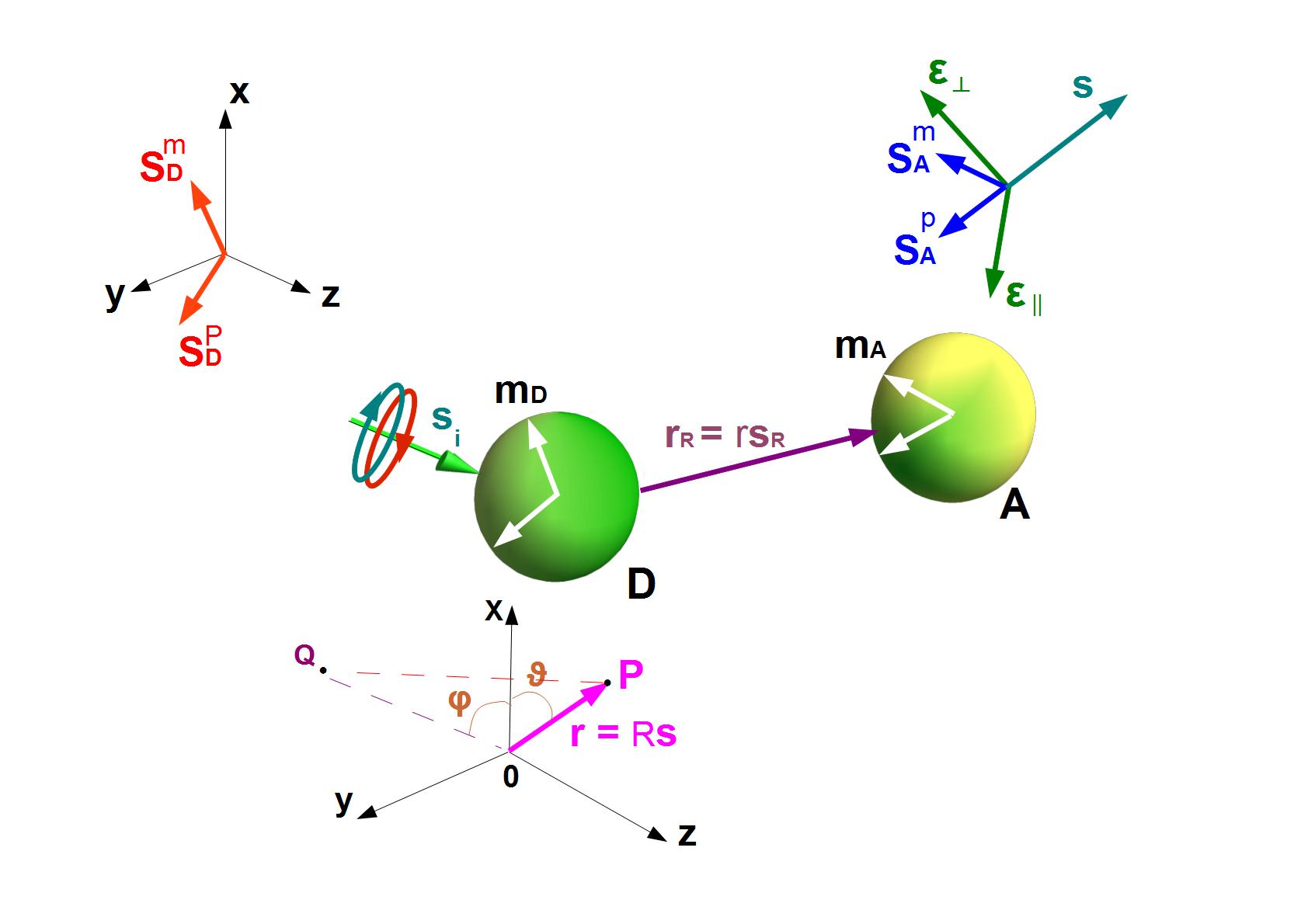
Figure 2: (Color online). In the $OXYZ$ framework an elliptically polarized plane wave, propagating along ${\bf s}_{i}=\hat{\bm{z}}$, incides on a donor particle D. The fields emitted by the dipoles moments, oriented along ${\bf s}_{D}^{p}$ and ${\bf s}_{D}^{m}$, are evaluated at a generic point $P$: ${\bf r}=R\bf s$ , $|{\bf s}|=1$, of coordinates $(R,\theta,\phi)$ which eventually coincides with the center of the acceptor A with dipoles moments oriented along ${\bf s}_{A}^{p}$ and ${\bf s}_{A}^{m}$, thus becoming ${\bf r}={\bf r}_{A}$. The point $Q$ is the projection of $P$ on the plane $OXY$; the scattering plane being $OPQ$. We show the three orthonormal vectors: ${\bf s}$, ${\bm{\epsilon}}_{\parallel}$ (in the plane $OPQ$ and in the sense of rotation of $\theta$), and ${\bm{\epsilon}}_{\perp}$ (normal to $OPQ$). which form the helicity basis for the fields ${\bf E}_{D}({\bf r}_{A}),\,\,{\bf B}_{D}({\bf r}_{A})$ in A: $\{\hat{\bm{\eta}}^{+},\hat{\bm{\eta}}^{-}\}$, $\hat{\bm{\eta}}^{\pm}=\frac{1}{\sqrt{2}}(\hat{\bf e}_{\perp}\pm i\hat{\bf e}_{\parallel})$; while that for the field incident on D is $\{\hat{\bm{\epsilon}}^{+},\hat{\bm{\epsilon}}^{-}\}$, ${\bm{\epsilon}}^{\pm}=(1/\sqrt{2})(\hat{\bf x}\pm i\hat{\bf y})$.

As for the acceptor dipole moments ${\bf p}_{A}=p_{A}{\bf s}_{A}^{p}$ and ${\bf m}_{A}=m_{A}{\bf s}_{A}^{m}$ , making the generic point $P$ to coincide with the center of the acceptor, i.e. ${\bf r}={\bf r}_{A}$, we consider the origin of coordinates $O$, and therefore the orientation of the unit vector ${\bf s}={\bf r}_{A}/r_{A}$, such that without loss of generality both ${\bf s}_{A}^{p}$ and ${\bf s}_{A}^{m}$ vary in the plane defined by the vectors $\hat{\bf e}_{\perp}$ and $\hat{\bf e}_{\parallel}$, normal to its position unit vector ${\bf s}=(\sin\theta\cos\phi,\sin\theta\sin\phi,\cos\theta)$, as shown in Fig. 2. Notice that the orientations of ${\bf s}$ and ${\bf s}_{R}$ are not linked to each other, which will later be important for calculating the orientational averages of the ${\cal K}$ - factors. Therefore we write, (cf. Fig. 2):

$${\bf p}_{A}=p_{A}{\bf s}_{A}^{p},\,p_{A}=|{\bf p}_{A}|,\,{\bf s}_{A}^{p}=s_{A\,\perp}^{p}\hat{\bf e}_{\perp}+s_{A\,\parallel}^{p}\hat{\bf e}_{\parallel};$$

$${\bf s}_{A}^{m}=s_{A\,\perp}^{m}\hat{\bf e}_{\perp}+s_{A\,\parallel}^{m}\hat{\bf e}_{\parallel}=\zeta_{\perp}s_{A\,\perp}^{p}\hat{\bf e}_{\perp}+\zeta_{\parallel}s_{A\,\parallel}^{p}\hat{\bf e}_{\parallel}.\,\,\,\,\,$$ (37)

$$|s_{A\,\perp}^{m}|^{2}+|s_{A\,\parallel}^{m}|^{2}=|\zeta_{\perp}|^{2}|s_{A\,\perp}^{p}|^{2}+|\zeta_{\parallel}|^{2}|s_{A\,\parallel}^{p}|^{2}=1.\,\,\,\,\,\,\,\,\,\,\,\,\,\,\,\,\,\,$$ (38)

And the unitarity of both ${\bf s}_{A}^{p}$ and ${\bf s}_{A}^{m}$ imply $|\zeta_{\perp}|=|\zeta_{\parallel}|=1$.

Since

$$\hat{\bf e}_{\perp}=\cos\theta\cos\phi\,\hat{\bf x}+\cos\theta\sin\phi\,\hat{\bf y}-\sin\theta\,\hat{\bf z},$$

$$\hat{\bf e}_{\parallel}=\sin\phi\,\hat{\bf x}-\cos\phi\,\hat{\bf y}.$$ (39)

${\bf s}_{A}^{p}$ referred to the $\hat{\bf x},\hat{\bf y},\hat{\bf z}$ basis is

$${\bf s}_{A}^{p}=({s}_{A\,\perp}^{p}\sin\phi+{s}_{A\,\parallel}^{p}\cos\theta\cos\phi)\hat{\bf x}$$

$$+(-{s}_{A\,\perp}^{p}\cos\phi+{s}_{A\,\parallel}^{p}\cos\theta\sin\phi)\hat{\bf y}-{s}_{A\,\parallel}^{p}\sin\theta\,\hat{\bf z}.\,\,\,$$ (40)

And from (37) we have for the acceptor magnetic dipole moment ${\bf m}_{A}=m_{A}{\bf s}_{A}^{m}$:

$${\bf s}_{A}^{m}=(\zeta_{\perp}{s}_{A\,\perp}^{p}\sin\phi+\zeta_{\parallel}{s}_{A\,\parallel}^{p}\cos\theta\cos\phi)\hat{\bf x}$$

$$-(\zeta_{\perp}{s}_{A\,\perp}^{p}\cos\phi-\zeta_{\parallel}{s}_{A\,\parallel}^{p}\cos\theta\sin\phi)\hat{\bf y}-\zeta_{\parallel}{s}_{A\,\parallel}^{p}\sin\theta\,\hat{\bf z}.\,\,\,\,\,,$$ (41)

The components ${s}_{A\,\perp}^{p}$ and ${s}_{A\,\parallel}^{p}$ of the unit vector ${\bf s}_{A}^{p}$ define the plane of reference of rotation of A which contain $\hat{\bf e}_{\perp}$ and $\hat{\bf e}_{\parallel}$, [cf. Eqs. (37)], yielding the helicity basis $\{\hat{\bm{\eta}}^{+},\hat{\bm{\eta}}^{-}\}$: $\hat{\bm{\eta}}^{\pm}=\frac{1}{\sqrt{2}}(\hat{\bf e}_{\perp}\pm i\hat{\bf e}_{\parallel})$, $({\bm{\eta}}^{\pm\,*}\cdot{\bm{\eta}}^{\mp}=0)$, (see Fig. 2). So that

$${\bf p}_{A}=p_{A}^{+}\hat{\bm{\eta}}^{+}+p_{A}^{-}\hat{\bm{\eta}}^{-}=p_{A}{\bf s}_{A}^{p}.$$

$${\bf m}_{A}=m_{A}^{+}\hat{\bm{\eta}}^{+}+m_{A}^{-}\hat{\bm{\eta}}^{-}=m_{A}{\bf s}_{A}^{m}.$$ (42)

And then

$$p_{A}=[|p_{A}^{+}|^{2}+|p_{A}^{-}|^{2}]^{\frac{1}{2}};\,\,\,\,{\bf s}_{A}^{p}=p_{A}^{-1}[p_{A}^{+}\hat{\bm{\eta}}^{+}+p_{A}^{-}\hat{\bm{\eta}}^{-}];$$

$$|{\bf s}_{A}^{p}|^{2}={s}_{A\,i}^{p}\,{s}_{A\,i}^{p\,*}=1.$$ (43)

$$m_{A}=[|m_{A}^{+}|^{2}+|m_{A}^{-}|^{2}]^{\frac{1}{2}};\,\,\,\,{\bf s}_{A}^{m}=m_{A}^{-1}[m_{A}^{+}\hat{\bm{\eta}}^{+}+m_{A}^{-}\hat{\bm{\eta}}^{-}];$$

$$|{\bf s}_{A}^{m}|^{2}={s}_{A\,i}^{m}\,s_{A\,i}^{m\,*}=1.\,\,\,\,\,$$ (44)

Again we see that, like for the donor, the amplitudes $p_{A}$ and $m_{A}$ of the acceptor dipole moments in this configuration are real rather than complex.

The $s_{A\,\perp}^{p}$ and $s_{A\,\parallel}^{p}$ components are according to (42)-(44):

$$s_{A\,\perp}^{p}=\frac{1}{p_{A}\sqrt{2}}(p_{A}^{+}+p_{A}^{-});\,\,\,\,s_{A\,\parallel}^{p}=\frac{i}{p_{A}\sqrt{2}}(p_{A}^{+}-p_{A}^{-}).$$ (45)

With analogous expressions for $s_{A\,\perp}^{m}$ and $s_{A\,\parallel}^{m}$ on substituting $p$ by $m$.

On the other hand, from (43)-(45):

$$|{s}_{A\,\perp,\,\parallel}^{p}|^{2}=\frac{1}{2}\pm\frac{\mbox{Re}\{p_{A}^{+}p_{A}^{-\,*}\}}{p_{A}^{2}};\,\,$$

$$|{s}_{A\,\perp,\,\parallel}^{m}|^{2}=\frac{1}{2}\pm\frac{\mbox{Re}\{m_{A}^{+}m_{A}^{-\,*}\}}{m_{A}^{2}}.\,\,\,\,$$ (46)

Where the upper and lower sign in $\pm$ apply to $\perp$ and $\parallel$, respectively.

V.3 Transfer of helicity and energy. Interaction radii

Finally, since according to (27) and (28) $p_{D}$ and $m_{D}$ are now real, and so are ${\cal K}^{(1)}$ and ${\cal K}^{(2)}$, the helicity and energy, transferred from D to A, [cf. Eqs.(15) and (16)] become

$${\cal W}_{\mathscr{H}}^{DA}=\frac{2\pi c}{\epsilon r^{6}}[p_{D}m_{D}\mbox{Re}\{-\frac{\alpha_{e}^{A}}{\epsilon}{\cal K}^{(1)}_{\cal H}\,\,\,\,\,\,$$

$$+\mu\alpha_{m}^{A}{\cal K}^{(2)}_{\cal H}\}+\mu m_{D}^{2}\mbox{Re}\{\alpha_{me}^{A}\,{\cal K}^{(3)}_{\cal H}\}+\frac{p_{D}^{2}}{\epsilon}\mbox{Re}\{\alpha_{me}^{A}\,{\cal K}^{(4)}_{\cal H}\}].\,\,\,\,\,\,$$ (47)

$${\cal W}^{DA}=\frac{\omega}{2r^{6}}[\frac{\mbox{Im}\{\alpha_{e}^{A}\}}{\epsilon^{2}}\,p_{D}^{2}\,{\cal K}^{(1)}+\mu^{2}\mbox{Im}\{\alpha_{m}^{A}\}\,m_{D}^{2}\,{\cal K}^{(2)}$$

$$-2\frac{\mu}{\epsilon}p_{D}m_{D}\mbox{Re}\{\alpha_{me}^{A}\}\mbox{Im}\{{\cal K}^{(3)}\}].\,\,\,\,\,\,\,\,\,\,\,\,\,\,\,\,\,\,$$ (48)

Once again, while Eq. (47) accounts for a transfer of helicity between D and A, either positive or negative as a consequence of the handedness of A and D, a negative transferred energy ${\cal W}^{DA}$ may exist, in contrast with conventional FRET, when the last term of (48) is larger than the sum of the first two terms.

The interaction radii $R_{\mathscr{H}}$ and $R_{\cal E}$ now read

$$R_{\mathscr{H}}^{6}=\frac{3}{4k^{3}}\,|p_{D}m_{D}\mbox{Re}\{-\frac{\alpha_{e}^{A}}{\epsilon}{\cal K}^{(1)}_{\cal H}+\mu\alpha_{m}^{A}{\cal K}^{(2)}_{\cal H}\}$$

$$+\mu m_{D}^{2}\mbox{Re}\{\alpha_{me}^{A}\,{\cal K}^{(3)}_{\cal H}\}+\frac{p_{D}^{2}}{\epsilon}\mbox{Re}\{\alpha_{me}^{A}\,{\cal K}^{(4)}_{\cal H}\}|$$

$$/|\mbox{Im}(p_{D}^{+}m_{D}^{+\,*}+p_{D}^{-}m_{D\,*}^{-})|\,\,\,\,\,.$$ (49)

$$R_{\cal E}^{6}=\frac{3}{2k^{3}}|\frac{\mbox{Im}\{\alpha_{e}^{A}\}}{\epsilon^{2}}\,p_{D}^{2}\,{\cal K}^{(1)}+\mu^{2}\mbox{Im}\{\alpha_{m}^{A}\}\,m_{D}^{2}\,{\cal K}^{(2)}$$

$$-2\frac{\mu}{\epsilon}p_{D}m_{D}\mbox{Re}\{\alpha_{me}^{A}\}\mbox{Im}\{{\cal K}^{(3)}\}|/(\frac{p_{D}^{2}}{\epsilon}+\mu m_{D}^{2}).\,\,\,\,\,\,\,$$ (50)

V.4 Orientational averages of the ${\cal K}$-factors

The orientation of the dipole moments of D and A often randomly vary, so that the relative axes of rotation between D and A is unknown. In this case it is pertinent to work with the orientational averages of the ${\cal K}$-factors.

Using the form of the several unit vectors ${\bf s}_{A}$ and ${\bf s}_{D}$ shown above, these averages are

$$<{\cal K}^{(1)}_{\cal H}>=\frac{1}{10}\{7|{s}_{A\,\perp}^{p}|^{2}+\frac{19}{3}|{s}_{A\,\parallel}^{p}|^{2}\}\{\xi_{x}^{*}|s_{D\,x}^{p}|^{2}$$

$$+\xi_{y}^{*}|s_{D\,y}^{p}|^{2}\}.\,\,\,\,\,$$ (51)

$$<{\cal K}^{(2)}_{\cal H}>=\{\frac{7}{10}(|\zeta_{\perp}|^{2}|{s}_{A\,\perp}^{p}|^{2}+\frac{1}{3}|\zeta_{\parallel}|^{2}|{s}_{A\,\parallel}^{p}|^{2})\,\,\,\,\,\,\,\,\,\,\,\,\,\,\,\,\,\,\,\,\,\,\,\,\,\,\,\,\,\,\,\,$$

$$+\frac{2}{5}|\zeta_{\parallel}|^{2}|{s}_{A\,\parallel}^{p}|^{2}\}\{\xi_{x}|s_{D\,x}^{p}|^{2}+\xi_{y}|s_{D\,y}^{p}|^{2}\}=\frac{1}{10}\{7|{s}_{A\,\perp}^{p}|^{2}\,\,$$

$$+\frac{19}{3}|{s}_{A\,\parallel}^{p}|^{2}\}\{\xi_{x}|s_{D\,x}^{p}|^{2}+\xi_{y}|s_{D\,y}^{p}|^{2}\}=<{\cal K}^{(1)\,*}_{\cal H}>.\,\,\,\,\,\,\,\,\,\,\,\,\,\,\,\,\,\,\,\,\,\,\,$$ (52)

$$<{\cal K}^{(3)}_{\cal H}>=\frac{1}{10}(7\zeta_{\perp}^{\,*}|{s}_{A\,\perp}^{p}|^{2}+\frac{19}{3}\zeta_{\parallel}^{\,*}|{s}_{A\,\parallel}^{p}|^{2}).\,\,$$ (53)

$$<{\cal K}^{(4)}_{\cal H}>=\frac{1}{10}(7\zeta_{\perp}|{s}_{A\,\perp}^{p}|^{2}+\frac{19}{3}\zeta_{\parallel}|{s}_{A\,\parallel}^{p}|^{2})=<{\cal K}^{(3)\,*}_{\cal H}>.\,\,\,\,$$ (54)

$$<{\cal K}^{(1)}>=\frac{1}{10}(7|{s}_{A\,\perp}^{p}|^{2}+\frac{19}{3}|{s}_{A\,\parallel}^{p}|^{2}).$$ (55)

$$<{\cal K}^{(2)}>=\frac{7}{10}(|\zeta_{\perp}|^{2}|{s}_{A\,\perp}^{p}|^{2}+\frac{1}{3}|\zeta_{\parallel}|^{2}|{s}_{A\,\parallel}^{p}|^{2})\,\,\,\,\,\,\,\,\,\,\,\,\,\,\,$$

$$+\frac{2}{5}|\zeta_{\parallel}|^{2}|{s}_{A\,\parallel}^{p}|^{2}=\frac{1}{10}(7|{s}_{A\,\perp}^{p}|^{2}+\frac{19}{3}|{s}_{A\,\parallel}^{p}|^{2})=<{\cal K}^{(1)}>.\,\,\,\,\,$$ (56)

$$<{\cal K}^{(3)}>=\frac{1}{10}\{7\zeta_{\perp}^{\,*}|{s}_{A\,\perp}^{p}|^{2}+\frac{19}{3}\zeta_{\parallel}^{\,*}|{s}_{A\,\parallel}^{p}|^{2}\}$$

$$\times\{\xi_{x}|s_{D\,x}^{p}|^{2}+\xi_{y}|s_{D\,y}^{p}|^{2}\}.\,\,\,\,\,\,\,\$$ (57)

The procedure to calculate thes orientational averages is illustrated in Appendix 4.

Notice that these averages have been written in terms of the components of ${\bf s}_{D}^{p}$ and ${\bf s}_{A}^{p}$, as well as of ${\bm{\xi}}$ and ${\bm{\zeta}}$. The latter characterizing the respective orientation of ${\bf s}_{D}^{m}$ and ${\bf s}_{A}^{m}$ relative to that of ${\bf s}_{D}^{p}$ and ${\bf s}_{A}^{p}$, as shown before.

We can further average the quantities $|s_{D\,x,\,y}^{p}|^{2}$ and $|{s}_{A\,\perp,\,\parallel}^{p}|^{2}$ in the respective plane of rotation of ${\bf s}_{D}^{p}$ and ${\bf s}_{A}^{p}$. According to Eqs. (30) and (37), on expressing the two components of these unit vectors in polar coordinates as a cosine and a sine of the rotation angle, these averages are: $<|s_{D\,x,\,y}^{p}|^{2}>=<|{s}_{A\,\perp,\,\parallel}^{p}|^{2}>=1/2$. Hence, with this additional averaging, the orientational mean ${\cal K}$-factors finally become

$$<{\cal K}^{(1)}_{\cal H}>=\frac{1}{3}(\xi_{x}^{*}+\xi_{y}^{*}),$$ (58)

$$<{\cal K}^{(2)}_{\cal H}>=\frac{1}{3}(\xi_{x}+\xi_{y})=<{\cal K}^{(1)\,*}_{\cal H}>.\,\,\,\,$$ (59)

$$<{\cal K}^{(3)}_{\cal H}>=\frac{1}{20}(7\zeta_{\perp}^{\,*}+\frac{19}{3}\zeta_{\parallel}^{\,*}).\,\,\,\,\,\,\,\,\,\,\,\,\,\,\,\,\,\,\,\,\,\,$$ (60)

$$<{\cal K}^{(4)}_{\cal H}>=\frac{1}{20}(7\zeta_{\perp}+\frac{19}{3}\zeta_{\parallel})=<{\cal K}^{(3)\,*}_{\cal H}>.\,\,\,\,\,\,\,\,\,\,\,\,\,\$$ (61)

$$<{\cal K}^{(1)}>=\frac{2}{3}=<{\cal K}^{(2)}>,\,\,\,\,\,\,\,\,\,\,\,\,\,$$

$$<{\cal K}^{(3)}>=\frac{1}{40}(7\zeta_{\perp}^{\,*}+\frac{19}{3}\zeta_{\parallel}^{\,*})(\xi_{x}+\xi_{y}).\,\,\,\,\,\,\,\$$ (62)

Therefore these averages are expressed in terms of the relative orientations of the magnetic moments with respect to the electric ones, both in D and A. For example, in the particular case in which $\xi_{x}=\xi_{y}=1$, $\zeta_{\perp}=\zeta_{\parallel}=1$, (i.e. both D and A being linearly polarized right dipoles), each of these quantities would reduce to $2/3$. On the other hand, when ${\bf m}_{D}={\bf m}_{A}=0$, the only polarizability of the acceptor different from zero is $\alpha_{e}^{A}$; hece Eq. (47) yields no transfer of helicity: ${\cal W}_{\mathscr{H}}^{DA}=0$, while Eq. (48) reproduces the energy transfer $W^{DA}$ of standard FRET with $<{\cal K}^{(1)}>=2/3=\kappa^{2}$.

V.5 Case in which donor and acceptor have well defined helicity

We now address the RHELT and RET, Eqs. (47) and (48), with deterministically oriented dipole moments of D and A. Let us assume well defined helicity (WDH) nieto3 ; corbato1 ; gutsche4 in the illumination of D, for example let a CPL plane wave be incident on the donor. Then in (27) and (28) either $p_{D}^{+}=0$ or $p_{D}^{-}=0$ depending on whether this illumination is RCP or LCP, respectively. Therefore the induced electric and magnetic dipole moments of D rotate in the $OXY$-plane, (cf. Fig. 2). The near field along the $OZ$ axis emitted by D is circularly polarized nieto3 : ${\bf E}_{nf}(\hat{\bm{z}})=-(k^{2}/\epsilon r^{3})p^{\pm}\hat{\bm{\epsilon}}^{\pm}$,    ${\bf B}_{nf}(\hat{\bm{z}})=\mp in{\bf E}_{nf}(\hat{\bm{z}})$.

As an instance. we consider in the $OXYZ$ framework: ${\bf s}_{R}=(0,0,1)$, (see Fig. 2), the field incident on D being CPL. The dipoles ${\bf p}_{D}$ and ${\bf m}_{D}$ rotate in the plane OXY, while ${\bf p}_{A}$ and ${\bf m}_{A}$ do it in a plane parallel to OXY at distance $|{\bf r}_{R}|=z=r$, ($|{\bf s}_{R}|=1$). I.e. From (32) we have: ${\bf s}_{D}^{p}=\exp(i\phi_{e}^{\pm}){\bm{\epsilon}}^{\pm}=\frac{\exp(i\phi_{e}^{\pm})}{\sqrt{2}}(1,\pm i,0)$, ${\bf s}_{D}^{m}=\exp[i(\phi_{m}^{\pm}-\phi_{e}^{\pm})]{\bf s}_{D}^{p}$.

On the other hand, from (37), (42), (43) and (44) we have for the acceptor

$${\bf p}_{A}^{\pm}=p_{A}^{\pm}\hat{\bm{\eta}}^{\pm},\,{\bf m}_{A}^{\pm}=m_{A}^{\pm}\hat{\bm{\eta}}^{\pm};\,{\bf s}_{A}^{p}=e^{i\psi_{e}^{\pm}}\hat{\bm{\eta}}^{\pm},\,{\bf s}_{A}^{m}=e^{i\psi_{m}^{\pm}}\hat{\bm{\eta}}^{\pm}.\,\,\,$$ (63)

$\psi_{e}^{\pm}$ and $\psi_{m}^{\pm}$ representing the arguments of the complex scalars $p_{A}^{\pm}$ and $m_{A}^{\pm}$, respectively. Hence

$${\bf s}_{A}^{m}=e^{i(\psi_{m}^{\pm}-\psi_{e}^{\pm})}{\bf s}_{A}^{p}.$$ (64)

Therefore the following values hold:

$${s}_{A\,\perp}^{p,m}=\frac{e^{i\psi_{e,m}^{\pm}}}{\sqrt{2}},\,\,\,\,{s}_{A\,\parallel}^{p,m}=\pm i\frac{e^{i\psi_{e,m}^{\pm}}}{\sqrt{2}},\,\,\,\,$$

$$|{s}_{A\,\perp}^{p}|^{2}=|{s}_{A\,\parallel}^{p}|^{2}=|{s}_{A\,\perp}^{m}|^{2}=|{s}_{A\,\parallel}^{m}|^{2}=\frac{1}{2}.$$ (65)

Let ${\bf s}_{A}^{p}$ be rotated with respect to ${\bf s}_{D}^{p}$ in the $XY$-plane by an angle $\Theta$; namely, ${\bf s}_{A}^{p}=\exp(i\alpha){\bf R}{\bf s}_{D}^{p}$. $\alpha$ being a phase shift and ${\bf R}$ denoting the rotation matrix:

$${\bf R}=\left[{\begin{array}[]{cc}\cos\Theta&-\sin\Theta\\ \sin\Theta&\cos\Theta\\ \end{array}}\right].$$ (68)

According to (31) and (63), both ${\bf s}_{D}^{p}$ and ${\bf s}_{A}^{p}$ are helicity vectors aside from a phase factor, hence ${\bf R}{\bf s}_{D}^{p}=\exp(\mp i\Theta){\bf s}_{D}^{p}$, and $|{\bf s}_{A}^{p}\cdot{\bf s}_{D}^{p}|^{2}=0$.

Then for these magnetoelectric dipoles one has from (8) - (14):

$${\cal K}^{(1)}={\cal K}^{(2)}=|{\bf s}_{D}^{p}\cdot{\bf s}_{A}^{p}|^{2},\,\,\,\,\,\,\,\,$$

$${\cal K}^{(3)}=|{\bf s}_{D}^{p}\cdot{\bf s}_{A}^{p}|^{2}\exp\{i[(\phi_{m}^{\pm}-\phi_{e}^{\pm})-(\psi_{m}^{\pm}-\psi_{e}^{\pm})]\},\,\,\,\,$$

$${\cal K}_{\cal H}^{(1)}=|{\bf s}_{A}^{p}\cdot{\bf s}_{D}^{p\,*}|^{2}\exp[-i(\phi_{m}^{\pm}-\phi_{e}^{\pm})],\,\,\,\,\,\,\,\,\,\,\,\,\,\,\,\,$$

$${\cal K}_{\cal H}^{(2)}=|{\bf s}_{D}^{p}\cdot{\bf s}_{A}^{p}|^{2}\exp[i(\phi_{m}^{\pm}-\phi_{e}^{\pm})],\,\,\,\,\,\,\,\,\,$$

$${\cal K}_{\cal H}^{(3)}=|{\bf s}_{D}^{p}\cdot{\bf s}_{A}^{p}|^{2}\exp[-i(\psi_{m}^{\pm}-\psi_{e}^{\pm})],\,\,\,\,\,\,\,\,$$

$${\cal K}_{\cal H}^{(4)}=|{\bf s}_{D}^{p}\cdot{\bf s}_{A}^{p}|^{2}\exp[i(\psi_{m}^{\pm}-\psi_{e}^{\pm})].\,\,\,\,$$ (69)

But $|{\bf s}_{D}^{p}\cdot{\bf s}_{A}^{p}|^{2}=1$, hence (47) and (48) become

$${\cal W}_{\mathscr{H}}^{DA}=\frac{2\pi c}{\epsilon r^{6}}[p_{D}m_{D}\mbox{Re}\{-\frac{\alpha_{e}^{A}}{\epsilon}e^{-i(\phi_{m}^{\pm}-\phi_{e}^{\pm})}+\mu\alpha_{m}^{A}e^{i(\phi_{m}^{\pm}-\phi_{e}^{\pm})}\}$$

$$+\mu m_{D}^{2}\mbox{Re}\{\alpha_{me}^{A}\,e^{-i(\psi_{m}^{\pm}-\psi_{e}^{\pm})}\}+\frac{p_{D}^{2}}{\epsilon}\mbox{Re}\{\alpha_{me}^{A}\,e^{i(\psi_{m}^{\pm}-\psi_{e}^{\pm})}\}].\,\,\,\,\,\,$$ (70)

$${\cal W}^{DA}=\frac{\omega}{2r^{6}}[\frac{\mbox{Im}\{\alpha_{e}^{A}\}}{\epsilon^{2}}\,p_{D}^{2}\,+\mu^{2}\mbox{Im}\{\alpha_{m}^{A}\}\,m_{D}^{2}\,\,\,\,\,\,\,$$

$$-2\frac{\mu}{\epsilon}p_{D}m_{D}\mbox{Re}\{\alpha_{me}^{A}\}\sin[(\phi_{m}^{\pm}-\phi_{e}^{\pm})-(\psi_{m}^{\pm}-\psi_{e}^{\pm})].\,\,\,\,\,\,$$ (71)

And again ${\cal W}^{DA}$ may become negative for large enough $\Re\{\alpha_{me}^{A}\}$, and oscillate with the difference of phase-shifts of ${\bf s}_{D}^{m}$ and ${\bf s}_{D}^{p}$, and of ${\bf s}_{A}^{m}$ and ${\bf s}_{A}^{p}$. The radii $R_{\mathscr{H}}$ and $R_{\cal E}$ are now given by:

$$R_{\mathscr{H}}^{6}=\frac{3}{4k^{3}}\,|p_{D}m_{D}\mbox{Re}\{-\frac{\alpha_{e}^{A}}{\epsilon}e^{-i(\phi_{m}^{\pm}-\phi_{e}^{\pm})}\,\,\,\,\,\,\,\,\,\,\,\,\,\,\,\,\,\,\,\,\,\,\,\,\,\,\,\,\,\,\,\,\,$$

$$+\mu\alpha_{m}^{A}e^{i(\phi_{m}^{\pm}-\phi_{e}^{\pm})}\}+\mu m_{D}^{2}\mbox{Re}\{\alpha_{me}^{A}\,e^{-i(\psi_{m}^{\pm}-\psi_{e}^{\pm})}\}\,\,\,\,\,\,\,\,\,\,\,\,\,\,\,\,\,\,\,\,$$

$$+\frac{p_{D}^{2}}{\epsilon}\mbox{Re}\{\alpha_{me}^{A}e^{i(\psi_{m}^{\pm}-\psi_{e}^{\pm})}\}|/p_{D}m_{D}|\sin(\phi_{e}^{\pm}-\phi_{m}^{\pm})|.\,\,\,\,\,\,\,\,\,\,$$ (72)

$$R_{\cal E}^{6}=\frac{3}{2k^{3}}\,\,|\frac{\mbox{Im}\{\alpha_{e}^{A}\}}{\epsilon^{2}}\,p_{D}^{2}\,+\mu^{2}\mbox{Im}\{\alpha_{m}^{A}\}\,m_{D}^{2}\,\,\,\,\,\,\,$$

$$-2\frac{\mu}{\epsilon}p_{D}m_{D}\,\mbox{Re}\{\alpha_{me}^{A}\}\sin[(\phi_{m}^{\pm}-\phi_{e}^{\pm})-(\psi_{m}^{\pm}-\psi_{e}^{\pm})]|$$

$$/(\frac{p_{D}^{2}}{\epsilon}+\mu m_{D}^{2}).\,\,\,\,\,\,\,\,\,\,\,\,\,\,\,\,\,\,\,\,\,\,\,\,\,\,\,\,\,\,$$ (73)

Notice that while in conventional FRET if D and A have dipoles linearly polarized in planes normal to ${\bf s}_{R}$, there is no energy transfer if ${\bf s}_{D}^{p}$ and ${\bf s}_{A}^{p}$ are perpendicular to each other, i.e. ${\cal K}^{(1)}=0$, this is not the case in the configuration of circularly rotating dipoles in D and A, since, as seen above, in this latter case the unit vectors ${\bf s}_{A}^{p}$ and ${\bf s}_{D}^{p}$ are complex and $|{\bf s}_{A}^{p}\cdot{\bf s}_{D}^{p}|^{2}=1$.

V.6 Consequences when D and/or A is dual

V.6.1 1. a. The dipoles induced in both and A are dual

In this case ${\epsilon}^{-1}\alpha_{e}^{A}=\mu\alpha_{m}^{A}$; ${\epsilon}^{-1}\alpha_{e}^{D}=\mu\alpha_{m}^{D}$. From (27), (28), (42), (43) and (44) one has $p_{D}^{\pm}=\pm inm_{D}^{\pm}$, and $p_{A}^{\pm}=\pm inm_{A}^{\pm}$, and both D and A emit fields of well defined helicity nieto3 ; corbato1 ; gutsche4 , (e.g. CPL fields for incident CPL illumination). Then ${\bf s}_{D}^{m}=\mp i{\bf s}_{D}^{p}$, and ${\bf s}_{A}^{m}=\mp i{\bf s}_{A}^{p}$. I.e. $\phi_{m}^{\pm}-\phi_{e}^{\pm}$ and $\psi_{m}^{\pm}-\psi_{e}^{\pm}$ are either $3\pi/2$ for the upper (+) sign and $\pi/2$ for the lower (-) sign. Hence one has that $(\phi_{m}^{\pm}-\phi_{e}^{\pm})-(\psi_{m}^{\pm}-\psi_{e}^{\pm})$ is either $0$ or $\pi$. Also $p_{D}=nm_{D}$.

Then ${\cal W}^{DA}$, given by (71) becomes

$${\cal W}^{DA}=\frac{\omega}{\epsilon^{2}r^{6}}p_{D}^{2}\mbox{Im}\{\alpha_{e}^{A}\}.$$ (74)

Also, the sum of the third and fourth terms of (70) also vanishes since $\cos(\psi_{m}^{\pm}-\psi_{e}^{\pm})=0$, and therefore

$${\cal W}_{\mathscr{H}}^{DA}=\pm\frac{4\pi c}{\epsilon^{2}r^{6}}\,p_{D}^{2}\,\frac{\mbox{Im}\{\alpha_{e}^{A}\}}{n}.\,\,\,\,\,\,\,\,\,\,\,\,$$ (75)

Therefore the RET and RHELT rates are equivalent apart from a constant, and are functionally similar to the transfer of energy of a standard FRET with circularly polarized D and A when one considers in (75) the effective polarizability given by Eq. (22). This result is consistent with the fact that in this case the light emitted by both D and A is circularly polarized and, therefore, there is an equivalence, apart from a constant factor, between the extinction of helicity and of energy cameron1 ; nieto2 ; nieto3 .

This is manifested by the radii:

$$R_{\mathscr{H}}^{6}=\frac{3}{2\epsilon k^{3}}\mbox{Im}\{\alpha_{e}^{A}\},\,\,\,\,\,\,\,\,\,\,\,\,\,\,\,\,\,\,\,\,\,\,R_{\cal E}^{6}=\frac{3}{\epsilon k^{3}}\mbox{Im}\{\alpha_{e}^{A}\}.\,\,\,\,\,\,\,\,\,\,\,\,\,\,\,\,\,\,\,\,\,\,\,\,$$ (76)

Which makes $R_{\mathscr{H}}$ and $R_{\cal E}$ proportional to the radius of the acceptor, and $R_{\cal E}=1.12R_{\mathscr{H}}$.

V.6.2 1. b. Only A is dual

In this case (70) and (71) lead to

$${\cal W}_{\mathscr{H}}^{DA}=-\frac{4\pi c}{\epsilon^{2}r^{6}}p_{D}m_{D}\mbox{Im}\{\alpha_{e}^{A}\}\sin(\phi_{m}^{\pm}-\phi_{e}^{\pm}).$$ (77)

$${\cal W}^{DA}=\frac{ck}{2\epsilon nr^{6}}\{(\frac{p_{D}^{2}}{\epsilon}+\mu m_{D}^{2})\mbox{Im}\{\alpha_{e}^{A}\}\,\,\,\,\,\,\,$$

$$\mp 2\mu p_{D}m_{D}\mbox{Re}\{\alpha_{me}^{A}\}\cos(\phi_{m}^{\pm}-\phi_{e}^{\pm})\}.\,\,\,\,\,\,\,\,\,\,\,\,\,\,$$ (78)

Since now ${\cal W}_{\mathscr{H}}^{0}=8\pi ck^{3}p_{D}^{2}\sin(\phi_{m}^{\pm}-\phi_{e}^{\pm})/3\epsilon n$ and ${\cal W}^{0}=2ck^{4}p_{D}^{2}$, Eqs.(72) and (73) yield for the interaction radii:

$$R_{\mathscr{H}}^{6}=\frac{3}{2k^{3}\epsilon}\mbox{Im}\{\alpha_{e}^{A}\},$$ (79)

$$R_{\cal E}^{6}=\frac{3}{2\epsilon k^{3}}\{\mbox{Im}\{\alpha_{e}^{A}\}\,\,\,\,\,\,\,$$

$$\mp\frac{2\mu p_{D}m_{D}}{\frac{p_{D}^{2}}{\epsilon}+\mu m_{D}^{2}}|\mbox{Re}\{\alpha_{me}^{A}\}\cos(\phi_{m}^{\pm}-\phi_{e}^{\pm})|\}.\,\,\,\,$$ (80)

We see comparing (79) and (76) that when A is dual, $R_{\mathscr{H}}$ is not affected by whether D is dual or not. On the other hand, (80) is consistent with (76) since if D is also dual, $\cos(\phi_{m}^{\pm}-\phi_{e}^{\pm})=0$.

V.6.3 1.c. Only D is dual

Assuming for simplicity that $\epsilon=\mu=n=1$, we have from (47) and (71):

$${\cal W}_{\mathscr{H}}^{DA}=\frac{2\pi c}{r^{6}}p_{D}^{2}[\mp(\mbox{Im}\{\alpha_{e}^{A}\}+\mbox{Im}\{\alpha_{m}^{A}\})$$

$$+2\mbox{Re}\{\alpha_{me}^{A}\}\cos(\psi_{m}^{\pm}-\psi_{e}^{\pm})],$$ (81)

$${\cal W}^{DA}=\frac{ck}{2r^{6}}p_{D}^{2}\{\mbox{Im}\{\alpha_{e}^{A}\}+\mbox{Im}\{\alpha_{m}^{A}\}$$

$$\pm\mbox{Re}\{\alpha_{me}^{A}\}\cos(\psi_{m}^{\pm}-\psi_{e}^{\pm})\}.\,\,\,\,$$ (82)

Figure 3: (Color online). Both D and A are chiral and magnetoelectric. ${\bf p}_{D}$ and ${\bf m}_{D}$, are excited by elliptically polarized light. ${\bf p}_{A}$ and ${\bf m}_{A}$ are also elliptically polarized, (see text). $g=\frac{3r^{6}}{4a^{6}k^{3}(\lambda)}$. (a) $g{\cal W}_{\mathscr{H}}^{DA}(\lambda)$, ($k(\lambda)=n(\lambda)\frac{2\pi}{\lambda}$, $n(\lambda)=1$), and $g{\cal W}^{DA}(\lambda)$, with $a=15nm$ being the radius of D and A, and ${\cal W}_{\mathscr{H}}^{DA}$ and ${\cal W}^{DA}$ given by (47) and (48), respectively. Also shown are ${\cal P}_{\mathscr{H}}^{0}(\lambda)=\mbox{Im}[p_{D}^{+}m_{D}^{+\,*}+p_{D}^{-}m_{D}^{-\,*}]/a^{6}$ and ${\cal P}^{0}(\lambda)=(\frac{p_{D}^{2}}{\epsilon}+\mu m_{D}^{2})/a^{6}$, as well as $g{\cal W}_{\mathscr{H}}^{DA}/{\cal P}_{\mathscr{H}}^{0}$ and $g{\cal W}^{DA}/{\cal P}^{0}$. These quantities are plotted in arbitrary units. (b) $R_{\mathscr{H}}(\lambda)$ and $R_{\cal E}(\lambda)$ in $nm$. (c) and (d) Same as (a) and (b), respectively, with ${\bf p}_{A}$ and ${\bf m}_{A}$ randomly oriented with respect to ${\bf p}_{D}$ and ${\bf m}_{D}$, and the ${\cal K}$-factors being orientationally averaged.

And

$$R_{\mathscr{H}}^{6}=\frac{3}{4k^{3}}|\pm(\mbox{Im}\{\alpha_{e}^{A}\}+\mbox{Im}\{\alpha_{m}^{A}\})$$

$$+2\mbox{Re}\{\alpha_{me}^{A}\}\cos(\psi_{m}^{\pm}-\psi_{e}^{\pm})|,\,\,\,\,$$ (83)

$$R_{\cal E}^{6}=\frac{3}{2k^{3}}|\mbox{Im}\{\alpha_{e}^{A}\}+\mbox{Im}\{\alpha_{m}^{A}\}\pm\mbox{Re}\{\alpha_{me}^{A}\}\cos(\psi_{m}^{\pm}-\psi_{e}^{\pm})|,\,\,\,$$ (84)

which show the cosinusoidal oscillation of these RHELT and RET quantities with amplitude $\mbox{Re}\{\alpha_{me}^{A}\}$ about the level: $\pm(\mbox{Im}\{\alpha_{e}^{A}\}+\mbox{Im}\{\alpha_{m}^{A}\})$.

VI Examples: RHELT and RET when both donor and acceptor are chiral and magnetoelectric

VI.1 Example A: Donor is illuminated by an elliptically polarizated wavefield. The electric and magnetic dipole moments of the acceptor are elliptically polarized

We use Eqs. (47)-(50) on addressing chiral magnetoelectric D and A. Let the magnetic and cross electric-magnetic polarizabilities dominate in A. We assume the radius of both particles to be: $a\simeq 15nm$

Eqs. (A3-1) and (A3-2) of Appendix 3, with the parameters of Appendix 5, fit a model of donor emission spectra and acceptor extinction cross-sections. They are plotted in Fig.A5-1 (a) of Appendix 5. With these emission spectra, from Eqs.(A2-6)-(A2-13) of Appendix 2 one gets the donor and acceptor polarizabilities, shown in Figs.A5-1 (b) and (c) of Appendix 5.

We consider an elliptically polarized plane wave, propagating along $OZ$, incident on D, [cf. Fig. 2 and Eqs. (25)], with $e_{i}^{+}=7$ and $e_{i}^{-}=3$ [in arbitrary units (a.u.)]. The surrounding medium has $n(\lambda)=1$. Fig. A5-1(d) of Appendix 5 shows $p_{D}^{2}(\lambda)$, $m_{D}^{2}(\lambda)$ and $p_{D}(\lambda)m_{D}(\lambda)$, obtained from Eqs. (27) and (28) for this polarization. These latter equations show the transfer of incident angular momentum to the donor dipoles, and yield ${\bf p}_{D}$ and ${\bf m}_{D}$, as well as their respective unit vectors ${\bf s}_{D}^{p}$ and ${\bf s}_{D}^{m}$.

Figure 4: (Color online). Effect of the chirality of a magnetoelectric acceptor with elliptically polarized dipoles. Elliptic incident polarization. Same configuration as for Figs. 3 (a) and 3 (b). (a) $g{\cal W}_{\mathscr{H}}^{DA}(\lambda,\kappa)$ in arbitrary units. (b) $g{W}^{DA}(\lambda,\kappa)$ in arbitrary units. ($g=\frac{3r^{6}}{4a^{6}k^{3}(\lambda)})$. (c) $R_{\mathscr{H}}(\lambda,\kappa)$ in $nm$. (d) $R_{\cal E}(\lambda,\kappa)$ in $nm$. For $\kappa\in(0,-1]$, (not shown), the negative minima of $g{\cal W}_{\mathscr{H}}^{DA}/{\cal P}_{\mathscr{H}}^{0}$ and $g{\cal W}^{DA}/{\cal P}^{0}$ become positive maxima.

Figure 5: (Color online). The donor and the acceptor are chiral and magnetoelectric . Both ${\bf p}_{D}$ and ${\bf m}_{D}$, as well as ${\bf p}_{A}$ and ${\bf m}_{A}$, have well-defined helicity, (see text). (a) D and A have LCP dipole moments. $g{\cal W}_{\mathscr{H}}^{DA}(\lambda)$, and $g{\cal W}^{DA}(\lambda)$, ($k(\lambda)=n(\lambda)\frac{2\pi}{\lambda}$, $n(\lambda)=1$, $g=\frac{3r^{6}}{4a^{6}k^{3}(\lambda)}$), with $a=15nm$ being the radius of D and A, and ${\cal W}_{\mathscr{H}}^{DA}$ and ${\cal W}^{DA}$ given by (47) and (48), respectively. Also shown are ${\cal P}_{\mathscr{H}}^{0}(\lambda)=\mbox{Im}[p_{D}^{+}m_{D}^{+\,*}+p_{D}^{-}m_{D}^{-\,*}]/a^{6}$ and ${\cal P}^{0}(\lambda)=(\frac{p_{D}^{2}}{\epsilon}+\mu m_{D}^{2})/a^{6}$, as well as $g{\cal W}_{\mathscr{H}}^{DA}/{\cal P}_{\mathscr{H}}^{0}$ and $g{\cal W}^{DA}/{\cal P}^{0}$. (b) D and A with LCP moments. All these quantities are plotted in arbitrary units. $R_{\mathscr{H}}(\lambda)$ and $R_{\cal E}(\lambda)$ in $nm$. (c) and (d) Same as (a) and (b), respectively, when both D and A have RCP dipole moments.

The acceptor dipole moments ${\bf p}_{A}$ and ${\bf m}_{A}$, and their respective unit vectors ${\bf s}_{A}^{p}$ and ${\bf s}_{A}^{m}$, according to Eqs. (37) - (46) are set as $p_{A}^{\pm}=(\alpha_{e}^{A}\pm ni\alpha_{me}^{A})e^{\pm}$ and $m_{A}^{\pm}=(\alpha_{me}^{A}\mp ni\alpha_{m}^{A})e^{\pm}$, choosing $e^{+}=5a.u.$ and $e^{-}=-2a.u.$.

The overlapping integrals (22)-(24) for the effective polarizabilities: $\mbox{Im}\{\alpha_{e}^{A\,eff}\}$, $\mbox{Im}\{\alpha_{m}^{A\,eff}\}$ and $\mbox{Re}\{\alpha_{me}^{A\,eff}\}$, used in Eqs. (49) and (50) instead of their spectra: $\mbox{I}m\{\alpha_{e}^{A}(\lambda)\}$, $\mbox{Im}\{\alpha_{m}^{A}(\lambda)\}$ and $\mbox{R}e\{\alpha_{me}^{A}(\lambda)\}$, would yield a number for the RHELT and RET interaction radii. However, as mentioned before, we shall rather employ the polarizability spectra, whose variation with $\lambda$ gives us more information on the range of values of $R_{\mathscr{H}}(\lambda)$ and $R_{\cal E}(\lambda)$ on comparison with the spectra of D and A. In fact, the values of the polarizabilitiy spectra of A are in the same range as their effective values. This is seen on comparing Fig. A5-1(c) of Appendix 5 with these overlapping integrals (22)-(24) that yield: $\mbox{Im}\{\alpha_{e}^{A\,eff}\}=3.68\times 10^{3}$ $nm^{3}$, $\mbox{Im}\{\alpha_{m}^{A\,eff}\}=7.25\times 10^{3}$ $nm^{3}$, $\mbox{Re}\{\alpha_{me}^{A\,eff}\}=2.13\times 10^{4}$ $nm^{3}$.

Choosing ${\bf s}_{R}=(0,0,1)$, so that the basis $\{\hat{\bf e}_{\perp},\hat{\bf e}_{\parallel},{\bf s}\}$ becomes $\{\hat{\bf x},\hat{\bf y},\hat{\bf z}\}$, (cf. Fig. 2), we show in Fig. 3(a) the spectra ${\cal P}_{\mathscr{H}}^{0}(\lambda)=\mbox{Im}[p_{D}^{+}m_{D}^{+\,*}+p_{D}^{-}m_{D}^{-\,*}]/a^{6}$ and ${\cal P}^{0}(\lambda)=(\frac{p_{D}^{2}}{\epsilon}+\mu m_{D}^{2})/a^{6}$, as well as $g{\cal W}_{\mathscr{H}}^{DA}(\lambda)$ and $g{\cal W}^{DA}(\lambda)$; with ${\cal W}_{\mathscr{H}}^{DA}$ and ${\cal W}^{DA}$ given by (47) and (48), respectively, ($g=\frac{3r^{6}}{4a^{6}k^{3}(\lambda)}$, $k(\lambda)=n(\lambda)\frac{2\pi}{\lambda}$). All these functions have peaks at wavelengths near the the donor and acceptor dipole resonances, as seen on comparing Fig. 4(a) with the lineshapes of Figs. Figs. A5-1 (a) - (d) of Appendix 5. On the other hand, $g{\cal W}_{\mathscr{H}}^{DA}/{\cal P}_{\mathscr{H}}^{0}$ and $g{W}^{DA}/{\cal P}^{0}$, also shown in Fig. 3 (a), are less influenced by the maxima of the polarizability peaks of both D and A. This indicates that these latter quotients wash out to some extent the effect of these D and A resonant values. However $g{\cal W}_{\mathscr{H}}^{DA}/{\cal P}_{\mathscr{H}}^{0}$ has sharp spikes at wavelengths where ${\cal P}_{\mathscr{H}}^{0}(\lambda)=0$ by changing sign, a feature not always shared by $g{W}^{DA}/{\cal P}^{0}$ since ${\cal P}^{0}(\lambda)$ cannot be negative and rarely has zeros within its support.

It is remarkable that, as mentioned before, [cf. Eq.(48)], and due to the strong chirality of A, manifested by its large cross electric-magnetic polarizability $\alpha_{me}^{A}$, the transferred energy acquires negative values between $560$ and $630$ $nm$, [See.Fig. 3(a)], thus manifesting an increase, rather than a reduction, of the energy emitted by the donor in presence of the acceptor, (see next Section on Observables), a phenomenon ruled out in standard FRET and in RET between achiral particles.

Figures 3 (b) shows the radii $R_{\mathscr{H}}(\lambda)$ and $R_{\cal E}(\lambda)$. The former has larger values than the latter, and both are in ranges above $25$ $nm$ in the wavelength region between $490$ and $580$ $nm$. The large spikes in $R_{\mathscr{H}}(\lambda)$ coincide with those of $g{\cal W}_{\mathscr{H}}^{DA}/{\cal P}_{\mathscr{H}}^{0}(\lambda)$ again where ${\cal P}_{\mathscr{H}}^{0}(\lambda)=0$.

Finally, Figs. 3 (c) and 3 (d) show the same as Figs. 3 (a) and 3(b), respectively, when ${\bf p}_{A}$ and ${\bf m}_{A}$ are randomly oriented with respect to ${\bf p}_{D}$ and ${\bf m}_{D}$, and so is ${\bf s}_{R}$. In this case we have taken the orientational averages of all ${\cal K}$-factors according to Eqs. (58) - (62). The ${\cal K}$-averaging has a noticeable effect on both $R_{\cal E}(\lambda)$ and $R_{\mathscr{H}}(\lambda)$. As seen in the figures, the change is larger for the RHELT interaction radii.

If we adopted the criterion employed in connection to the case dealt with in Fig. A3-1 (b) of Appendix 3, namely choosig the wavelength at which the D and A lineshapes cross each other in Fig. A5-1 (a) of Appendix 5, we would get about $540nm$ for this wavelength and an estimation: $R_{\mathscr{H}}\simeq 48nm$ and $R_{\cal E}\simeq 44nm$ for the case studied in Fig. 3 (b), while $R_{\mathscr{H}}\simeq R_{\cal E}\simeq 30nm$ for the system addressed in Fig. 3 (d). As seen in Figs. 3(b) and 3(d), one can choose configurations in which at certain $\lambda$’s: $R_{\mathscr{H}}>>R_{\cal E}$; however, (and although not shown here for brevity), we have observed $R_{\mathscr{H}}<R_{\cal E}$ in some cases with either ${\bf s}_{R}=(1,0,0)$ or ${\bf s}_{R}=(1/\sqrt{2})(1,1,0)$. Also, on comparing with the standard FRET interaction radius: $5$ - $7.6$ $nm$ of the interacting molecules dealt with in Figs. A3-1 of Appendix 3, we see in Figs. 3 (b) and 3 (d) that larger particles convey greater RHELT and RET interaction radii, as we have observed in all our studied cases.

VI.1.1 Influence of the chirality of A

We choose the following variation of the real part of $\alpha_{me}^{A}(\omega)$, (cf. Eqs. (A2-7) of Appendix 2):

$$\alpha_{me}^{A\,R}(\omega)=\frac{2\pi}{k}\sqrt{\frac{\epsilon}{\mu}}\sigma_{me}^{A}(\omega)=\frac{\lambda}{n}\sqrt{\frac{\epsilon}{\mu}}\sigma_{me}^{A}(\omega).\,\,\,\omega=\frac{2\pi c}{\lambda}.\,\,\,\,\,$$ (85)

Where $\sigma_{me}^{A}(\omega)=\kappa\sigma_{me\,A}^{CD}(\omega).$

The $\kappa$-factor varies between $-1$ and $1$. In this regard, the polarizability $\alpha_{me}^{A\,R}(\omega)$ employed in Figs. 3 and in Figs. 5 (below) corresponds to $\kappa=3\cdot 50/2(4\pi)^{2}=0.47$.

The surfaces of Fig. 4 show the variation with $\lambda$ and $\kappa$ of $g{\cal W}_{\mathscr{H}}^{DA}(\lambda,\kappa)$, and $g{\cal W}^{DA}(\lambda,\kappa)$, as well as $R_{\mathscr{H}}(\lambda,\kappa)$ and $R_{\cal E}(\lambda,\kappa)$. The configuration of illumination and polarization of D and A is the same as for Figs. 3(a) and 3(b). We observe how the RHELT and RET radii increase with $\kappa$. Also, the negative values of both helicity and energy transfers, $g{\cal W}_{\mathscr{H}}^{DA}$ and $g{\cal W}^{DA}$, around $550$ $nm$ grow with $\kappa$ due to the resulting stronger chirality of the acceptor, manifested by larger values of $\alpha_{me}^{A\,R}$.

VI.2 Exaample B: Donor is illuminated by light of well-defined helicity

Let the same interacting particles as in Example A be now illuminated by a wavefield of well-defined helicity, incident on D. Specifically we assume a circularly polarized (CPL) plane wave, setting for both D and A: $e_{i}^{+}=6a.u.$ and $e_{i}^{-}=0a.u.$ for left circular polarization (LCP) and $e_{i}^{+}=0a.u.$ and $e_{i}^{-}=6a.u.$ for right circular polarization (RCP).

Inverting the helicity of the incident field from LCP to RCP, and thus that of the induced dipoles in D and A, has a dramatic effect in all quantities shown in Fig. 5(a) and 5(c), both in their sign as on their shape, as well as on the range of wavelengths where the transferred energy $g{\cal W}^{DA}(\lambda)$ acquires negative values, thus signing the enhancement of the emission from D in presence of A, which is studied in more detail in the next section. We see, therefore, that the incident helicity is discriminatory as it greatly influences both the RHELT and RET rates.

The effect of the incident polarization is, however, not so heavy in $R_{\cal E}(\lambda)$, as a comparison of Figs. 3(b), 3(d), 5(b) and 5(d) show; however, it has a larger influence on $R_{\mathscr{H}}(\lambda)$. This latter effect may be seen as a kind of RHELT circular dichroism on extinction in A of the rotating light emited by D.

VII Observables. Donor emission and decay rates

Generally, the transfer rates of energy and helicity, ${\cal W}^{DA}$ and ${\cal W}_{\mathscr{H}}^{DA}$, between donor and acceptor would not be directly accessible in experiments. However due to their existence, both the intensity ${\cal W}^{D}$ and helicity ${\cal W}_{\mathscr{H}}^{D}$ of the light emitted by D in presence of A change with respect to those values of intensity ${\cal W}^{0}$ and helicity ${\cal W}_{\mathscr{H}}^{0}$ in absence of acceptor, and are amenable of being detected in experiments.

Thus, after detection, one can consider relative values of these quantities, such as ${\cal W}_{\mathscr{H}}^{D}/{\cal W}_{\mathscr{H}}^{0}$ and ${\cal W}^{D}/{\cal W}^{0}$ for polarizable particles whose emission is characterized by the intensity of their scattered field, or quivalently, by their extinction and scattering cross-sections, (see Appendix 2); or one may address relative decay rates: ${\gamma_{\mathscr{H}}^{D}}/{\gamma_{\mathscr{H}}^{0}}={\cal W}_{\mathscr{H}}^{D}/{\cal W}_{\mathscr{H}}^{0}$ and ${\gamma^{D}}/{\gamma^{0}}={\cal W}^{D}/{\cal W}^{0}$, like in Eqs. (18), (see also novotny ), for quantum dots and molecules.

VII.1 Transfer of energy

In the case of RET, one may define the transfer efficiency $E_{\cal E}$, like in classical FRET clegg ; novotny , by means of the two alternative expressions in terms of either ${\cal W}^{D}$ or ${\cal W}^{DA}$

$$E_{\cal E}=1-\frac{{\cal W}^{D}}{{\cal W}^{0}}\,\,;\,\,\,\,E_{\cal E}=\frac{{\cal W}^{DA}}{{\cal W}^{0}+{\cal W}^{DA}}=\frac{1}{1+[\frac{r}{R_{\cal E}}]^{6}},$$ (86)

from which we obtain the important relationship

$${\cal W}^{DA}={\cal W}^{0}[\frac{{\cal W}^{0}}{{\cal W}^{D}}-1].$$ (87)

This equation explicitely illustrates the statement, quoted above in several parts of this paper, [cf. among others: Introduction, second paragraph below Eq. (16), and Conclusions], namely that a negative value of the transfer rate ${\cal W}^{DA}$ due to its discriminatory terms arising from the chirality of A, conveys that the emitted energy ${\cal W}^{D}$ of D in presence of A is enhanced, rather than quenched, with respect to that ${\cal W}^{0}$ emitted by D in absence of A.

Equation (87) yields the observable ${\cal W}^{D}$ in terms of ${\cal W}^{DA}$:

$${\cal W}^{D}=\frac{{\cal W}^{0\,2}}{{\cal W}^{DA}+{\cal W}^{0}}\,\,,\,\,\,\,{\cal W}^{D}\geq 0.\,$$ (88)

Notice that when ${\cal W}^{DA}<0$ the energy ${\cal W}^{D}$ asymptotically increases as $|{\cal W}^{DA}|$ approaches ${\cal W}^{0}$. Now, this grow will stop at a saturation of the excitation of D determined by its lifetime. This also means that if ${\cal W}^{DA}<0$, since ${\cal W}^{D}\geq 0$ then necessarily $|{\cal W}^{DA}|<{\cal W}^{0}$, so that the denominator of (88) cannot be negative. This is a physical consequence of the fact that the donor cannot transfer more energy to the acceptor than that associated to its spontaneous decay rate in free-space.

The RET efficiency definitions (86) are valid if ${\cal W}^{DA}\geq 0$. However, when ${\cal W}^{DA}<0$ and hence ${\cal W}^{D}>{\cal W}^{0}$, the efficiencies compatible with Eq. (87) should read in terms of either ${\cal W}^{D}$ or ${\cal W}^{DA}$:

$$E_{\cal E}=\frac{1}{1+\frac{{\cal W}^{D}}{{\cal W}^{D}-{\cal W}^{0}}}\,\,;\,\,E_{\cal E}=\frac{-{\cal W}^{DA}}{{\cal W}^{0}-{\cal W}^{DA}}=\frac{1}{1+[\frac{r}{R_{\cal E}}]^{6}}.\,\,\,\,\,$$ (89)

As said above, ${\cal W}^{0}$ and ${\cal W}^{D}$ are experimentally observable by measurements of the emission from D, e.g. by fluorescence or scattering, either isolated and in presence of A, respectively; like in standard FRET. Thus from these two quantities we can derive both the RET rate ${\cal W}^{DA}$ from (87), and its effciency $E_{\cal E}$ through either (86) or (89), respectively. Equations (86) and (89) also yield the RET radius $R_{\cal E}$ from these observables.

VII.2 Transfer of helicity

Like with energy detection, the measurement of helicity ${\cal W}_{\mathscr{H}}^{D}$ of the wavefield emitted by D is affected by the transfer rate of helicity ${\cal W}_{\mathscr{H}}^{DA}$ to A. That quantity ${\cal W}_{\mathscr{H}}^{D}$ may be observed by ellipsometric measurements through the Stokes parameter $S_{3}$ of the field ${\bf E}_{D}$ emitted by D gutsche4 ; banzer , which with reference to the paragraph below Eq. (26) and the notation of Eqs. (3), is expressed as $S_{3}^{D}=2\mbox{Im}[E_{D\,x}^{*}E_{D\,y}]=|E_{D}^{+}|^{2}-|E_{D}^{-}|^{2}=(2k/\epsilon){\cal W}_{\mathscr{H}}^{D}$. We recall that the $+$ and $-$ superscripts represent LCP (+) and RCP (-) polarization, respectively.

Therefore, these measurements of field helicity emitted by D yield either ${\cal W}_{\mathscr{H}}^{0}$ and ${\cal W}_{\mathscr{H}}^{D}$, according to whether they are performed in absence or in presence of the acceptor A.

If $|{\cal W}_{\mathscr{H}}^{0}|\geq|{\cal W}_{\mathscr{H}}^{D}|$, we express the RHELT efficiency as

$$E_{\mathscr{H}}=1-\frac{|{\cal W}_{\mathscr{H}}^{D}|}{|{\cal W}_{\mathscr{H}}^{0}|}\,;E_{\mathscr{H}}=\frac{|{\cal W}_{\mathscr{H}}^{DA}|}{|{\cal W}_{\mathscr{H}}^{0}|+|{\cal W}_{\mathscr{H}}^{DA}|}=\frac{1}{1+[\frac{r}{R_{\mathscr{H}}}]^{6}},\,\,\,\,$$ (90)

in terms of either $|{\cal W}_{\mathscr{H}}^{D}|$ or $|{\cal W}_{\mathscr{H}}^{DA}|$.

Equations (90) yield

$$|{\cal W}_{\mathscr{H}}^{DA}|=|{\cal W}_{\mathscr{H}}^{0}|\,[\,\frac{|{\cal W}_{\mathscr{H}}^{0}|}{|{\cal W}_{\mathscr{H}}^{D}|}\,-1\,].$$ (91)

On the other hand, if $|{\cal W}_{\mathscr{H}}^{D}|>|{\cal W}_{\mathscr{H}}^{0}|$, the second equation (90) of $E_{\mathscr{H}}$ in terms of $|{\cal W}_{\mathscr{H}}^{DA}|$ remains valid, but $|{\cal W}_{\mathscr{H}}^{DA}|$ should read

$$|{\cal W}_{\mathscr{H}}^{DA}|=|{\cal W}_{\mathscr{H}}^{0}|\,[\,1-\,\frac{|{\cal W}_{\mathscr{H}}^{0}|}{|{\cal W}_{\mathscr{H}}^{D}|}\,].$$ (92)

Figure 6: (Color online). Same configuration as in Fig. 5. The donor and the acceptor are chiral and magnetoelectric . Both ${\bf p}_{D}$ and ${\bf m}_{D}$, as well as ${\bf p}_{A}$ and ${\bf m}_{A}$, have well-defined helicity. (a) D and A have LCP dipole moments. Ratios $|{\cal W}_{\mathscr{H}}^{D}(\lambda)|/|{\cal W}_{\mathscr{H}}^{0}(\lambda)|$ and ${\cal W}^{D}(\lambda)/{\cal W}^{0}(\lambda)$; ($k(\lambda)=n(\lambda)\frac{2\pi}{\lambda}$, $n(\lambda)=1$), with $a=15nm$ being the radius of both D and A. The distance $r$ between the centers of D and A is $r=35nm$. (b) Same as (a) when both D and A have RCP dipole moments.

So that elliminating $|{\cal W}_{\mathscr{H}}^{DA}|$ between (92) and the second equation in (90) we obtain $E_{\mathscr{H}}$ in terms of $|{\cal W}_{\mathscr{H}}^{D}|$:

$$E_{\mathscr{H}}=\frac{1}{1+\frac{|{\cal W}_{\mathscr{H}}^{D}|}{|{\cal W}_{\mathscr{H}}^{D}|-|{\cal W}_{\mathscr{H}}^{0}|}},\,\,\,$$ (93)

when $|{\cal W}_{\mathscr{H}}^{D}|>|{\cal W}_{\mathscr{H}}^{0}|$.

Eqs. (91) and (92) show that the ellipsometric measurements of ${\cal W}_{\mathscr{H}}^{0}$ and ${\cal W}_{\mathscr{H}}^{D}$ yield $|{\cal W}_{\mathscr{H}}^{DA}|$. Therefore the sign of the transfer rate ${\cal W}_{\mathscr{H}}^{DA}$ cannot be obtained from ${\cal W}_{\mathscr{H}}^{D}$ and ${\cal W}_{\mathscr{H}}^{0}$ through the above equations since there is an evident difficulty in defining the RHELT efficiency from these latter quantities with their respective signs, rather than from their moduli. This sign of ${\cal W}_{\mathscr{H}}^{DA}$ might be determined by measuring the helicity emission from A, which is related to the extinction of ${\cal W}_{\mathscr{H}}^{DA}$ on interaction with A. In fact, it is well-known that, for instance, in a kind of FRET called sensitized emission of the acceptor fluorescence clegg the intensity ${\cal W}^{A}\sim{\cal W}^{DA}$, emitted from the acceptor excited by RET from the donor, is detected, and this yields a measure of the RET rate ${\cal W}^{DA}$. However this procedure might be more involved from the field helicity emitted by A, since we know that the wavefield helicity transferred by RHELT from D to A gives rise, on extinction by the acceptor, to an helicity emitted by A plus a converted helicity in A which contains a rich variety of effects gutsche2 ; gutsche4 . Further experimental research is necessary to clarify this point.

VII.3 Illustration: Donor illuminated by light of well-defined helicity

Figure 6 depicts the spectra of $|{\cal W}_{\mathscr{H}}^{D}|/|{\cal W}_{\mathscr{H}}^{0}|=\frac{|{\cal W}_{\mathscr{H}}^{0}|}{|{\cal W}_{\mathscr{H}}^{DA}|+|{\cal W}_{\mathscr{H}}^{0}|}$ and ${\cal W}^{D}/{\cal W}^{0}=\frac{{\cal W}^{0}}{{\cal W}^{DA}+{\cal W}^{0}}$ for the configuration of Example B above; namely, both particles D and A possessing well-defined helicity, being circularly polarized dipoles either LCP [Fig. 6 (a)] or RCP [Fig.6 (b)]. As said above, in the case of quantum emitters these ratios equal the decay rate of D in presence of A relative to to free-space decay rate of D: $|{\cal W}_{\mathscr{H}}^{D}|/|{\cal W}_{\mathscr{H}}^{0}|=|{\gamma_{\mathscr{H}}^{D}}|/|{\gamma_{\mathscr{H}}^{0}}|$, and ${\cal W}^{D}/{\cal W}^{0}={\gamma^{D}}/{\gamma^{0}}$, (cf. eg. Eq. (8.142) of novotny ). These spectra have been obtained from the RET and RHELT model by introducing Eqs. (48), (47) and (17) into (88) and (91)-(92). In particular, concerning the new phenomenon: RHELT, put forward in this work, the spectra $|{\cal W}_{\mathscr{H}}^{D}(\lambda)|/|{\cal W}_{\mathscr{H}}^{0}(\lambda)|=|{\gamma_{\mathscr{H}}^{D}}(\lambda)|/|{\gamma_{\mathscr{H}}^{0}}(\lambda)|$ constitute the signal which is possible to experimentally detect, from either polarizable particles or quantum emitters.

It is interersting in these figures the dramatic difference of the signal according to whether one employs LCP or RCP illumination, given a chiral donor D. This is the essence of the circular dichroism produced by the donor; manifested in its helicity and energy emission with, or without, the presence of the acceptor A.

One also observes how the presence of A diminishes the decay rate of D, both in RHELT and RET, due to the transfer of field helicity and energy from D to A, and this decrease is more pronounced as $|{\cal W}_{\mathscr{H}}^{DA}|$ and ${\cal W}^{DA}$ increase, [compare with the central zones of Figs. 5(a) and 5(c)]. In this way, these relative values $|{{\cal W}_{\mathscr{H}}^{D}}|/|{{\cal W}_{\mathscr{H}}^{0}}|$ and ${{\cal W}^{D}}/{{\cal W}^{0}}$ are less than 1; except in two regions: one is at wavelengths at both sides of the graphic window, where this relative decay, both in energy and helicity, tends to $1$ because there one has $|{\cal W}_{\mathscr{H}}^{DA}|<<|{\cal W}_{\mathscr{H}}^{0}|$ and ${\cal W}^{DA}<<{\cal W}^{0}$. Notice that the spikes that appear in these relative values correspond with those observed in $R_{\mathscr{H}}$ and $R_{\cal E}$ in Figs. 5(b) and 5(d).

The other region where ${{\cal W}^{D}}/{{\cal W}^{0}}\geq 1$ is in wavelengths at which ${\cal W}^{DA}(\lambda)<0$, as seen on comparison of Figs. 6(a) and 6(b) with Figs. 5(a) and 5(c). In this region, in the intervals about (562nm, 580nm) in Fig. 6(a), and (547nm, 551nm) in Fig. 6(b), the relative emitted energy, or the relative decay rate, of D asymptotically grows acquiring values larger than $1$ as $|{\cal W}^{DA}|$ approaches ${\cal W}^{0}$ in the denominator ${\cal W}^{DA}+{\cal W}^{0}$ of ${\cal W}^{D}$. Nevertheless, this growth will stop at the saturation level impossed by the excited donor lifetime.

The sharp fall of ${\gamma^{D}}/{\gamma^{0}}$, or equivalently of ${\cal W}^{D}/{\cal W}^{0}$, to negative values, shown in Figs. 6(a) and 6(b), is unphysical since it is due to a negative denominator ${\cal W}^{DA}+{\cal W}^{0}$ in the expression ${\cal W}^{D}/{\cal W}^{0}=\frac{{\cal W}^{0}}{{\cal W}^{DA}+{\cal W}^{0}}$ when $|{\cal W}^{DA}|>{\cal W}^{0}$. However as remarked above, negative values of both the decay rates and the emitted intensities ${\cal W}^{D}$ are meaningless, and $|{\cal W}^{DA}|<{\cal W}^{0}$. As a consequence, the actual values of the relative intensities emitted by D, or of its relative decay rates, in those regions where they appear negative should be those of saturation of D.

The same arguments concerning saturation apply to $|{\gamma_{\mathscr{H}}^{D}}|/|{\gamma_{\mathscr{H}}^{0}}|=|{\cal W}_{\mathscr{H}}^{D}|/|{\cal W}_{\mathscr{H}}^{0}|$ when $|{\cal W}_{\mathscr{H}}^{DA}|$ approaches $|{\cal W}_{\mathscr{H}}^{0}|$ in the denominator $|{\cal W}_{\mathscr{H}}^{DA}|+|{\cal W}_{\mathscr{H}}^{0}|$.

We stress that although, as said above, these spectra of ${\cal W}^{D}$ and ${\cal W}_{\mathscr{H}}^{D}$ illustrated in Figs. 6(a) and 6(b) were simulated in consistency with the RET and RHELT models of the transfer rates ${\cal W}^{DA}$ and ${\cal W}_{\mathscr{H}}^{DA}$, the real procedure in experiments should work conversely; i.e. the values of ${\cal W}^{D}$ and ${\cal W}_{\mathscr{H}}^{D}$, as well as those of ${\cal W}^{0}$ and ${\cal W}_{\mathscr{H}}^{0}$, are what the experimental measurements will yield, and then the transfer efficiencies, Eqs. (87), (91) and (92), interaction radii, and transfer rates will be derived.

VIII Conclusions

It is remarkable that although a vast majority of biological and pharmaceutical molecules are chiral, and this property immediately suggests to look at the helicity of electromagnetic wavefields on interaction with them, no theory or model of resonance helicity transfer between such ”particles” exists to date; and those existing on energy transfer rarely make use of their chiral characteristics. Thus the inclusion, as in this work, of recent advances in optical magnetism, which involve the response of these bodies to the magnetic field of light, convey effects of both the electric and magnetic dipoles even if only RET is addressed; phenomenona which have so far been ruled out in standard FRET. Then if one also considers the theory of resonance helicity transfer put forward in the previous pages, the new contributions of this paper may be summarized in the following main conclusions:

1. The classical electrodynamic theory of resonance helicity transfer (RHELT), established in this work between two generally magnetoelectric bi-isotropic dipolar generic particles, chiral in particular, that act as donor and acceptor, respectively, and both with angular momentum, constitutes a new tool capable of adding a wealth of information contained in the helicity of the transferred twisted fields, a quantity never used before in this context.

2. Concerning the information conveyed by RHELT, there is the fact that, as we have proven in our examples, its transfer rate is very sensitive to the states of polarization of generally elliptically rotating dipoles of the illuminated donor and the acceptor, as it contains four terms and four orientational factors, rather than just one as in conventional FRET with linearly polarized dipoles. The same happens with its interaction radius.

3. Those four terms are discriminatory since they involve the chirality handedness of the donor D through its induced electric and magnetic dipole moments, while two of these terms explicitely exhibit the chirality of the acceptor A through its cross electric-magnetic polarizability. In this way, the RHELT rate is different when one changes the chiral symmetry of the particles, namely, on passing to the arrangement with the particle enantiomer. This effect may be envisaged as a sort of REHLT dichroism. Also, this is the reason behind the high selectivity of the RHELT rate and its interaction radius to the polarization of both the illumination and the response of D and A, possessing a structural symmetry, under a given (generally elliptic, or particularly circular) polarization.

4. At the same time, we have formulated the resonance energy transfer (RET) and its interaction radius between two magnetoelectric chiral particles. This process again involves more orientational factors and terms than the well-known $\kappa^{2}$-factor and the single term of standard FRET. Like for RHELT, these RET terms are discriminatory, and the RET rate is also very sensitive to the illumination, polarization states of D and A, and to the symmetry of their structure.

5. An important consequence of the excitation of electric and magnetic dipoles in D, and of the chirality of A, manifested by the presence of its cross electric-magnetic polarizability in the RET rate equation, is the possibility that this RET rate be negative if A has a large enough cross-polarizability, thus being strongly chiral. A negative RET rate means the new effect in which the emission by the donor is enhanced by the presence of the acceptor. This phenomenon does not exist in conventional FRET.

6. We have introduced the observables and, as such, those quantities measurable in experiments. They are the emitted field energies an helicites, (or the energy and helicity decay rates for quantum emitters), from D in presence of A, and their respective free-space values. In this way, we established the equations that allow one to derive from those observables the RET and RHELT rates, efficiencies, and interaction radii. In particular, these equations explicitely show the emission enhancement from D in presence of A when the RET rate is negative, as remarked in point 5 above.

7. An illustrative example plotting these observables relative to their free-space values, has provided an estimation of both the RHELT and RET signals, showing how they are correlated with their respective tranfer rates. This illustration has also highlighted how the saturation level, imposed by the excited donor lifetime, establishes a limit to these relative quantities, and that the magnitudes of the energy and helicity transfer rates cannot surpass the donor emission (or spontaneous decay) rates in free-space.

We should recall that after testing our equations with a known configuration, we have addressed particles bigger than those usually employed in standard FRET. Namely, we assummed them to have a diameter of a few tens of nanometers, which yields greater polarizabilities and, hence, involve interaction distances larger than the FRET Förster radius. We expect that progress in synthesizing conjugates of fluorophore molecules with magnetoelectric chiral nanoparticles, will allow experiments with such objects in which magnetoelectric effects occur and for which both helicity and energy transfers can be determined from their corresponding observables.

We also believe that further developments of our theory, as well as future experiments, may lead to applications that broaden the scope of FRET techniques to strongly chiral particles, adding to the transfer of intensity that of helicity of twisted fields, along with its potential information content, both on the induced electric and magnetic dipoles with angular momentum, and on the structural symmmetry of the interacting particles.

IX Acknowledgments

Work supported by Ministerio de Ciencia y Tecnologia of Spain through grants FIS2014-55563-REDC, FIS2015-69295-C3-1-P and PGC2018-095777-B-C21. My special thanks to Drs. Alberto Berguer M.D. and Manuel de Pedro M.D. for removing a serious disease from my body, making it possible the accomplishment of this work. I also thank Dr. Marcos W. Puga and two anonimous referees for helpful comments and suggestions.

Appendix A Appendix 1: Proof of Eqs. (6) and (7) for the RHELT and RET rates

A.1 A1.a. Proof of Eq. (6)

Introducing in the helicity extinction, Eq. (2), the acceptor dipole moments given by Eq. (4), one has

$${\cal W}_{\mathscr{H}}^{DA}=2\pi c\mbox{Re}\{-\frac{1}{n^{2}}(\alpha_{e}^{A}s_{A\,i}^{p}s_{A\,j}^{p\,*}{E}_{D\,j}+\alpha_{em}^{A}s_{A\,i}^{p}s_{A\,j}^{m\,*}{B}_{D\,j}){B}^{*}_{D\,i}$$

$$+(\alpha_{me}^{A}s_{A\,i}^{m}s_{A\,j}^{p\,*}{E}_{D\,j}+\alpha_{m}^{A}s_{A\,i}^{m}s_{A\,j}^{m\,*}{B}_{D\,j}){E}^{*}_{D\,i}\},\,(i,j=1,2,3).\,\,\,\,$$

Making use of Eqs. (3) for the near fields, the above equation becomes

$${\cal W}_{\mathscr{H}}^{DA}=2\pi c\mbox{Re}\{-\frac{1}{n^{2}}[\alpha_{e}^{A}s_{A\,i}^{p}s_{A\,j}^{p\,*}\frac{1}{\epsilon r^{3}}(3{s}_{R\,j}({\bf p}_{D}\cdot{\bf s}_{R})-{p}_{D\,j})$$

$$+\alpha_{em}^{A}s_{A\,i}^{p}s_{A\,j}^{m\,*}\frac{\mu}{r^{3}}(3{s}_{R\,j}({\bf m}_{D}\cdot{\bf s}_{R})-{m}_{D\,j})]$$

$$\times\frac{\mu}{r^{3}}(3{s}_{R\,i}({\bf m}^{*}_{D}\cdot{\bf s}_{R})-{m}^{*}_{D\,i})$$

$$+[\alpha_{me}^{A}s_{A\,i}^{m}s_{A\,j}^{p\,*}\frac{1}{\epsilon r^{3}}(3{s}_{R\,j}({\bf p}_{D}\cdot{\bf s}_{R})-{p}_{D\,j})$$

$$+\alpha_{m}^{A}s_{A\,i}^{m}s_{A\,j}^{m\,*}(3{s}_{R\,j}({\bf m}_{D}\cdot{\bf s}_{R})-{m}_{D\,j})]$$

$$\times\frac{1}{\epsilon r^{3}}(3{s}_{R\,i}({\bf p}^{*}_{D}\cdot{\bf s}_{R})-{p}^{*}_{D\,i})\}\,\,\,\,\,\,\,\,\,\,\,\,\,\,\,\,$$

On employing Eqs. (5) for the donor dipole moments, the above equation reads

$${\cal W}_{\mathscr{H}}^{DA}=2\pi c\mbox{Re}\{-\frac{1}{n^{2}}[\alpha_{e}^{A}s_{A\,i}^{p}s_{A\,j}^{p\,*}\frac{p_{D}}{\epsilon r^{3}}(3{s}_{R\,j}({\bf s}_{D}^{p}\cdot{\bf s}_{R})-{s}_{D\,j}^{p})$$

$$+\alpha_{em}^{A}s_{A\,i}^{p}s_{A\,j}^{m\,*}\,\frac{\mu m_{D}}{r^{3}}(3{s}_{R\,j}({\bf s}_{D}^{m}\cdot{\bf s}_{R})-{s}_{D\,j}^{m})]$$

$$\times\frac{\mu m_{D}^{*}}{r^{3}}(3{s}_{R\,i}({\bf s}_{D}^{m*}\cdot{\bf s}_{R})-{s}_{D\,i}^{m*})$$

$$+[\alpha_{me}^{A}s_{A\,i}^{m}s_{A\,j}^{p\,*}\frac{p_{D}}{\epsilon r^{3}}(3{s}_{R\,j}({\bf s}_{D}^{p}\cdot{\bf s}_{R})-{s}_{D\,j}^{p})$$

$$+\alpha_{m}^{A}s_{A\,i}^{m}s_{A\,j}^{m\,*}\,\frac{\mu m_{D}}{r^{3}}(3{s}_{R\,j}({\bf s}_{D}^{m}\cdot{\bf s}_{R})-{s}_{D\,j}^{m})]$$

$$\times\frac{p_{D}^{*}}{\epsilon r^{3}}(3{s}_{R\,i}({\bf s}_{D}^{p*}\cdot{\bf s}_{R})-{s}_{D\,i}^{p\,*})\}\,\,\,\,\,\,\,\,\,\,\,\,\,\,\,\,$$

Rearranging terms, we write the last equation as

$${\cal W}_{\mathscr{H}}^{DA}=\frac{2\pi c}{\epsilon r^{6}}\mbox{Re}\{-\frac{\alpha_{e}^{A}}{\epsilon}p_{D}m_{D}^{*}[3({\bf s}_{A}^{p}\cdot{\bf s}_{R})({\bf s}_{R}\cdot{\bf s}_{D}^{m})$$

$$-({\bf s}_{A}^{p}\cdot{\bf s}_{D}^{m})][3({\bf s}_{R}\cdot{\bf s}_{A}^{p})({\bf s}_{D}^{p}\cdot{\bf s}_{R})-({\bf s}_{A}^{p\,*}\cdot{\bf s}_{D}^{p\,*})]$$

$$+\mu\alpha_{m}^{A}m_{D}p_{D}^{*}[3({\bf s}_{A}^{m}\cdot{\bf s}_{R})({\bf s}_{R}\cdot{\bf s}_{D}^{p})$$

$$-({\bf s}_{A}^{m}\cdot{\bf s}_{D}^{p})][3({\bf s}_{R}\cdot{\bf s}_{A}^{m})({\bf s}_{D}^{m}\cdot{\bf s}_{R})-({\bf s}_{A}^{m\,*}\cdot{\bf s}_{D}^{m\,*})]$$

$$-\mu\alpha_{em}^{A}|m_{D}|^{2}[3({\bf s}_{A}^{p}\cdot{\bf s}_{R})({\bf s}_{R}\cdot{\bf s}_{D}^{m})$$

$$-({\bf s}_{A}^{p}\cdot{\bf s}_{D}^{m})][3({\bf s}_{R}\cdot{\bf s}_{A}^{m})({\bf s}_{D}^{m}\cdot{\bf s}_{R})-({\bf s}_{A}^{m\,*}\cdot{\bf s}_{D}^{m\,*})]$$

$$+\frac{\alpha_{me}^{A}}{\epsilon}|p_{D}|^{2}[3({\bf s}_{A}^{m}\cdot{\bf s}_{R})({\bf s}_{R}\cdot{\bf s}_{D}^{p})$$

$$-({\bf s}_{A}^{m}\cdot{\bf s}_{D}^{p})][3({\bf s}_{R}\cdot{\bf s}_{A}^{p})({\bf s}_{D}^{p}\cdot{\bf s}_{R})-({\bf s}_{A}^{p\,*}\cdot{\bf s}_{D}^{p\,*})]\}.\,\,\,\,$$ (A1-1)

The notation for the scalar product of two complex vectors ${\bf a}$ and ${\bf b}$ employed here is: ${\bf a}\cdot{\bf b}=a_{i}b_{i}^{*}$. The above expression is Eq. (6) with the orientational factors (8)-(11).

A.2 A1.b. Proof of Eq. (7)

By substituting in the energy extinction, Eq. (1), the acceptor dipole moments by their Eqs. (4), we get

$${\cal W}^{DA}=\frac{\omega}{2}\mbox{Im}\{(\alpha_{e}^{A}s_{A\,i}^{p}s_{A\,j}^{p\,*}{E}_{D\,j}+\alpha_{em}^{A}s_{A\,i}^{p}s_{A\,j}^{m\,*}{B}_{D\,j}){E}^{*}_{D\,i}\,\,\,\,\,\,$$

$$+(\alpha_{me}^{A}s_{A\,i}^{m}s_{A\,j}^{p\,*}{E}_{D\,j}+\alpha_{m}^{A}s_{A\,i}^{m}s_{A\,j}^{m\,*}{B}_{D\,j}){B}^{*}_{D\,i}\},\,(i,j=1,2,3).\,\,\,\,$$

Using Eqs. (3) for the near fields, the above equation reads

$${\cal W}^{DA}=\frac{\omega}{2}\mbox{Im}\{[\alpha_{e}^{A}s_{A\,i}^{p}s_{A\,j}^{p\,*}\frac{1}{\epsilon r^{3}}(3{s}_{R\,j}({\bf p}_{D}\cdot{\bf s}_{R})-{p}_{D\,j})$$

$$+\alpha_{em}^{A}s_{A\,i}^{p}s_{A\,j}^{m\,*}\frac{\mu}{r^{3}}(3{s}_{R\,j}({\bf m}_{D}\cdot{\bf s}_{R})-{m}_{D\,j})]$$

$$\times\frac{1}{\epsilon r^{3}}(3{s}_{R\,i}({\bf p}^{*}_{D}\cdot{\bf s}_{R})-{p}^{*}_{D\,i})$$

$$+[\alpha_{me}^{A}s_{A\,i}^{m}s_{A\,j}^{p\,*}\frac{1}{\epsilon r^{3}}(3{s}_{R\,j}({\bf p}_{D}\cdot{\bf s}_{R})-{p}_{D\,j})$$

$$+\alpha_{m}^{A}s_{A\,i}^{m}s_{A\,j}^{m\,*}(3{s}_{R\,j}({\bf m}_{D}\cdot{\bf s}_{R})-{m}_{D\,j})]$$

$$\times\frac{\mu}{r^{3}}(3{s}_{R\,i}({\bf m}^{*}_{D}\cdot{\bf s}_{R})-{m}^{*}_{D\,i})\}\,\,\,\,\,\,\,\,\,\,\,\,\,\,\,\,$$

Introducing in this equation Eqs. (5) for the donor dipole moments, one obtains

$${\cal W}^{DA}=\frac{\omega}{2}\mbox{Im}\{[\alpha_{e}^{A}s_{A\,i}^{p}s_{A\,j}^{p\,*}\frac{p_{D}}{\epsilon r^{3}}(3{s}_{R\,j}({\bf s}_{D}^{p}\cdot{\bf s}_{R})-{s}_{D\,j}^{p})$$

$$+\alpha_{em}^{A}s_{A\,i}^{p}s_{A\,j}^{m\,*}\,\frac{\mu m_{D}}{r^{3}}(3{s}_{R\,j}({\bf s}_{D}^{m}\cdot{\bf s}_{R})-{s}_{D\,j}^{m})]$$

$$\times\frac{p_{D}^{*}}{\epsilon r^{3}}(3{s}_{R\,i}({\bf s}_{D}^{p*}\cdot{\bf s}_{R})-{s}_{D\,i}^{p*})$$

$$+[\alpha_{me}^{A}s_{A\,i}^{m}s_{A\,j}^{p\,*}\frac{p_{D}}{\epsilon r^{3}}(3{s}_{R\,j}({\bf s}_{D}^{p}\cdot{\bf s}_{R})-{s}_{D\,j}^{p})$$

$$+\alpha_{m}^{A}s_{A\,i}^{m}s_{A\,j}^{m\,*}\,\frac{\mu m_{D}}{r^{3}}(3{s}_{R\,j}({\bf s}_{D}^{m}\cdot{\bf s}_{R})-{s}_{D\,j}^{m})]$$

$$\times\frac{\mu m_{D}^{*}}{r^{3}}(3{s}_{R\,i}({\bf s}_{D}^{m*}\cdot{\bf s}_{R})-{s}_{D\,i}^{m\,*})\}\,\,\,\,\,\,\,\,\,\,\,\,\,\,\,\,$$

Regrouping terms, and recalling that ${\bf a}\cdot{\bf b}=a_{i}b_{i}^{*}$, the last equation is written as

$${\cal W}^{DA}=\frac{\omega}{2r^{6}}\mbox{Im}\{\frac{\alpha_{e}^{A}}{\epsilon^{2}}|p_{D}|^{2}[3({\bf s}_{R}\cdot{\bf s}_{A}^{p})({\bf s}_{D}^{p}\cdot{\bf s}_{R})$$

$$-({\bf s}_{D}^{p}\cdot{\bf s}_{A}^{p})][3({\bf s}_{R}\cdot{\bf s}_{A}^{p\,*})({\bf s}_{D}^{p\,*}\cdot{\bf s}_{R})-({\bf s}_{D}^{p\,*}\cdot{\bf s}_{A}^{p\,*})]$$

$$+\mu^{2}\alpha_{m}^{A}|m_{D}|^{2}[3({\bf s}_{R}\cdot{\bf s}_{A}^{m})({\bf s}_{D}^{m}\cdot{\bf s}_{R})$$

$$-({\bf s}_{D}^{m}\cdot{\bf s}_{A}^{m})][3({\bf s}_{R}\cdot{\bf s}_{A}^{m\,*})({\bf s}_{D}^{m\,*}\cdot{\bf s}_{R})-({\bf s}_{D}^{m\,*}\cdot{\bf s}_{A}^{m\,*})]$$

$$+\frac{\mu}{\epsilon}\alpha_{em}^{A}p_{D}^{*}m_{D}[3({\bf s}_{A}^{p}\cdot{\bf s}_{R})({\bf s}_{R}\cdot{\bf s}_{D}^{p})$$

$$-({\bf s}_{A}^{p}\cdot{\bf s}_{D}^{p})][3({\bf s}_{R}\cdot{\bf s}_{A}^{m})({\bf s}_{D}^{m}\cdot{\bf s}_{R})$$

$$-({\bf s}_{D}^{m}\cdot{\bf s}_{A}^{m})]+\frac{\mu}{\epsilon}\alpha_{me}^{A}p_{D}m_{D}^{*}[3({\bf s}_{A}^{p\,*}\cdot{\bf s}_{R})({\bf s}_{R}\cdot{\bf s}_{D}^{p\,*})$$

$$-({\bf s}_{A}^{p\,*}\cdot{\bf s}_{D}^{p\,*})][3({\bf s}_{R}\cdot{\bf s}_{A}^{m\,*})({\bf s}_{D}^{m\,*}\cdot{\bf s}_{R})-({\bf s}_{D}^{m\,*}\cdot{\bf s}_{A}^{m\,*})]\}.\,\,\,\,\,\,\,\,\,\,\,\,$$ (A1-2)

Which is Eq. (7) with the orientational factors (12)-(14).

Appendix B Appendix 2: Emission, absorption and extinction spectra of donor and acceptor

In standard FRET the normalized emission spectrum $f_{e}^{D}(\omega)$ of the donor D electric dipole and the absorption spectrum $\sigma_{e\,A}^{a}(\omega)$ of the acceptor A electric dipole are defined in terms of $\mbox{Im}\{\alpha_{e}^{D}(\omega)\}$ and $\mbox{Im}\{\alpha_{e}^{A}(\omega)\}$, respectively novotny ; clegg . However, when D and/or A is chiral, one will also need to link the magnetic and cross electric-magnetic polarizabilities with the respective emission or absorption spectra accounting for the excitation of the magnetic dipole and the electric-magnetic interaction between both dipoles, respectively.

In addition, if there is also scattering by D and/or A, one needs to introduce the extinction (rather than just the absorption) cross-section linked to the polarizabilities. This is done by using the optical theorem of energy, expressed in terms of the donor or the acceptor polarizabilities, which according to Eq. (30) of nieto2 for a chiral particle on illumination with an elliptically polarized plane wave, [see also Eq. (1)], reads (we shall drop the scripts $D$ and $A$, understanding that the polarizabilities dealt with now apply to either donor and/or acceptor):

$${\cal W}^{a}+\frac{2k^{3}}{3}\{[\epsilon^{-1}|\alpha_{e}|^{2}+n^{2}\mu|\alpha_{m}|^{2}+(\epsilon^{-1}n^{2}+\mu)\,\,\,\,\,\,$$

$$\times|\alpha_{me}|^{2}]|e_{i}|^{2}+4k\sqrt{\frac{\mu}{\epsilon}}\mbox{Im}[\epsilon^{-1}\alpha_{me}^{*}\alpha_{e}-\mu\alpha_{me}\alpha_{m}^{*}]{\mathscr{H}^{i}}\}=$$

$$\,\,\,\,\,\,4k\sqrt{\frac{\mu}{\epsilon}}\alpha_{me}^{R}{\mathscr{H}^{i}}+(\alpha_{e}^{I}+n^{2}\alpha_{m}^{I})|e_{i}|^{2}.\,\,\,\,\,\,\,\,\,\,\,\,\,\,$$ (A2-1)

The superscripts $I$ and $R$ denote imaginary and real part, respectively. ${\mathscr{H}^{i}}$ is the helicity density, [cf. Eq. (26)], of the field incident on the particle, which we shall now consider to be circularly polarized (CPL), so that nieto2 : ${\mathscr{H}^{i}}=\pm\frac{\epsilon}{2k}|e_{i}|^{2}$.

Dividing (A2-1) by the magnitude of the time-averaged incident Poynting vector $<S_{i}>=(c\epsilon/4\pi n)|{\bf E}_{i}|^{2}$, and using the above expression of ${\mathscr{H}^{i}}$, we obtain

$${\sigma}^{a}+\frac{8\pi k^{4}}{3}\{[\epsilon^{-2}|\alpha_{e}|^{2}+\mu^{2}|\alpha_{m}|^{2}+2\frac{\mu}{\epsilon}|\alpha_{me}|^{2}]$$

$$\pm 2\sqrt{\frac{\mu}{\epsilon}}\mbox{Im}[\epsilon^{-1}\alpha_{me}^{*}\alpha_{e}-\mu\alpha_{me}\alpha_{m}^{*}]\}=$$

$$\,\,\,\,\,\,4\pi k(\epsilon^{-1}\alpha_{e}^{I}+\mu\alpha_{m}^{I}\pm 2\sqrt{\frac{\mu}{\epsilon}}\alpha_{me}^{R}).$$ (A2-2)

The left side of (A2-2) is the absorption cross-section $\sigma^{a}$ plus a term which represents the scattering cross-section $\sigma^{s}$ of the particle, (either $D$ or $A$). This sum is the extinction cross-section: $\sigma^{ext}=\sigma^{a}+\sigma^{s}$. Notice that $\sigma^{s}$ contains terms with the cross-polarizability $\alpha_{me}$ added to the well-known quadratic terms in $|\alpha_{e}|$ and $|\alpha_{m}|$ of non bi-isotropic particles opex2010 . On the other hand, the right side of (A2-2), which expresses $\sigma^{ext}$, has a term with $\alpha_{me}^{R}$ added to the well known extinction terms: $\epsilon^{-1}\alpha_{e}^{I}+\mu\alpha_{m}^{I}$ corresponding to an achiral particle opex2010 .

Addressing the operation: $\pm$ in the left side of (A2-2), if we substract this equation taking the sign - from that taking the sign +, we obtain

$$(\sigma_{LCP}^{a}-\sigma_{RCP}^{a})+\frac{32\pi k^{4}}{3}\sqrt{\frac{\mu}{\epsilon}}\mbox{Im}[\epsilon^{-1}\alpha_{me}^{*}\alpha_{e}-\mu\alpha_{me}\alpha_{m}^{*}]\}\,\,\,\,\,\,$$

$$=16\pi k\sqrt{\frac{\mu}{\epsilon}}\alpha_{me}^{R}.\,\,\,\,\,\,\,\,\,\,\,\,$$ (A2-3)

The quantity $(\sigma_{LCP}^{a}-\sigma_{RCP}^{a})$ and the second term of the left side of (A2-3) are the difference between the particle absorption cross-sections and between its scattering cross-sections $(\sigma_{LCP}^{s}-\sigma_{RCP}^{s})$ with LCP and RCP plane wave incidence, respectively. Thus the whole left side of (A2-3) is the difference of the particle extinction cross sections $(\sigma_{LCP}^{ext}-\sigma_{RCP}^{ext})$. Hence this latter difference constitutes the meaning of the right side of (A2-3) which thereby represents the circular dichroism (CD) cross-section: $\sigma_{me}^{CD}=\sigma_{LCP}^{ext}-\sigma_{RCP}^{ext}$ of the chiral particle nieto3 ; tang1 , characterized by $\alpha_{me}^{R}$ as (A2-3) shows. Namely, we write Eq. (A2-3) as

$$\alpha_{me}^{R}=\frac{1}{16\pi k}\sqrt{\frac{\epsilon}{\mu}}\sigma_{me}^{CD},\,\,\,\,\sigma_{me}^{CD}=\sigma_{LCP}^{ext}-\sigma_{RCP}^{ext}.\,\,\,\,\,\,\,\,\,\,$$ (A2-4)

Notice that, on the other hand, adding Eq.(A2-2) with the sign $-$ to that with the sign $+$, one gets the usual relationship between $\sigma_{LCP}^{ext}+\sigma_{RCP}^{ext}$ and the modulus and the imaginary parts of $\alpha_{e}$ and $\alpha_{m}$ in which there is the additional term $2\frac{\mu}{\epsilon}|\alpha_{me}|^{2}$. In this connection, the ratio $(\sigma_{LCP}^{ext}-\sigma_{RCP}^{ext})/(\sigma_{LCP}^{ext}+\sigma_{RCP}^{ext})$ is the well-known dissymmetry factor of CD tang1 ; schellman . However, as shown in (A2-3), the dichroism signal is generally not only described by the difference of absorption cross-sections, as usually formulated schellman ; tang1 ; but it contains an additional second term $\sigma_{LCP}^{s}-\sigma_{RCP}^{s}$ which accounts for scattering. On the other hand, $\alpha_{me}^{I}$ is proportional to the optical rotation (OR) cross-section $\sigma_{me}^{OR}$:

$$\sigma_{me}^{OR}=16\pi k\sqrt{\frac{\mu}{\epsilon}}\alpha_{me}^{I}.$$ (A2-5)

In many instances ${\sigma}^{ext}\approx{\sigma}^{a}$, hence there being no strong coupling, or multiple feedback, between D and A, However, for a magnetoelectric nanoparticle with little absorption g-etxarri ; geffrin ; kuznetsov ; staude ; kivshar_reviews , ${\sigma}^{s}$ will dominate and, after normalizing it to $1$, it constitutes by itself the emission spectrum $f(\omega)$.

Summarizing, for a donor lossless nanoparticle: $\sigma_{me}^{CD}\approx\sigma_{LCP}^{s}-\sigma_{RCP}^{s}$, whereas for a donor, or acceptor, absorbing molecule: $\sigma_{me}^{CD}\approx\sigma_{LCP}^{a}-\sigma_{RCP}^{a}$.

In those cases in which one can separately associate the imaginary part of the electric and magnetic polarizabilities to the particle electric and magnetic extinction cross sections: $\sigma_{e}^{ext}(\omega)$, $\sigma_{m}^{ext}(\omega)$, respectively, [cf. Eq.(A2-2)], averaging over the three orientations of the particle, which yields $1/3$ times the polarizabilities, one has from (A2-2) and (A2-3) for an acceptor molecule, (if scattering is neglected):

$$\alpha_{e}^{A\,I}(\omega)=\frac{3\epsilon}{4\pi k}\sigma_{e\,A}^{ext}(\omega)\approx\frac{3\epsilon}{4\pi k}\sigma_{e\,A}^{a}(\omega),\,\,\,$$

$$\alpha_{m}^{A\,I}(\omega)=\frac{3}{4\pi k\mu}\sigma_{m\,A}^{ext}(\omega)\approx\frac{3}{4\pi k\mu}\sigma_{m\,A}^{a}(\omega).$$ (A2-6)

$$\alpha_{me}^{A\,R}(\omega)=\frac{3}{16\pi k}\sqrt{\frac{\epsilon}{\mu}}\sigma_{me\,A}^{CD}(\omega),\,\,\,\,\,$$

$$\alpha_{me}^{A\,I}(\omega)=\frac{3}{16\pi k}\sqrt{\frac{\epsilon}{\mu}}\sigma_{me\,A}^{OR}(\omega).\,\,\,\,\,$$ (A2-7)

And for a donor nanoparticle, (sometimes either absorption or scattering is neglected):

$$\alpha_{e}^{D\,I}(\omega)=\frac{3\epsilon}{4\pi k}\sigma_{e\,D}^{ext}(\omega)\propto\frac{3\epsilon}{4\pi k}f_{e}^{D}(\omega),\,\,\,\,\,$$

$$\alpha_{m}^{D\,I}(\omega)=\frac{3}{4\pi k\mu}\sigma_{m\,D}^{ext}(\omega)\propto\frac{3}{4\pi k\mu}f_{m}^{D}(\omega),$$ (A2-8)

$$\alpha_{me}^{D\,R}(\omega)\propto\frac{3}{16\pi k}\sqrt{\frac{\epsilon}{\mu}}f_{me\,D}^{CD}(\omega),$$

$$\alpha_{me}^{D\,I}(\omega)\propto\frac{3}{16\pi k}\sqrt{\frac{\epsilon}{\mu}}f_{me\,D}^{OR}(\omega).\,\,\,\,$$ (A2-9)

Defining the $f$-emission spectra of D in $fs$, convey the above proportionality factor in $nm^{2}fs^{-1}$.

These expressions are complemented with the dispersion relations barron1 (dropping again the superscripts $A$ and $D$):

$$\alpha_{e,m,me}^{R}(\omega)=\frac{2}{\pi}{\cal P}\int_{0}^{\infty}d\omega^{\prime}\,\frac{\omega^{\prime}\,\alpha_{e,m,me}^{I}(\omega^{\prime})}{\omega^{\prime 2}-\omega^{2}},$$ (A2-10)

$$\alpha_{e,m,me}^{I}(\omega)=-\frac{2\omega}{\pi}{\cal P}\int_{0}^{\infty}d\omega^{\prime}\,\frac{\alpha_{e,m,me}^{R}(\omega^{\prime})}{\omega^{\prime 2}-\omega^{2}}.$$ (A2-11)

${\cal P}$ denoting principal value. From $k(\omega)=2n(\lambda)\pi/\lambda=n(\omega)\omega/c$, we may derive the real part of the polarizabilities from their imaginary parts as:

$$\alpha_{e,m,me}^{R}(\lambda)=-\frac{2\lambda^{2}}{\pi}{\cal P}\int_{0}^{\infty}d\lambda^{\prime}\,\frac{\,\alpha_{e,m,me}^{I}(\lambda^{\prime})}{\lambda^{\prime}\,(\lambda^{\prime 2}-\lambda^{2})}.\,\,\,\,$$ (A2-12)

$$\alpha_{e,m,me}^{I}(\lambda)=\frac{2\lambda}{\pi}{\cal P}\int_{0}^{\infty}d\lambda^{\prime}\,\frac{\alpha_{e,m,me}^{R}(\lambda^{\prime})}{\lambda^{\prime 2}-\lambda^{2}}.\,\,\,\,$$ (A2-13)

In passing, we note that Eqs. (A2-7), (A2-8) and (A2-13) lead to the dispersion relation between the CD and OR cross-sections schellman :

$$\sigma_{me}^{OR}(\lambda)=\frac{2}{\pi}{\cal P}\int_{0}^{\infty}d\lambda^{\prime}\,\frac{\lambda^{\prime}\,\sigma_{me}^{CD}(\lambda^{\prime})}{\lambda^{\prime 2}-\lambda^{2}}.$$ (A2-14)

$$\sigma_{me}^{CD}(\lambda)=-\frac{2\lambda}{\pi}{\cal P}\int_{0}^{\infty}d\lambda^{\prime}\,\frac{\,\sigma_{me}^{OR}(\lambda^{\prime})}{\lambda^{\prime 2}-\lambda^{2}}.$$ (A2-15)

For a distribution of donors and acceptors which emit and absorb over a range of frequencies, one should generalize (A2-6) - (A2-9) to the imaginary part of effective $\alpha$’s in terms of overlapping integrals of the emission spectra of D, $f_{e,m,me}^{D}(\omega)$ and absorption espectra of A, $\sigma_{e,m,me\,A}^{a}(\omega)$; so that we have

$$\alpha_{e}^{I\,eff}=\frac{3}{4\pi}\int_{0}^{\infty}d\omega\,\frac{\epsilon(\omega)f_{e}^{D}(\omega)\sigma_{e\,A}^{a}(\omega)}{k(\omega)}.$$ (A2-16)

$$\alpha_{m}^{I\,eff}=\frac{3}{4\pi}\int_{0}^{\infty}d\omega\,\frac{f_{m}^{D}(\omega)\sigma_{m\,A}^{a}(\omega)}{\mu(\omega)k(\omega)}.\,\,\,\,\,\,\,\,\,\,\,\,\,$$ (A2-17)

$$\alpha_{me}^{R\,eff}=\frac{3}{16\pi}\int_{0}^{\infty}d\omega\,\sqrt{\frac{\epsilon(\omega)}{\mu(\omega)}}\frac{f_{me\,D}^{CD}(\omega)\,\sigma_{me\,A}^{CD}(\omega)}{k(\omega)}.\,\,\,\,\,\,\,\,\,\,\,\,\,\,\,\,\,$$ (A2-18)

$$k(\omega)=n(\omega)\frac{\omega}{c}.\,\,\,$$

The $f_{D}$s fulfilling: $\int_{0}^{\infty}d\omega\,f_{D}(\omega)=1$. And again from $k(\omega)=2n(\lambda)\pi/\lambda=n(\omega)\omega/c$, the above expressions also read:

$$\alpha_{e}^{I\,eff}=\frac{3c}{4\pi}\int_{0}^{\infty}d\lambda\,\frac{\epsilon(\lambda)f_{e}^{D}(\lambda)\sigma_{e\,A}^{a}(\lambda)}{n(\lambda)\lambda}.$$ (A2-19)

$$\alpha_{m}^{I\,eff}=\frac{3c}{4\pi}\int_{0}^{\infty}d\lambda\,\frac{f_{m}^{D}(\lambda)\sigma_{m\,A}^{a}(\lambda)}{n(\lambda)\mu(\lambda)\lambda}.\,\,\,\,\,\,\,\,\,\,\,\,\,$$ (A2-20)

$$\alpha_{me}^{R\,eff}=\frac{3c}{16\pi}\int_{0}^{\infty}d\lambda\,\sqrt{\frac{\epsilon(\lambda)}{\mu(\lambda)}}\frac{f_{me\,D}^{CD}(\lambda)\sigma_{me\,A}^{CD}(\lambda)}{n(\lambda)\lambda}.\,\,\,\,\,\,\,\,\,\,\,\,\,$$ (A2-21)

Where now the normalization of the $f_{D}$s is: $2\pi c\int_{0}^{\infty}d\lambda\,f_{D}(\lambda)/\lambda^{2}=1$.

Appendix C Appendix 3: Test and calibration of RHELT and RET formulations

In this section we calibrate our helicity and energy transfer equations [cf. Eqs. (15) and (16)] with a known configuration. This will also serve to calibrate the range of the RHELT and RET radii, [see Eqs. (20) and (21)], as well as the sensitivity of RHELT to the chirality of D and/or A.

Figure A3 - 1: (Color online). The electric dipole polarizabilities of D and A are equal to those of novotny . Their cross electric-magnetic and magnetic polarizabilities are six and seven orders of magnitude smaller, respectively, than the electric polarizability. ${\bf p}_{D}$ and ${\bf m}_{D}$ are excited by circularly polarized light (CPL), either with $e^{+}=6$, $e^{-}=0$, (left circular, LCP), or $e^{+}=0$, $e^{-}=6$ (right circular, RCP), [see Eq. (25)]. ${\bf p}_{A}$ and ${\bf m}_{A}$ are also CPL with the same polarization as ${\bf p}_{D}$ and ${\bf m}_{D}$. The response of both the acceptor and its enantiomer, (i.e. the molecule with $\alpha_{me}^{A}$ of opposite sign), are shown. Quantities in brackets with subindex $0$ correspond to LCP illumination, the acceptor having cross-polarizability: $\alpha_{me}^{A}$. Quantities in brackets with subindex $1$ correspond to LCP illumination, the acceptor being the enantiomer, (i.e. with cross-polarizability: $-\alpha_{me}^{A}$). Quantities in brackets with subindex $2$ correspond to RCP illumination, the acceptor having cross-polarizability: $\alpha_{me}^{A}$. (a) $[ga^{6}{\cal W}_{\mathscr{H}}^{DA}(\lambda)/{\cal P}_{\mathscr{H}}^{0}]_{j}$, ($j=0,1,2$), where ${\cal P}_{\mathscr{H}}^{0}(\lambda)=\mbox{Im}[p_{D}m^{*}_{D}]$; $[ga^{6}{\cal W}^{DA}(\lambda)/{\cal P}^{0}(\lambda)]_{0}$, (only this quantity is plotted because its line coincides with those of subindex 1 and 2), where ${\cal P}^{0}(\lambda)=(|p_{D}|^{2}/\epsilon+\mu|m_{D}|^{2})$. [$k(\lambda)=n(\lambda)(2\pi/\lambda)$, $n(\lambda)=1$, $g=\frac{3r^{6}}{4a^{6}k^{3}(\lambda)}$]. All these quantities are plotted in arbitrary units. Also shown are $\mbox{Re}\{\alpha_{e}^{A}(\lambda)\}$ and $\mbox{Im}\{\alpha_{e}^{A}(\lambda)\}$ in $nm^{3}$. (b) $[R_{\mathscr{H}}(\lambda)]_{j}$ in $nm$, ($j=0,1,2$), and $[R_{\cal E}(\lambda)]_{0}$ in $nm$, (only this quantity is plotted because its line coincides with those of subindex 1 and 2). All ${\cal K}$-factors are averaged to $2/3$. Notice that since the RET rates and radii coincide in these three cases, for this molecule these quantities are not affected neither by the chirality of the illumination nor by that of A. As seen, this is in contrast with the higher sensitivity of the RHELT rates and radii.

We consider D illuminated by a left-handed circularly polarized (LCP) plane wave, - see Eq. (25) -. We employ the D and A electric dipole lineshapes and parameters of Eq.(8.172) of novotny , Section 8.6.2. They are reproduced in Section A3.a of Appendix 3, Eqs. (A3-1) and (A3-2); also assuming both D and A with a very small chirality and magnetic dipole moment, so that there are weak electric-magnetic, as well as weak magnetic, interactions.

The quantities ${\cal W}_{\mathscr{H}}^{DA}(\lambda)$, ${\cal W}^{DA}(\lambda)$, $R_{\mathscr{H}}(\lambda)$ and $R_{\cal E}(\lambda)$, as well as $\mbox{Im}\{\alpha_{e}^{A}(\lambda)\}$ and $\mbox{Re}\{\alpha_{e}^{A}(\lambda)\}$, are obtained from Eqs. (15), (16), (20) and (21), along with Eqs.(A2-6) and (A2-10) of Appendix 2, using the lineshapes (A3-1) and (A3-2) and parameters of Section A3.a of this Appendix 3. The only significant contribution to ${\cal W}^{DA}$ and $R_{\cal E}$ comes from the first term of (16) and (21) , namely of the electric dipole moments of D and A, which are equal to those of novotny thus yielding a result akin to that of standard FRET. As seen in Figs. A 3-1(a) and A3-1(b) of this Appendix 3, $N{W}^{DA}(\lambda)$ and $R_{\cal E}(\lambda)$ do not change with the choice of chirality of the illumination, (i.e. according to whether it is LCP or RCP), neither with that of the acceptor, (namely, the handedness of A, characterized by the sign of $\alpha_{me}^{A}$).

Like in novotny , (where D is a fluorescein molecule whose estimated average diameter is $0.69\pm 0.02$ nm), a Förster radius of $7.6nm$ is obtained from Eq. (21) using all orientational factors averaged to $2/3$. Also, an effective $\mbox{Im}\{\alpha_{e}^{A\,eff}\}=0.32nm^{3}$, given by the overlapping integral (A2-16) of Appendix 2, is obtained. This latter value, $0.32nm^{3}$, is compared with those of $\mbox{Im}\{\alpha_{e}^{A}(\lambda)\}$ derived from Eq. (A2-6) of Appendix 2, which as seen in Fig.A 3-1(a), has a maximum of $0.6nm^{3}$ at $\lambda=538nm$, and acquires that value $0.32nm^{3}$ at $\lambda$ close to $550nm$. As shown in Fig.A 3-1(b), and consistently with this latter value $\mbox{Im}\{\alpha_{e}^{A}(550)\}=0.32nm^{3}$, the above quoted Förster radius $R_{\cal E}=7.6nm$ occurs at $\lambda=550nm$.

Hence Figs. A3-1(a) and A3-1(b) constitute a confirmation of the adequacy of our formulation since Fig.A3-1(b) exhibits values of $R_{\cal E}$ between $4nm$ and $8.5nm$ in the interval of wavelengths: $[450,590]$ $nm$. On the other hand, the resonant $\mbox{Im}\{\alpha_{e}^{A}(\lambda)\}$ yields the peak $R_{\cal E}(538)=8.5nm$. Moreover, $\lambda=550nm$ is approximately the wavelength at which $f_{e}^{D}(\lambda)$ and $\sigma_{e\,A}^{a}(\lambda)$ cross each other, (cf. Fig. 8.14 of novotny ). Illumination of D with elliptically polarized light does not appreciably change the values of $R_{\mathscr{H}}$ and $R_{\cal E}.$

It is surprising, notwithstanding, that such small (but not zero) cross electric-magnetic dipole and magnetic dipole parameters, and hence polarizabilities, as seen in Section A3.a below, (which are respectively six and seven orders of magnitude smaller than the electric dipole one), yield non-negligible values of the helicity transfer distance $R_{\mathscr{H}}(\lambda)$ and normalized helicity transfer $ga^{6}{\cal W}_{\mathscr{H}}^{DA}(\lambda)/{\cal P}_{\mathscr{H}}^{0}$, as shown in the above Figs. A3-1(a) and A3-1(b). The cause is the denominator $k^{3}(\lambda){\cal P}^{0}_{\mathscr{H}}(\lambda)=k^{3}\mbox{Im}[p_{D}m^{*}_{D}]$, which still is six orders of magnitude smaller than the numerator ${\cal W}_{\mathscr{H}}^{DA}(\lambda)$, (to which only the first and fourth terms contribute in Eq. (15); the second and third terms being much smaller than this denominator), and it is of the same order of magnitude as the numerator in (20); thus resulting in a large ratio $R_{\mathscr{H}}^{6}(\lambda)=ga^{6}{\cal W}_{\mathscr{H}}^{DA}(\lambda)/{\cal P}_{\mathscr{H}}^{0}$, and hence in a $R_{\mathscr{H}}(\lambda)$ comparable to $R_{\cal E}$, as shown in Fig. A3-1(b). Of course were zero the cross electric-magnetic and magnetic polarizabilities, both $ga^{6}{\cal W}_{\mathscr{H}}^{DA}(\lambda)/{\cal P}_{\mathscr{H}}^{0}(\lambda)$ and $R_{\mathscr{H}}(\lambda)$ would become zero. This non-negligible value of $ga^{6}{\cal W}_{\mathscr{H}}^{DA}(\lambda)/{\cal P}_{\mathscr{H}}^{0}(\lambda)$ and $R_{\mathscr{H}}(\lambda)$ for very small values of the electric-magnetic and magnetic polarizabilities versus the electric ones, is a remarkable feature of the RHELT equations.

Linked to this latter fact is that both ${\cal W}_{\mathscr{H}}^{DA}$ and $R_{\mathscr{H}}$ are very sensitive to variations in either the incident polarization, (e.g. changes from LCP to RCP illumination of D), and in the sign of $\alpha_{me}^{A}$, (namely, on the handedness of the acceptor particle), while ${\cal W}^{DA}$ and $R_{\cal E}$ were not altered by these changes. This is seen in Figs. A3-1(a) and A3-1(b). The large minimum in ${\cal W}_{\mathscr{H}}^{DA}$ for LCP light incident on the enantiomer of D, and the non-zero values of $R_{\mathscr{H}}$ for such small magnetoelectric response of D and/or A, are manifestations of the high sensitivity of the transfer of helicity to these chirality and magnetic properties of D on comparison with that of energy transfer.

The electric polarizability of a particle is in the same range of values as its volume. Accordingly, we have obtained (not shown for brevity) that other doped acceptor molecules with an order of magnitude in their size similar to that of the example of the above Figs. A3-1(a) and A3-1(b), like a functionalized exahelicene, (average radius: $a=0.242nm$; $\alpha_{e}^{A\,,R}=0.0104nm^{3}$, $\alpha_{me}^{A\,,I}=-0.62\times 10^{-5}nm^{3}$ at $\lambda=589nm$), barron1 yield RET radii which vary with $\lambda$ in the same range as in the above example, namely: $4-8nm$ at wavelengths akin to those of Figs. A3-1(a) and A3-1(b). $R_{\mathscr{H}}(\lambda)$ is in the same range of values as $R_{\cal E}$.

C.1 A3.a. Data for test and calibration of the RHELT and RET equations. Donor and acceptor are molecules whose electric dipole lineshapes and parameters, are those of Eq. (8.172) of novotny

We use electric dipole parameters for both donor, D, and acceptor, A, close to those of novotny , (cf. Eq.(8.172) of Section 8.6.2 of novotny ), and data therein. However, we also use lineshapes for the electric-magnetic and magnetic dipole interactions, even though the polarizabilities of D and A associated to these $e-m$ and $m$ interactions, are six and seven orders of magnitude smaller, respectively, than those of the electric dipole interaction. With the notation of Appendix 2, one has:

For the donor:

$$f_{e,\,m;\,me}^{D;\,CD}(\lambda)=D_{e,\,m,\,me}^{(1)}e^{-[(\lambda-\lambda_{e,\,m,\,me}^{(1)\,D})/\Delta\lambda_{e,\,m,\,me}^{(1)\,D}]^{2}}$$

$$+D_{e,\,m,\,me}^{(2)}e^{-[(\lambda-\lambda_{e,\,m,\,me}^{(2)\,D})/\Delta\lambda_{e,\,m,\,me}^{(2)\,D}]^{2}}.\,\,\,\,\,\,$$ (A3-1)

With the normalization of these $f^{D}$’s: $2\pi c\int_{0}^{\infty}d\lambda\,f_{e,\,m;\,me}^{D;\,CD}(\lambda))/\lambda^{2}=1$, and with $n(\lambda)=1$, $c=300\,nm\times fs^{-1}$.

$D_{e}^{(1)}=2.52fs$, $D_{e}^{(2)}=1.15fs$, $\lambda_{e}^{(1)\,D}=512.3nm$, $\lambda_{e}^{(2)\,D}=541.7nm$, $\Delta\lambda_{e}^{(1)\,D}=16.5nm$, $\Delta\lambda_{e}^{(2)\,D}=35.6nm$, $D_{m}^{(1)}=0.8\times 10^{-8}fs$, $D_{m}^{(2)}=0.11fs$, $\lambda_{m}^{(1)\,D}=539nm$, $\lambda_{m}^{(2)\,D}=561nm$, $\Delta\lambda_{m}^{(1)\,D}=11nm$, $\Delta\lambda_{m}^{(2)\,D}=29nm$, $D_{me}^{(1)}=3\times 10^{-8}fs$, $D_{me}^{(2)}=2.3\times 10^{-8}nm^{2}$, $\lambda_{me}^{(1)\,D}=558.1nm$, $\lambda_{me}^{(2)\,D}=534.3nm$, $\Delta\lambda_{me}^{(1)\,D}=11.7nm$, $\Delta\lambda_{me}^{(2)\,D}=28.5nm$.

And for the acceptor:

$$\sigma_{e,\,m;\,me}^{ext;\,CD}(\lambda)=A_{e,\,m,\,me}^{(1)}e^{-[(\lambda-\lambda_{e,\,m,\,me}^{(1)\,A})/\Delta\lambda_{e,\,m,\,me}^{(1)\,A}]^{2}}$$

$$+A_{e,\,m,\,me}^{(2)}e^{-[(\lambda-\lambda_{e,\,m,\,me}^{(2)\,A})/\Delta\lambda_{e,\,m,\,me}^{(2)\,A}]^{2}}.\,\,\,\,\,$$ (A3-2)

With $A_{e}^{(1)}=0.021nm^{2}$, $A_{e}^{(2)}=0.013nm^{2}$, $\lambda_{e}^{(1)\,A}=535.8nm$, $\lambda_{e}^{(2)\,A}=514.9nm$, $\Delta\lambda_{e}^{(1)\,A}=15.4nm$, $\Delta\lambda_{e}^{(2)\,A}=36.9nm$ $A_{m}^{(1)}=1\times 10^{-9}nm^{2}$, $A_{m}^{(2)}=4.4\times 10^{-10}nm^{2}$, $\lambda_{m}^{(1)\,A}=553.1nm$, $\lambda_{m}^{(2)\,A}=533.3nm$, $\Delta\lambda_{m}^{(1)\,A}=10.1nm$, $\Delta\lambda_{m}^{(2)\,A}=20.5nm$, $A_{me}^{(1)}=4.1\times 10^{-8}nm^{2}$, $A_{me}^{(2)}=23nm^{2}$, $\lambda_{me}^{(1)\,A}=558.1nm$, $\lambda_{me}^{(2)\,A}=534.3nm$, $\Delta\lambda_{me}^{(1)\,A}=11.7nm$, $\Delta\lambda_{me}^{(2)\,A}=28.5nm$.

Appendix D Appendix 4: Calculation of orientational averages of the ${\cal K}$-factors

To illustrate how the orientational averages of the ${\cal K}$-factors are obtained, we show here the calculation of the term of $<{\cal K}^{(3)}>$:

$$<{\cal K}^{(3)}_{2}>=-3<({\bf s}_{A}^{p}\cdot{\bf s}_{R})({\bf s}_{R}\cdot{\bf s}_{D}^{p})({\bf s}_{D}^{m}\cdot{\bf s}_{A}^{m})>.\,\,\,\,\,\,$$

From Eqs. (30), (36), (37), (40) and (41), and Fig. 2 we get:

$$<{\cal K}^{(3)}_{2}>=-\frac{3}{(4\pi)^{2}}\int_{0}^{2\pi}d\beta\int_{0}^{2\pi}d\phi\int_{0}^{\pi}d\alpha\sin\alpha\int_{0}^{\pi}d\theta\sin\theta\,\,\,\,\,\,\,\,\,\,\,\,\,\,\,\,\,\,\,\,$$

$$\{[({s}_{A\,\perp}^{p}\sin\phi+{s}_{A\,\parallel}^{p}\cos\theta\cos\phi)\sin\alpha\cos\beta\,\,\,\,\,\,\,\,\,\,\,\,\,\,\,\,\,\,\,\,$$

$$+(-{s}_{A\,\perp}^{p}\cos\phi+{s}_{A\,\parallel}^{p}\cos\theta\sin\phi)\sin\alpha\sin\beta-{s}_{A\,\parallel}^{p}\sin\theta\cos\alpha]\,\,\,\,\,\,\,\,\,\,\,\,\,\,\,\,\,\,\,\,$$

$$\times(s_{D\,x}^{p\,*}\sin\alpha\cos\beta+s_{D\,y}^{p\,*}\sin\alpha\sin\beta)\,\,\,\,\,\,\,\,\,\,\,\,\,\,\,\,\,\,\,\,$$

$$\times[\xi_{x}s_{D\,x}^{p}(\zeta_{\perp}^{\,*}{s}_{A\,\perp}^{p\,*}\sin\phi+\zeta_{\parallel}^{\,*}{s}_{A\,\parallel}^{p\,*}\cos\theta\cos\phi)\,\,\,\,\,\,\,\,\,\,\,\,\,\,\,\,\,\,\,\,$$

$$+\xi_{y}s_{D\,y}^{p}(-\zeta_{\perp}^{\,*}{s}_{A\,\perp}^{p\,*}\cos\phi+\zeta_{\parallel}^{\,*}s_{A\,\parallel}^{p\,*}\cos\theta\sin\phi)]\}.\,\,\,\,\,\,\,\,\,\,\,\,\,\,\,\,$$

The terms that will not vanish on integration in $\alpha$ and $\beta$ yield

$$<{\cal K}^{(3)}_{2}>=-\frac{3}{(4\pi)^{2}}\int_{0}^{2\pi}d\beta\int_{0}^{2\pi}d\phi\int_{0}^{\pi}d\alpha\sin\alpha\int_{0}^{\pi}d\theta\sin\theta\,\,\,\,\,\,\,\,\,\,\,\,\,\,\,\,\,\,\,\,$$

$$\{|{s}_{A\,\perp}^{p}|^{2}|s_{D\,x}^{p}|^{2}\zeta_{\perp}^{\,*}\xi_{x}\sin^{2}\phi\sin^{2}\alpha\cos^{2}\beta\,\,\,\,\,\,\,\,\,\,\,\,\,\,\,\,\,\,\,\,$$

$$+|{s}_{A\,\parallel}^{p}|^{2}|s_{D\,x}^{p}|^{2}\zeta_{\parallel}^{\,*}\xi_{x}\cos^{2}\theta\cos^{2}\phi\sin^{2}\alpha\cos^{2}\beta\,\,\,\,\,\,\,\,\,\,\,\,\,\,\,\,\,\,\,\,$$

$$+|{s}_{A\,\perp}^{p}|^{2}|s_{D\,y}^{p}|^{2}\zeta_{\perp}^{\,*}\xi_{y}\cos^{2}\phi\sin^{2}\alpha\sin^{2}\beta\,\,\,\,\,\,\,\,\,\,\,\,\,\,\,\,\,\,\,\,$$

$$+|{s}_{A\,\parallel}^{p}|^{2}|s_{D\,y}^{p}|^{2}\zeta_{\parallel}^{\,*}\xi_{y}\cos^{2}\theta\sin^{2}\phi\sin^{2}\alpha\sin^{2}\beta.\,\,\,\,\,\,\,\,\,\,\,\,\,\,\,\,\,$$

After integration it is straightforward to obtain:

$$<{\cal K}^{(3)}_{2}>=-\frac{1}{2}(|{s}_{A\,\perp}^{p}|^{2}\zeta_{\perp}^{\,*}+\frac{1}{3}|{s}_{A\,\parallel}^{p}|^{2}\zeta_{\parallel}^{\,*})(|s_{D\,x}^{p}|^{2}\xi_{x}+|s_{D\,y}^{p}|^{2}\xi_{y}).\,\,\,\,\,\,\,\,\,\,\,\,\,\,$$

All other terms of orientational averages of the ${\cal K}$-factors are derived in similar fashion.

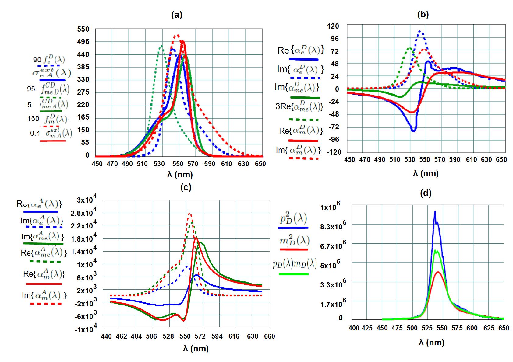
Figure A5 - 1: (Color online). Data of examples A and B: Both donor and acceptor are chiral and magnetoelectric. $n(\lambda)=1$. (a) Emission spectra in $fs$: $f_{e}^{D}(\lambda)$, $f_{m}^{D}(\lambda)$, $f_{me\,D}^{CD}(\lambda)$ of D, and extinction and dichroism cros-sections in $nm^{2}$: $\sigma_{e\,A}^{ext}(\lambda)$, $\sigma_{m\,A}^{ext}(\lambda)$, $\sigma_{me\,A}^{CD}(\lambda)$ of A. (b) Real and imaginary parts of the polarizabilities of D in $nm^{3}$: $\alpha_{e}^{D}(\lambda)$, $\alpha_{m}^{D}(\lambda)$ and $\alpha_{me}^{D}(\lambda)$. (c) Real and imaginary parts of the polarizabilities of A in $nm^{3}$: $\alpha_{e}^{A}(\lambda)$, $\alpha_{m}^{A}(\lambda)$ and $\alpha_{me}^{A}(\lambda)$. (d) Donor distributions: $p_{D}^{2}(\lambda)$, $m_{D}^{2}(\lambda)$ and $p_{D}(\lambda)m_{D}(\lambda)$ in arbitrary units for incident elliptic polarization with $e_{i}^{+}=7$, $e_{i}^{-}=3$ on D. The wavelength $\lambda$ is in $nm$.

Appendix E Appendix 5: Data for examples A and B: RHELT and RET when both donor and acceptor are chiral and magnetoelectric

Fig. A5-1(a) shows the spectra of the emission distributions of D, as well as extinction and CD cross-sections of A according to Eqs. (A3-1) and (A3-2). $n(\lambda)=1$ and $c=300nm\times fs^{-1}$. The polarizabilities of D and A, along with the products of the induced donor dipoles $p_{D}^{2}$, $m_{D}^{2}$ and $p_{D}m_{D}$ for incident elliptic polarization with $e_{i}^{+}=7$, $e_{i}^{-}=3$ on D, are shown in Fig. A5-1(b), (c) and (d), respectively.

We have chosen the lineshapes for the donor emission distributions of Eq. (A3-1) with

$D_{e}^{(1)}=3.91fs$, $D_{e}^{(2)}=1.86fs$, $\lambda_{e}^{(1)\,D}=542nm$, $\lambda_{e}^{(2)\,D}=560nm$, $\Delta\lambda_{e}^{(1)\,D}=11nm$, $\Delta\lambda_{e}^{(2)\,D}=29nm$, $D_{m}^{(1)}=2.18fs$, $D_{m}^{(2)}=1.52fs$, $\lambda_{m}^{(1)\,D}=546nm$, $\lambda_{m}^{(2)\,D}=561nm$, $\Delta\lambda_{m}^{(1)\,D}=15nm$, $\Delta\lambda_{m}^{(2)\,D}=39nm$, $D_{me}^{(1)}=3.75fs$, $D_{me}^{(2)}=1.54fs$, $\lambda_{me}^{(1)\,D}=528nm$, $\lambda_{me}^{(2)\,D}=562nm$, $\Delta\lambda_{me}^{(1)\,D}=12nm$, $\Delta\lambda_{me}^{(2)\,D}=26nm$.

Whereas for the magnetoelectric acceptor,[cf. Eq.(A3-2)], the parameters are:

$A_{e}^{(1)}=310nm^{2}$, $A_{e}^{(2)}=180nm^{2}$, $\lambda_{e}^{(1)\,A}=552.1nm$, $\lambda_{e}^{(2)\,A}=534.3nm$, $\Delta\lambda_{e}^{(1)\,A}=11.7nm$, $\Delta\lambda_{e}^{(2)\,A}=28.5nm$ $A_{m}^{(1)}=910nm^{2}$, $A_{m}^{(2)}=480nm^{2}$, $\lambda_{m}^{(1)\,A}=555.2nm$, $\lambda_{m}^{(2)\,A}=539.1nm$, $\Delta\lambda_{m}^{(1)\,A}=8.1nm$, $\Delta\lambda_{m}^{(2)\,A}=26.2nm$, $A_{me}^{(1)}=71nm^{2}$, $A_{me}^{(2)}=32nm^{2}$, $\lambda_{me}^{(1)\,A}=558.1nm$, $\lambda_{me}^{(2)\,A}=534.3nm$, $\Delta\lambda_{me}^{(1)\,A}=11.7nm$, $\Delta\lambda_{me}^{(2)\,A}=28.5nm$.

References

- (1) L. Allen, S. M. Barnett and M. J. Padgett, eds, Optical Angular Momentum, (IOP Publishing, Bristol, UK, 2003).
- (2) D. L. Andrews and M. Babiker, eds., The Angular Momentum of Light (Cambridge University press, Cambridge, 2013).
- (3) M. Yao and M. Padgett, Adv. Opt. Photon. 3, 161 (2011).
- (4) D. L. Andrews, M. M. Coles, M. D. Williams, and D. S. Bradshaw, Proc. SPIE 8813, 88130Y (2013).
- (5) M. N. O’Sullivan, M. Mirhosseini, M. Malik, and R. W. Boyd, , Opt. Express 20, 24444 (2012).
- (6) J. A. Schellman, Chem. Rev. 75, 323 (1975).
- (7) F. S. Richardson, and J. P. Riehl, Chem. Rev.77, 773 (1977).
- (8) L. Vuong, A. Adam, J. Brok, P. Planken, and H. Urbach, Phys. Rev. Lett. 104, 083903 (2010).
- (9) K. Y. Bliokh, F. Rodriguez-Fortuño, F. Nori, and A. V. Zayats, Nat. Photonics 9, 796 (2015).
- (10) S. Sukhov, V. Kajorndejnukul, R. R. Naraghi, and A. Dogariu, Nat. Photonics 9, 809 (2015).
- (11) D. Hakobyan, and E. Brasselet, Opt. Express 23, 31230 (2015).
- (12) K. Y. Bliokh, D. Smirnova, and F. Nori, Science 348, 1448 (2015).
- (13) D. S. Bradshaw, J. M. Leeder, M. M. Coles, and D.L. Andrews, Chem. Phys. Lett. 626, 106 (2015).
- (14) M. Nieto-Vesperinas, J. Opt. 19, 065402 (2017).
- (15) K. Y. Bliokh, Y. S. Kivshar, and F. Nori, Phys. Rev. Lett. 113, 033601 (2014).
- (16) A. Krasnok, S. Glybovski, M. Petrov, S. Makarov, R. Savelev, P. Belov, C. Simovski and Y.S. Kivshar, Appl. Phys. Lett. 108, 211 (2016.). (doi:10.1063/1.4952740).
- (17) Y. Tang, and A. E. Cohen, Phys. Rev. Lett. 104, 163901 (2010).
- (18) K.Y. Bliokh and F. Nori, Phys. Rev. A 83, 021803 (2011).
- (19) K. Y. Bliokh, A. Y. Bekshaev and F. Nori, New. J. Phys. 15 033026 (2013).
- (20) R. P. Cameron, S. M. Barnett and A. M. Yao, New J. Phys. 14, 053050 (2012).
- (21) R. P. Cameron and S. M. Barnett, New J. Phys. 14, 123019 (2012).
- (22) M. Nieto-Vesperinas, Phys. Rev. A 92, 023813 (2015).
- (23) M. Nieto-Vesperinas, Phil. Trans. R. Soc. A 375, 20160314 (2017).
- (24) P. Gutsche, P. I. Schneider, S. Burger and M. Nieto-Vesperinas, IOP Conf. Series: Journal of Physics 963, 012004 (2018). arXiv:1712.07091 (2018).
- (25) P. Gutsche, L. V. Poulikakos, M. Hammerschmidt, S. Burger. and F. Schmidt, Proc. SPIE 9756, 97560X arXiv:1603.05011 (2016).
- (26) L. V. Poulikakos, P. Gutsche, K. M. McPeak, S. Burger, J. Niegemann, C. Hafner and D. J. Norris, ACS Photonics 3 1619–25 (2016).
- (27) I. Fernandez-Corbaton and G. Molina-Terriza, Phys. Rev. B 88, 085111 (2013).
- (28) X. Zambrana-Puyalto and N. Bonod, Nanoscale 8, 10441 (2016).
- (29) P. Gutsche and M. Nieto-Vesperinas, Sci. Reps. 8 9416 (2018). DOI:10.1038/s41598-018-27496-w.
- (30) Y. Tang, Y. and A. E. Cohen, Science 332, 333 (2011).
- (31) N. Yang, Y. Tang, A. E. Cohen, Nano Today 4, 269, (2009)
- (32) J. S. Choi and M. Cho, Phys. Rev. A 86, 063834 (2012).
- (33) D. V. Guzatov and V. V. Klimov, New J. Phys. 14, 123009 (2012).
- (34) H. Alaeian, and J. A. Dionne, Phys. Rev. B 91, 245108 (2015).
- (35) M. Schäferling, D. Dregely, M. Hentschel and H. Giessen, Phys. Rev. X 2, 031010 (2012).
- (36) M. Hentschel, M. Schäferling, X. Duan, H. Giessen, and N. Liu, Chiral plasmonics. Sci. Adv. 3, e1602735 (2017).
- (37) C. Kramer, M. Schäferling, T. Weiss, H. Giessen, and M. Brixner, ACS Photonics 4, 396 (2017).
- (38) A. Garcia-Etxarri, A. and J. A. Dionne, Phys. Rev. B 87, 235409 (2013).
- (39) H. Wang, Z. Li, H. Zhang, P. Wang and S. Wen, Sci. Rep. 5, 8207 (2015).
- (40) R. Vincent, and R. Carminati, Phys. Rev. B 83, 165426 (2011).
- (41) L. Hu, X. Tian, Y.Huang, L. Fang and T. Fang, Nanoscale 8, 3720 (2016).
- (42) T. Förster, in Modern Quantum Chemistry, ed. O. Sinanoglu, (Academic P., New York 1965), pp. 93-137.
- (43) L. Stryer and R.P Haugland, Proc. Natl. Acad. Sci. USA 58 719 (1967).
- (44) J, P. Riehl and G. Muller, Circularly polarized luminescence spectroscopy and emission detected dichroism Chapt. 3, pp 64 of: Comprehensive spectroscopy. Vol. 1, N. Berova, P. L. Polavarapu, K. Nakanishi and R. W. Woody. J. Wiley, Hoboken, New Jersey 2012.
- (45) F. S. Richardson and J. P. Riehl, Circularly Polarized Luminescence Spectroscopy, Chem. Rev. 77 773 (1977).
- (46) C. R. Kagan, C. B. Murray, M. Nirmal, and M. G. Bawendi, Phys. Rev. Lett. 76, 1517 (1996).
- (47) R. M. Clegg, Förster resonance energy transfer—FRET. what is it, why do it, and how it’s done, Ch.1 of ”FRET and FLIM techniques”, T.W.J. Gadella, ed., Laboratory Techniques in Biochemistry and Molecular Biology 33, 1, (Academic Press, 2009).
- (48) L. Novotny L Hand B. Hecht, Principles of nano-optics, 2nd edn. Cambridge, UK: Cambridge University Press (2012).
- (49) D. P. Craig and T. Thirunamachandran, Chem. Phys. 167, 229 (1992)
- (50) A. Salam, Mol. Phys. 87 919 (1996).
- (51) D. P. Craig and T. Thirunamachandran, Theor. Chem. Acc. 102 112 (1999). DOI 10.1007/s00214980m157.
- (52) A. Salam, AIP Conference Proceedings 1642, 90 (2015); doi: 10.1063/1.4906634.
- (53) S. J. Leavesley and T. C. Rich, Cytometry A 89, 325 (2016).
- (54) M. Nieto-Vesperinas, R. Gomez-Medina, and J. J. Saenz, J. Opt. Soc. Am. A 28 54 (2011).
- (55) A. Garcia-Etxarri, R. Gomez-Medina, L.S. Froufe-Perez, C. Lopez, L. Chantada, F. Scheffold, J. Aizpurua, M. Nieto-Vesperinas and J.J. Saenz, Opt. Express 19, 4815 (2011).
- (56) J. M. Geffrin, B. Garcia-Camara, R. Gomez-Medina, P. Albella, L. S. Froufe-Perez, C. Eyraud, A. Litman, R. Vaillon, F. Gonzalez, M. Nieto-Vesperinas, J. J. Saenz and F. Moreno, Nat. Commun. 3 1171 (2012).
- (57) A. I. Kuznetsov, A. E. Miroshnichenko, Y. H. Fu, J. Zhang and B. Luk’yanchuk, Sci. Reps. 2, 492 (2012).
- (58) M. Decker and I. Staude, J. Opt. 18, 103001 (2016) .
- (59) A. I. Kuznetsov, A. E. Miroshnichenko, M. L. Brongersma,Y. S. Kivshar, B. Luk’yanchuk, Science 354 (2016) 2472.
- (60) M. Nieto-Vesperinas, Opt. Lett. 40, 3021 (2015).
- (61) A. Madrazo, M.Nieto-Vesperinas and N. Garcia, Phys. Rev. B 53, 3654 (1996).
- (62) M. Nieto-Vesperinas and N. Garcia, (eds), Optics at the Nanometer Scale: Imaging and Storing with Photonic Near Fields, NATO ASI Series, E-319, (Springer, 1996. Reprinted: 2012).
- (63) J. Kumar, T. Nakashima and T. Kawai, J. Phys. Chem. Lett. 6, 3445 (2015).
- (64) W. Yan, L. Xu, Ch. Xu, W. Ma, H. Kuang, L. Wang and N. A. Kotov, J. Am. Chem. Soc. 134, 15114 (2012).
- (65) P. Haro-Gonzalez, B. del Rosal a L. M. Maestro, E. Martin Rodriguez, R. Naccache, J. A. Capobianco, K. Dholakia, J. Garciıa Solea and D. Jaque, Nanoscale 5, 12192 (2013).
- (66) A. Lay, D. S. Wang, M. D. Wisser, R. D. Mehlenbacher, Y. Lin, M. B. Goodman, W. L. Mao and J. A. Dionne, Nano Lett. 17, 4172 (2017).
- (67) S. Wen, J. Zhou, K. Zheng, A. Bednarkiewicz, X. Liu and D. Jin, Nat. Comm. 9, 2415 (2018).
- (68) I.V. Lindell and A. Shivola, Electromagnetic waves in chiral and bi-isotropic media, Artech House, London, 1994.
- (69) C. Berney and G. Danuser, Biophys. J. 84, 3992 (2003).
- (70) A. Canaguier-Durand, J. A Hutchison, C. Genet and T. W. Ebbesen, New J. Phys. 15, 123037 (2013).
- (71) M. Born and E. Wolf, Principles of Optics, 7 th edition, Cambridge U.P., Cambridge, 1999.
- (72) S. Nechayev, S. Eismann, G. Leuchs and P. Banzer, Phys Rev. B 99, 075155 (2019); S. Nechayev and P. Banzer, Phys. Rev. B 99, 241101(R) (2019).
- (73) M. Nieto-Vesperinas, J. J. Saenz, R. Gomez-Medina and L. Chantada, Opt. Exp. 18, 11428 (2010).
- (74) L. D. Barron,Molecular Light Scattering and Optical Activity, (Cambridge U.P., Cambridge, 2004).