Rotor walks on transient graphs and the wired spanning forest

Abstract.

We study rotor walks on transient graphs with initial rotor configuration sampled from the oriented wired uniform spanning forest (OWUSF) measure. We show that the expected number of visits to any vertex by the rotor walk is at most equal to the expected number of visits by the simple random walk. In particular, this implies that this walk is transient. When these two numbers coincide, we show that the rotor configuration at the end of the process also has the law of OWUSF. Furthermore, if the graph is vertex-transitive, we show that the average number of visits by $n$ consecutive rotor walks converges to the Green function of the simple random walk as $n$ tends to infinity. This answers a question posed by Florescu, Ganguly, Levine, and Peres (2014).

1. Introduction

In a rotor walk [WLB96, PDDK96, Pro03] on a graph $G$, each vertex is assigned a fixed cyclic ordering of its neighbors, and each vertex has a rotor, which is an arrow that points to one of its neighbors. A rotor configuration is an assignment of directions to all the rotors. Given an initial rotor configuration, a walker (initially located at a fixed vertex) explores the graph using the following rule: at each time step, the walker changes the rotor of its current location to point to the next neighbor given by the cyclic ordering, and then the walker moves to this new neighbor. The rotor walk is obtained by repeated applications of this rule.

One major difference of this paper compared to other works in the literature is our choice of initial rotor configuration; it is sampled from the oriented wired uniform spanning forest measure. Let $G$ be a connected graph that is simple (i.e. no loops or multiple edges), transient, and locally finite (i.e. every vertex has finite degree), and let $W_{1}\subseteq W_{2}\subseteq\ldots$ be finite connected subsets of $V(G)$ such that $\bigcup_{R=1}^{\infty}W_{R}=V(G)$. Let $G_{R}$ be obtained from $G$ by identifying all vertices outside $W_{R}$ to one new vertex $w_{R}$, and let $\mu_{R}$ be the uniform measure on spanning trees of $G_{R}$ oriented toward $w_{R}$. Then $\mu_{R}$ has a unique infinite volume limit [Pem91, BLPS01], which we call the wired spanning forest oriented toward infinity $\operatorname{\mathchoice{\vbox{\halign{#\cr\arrowfill@\relbar\relbar\rightharpoonup{\scriptstyle}\crcr\nointerlineskip\cr$\hfil\displaystyle\mathsf{WUSF}\hfil$\crcr}}}{\vbox{\halign{#\cr\arrowfill@\relbar\relbar\rightharpoonup{\scriptstyle}\crcr\nointerlineskip\cr$\hfil\textstyle\mathsf{WUSF}\hfil$\crcr}}}{\vbox{\halign{#\cr\arrowfill@\relbar\relbar\rightharpoonup{\scriptscriptstyle}\crcr\nointerlineskip\cr$\hfil\scriptstyle\mathsf{WUSF}\hfil$\crcr}}}{\vbox{\halign{#\cr\arrowfill@\relbar\relbar\rightharpoonup{\scriptscriptstyle}\crcr\nointerlineskip\cr$\hfil\scriptscriptstyle\mathsf{WUSF}\hfil$\crcr}}}}(G)$. See [BLPS01, LP16] for more details.

Several studies had been conducted to compare the behavior of rotor walks to the expected behavior of simple random walks (e.g.[CDST06, CS06, LL09, LP09, HMSH15, HS18]). One such result is due to Schramm [HP10, Theorem 10], who showed that the rotor walk is in a certain sense at most as transient as the simple random walk. We will show that that the opposite is true when the initial rotor configuration is given by $\operatorname{\mathchoice{\vbox{\halign{#\cr\arrowfill@\relbar\relbar\rightharpoonup{\scriptstyle}\crcr\nointerlineskip\cr$\hfil\displaystyle\mathsf{WUSF}\hfil$\crcr}}}{\vbox{\halign{#\cr\arrowfill@\relbar\relbar\rightharpoonup{\scriptstyle}\crcr\nointerlineskip\cr$\hfil\textstyle\mathsf{WUSF}\hfil$\crcr}}}{\vbox{\halign{#\cr\arrowfill@\relbar\relbar\rightharpoonup{\scriptscriptstyle}\crcr\nointerlineskip\cr$\hfil\scriptstyle\mathsf{WUSF}\hfil$\crcr}}}{\vbox{\halign{#\cr\arrowfill@\relbar\relbar\rightharpoonup{\scriptscriptstyle}\crcr\nointerlineskip\cr$\hfil\scriptscriptstyle\mathsf{WUSF}\hfil$\crcr}}}}(G)$, in a manner to be made precise.

One way to measure the transience of rotor walks is to count the number of visits to any vertex. Fix a vertex $a$ as the initial location of the walker. Let $u(\rho,x)$ be the number of visits to $x\in V(G)$ by the rotor walk with initial rotor configuration $\rho$, and let $\operatorname{\mathcal{G}}(x)$ be the expected number of visits to $x$ by the simple random walk. Note that $\operatorname{\mathcal{G}}(x)$ is finite since the graph $G$ is transient.

Theorem 1.1.

Let $G$ be a simple connected graph that is locally finite and transient. Consider any rotor walk on $G$ with the walker initially located at a fixed vertex $a$. Then,

$$\operatorname{\mathbb{E}}_{\rho}[u(\rho,x)]\leq\operatorname{\mathcal{G}}(x)\qquad\forall\ x\in V(G),$$ (1)

where $\rho$ is sampled from $\operatorname{\mathchoice{\vbox{\halign{#\cr\arrowfill@\relbar\relbar\rightharpoonup{\scriptstyle}\crcr\nointerlineskip\cr$\hfil\displaystyle\mathsf{WUSF}\hfil$\crcr}}}{\vbox{\halign{#\cr\arrowfill@\relbar\relbar\rightharpoonup{\scriptstyle}\crcr\nointerlineskip\cr$\hfil\textstyle\mathsf{WUSF}\hfil$\crcr}}}{\vbox{\halign{#\cr\arrowfill@\relbar\relbar\rightharpoonup{\scriptscriptstyle}\crcr\nointerlineskip\cr$\hfil\scriptstyle\mathsf{WUSF}\hfil$\crcr}}}{\vbox{\halign{#\cr\arrowfill@\relbar\relbar\rightharpoonup{\scriptscriptstyle}\crcr\nointerlineskip\cr$\hfil\scriptscriptstyle\mathsf{WUSF}\hfil$\crcr}}}}(G)$.

We prove Theorem 1.1 by first proving an analogous statement for finite graphs, and the statement for infinite graphs then follows by taking the infinite volume limit.

One consequence of Theorem 1.1 is that the rotor walk with initial rotor configuration picked from $\operatorname{\mathchoice{\vbox{\halign{#\cr\arrowfill@\relbar\relbar\rightharpoonup{\scriptstyle}\crcr\nointerlineskip\cr$\hfil\displaystyle\mathsf{WUSF}\hfil$\crcr}}}{\vbox{\halign{#\cr\arrowfill@\relbar\relbar\rightharpoonup{\scriptstyle}\crcr\nointerlineskip\cr$\hfil\textstyle\mathsf{WUSF}\hfil$\crcr}}}{\vbox{\halign{#\cr\arrowfill@\relbar\relbar\rightharpoonup{\scriptscriptstyle}\crcr\nointerlineskip\cr$\hfil\scriptstyle\mathsf{WUSF}\hfil$\crcr}}}{\vbox{\halign{#\cr\arrowfill@\relbar\relbar\rightharpoonup{\scriptscriptstyle}\crcr\nointerlineskip\cr$\hfil\scriptscriptstyle\mathsf{WUSF}\hfil$\crcr}}}}(G)$ is transient (i.e., every vertex is visited only finitely many times) almost surely. We remark that the rotor walk with an arbitrary initial rotor configuration can fail to be transient even if the underlying graph is transient; see [AH12, Theorem 2].

Note that the inequality in (1) can be strict, as shown in Figure 1 with $G$ being a transient tree with an extra infinite path attached to the root. Somewhat surprisingly, having equality in (1) turns out to have the following interesting implication.

(a)

(b)

(c)

Figure 1. (a) The $2$-ary tree with an extra infinite path attached to its root. (b) An initial rotor configuration $\rho$ sampled from $\operatorname{\mathchoice{\vbox{\halign{#\cr\arrowfill@\relbar\relbar\rightharpoonup{\scriptstyle}\crcr\nointerlineskip\cr$\hfil\displaystyle\mathsf{WUSF}\hfil$\crcr}}}{\vbox{\halign{#\cr\arrowfill@\relbar\relbar\rightharpoonup{\scriptstyle}\crcr\nointerlineskip\cr$\hfil\textstyle\mathsf{WUSF}\hfil$\crcr}}}{\vbox{\halign{#\cr\arrowfill@\relbar\relbar\rightharpoonup{\scriptscriptstyle}\crcr\nointerlineskip\cr$\hfil\scriptstyle\mathsf{WUSF}\hfil$\crcr}}}{\vbox{\halign{#\cr\arrowfill@\relbar\relbar\rightharpoonup{\scriptscriptstyle}\crcr\nointerlineskip\cr$\hfil\scriptscriptstyle\mathsf{WUSF}\hfil$\crcr}}}}(G)$, and a walker at the initial location $a$, marked with a (blue) bullet. The rotors of $\rho$ in the extra infinite path form a path oriented toward $a$ almost surely by Wilson’s method [BLPS01]. (c) The final rotor configuration $\sigma(\rho)$ after the rotor walk is performed. The number of visits $u(\rho,a)$ to $a$ is equal to 1 almost surely as $a$ is visited only once (i.e., at the beginning at the walk), while the Green function $\operatorname{\mathcal{G}}(a)$ is equal to $3$ (see [LP16, Exercise 2.8]). Furthermore, $\rho$ and $\sigma(\rho)$ follow different laws as the former has an infinite path oriented toward $a$ almost surely while the latter has the same path oriented outward of $a$ almost surely.

Let $\rho$ be a rotor configuration such that the corresponding rotor walk is transient. Then the final rotor configuration $\sigma(\rho)$ is given by $\sigma(\rho)(x):=\lim_{t\to\infty}\rho_{t}(x)$. Here $\rho_{t}$ denotes the rotor configuration at the $t$-th step of the rotor walk. Note that the limit $\lim_{t\to\infty}\rho_{t}(x)$ exists as the sequence is eventually constant. A probability measure $\mu$ on rotor configurations is stationary with respect to the rotor walk if $\rho\overset{d}{=}\mu$ implies $\sigma(\rho)\overset{d}{=}\mu$.

Theorem 1.2.

Let $G$ be a simple connected graph that is locally finite and transient. Consider any rotor walk on $G$ with the walker initially located at a fixed vertex $a$. Let $\rho$ be sampled from $\operatorname{\mathchoice{\vbox{\halign{#\cr\arrowfill@\relbar\relbar\rightharpoonup{\scriptstyle}\crcr\nointerlineskip\cr$\hfil\displaystyle\mathsf{WUSF}\hfil$\crcr}}}{\vbox{\halign{#\cr\arrowfill@\relbar\relbar\rightharpoonup{\scriptstyle}\crcr\nointerlineskip\cr$\hfil\textstyle\mathsf{WUSF}\hfil$\crcr}}}{\vbox{\halign{#\cr\arrowfill@\relbar\relbar\rightharpoonup{\scriptscriptstyle}\crcr\nointerlineskip\cr$\hfil\scriptstyle\mathsf{WUSF}\hfil$\crcr}}}{\vbox{\halign{#\cr\arrowfill@\relbar\relbar\rightharpoonup{\scriptscriptstyle}\crcr\nointerlineskip\cr$\hfil\scriptscriptstyle\mathsf{WUSF}\hfil$\crcr}}}}(G)$. Then, the following are equivalent:

1. $\operatorname{\mathchoice{\vbox{\halign{#\cr\arrowfill@\relbar\relbar\rightharpoonup{\scriptstyle}\crcr\nointerlineskip\cr$\hfil\displaystyle\mathsf{WUSF}\hfil$\crcr}}}{\vbox{\halign{#\cr\arrowfill@\relbar\relbar\rightharpoonup{\scriptstyle}\crcr\nointerlineskip\cr$\hfil\textstyle\mathsf{WUSF}\hfil$\crcr}}}{\vbox{\halign{#\cr\arrowfill@\relbar\relbar\rightharpoonup{\scriptscriptstyle}\crcr\nointerlineskip\cr$\hfil\scriptstyle\mathsf{WUSF}\hfil$\crcr}}}{\vbox{\halign{#\cr\arrowfill@\relbar\relbar\rightharpoonup{\scriptscriptstyle}\crcr\nointerlineskip\cr$\hfil\scriptscriptstyle\mathsf{WUSF}\hfil$\crcr}}}}(G)$ is stationary with respect to the rotor walk;

2. We have $\operatorname{\mathbb{E}}_{\rho}[u(\rho,x)]=\operatorname{\mathcal{G}}(x)$ for all $x\in V(G)$.

The proof of Theorem 1.2 uses an idea similar to Theorem 1.1; we first show an analogous statement for the finite graphs, and then we take the infinite volume limit. This limit needs to be taken over a sequence of random variables that are tight (as otherwise the equality in (ii) will we weakened to an inequality), and this tightness condition turns out to be equivalent to requiring the stationarity of $\operatorname{\mathchoice{\vbox{\halign{#\cr\arrowfill@\relbar\relbar\rightharpoonup{\scriptstyle}\crcr\nointerlineskip\cr$\hfil\displaystyle\mathsf{WUSF}\hfil$\crcr}}}{\vbox{\halign{#\cr\arrowfill@\relbar\relbar\rightharpoonup{\scriptstyle}\crcr\nointerlineskip\cr$\hfil\textstyle\mathsf{WUSF}\hfil$\crcr}}}{\vbox{\halign{#\cr\arrowfill@\relbar\relbar\rightharpoonup{\scriptscriptstyle}\crcr\nointerlineskip\cr$\hfil\scriptstyle\mathsf{WUSF}\hfil$\crcr}}}{\vbox{\halign{#\cr\arrowfill@\relbar\relbar\rightharpoonup{\scriptscriptstyle}\crcr\nointerlineskip\cr$\hfil\scriptscriptstyle\mathsf{WUSF}\hfil$\crcr}}}}(G)$. A more detailed sketch is provided in Section 6.

See Proposition 7.1 for graphs for which $\operatorname{\mathchoice{\vbox{\halign{#\cr\arrowfill@\relbar\relbar\rightharpoonup{\scriptstyle}\crcr\nointerlineskip\cr$\hfil\displaystyle\mathsf{WUSF}\hfil$\crcr}}}{\vbox{\halign{#\cr\arrowfill@\relbar\relbar\rightharpoonup{\scriptstyle}\crcr\nointerlineskip\cr$\hfil\textstyle\mathsf{WUSF}\hfil$\crcr}}}{\vbox{\halign{#\cr\arrowfill@\relbar\relbar\rightharpoonup{\scriptscriptstyle}\crcr\nointerlineskip\cr$\hfil\scriptstyle\mathsf{WUSF}\hfil$\crcr}}}{\vbox{\halign{#\cr\arrowfill@\relbar\relbar\rightharpoonup{\scriptscriptstyle}\crcr\nointerlineskip\cr$\hfil\scriptscriptstyle\mathsf{WUSF}\hfil$\crcr}}}}(G)$ is stationary with respect to the rotor walk. Those examples include the $b$-ary tree $\operatorname{\mathbb{T}}_{b}$ for $b\geq 2$ (i.e. a tree with a root vertex $o$ having degree $b$ and with every other vertex having degree $b+1$). For the other end of the spectrum, see Figure 1 for a graph for which $\operatorname{\mathchoice{\vbox{\halign{#\cr\arrowfill@\relbar\relbar\rightharpoonup{\scriptstyle}\crcr\nointerlineskip\cr$\hfil\displaystyle\mathsf{WUSF}\hfil$\crcr}}}{\vbox{\halign{#\cr\arrowfill@\relbar\relbar\rightharpoonup{\scriptstyle}\crcr\nointerlineskip\cr$\hfil\textstyle\mathsf{WUSF}\hfil$\crcr}}}{\vbox{\halign{#\cr\arrowfill@\relbar\relbar\rightharpoonup{\scriptscriptstyle}\crcr\nointerlineskip\cr$\hfil\scriptstyle\mathsf{WUSF}\hfil$\crcr}}}{\vbox{\halign{#\cr\arrowfill@\relbar\relbar\rightharpoonup{\scriptscriptstyle}\crcr\nointerlineskip\cr$\hfil\scriptscriptstyle\mathsf{WUSF}\hfil$\crcr}}}}(G)$ is not stationary. We remark that the stationarity of $\operatorname{\mathchoice{\vbox{\halign{#\cr\arrowfill@\relbar\relbar\rightharpoonup{\scriptstyle}\crcr\nointerlineskip\cr$\hfil\displaystyle\mathsf{WUSF}\hfil$\crcr}}}{\vbox{\halign{#\cr\arrowfill@\relbar\relbar\rightharpoonup{\scriptstyle}\crcr\nointerlineskip\cr$\hfil\textstyle\mathsf{WUSF}\hfil$\crcr}}}{\vbox{\halign{#\cr\arrowfill@\relbar\relbar\rightharpoonup{\scriptscriptstyle}\crcr\nointerlineskip\cr$\hfil\scriptstyle\mathsf{WUSF}\hfil$\crcr}}}{\vbox{\halign{#\cr\arrowfill@\relbar\relbar\rightharpoonup{\scriptscriptstyle}\crcr\nointerlineskip\cr$\hfil\scriptscriptstyle\mathsf{WUSF}\hfil$\crcr}}}}(\operatorname{\mathbb{Z}}^{d})$ for rotor walks on $\operatorname{\mathbb{Z}}^{d}$ ($d\geq 3$) remains an open problem; see Section 9.

Another way to measure the transience of rotor walks is the following method introduced by Florescu, Ganguly, Levine, and Peres (FGLP) [FGLP14]: Start with an initial rotor configuration and with $n$ walkers located at the fixed vertex $a$. Let each of these $n$ walkers in turn perform rotor walk (note that we do not reset the rotors in between runs!). Let $S_{n}(\rho,x)$ be equal to the total number of visits to $x$ by all the walkers if all of the $n$ rotor walks are transient, and is equal to infinity otherwise. The occupation rate $S_{n}(\rho,x)/n$ satisfies the following inequality,

$$\liminf_{n\to\infty}\frac{S_{n}(\rho,x)}{n}\geq\operatorname{\mathcal{G}}(x).$$ (2)

The proof of (2) for when $x$ is equal to the initial vertex $a$ is due to Schramm (see [HP10, Theorem 10] and [FGLP14, Section 2]). Note that Schramm stated (2) in terms of the escape rate of the rotor walk, which is inversely proportional to ${S_{n}(\rho,a)}/{n}$; see [FGLP14, Lemma 5]. We include a proof of (2) in this paper for completeness; see Lemma 5.1.

The inequality in (2) can be strict; see [AH11, Theorem 2(iii)]. FGLP then asked for the next best thing: must there always exist a rotor configuration for which equality occurs in (2)? We give a positive answer to a weaker probabilistic variant of this question.

Theorem 1.3.

Let $G$ be a simple connected graph that is locally finite, transient, and vertex-transitive. Consider any rotor walk on $G$ with the walker initially located at a fixed vertex $a$. Let $\rho$ be sampled from $\operatorname{\mathchoice{\vbox{\halign{#\cr\arrowfill@\relbar\relbar\rightharpoonup{\scriptstyle}\crcr\nointerlineskip\cr$\hfil\displaystyle\mathsf{WUSF}\hfil$\crcr}}}{\vbox{\halign{#\cr\arrowfill@\relbar\relbar\rightharpoonup{\scriptstyle}\crcr\nointerlineskip\cr$\hfil\textstyle\mathsf{WUSF}\hfil$\crcr}}}{\vbox{\halign{#\cr\arrowfill@\relbar\relbar\rightharpoonup{\scriptscriptstyle}\crcr\nointerlineskip\cr$\hfil\scriptstyle\mathsf{WUSF}\hfil$\crcr}}}{\vbox{\halign{#\cr\arrowfill@\relbar\relbar\rightharpoonup{\scriptscriptstyle}\crcr\nointerlineskip\cr$\hfil\scriptscriptstyle\mathsf{WUSF}\hfil$\crcr}}}}(G)$. Then occupation rates $S_{n}(\rho,x)/n$ converge in norm to $\operatorname{\mathcal{G}}(x)$, i.e.,

$$\lim_{n\to\infty}\operatorname{\mathbb{E}}_{\rho}\left[\left|\frac{S_{n}(\rho,x)}{n}-\operatorname{\mathcal{G}}(x)\right|\right]=0\qquad\forall x\in V(G).$$

The proof of Theorem 1.3 is derived from an upper bound for the expected value of occupation rates that holds if $\rho\overset{d}{=}\operatorname{\mathchoice{\vbox{\halign{#\cr\arrowfill@\relbar\relbar\rightharpoonup{\scriptstyle}\crcr\nointerlineskip\cr$\hfil\displaystyle\mathsf{WUSF}\hfil$\crcr}}}{\vbox{\halign{#\cr\arrowfill@\relbar\relbar\rightharpoonup{\scriptstyle}\crcr\nointerlineskip\cr$\hfil\textstyle\mathsf{WUSF}\hfil$\crcr}}}{\vbox{\halign{#\cr\arrowfill@\relbar\relbar\rightharpoonup{\scriptscriptstyle}\crcr\nointerlineskip\cr$\hfil\scriptstyle\mathsf{WUSF}\hfil$\crcr}}}{\vbox{\halign{#\cr\arrowfill@\relbar\relbar\rightharpoonup{\scriptscriptstyle}\crcr\nointerlineskip\cr$\hfil\scriptscriptstyle\mathsf{WUSF}\hfil$\crcr}}}}(G)$ and the lower bound for occupation rates from (2) that holds for any $\rho$.

When the underlying graph is vertex-transitive, we can upgrade the convergence in norm in Theorem 1.3 to the almost sure convergence and gives a positive answer to the question of FGLP.

Theorem 1.4.

Let $G$ be a simple connected graph that is locally finite, transient, and vertex-transitive. Consider any rotor walk on $G$ with the walker initially located at a fixed vertex $a$. Then, for almost every $\rho$ picked from $\operatorname{\mathchoice{\vbox{\halign{#\cr\arrowfill@\relbar\relbar\rightharpoonup{\scriptstyle}\crcr\nointerlineskip\cr$\hfil\displaystyle\mathsf{WUSF}\hfil$\crcr}}}{\vbox{\halign{#\cr\arrowfill@\relbar\relbar\rightharpoonup{\scriptstyle}\crcr\nointerlineskip\cr$\hfil\textstyle\mathsf{WUSF}\hfil$\crcr}}}{\vbox{\halign{#\cr\arrowfill@\relbar\relbar\rightharpoonup{\scriptscriptstyle}\crcr\nointerlineskip\cr$\hfil\scriptstyle\mathsf{WUSF}\hfil$\crcr}}}{\vbox{\halign{#\cr\arrowfill@\relbar\relbar\rightharpoonup{\scriptscriptstyle}\crcr\nointerlineskip\cr$\hfil\scriptscriptstyle\mathsf{WUSF}\hfil$\crcr}}}}(G)$,

$$\lim_{n\to\infty}\frac{S_{n}(\rho,x)}{n}=\operatorname{\mathcal{G}}(x)\qquad\forall\ x\in V(G).$$

The proof of Theorem 1.4 is inspired by Etemadi’s proof of strong law of large numbers [Ete81]. We first estimate the probability $q_{n}$ that $S_{n}/n$ differs from $\operatorname{\mathcal{G}}$ by more than $\epsilon$. We then show that the sum $\sum q_{n}$ is finite when summed over any subsequence $n_{1},n_{2},\ldots$ that grows exponentially, and by Borel-Cantelli lemma we then conclude that $S_{n}/n$ converges for these subsequences. We then upgrade this convergence to the whole sequence by using the inequality

$$\left(\frac{n_{k}}{n_{k+1}}\right)\frac{S_{n_{k}}}{n_{k}}\ \leq\ \frac{S_{n}}{n}\ \leq\ \left(\frac{n_{k+1}}{n_{k}}\right)\frac{S_{n_{k+1}}}{n_{k+1}},$$

which holds for any $n\in[n_{k},n_{k+1}]$ ($k\geq 1$).

The crucial step here is the estimate of $q_{n}$, which uses an upper bound for occupation rates that hold if $\rho\overset{d}{=}\operatorname{\mathchoice{\vbox{\halign{#\cr\arrowfill@\relbar\relbar\rightharpoonup{\scriptstyle}\crcr\nointerlineskip\cr$\hfil\displaystyle\mathsf{WUSF}\hfil$\crcr}}}{\vbox{\halign{#\cr\arrowfill@\relbar\relbar\rightharpoonup{\scriptstyle}\crcr\nointerlineskip\cr$\hfil\textstyle\mathsf{WUSF}\hfil$\crcr}}}{\vbox{\halign{#\cr\arrowfill@\relbar\relbar\rightharpoonup{\scriptscriptstyle}\crcr\nointerlineskip\cr$\hfil\scriptstyle\mathsf{WUSF}\hfil$\crcr}}}{\vbox{\halign{#\cr\arrowfill@\relbar\relbar\rightharpoonup{\scriptscriptstyle}\crcr\nointerlineskip\cr$\hfil\scriptscriptstyle\mathsf{WUSF}\hfil$\crcr}}}}(G)$ and a quantitative version of (2) that gives a lower bound for occupation rates in terms of the volume growth of $G$. The volume growth of $G$ can in turn be estimated by using the work [SC95, Tro03] that holds for all vertex-transitive graphs.

We now present another scenario for which we can give a positive answer to the question of FGLP.

Theorem 1.5.

Let $G$ be a connected simple graph that is locally finite and transient. Consider any rotor walk on $G$ with the walker initially located at a fixed vertex $a$. Suppose that $\operatorname{\mathchoice{\vbox{\halign{#\cr\arrowfill@\relbar\relbar\rightharpoonup{\scriptstyle}\crcr\nointerlineskip\cr$\hfil\displaystyle\mathsf{WUSF}\hfil$\crcr}}}{\vbox{\halign{#\cr\arrowfill@\relbar\relbar\rightharpoonup{\scriptstyle}\crcr\nointerlineskip\cr$\hfil\textstyle\mathsf{WUSF}\hfil$\crcr}}}{\vbox{\halign{#\cr\arrowfill@\relbar\relbar\rightharpoonup{\scriptscriptstyle}\crcr\nointerlineskip\cr$\hfil\scriptstyle\mathsf{WUSF}\hfil$\crcr}}}{\vbox{\halign{#\cr\arrowfill@\relbar\relbar\rightharpoonup{\scriptscriptstyle}\crcr\nointerlineskip\cr$\hfil\scriptscriptstyle\mathsf{WUSF}\hfil$\crcr}}}}(G)$ is stationary with respect to the given rotor walk. Then, for almost every $\rho$ picked from $\operatorname{\mathchoice{\vbox{\halign{#\cr\arrowfill@\relbar\relbar\rightharpoonup{\scriptstyle}\crcr\nointerlineskip\cr$\hfil\displaystyle\mathsf{WUSF}\hfil$\crcr}}}{\vbox{\halign{#\cr\arrowfill@\relbar\relbar\rightharpoonup{\scriptstyle}\crcr\nointerlineskip\cr$\hfil\textstyle\mathsf{WUSF}\hfil$\crcr}}}{\vbox{\halign{#\cr\arrowfill@\relbar\relbar\rightharpoonup{\scriptscriptstyle}\crcr\nointerlineskip\cr$\hfil\scriptstyle\mathsf{WUSF}\hfil$\crcr}}}{\vbox{\halign{#\cr\arrowfill@\relbar\relbar\rightharpoonup{\scriptscriptstyle}\crcr\nointerlineskip\cr$\hfil\scriptscriptstyle\mathsf{WUSF}\hfil$\crcr}}}}(G)$,

$$\lim_{n\to\infty}\frac{S_{n}(\rho,x)}{n}=\operatorname{\mathcal{G}}(x)\qquad\forall\ x\in V(G).$$

The proof of Theorem 1.5 uses the pointwise ergodic theorem to derive the almost sure convergence. Note that we can use the pointwise ergodic theorem because the initial rotor configuration is stationary with respect to the rotor walk.

The question of FGLP has previously been answered positively for all trees by Angel and Holroyd [AH11] and for $\operatorname{\mathbb{Z}}^{d}$ by He [He14]. In both cases, Theorem 1.4 (for $\operatorname{\mathbb{Z}}^{d}$) and Theorem 1.5 (for $\operatorname{\mathbb{T}}_{b}$) provide new examples of rotor configurations that answer the question of FGLP. For any other vertex-transitive graph, Theorem 1.4 is the first one to provide an answer to this question to the best of our knowledge.

This paper is structured as follows. In Section 2 we review notations for rotor walks that will be used throughout this paper. In Section 3 we review basic results for rotor walks on finite graphs. In Section 4 we prove Theorem 1.1. In Section 5 we prove Theorem 1.3. In Section 6 we prove Theorem 1.2. In Section 7 we provide some examples of graphs for which $\operatorname{\mathchoice{\vbox{\halign{#\cr\arrowfill@\relbar\relbar\rightharpoonup{\scriptstyle}\crcr\nointerlineskip\cr$\hfil\displaystyle\mathsf{WUSF}\hfil$\crcr}}}{\vbox{\halign{#\cr\arrowfill@\relbar\relbar\rightharpoonup{\scriptstyle}\crcr\nointerlineskip\cr$\hfil\textstyle\mathsf{WUSF}\hfil$\crcr}}}{\vbox{\halign{#\cr\arrowfill@\relbar\relbar\rightharpoonup{\scriptscriptstyle}\crcr\nointerlineskip\cr$\hfil\scriptstyle\mathsf{WUSF}\hfil$\crcr}}}{\vbox{\halign{#\cr\arrowfill@\relbar\relbar\rightharpoonup{\scriptscriptstyle}\crcr\nointerlineskip\cr$\hfil\scriptscriptstyle\mathsf{WUSF}\hfil$\crcr}}}}(G)$ is stationary with respect to the rotor walk. In Section 8 we prove Theorem 1.4 and Theorem 1.5. In Section 9 we list some open problems.

Remark.

Most of our results hold for the more general setting of random walks with local memory (RWLM) [CGLL18], where the update step for the rotor at any vertex $x$ is determined by a Markov chain $M_{x}$ assigned to $x$ (instead of the given cyclic ordering). Here $M_{x}$ is an ergodic Markov chain such that its state space is the neighbors $N(x)$ of $x$ and its stationary distribution is the uniform distribution on $N(x)$. In particular, Theorem 1.1, 1.2, 1.3, and 1.5 hold for all RWLMs. Note that Theorem 1.4 does not immediately extend to all RWLMs as the estimate of $q_{n}$ used in the proof is exclusive to rotor walks.

2. Preliminaries

Throughout this paper $G:=(V(G),E(G))$ is a connected simple undirected graph that is locally finite (i.e. every vertex has finitely many edges).

The rotor walk $(X_{t})_{t\geq 0}$ on $G$ is defined as follows. Fix a vertex $a\in V(G)$ and a subset $Z\subseteq V(G)$. To each vertex $x\in V(G)\setminus Z$ we assign a local mechanism $\tau_{x}$, which is a bijection on the neighbors $N(x)$ of $x$. We assume that each $\tau_{x}$ has one unique orbit (i.e. $\{\tau^{i}(y)\mid i\geq 0\}=N(x)$ for any neighbor $y$ of $x$). A rotor configuration of $G$ is a function $\rho:V(G)\setminus Z\to V(G)$ such that $\rho(x)\in N(x)$ for all $x\in V(G)\setminus Z$.

The walker is initially located at $a$ (i.e. $X_{0}:=a$) and with an initial rotor configuration $\rho_{0}:=\rho$. At the $t$-th step of the walk, the rotor of the current location of the walker is incremented to point to the next vertex in the cyclic order specified by its local mechanism, and then the walker moves to the vertex specified by this new rotor. That is to say,

$$\begin{split}\rho_{t+1}(x)&:=\begin{cases}\rho_{t}(x)&\text{ if }x\neq X_{t};\\ \tau_{X_{t}}(\rho_{t}(X_{t}))&\text{ if }x=X_{t},\end{cases}\\ X_{t+1}&:=\tau_{X_{t}}(\rho_{t}(X_{t})).\end{split}$$ (3)

The walk is immediately terminated if the walker reaches a vertex in the sink $Z$. Note that it is possible for a walk to never terminate.

A rotor walk is transient if every vertex of $G$ is visited by the walker at most finitely many times, and is recurrent otherwise.

One aspect of the rotor walk that we will study in this paper is the final rotor configuration of a transient walk, defined as follows.

Definition 2.1 (Final rotor configuration).

The final rotor configuration $\sigma(\rho):=\sigma_{G,Z}(a,\rho)$ of a transient rotor walk is given by

$$\sigma(\rho)(x):=\lim_{t\to\infty}\rho_{t}(x)\qquad\forall x\in V(G).\qed$$

Note that $\sigma(\rho)$ is well defined as the sequence $(\rho_{t}(x))_{t\geq 0}$ is eventually constant by the assumption that the walk is transient.

Another aspect of the rotor walk that we will study in this paper is the odometer, defined as follows.

Definition 2.2 (Odometer).

The odometer $u_{G,Z}(a,\rho,x)$ is the number of visits to $x$ strictly before hitting $Z$ by the rotor walk with initial location $a$ and initial rotor configuration $\rho$, i.e.

$$u_{G,Z}(a,\rho,x):=|\{t\geq 0\mid X_{t}=x\}|.\qed$$

Note that the odometer for $x\in Z$ is always equal to $0$ as the odometer only counts visits strictly before hitting $Z$.

We will compare the odometer of the rotor walk to the Green function, which is the odometer for the simple random walk..

Definition 2.3 (Green function).

The Green function $\operatorname{\mathcal{G}}_{G,Z}(a,x)$ is the expected number of visits to $x$ strictly before hitting $Z$ by the simple random walk on $G$ that starts at $a$. ∎

We will also study the following extended notion of odometer that we call occupation rate.

Definition 2.4 (Occupation rate).

For any $n\geq 1$, we define

$$S_{G,Z,n}(a,\rho,x):=\sum_{i=0}^{n-1}{u_{G,Z}(a,\sigma^{i}(\rho),x)},$$

if the rotor walks with $\rho,\sigma(\rho),\ldots,\sigma^{n-1}(\rho)$ as the initial rotor configuration are all transient, and $S_{G,Z,n}(a,\rho,x):=\infty$ otherwise. That is, $S_{G,Z,n}(a,\rho,x)$ is the total number of visits to $x$ of $n$ rotor walks performed without resetting the rotors in between walks. The $n$-th occupation rate of the rotor walk is $\frac{S_{G,Z,n}(a,\rho,x)}{n}$. ∎

We will omit the underlying graph $G$, the initial location $a$, the initial rotor configuration $\rho$, or the sink $Z$ from the notations when they are evident from the context. In particular, we will always omit the initial location $a$ from the notation.

3. Rotor walks on finite graphs

In this section we review several results for rotor walks on finite graphs, and we refer to [HLM⁺08] for a more detailed discussion on this topic.

Here $G$ is a finite simple connected graph; the initial location of the walker is a fixed vertex $a$; and the sink $Z$ is a nonempty subset of $V(G)$. Note that the corresponding rotor walk always terminates in finite time, as the walker will eventually reach a vertex in $Z$.

The initial rotor configuration for the rotor walk is picked from oriented spanning forests, defined as follows.

Definition 3.1 (Oriented spanning forest).

A $Z$-oriented spanning forest of $G$ is an oriented subgraph $F$ of $G$ such that

1. Every vertex in $Z$ has outdegree $0$ in $F$;

2. Every vertex in $G\setminus Z$ has outdegree 1 in $F$; and

3. $F$ contains no directed cycles. ∎

Note that each $Z$-oriented spanning forest $F$ corresponds to a rotor configuration $\rho:=\rho_{F}$, where for every $x\in V(G)\setminus Z$, the state $\rho(x)$ is the out-neighbor of $x$ in $F$. Throughout this paper, we will treat $\rho$ both as a rotor configuration and as an oriented subgraph of $G$ interchangeably.

We denote by $\operatorname{\mathchoice{\vbox{\halign{#\cr\arrowfill@\relbar\relbar\rightharpoonup{\scriptstyle}\crcr\nointerlineskip\cr$\hfil\displaystyle\textnormal{SF}\hfil$\crcr}}}{\vbox{\halign{#\cr\arrowfill@\relbar\relbar\rightharpoonup{\scriptstyle}\crcr\nointerlineskip\cr$\hfil\textstyle\textnormal{SF}\hfil$\crcr}}}{\vbox{\halign{#\cr\arrowfill@\relbar\relbar\rightharpoonup{\scriptscriptstyle}\crcr\nointerlineskip\cr$\hfil\scriptstyle\textnormal{SF}\hfil$\crcr}}}{\vbox{\halign{#\cr\arrowfill@\relbar\relbar\rightharpoonup{\scriptscriptstyle}\crcr\nointerlineskip\cr$\hfil\scriptscriptstyle\textnormal{SF}\hfil$\crcr}}}}(G,Z)$ the set of $Z$-oriented spanning forests of $G$.

Definition 3.2 (Oriented uniform spanning forest).

The $Z$-oriented uniform spanning forest, denoted by $\operatorname{\mathchoice{\vbox{\halign{#\cr\arrowfill@\relbar\relbar\rightharpoonup{\scriptstyle}\crcr\nointerlineskip\cr$\hfil\displaystyle\mathsf{USF}\hfil$\crcr}}}{\vbox{\halign{#\cr\arrowfill@\relbar\relbar\rightharpoonup{\scriptstyle}\crcr\nointerlineskip\cr$\hfil\textstyle\mathsf{USF}\hfil$\crcr}}}{\vbox{\halign{#\cr\arrowfill@\relbar\relbar\rightharpoonup{\scriptscriptstyle}\crcr\nointerlineskip\cr$\hfil\scriptstyle\mathsf{USF}\hfil$\crcr}}}{\vbox{\halign{#\cr\arrowfill@\relbar\relbar\rightharpoonup{\scriptscriptstyle}\crcr\nointerlineskip\cr$\hfil\scriptscriptstyle\mathsf{USF}\hfil$\crcr}}}}(G,Z)$, is the uniform probability distribution on $Z$-oriented spanning forests of $G$. ∎

The next proposition shows that $\operatorname{\mathchoice{\vbox{\halign{#\cr\arrowfill@\relbar\relbar\rightharpoonup{\scriptstyle}\crcr\nointerlineskip\cr$\hfil\displaystyle\mathsf{USF}\hfil$\crcr}}}{\vbox{\halign{#\cr\arrowfill@\relbar\relbar\rightharpoonup{\scriptstyle}\crcr\nointerlineskip\cr$\hfil\textstyle\mathsf{USF}\hfil$\crcr}}}{\vbox{\halign{#\cr\arrowfill@\relbar\relbar\rightharpoonup{\scriptscriptstyle}\crcr\nointerlineskip\cr$\hfil\scriptstyle\mathsf{USF}\hfil$\crcr}}}{\vbox{\halign{#\cr\arrowfill@\relbar\relbar\rightharpoonup{\scriptscriptstyle}\crcr\nointerlineskip\cr$\hfil\scriptscriptstyle\mathsf{USF}\hfil$\crcr}}}}(G,Z)$ is in a certain sense a stationary distribution of the rotor walk. Recall the definition of the final rotor configuration $\sigma(\rho)$ (Definition 2.1).

Proposition 3.3 ([HLM⁺08, Lemma 3.11]).

Let $G$ be a finite simple connected graph. Consider any rotor walk on $G$ with initial location $a$ and with nonempty sink $Z$. If the initial rotor configuration $\rho$ is sampled from $\operatorname{\mathchoice{\vbox{\halign{#\cr\arrowfill@\relbar\relbar\rightharpoonup{\scriptstyle}\crcr\nointerlineskip\cr$\hfil\displaystyle\mathsf{USF}\hfil$\crcr}}}{\vbox{\halign{#\cr\arrowfill@\relbar\relbar\rightharpoonup{\scriptstyle}\crcr\nointerlineskip\cr$\hfil\textstyle\mathsf{USF}\hfil$\crcr}}}{\vbox{\halign{#\cr\arrowfill@\relbar\relbar\rightharpoonup{\scriptscriptstyle}\crcr\nointerlineskip\cr$\hfil\scriptstyle\mathsf{USF}\hfil$\crcr}}}{\vbox{\halign{#\cr\arrowfill@\relbar\relbar\rightharpoonup{\scriptscriptstyle}\crcr\nointerlineskip\cr$\hfil\scriptscriptstyle\mathsf{USF}\hfil$\crcr}}}}(G,Z)$, then the final rotor configuration $\sigma(\rho)$ also follows the law of $\operatorname{\mathchoice{\vbox{\halign{#\cr\arrowfill@\relbar\relbar\rightharpoonup{\scriptstyle}\crcr\nointerlineskip\cr$\hfil\displaystyle\mathsf{USF}\hfil$\crcr}}}{\vbox{\halign{#\cr\arrowfill@\relbar\relbar\rightharpoonup{\scriptstyle}\crcr\nointerlineskip\cr$\hfil\textstyle\mathsf{USF}\hfil$\crcr}}}{\vbox{\halign{#\cr\arrowfill@\relbar\relbar\rightharpoonup{\scriptscriptstyle}\crcr\nointerlineskip\cr$\hfil\scriptstyle\mathsf{USF}\hfil$\crcr}}}{\vbox{\halign{#\cr\arrowfill@\relbar\relbar\rightharpoonup{\scriptscriptstyle}\crcr\nointerlineskip\cr$\hfil\scriptscriptstyle\mathsf{USF}\hfil$\crcr}}}}(G,Z)$. ∎

The next proposition shows that the expected number of visits by the rotor walk and the simple random walk are equal if the initial rotor configuration is sampled from $\operatorname{\mathchoice{\vbox{\halign{#\cr\arrowfill@\relbar\relbar\rightharpoonup{\scriptstyle}\crcr\nointerlineskip\cr$\hfil\displaystyle\mathsf{USF}\hfil$\crcr}}}{\vbox{\halign{#\cr\arrowfill@\relbar\relbar\rightharpoonup{\scriptstyle}\crcr\nointerlineskip\cr$\hfil\textstyle\mathsf{USF}\hfil$\crcr}}}{\vbox{\halign{#\cr\arrowfill@\relbar\relbar\rightharpoonup{\scriptscriptstyle}\crcr\nointerlineskip\cr$\hfil\scriptstyle\mathsf{USF}\hfil$\crcr}}}{\vbox{\halign{#\cr\arrowfill@\relbar\relbar\rightharpoonup{\scriptscriptstyle}\crcr\nointerlineskip\cr$\hfil\scriptscriptstyle\mathsf{USF}\hfil$\crcr}}}}(G,Z)$. Recall the definition of the odometer $u$ (Definition 2.2) and the Green function $\operatorname{\mathcal{G}}$ (Definition 2.3).

Proposition 3.4.

Let $G$ be a finite simple connected graph. Consider any rotor walk on $G$ with initial location $a$ and with nonempty sink $Z$. Then, for all $x\in V(G)$,

$$\operatorname{\mathbb{E}}_{\rho}[u(\rho,x)]=\operatorname{\mathcal{G}}(x),$$

where $\rho$ is sampled from $\operatorname{\mathchoice{\vbox{\halign{#\cr\arrowfill@\relbar\relbar\rightharpoonup{\scriptstyle}\crcr\nointerlineskip\cr$\hfil\displaystyle\mathsf{USF}\hfil$\crcr}}}{\vbox{\halign{#\cr\arrowfill@\relbar\relbar\rightharpoonup{\scriptstyle}\crcr\nointerlineskip\cr$\hfil\textstyle\mathsf{USF}\hfil$\crcr}}}{\vbox{\halign{#\cr\arrowfill@\relbar\relbar\rightharpoonup{\scriptscriptstyle}\crcr\nointerlineskip\cr$\hfil\scriptstyle\mathsf{USF}\hfil$\crcr}}}{\vbox{\halign{#\cr\arrowfill@\relbar\relbar\rightharpoonup{\scriptscriptstyle}\crcr\nointerlineskip\cr$\hfil\scriptscriptstyle\mathsf{USF}\hfil$\crcr}}}}(G,Z)$.

Note that links between the Green function and the dynamics of the process have appeared regularly in the study of self-organized criticality; see [Dha90, HLM⁺08, HP10, CL18] for non-exhaustive examples.

We now build toward the proof of Proposition 3.4.

Lemma 3.5.

Let $G$ be a finite simple connected graph. Consider any rotor walk on $G$ with initial location $a$ and with nonempty sink $Z$. Then, for any rotor configuration $\rho$ and any $x\in V(G)$,

$$\lim_{n\to\infty}\frac{S_{n}(x)}{n}=\operatorname{\mathcal{G}}(x).$$

We will use the following notation in the proof of Lemma 3.5. For any function $f:V(G)\to\operatorname{\mathbb{R}}$, the discrete Laplacian of $f$ is the function

$$\Delta f(x):=\frac{1}{\deg(x)}\sum_{y\sim x}f(y)-f(x)\qquad\forall\ x\in V(G).$$

Here $y\sim x$ means that $y$ is a neighbor of $x$ in $G$. For any $x\in V(G)$ and any $y\sim x$, we denote by $u(\rho,y,x):=u_{G,Z}(\rho,y,x)$ the total number of utilization of the edge $(y,x)$ by the rotor walk, i.e.,

$$u(\rho,y,x):=|\{t\geq 0\mid X_{t}=y\text{ and }X_{t+1}=x\}|.$$

For $n\geq 1$, we denote by $S_{n}(\rho,y,x):=S_{G,Z,n}(\rho,y,x)$ the total number of utilization of the edge $(y,x)$ by $n$ rotor walks performed sequentially, i.e.,

$$S_{n}(\rho,y,x):=\sum_{i=0}^{n-1}u(\sigma^{i}(\rho),y,x).$$

Proof of Lemma 3.5.

Since $G$ is a finite graph, the sequence $(\sigma^{i}(\rho))_{i\geq 0}$ is eventually periodic, i.e., there exist integers $k$ and $m$ such that $\sigma^{k}(\rho)=\sigma^{k+m}(\rho)$. We can without loss of generality assume that this sequence is periodic (by replacing $\rho$ with $\sigma^{k}(\rho)$ if necessary). This implies that the sequence $(u(\sigma^{n}(\rho),x))_{n\geq 0}$ is also periodic, which in turn implies that

$$\lim_{n\to\infty}\frac{S_{n}(\rho,x)}{n}= \lim_{n\to\infty}\frac{1}{n}\sum_{i=0}^{n-1}{u(\sigma^{i}(\rho),x)}=\frac{S_{m}(\rho,x)}{m}.$$ (4)

Let $F:V(G)\to\operatorname{\mathbb{R}}$ be the function given by $F(x):=\frac{S_{m}(\rho,x)}{m\deg(x)}$. It suffices to show that $F$ satisfies the following identities:

$$\begin{split}\Delta F(x)=&\,-\mathbbm{1}\{a=x\}/\deg(x)\\ F(x)=&\,0\end{split}\qquad\begin{split}&\text{for }x\notin Z;\qquad\text{and}\\ &\text{for }x\in Z.\end{split}$$ (5)

Indeed, this is because the function $\operatorname{\mathcal{G}}(x)$ also satisfies the same identities (see [LP16, Proposition 2.1] for a proof). By the uniqueness principle for the Dirichlet problem on finite graphs, we then conclude that $F(x)=\frac{\operatorname{\mathcal{G}}(x)}{\deg(x)}$, which together with (4) implies the lemma.

The identity that $F(x)=0$ for $x\in Z$ is a consequence of the odometer counting only visits strictly before hitting $Z$. We now prove the identity $\Delta F(x)=-\mathbbm{1}\{a=x\}/\deg(x)$ for $x\notin Z$. Note that the total number of visits to any vertex $x\notin Z$ of the rotor walk is equal to the total number of utilization of its incoming edges if $x$ is not equal to $a$, and is equal to the same number but with one extra visit if $x=a$ (because of the visit to $a$ at the $0$-th step). This implies that, for any $x\notin Z$,

$$S_{m}(\rho,x)=m\mathbbm{1}\{a=x\}+\sum_{y\sim x}S_{m}(\rho,y,x).$$ (6)

Now note that we have the final rotor configuration $\sigma^{m}(\rho)$ after performing $m$ rotor walks is equal to the initial rotor configuration $\rho$. Since the local mechanism at $y$ is a periodic function with period $\deg(y)$, it then follows that $S_{m}(\rho,y,x)=S_{m}(\rho,y)/\deg(y)$. Plugging this into (6) and dividing both sides by $m\deg(x)$, we then get

$$\frac{S_{m}(\rho,x)}{m\deg(x)}=\frac{\mathbbm{1}\{a=x\}}{\deg(x)}+\frac{1}{\deg(x)}\sum_{y\sim x}\frac{S_{m}(\rho,y)}{m\deg(y)}.$$

Note that this equation is equivalent to $\Delta F(x)=-\mathbbm{1}\{a=x\}/\deg(x)$. This completes the proof. ∎

We now present the proof of Proposition 3.4.

Proof of Proposition 3.4.

We have for any $n\geq 1$ that

$$\operatorname{\mathbb{E}}_{\rho}\left[\frac{S_{n}(\rho,x)}{n}\right]= \frac{1}{n}\sum_{i=0}^{n-1}\operatorname{\mathbb{E}}_{\rho}\left[{u(\sigma^{i}(\rho),x)}\right]=\frac{1}{n}\sum_{i=0}^{n-1}\operatorname{\mathbb{E}}_{\rho}\left[{u(\rho,x)}\right]$$

$$= \operatorname{\mathbb{E}}_{\rho}[u(\rho,x)],$$

where the second equality is due to Proposition 3.3. It then follows that

$$\operatorname{\mathbb{E}}_{\rho}[u(\rho,x)]=\lim_{n\to\infty}\frac{S_{n}(\rho,x)}{n}=\operatorname{\mathcal{G}}(x),$$

where the second equality is due to Lemma 3.5. This proves the proposition. ∎

4. Wired spanning forest and rotor walks

In this section we begin our investigation of rotor walks whose initial rotor configuration is sampled from the oriented wired uniform spanning forest, and in the process we prove Theorem 1.1.

For the rest of this paper, $G$ is a simple connected graph that is locally finite and transient, the initial location of the walker is a fixed vertex $a$, and the sink $Z$ for the rotor walk is empty (i.e. the walk is never terminated), unless stated otherwise. The initial rotor configuration is picked from oriented spanning forests of $G$, defined as follows.

Definition 4.1 (Oriented spanning forests).

An oriented spanning forest of $G$ is an oriented subgraph $F$ of $G$ such that

• Every vertex of $G$ has outdegree exactly 1 in $F$; and

• There are no directed cycles in $F$. ∎

We denote by $\operatorname{\mathchoice{\vbox{\halign{#\cr\arrowfill@\relbar\relbar\rightharpoonup{\scriptstyle}\crcr\nointerlineskip\cr$\hfil\displaystyle\textnormal{SF}\hfil$\crcr}}}{\vbox{\halign{#\cr\arrowfill@\relbar\relbar\rightharpoonup{\scriptstyle}\crcr\nointerlineskip\cr$\hfil\textstyle\textnormal{SF}\hfil$\crcr}}}{\vbox{\halign{#\cr\arrowfill@\relbar\relbar\rightharpoonup{\scriptscriptstyle}\crcr\nointerlineskip\cr$\hfil\scriptstyle\textnormal{SF}\hfil$\crcr}}}{\vbox{\halign{#\cr\arrowfill@\relbar\relbar\rightharpoonup{\scriptscriptstyle}\crcr\nointerlineskip\cr$\hfil\scriptscriptstyle\textnormal{SF}\hfil$\crcr}}}}(G)$ the set of oriented spanning forests of $G$.

An exhaustion of $G$ is a finite sequence $(W_{r})_{r\geq 0}$ of increasing finite connected subsets of $V(G)$ such that $\bigcup_{r\geq 0}W_{r}=V(G)$. Let $G_{r}$ be the induced subgraph of $W_{r}$, and let $Z_{r}$ be the set

$$Z_{r}:=\{x\in W_{r}\mid d_{G}(x,G\setminus W_{r})=1\}.$$

That is, $Z_{r}$ is the set of vertices in $W_{r}$ that are adjacent to a vertex not in $W_{r}$. We denote by $\mu_{r}$ the probability measure $\operatorname{\mathchoice{\vbox{\halign{#\cr\arrowfill@\relbar\relbar\rightharpoonup{\scriptstyle}\crcr\nointerlineskip\cr$\hfil\displaystyle\mathsf{USF}\hfil$\crcr}}}{\vbox{\halign{#\cr\arrowfill@\relbar\relbar\rightharpoonup{\scriptstyle}\crcr\nointerlineskip\cr$\hfil\textstyle\mathsf{USF}\hfil$\crcr}}}{\vbox{\halign{#\cr\arrowfill@\relbar\relbar\rightharpoonup{\scriptscriptstyle}\crcr\nointerlineskip\cr$\hfil\scriptstyle\mathsf{USF}\hfil$\crcr}}}{\vbox{\halign{#\cr\arrowfill@\relbar\relbar\rightharpoonup{\scriptscriptstyle}\crcr\nointerlineskip\cr$\hfil\scriptscriptstyle\mathsf{USF}\hfil$\crcr}}}}(G_{r},Z_{r})$ (see Definition 3.2) on the oriented spanning trees of $G_{r}$.

Definition 4.2 (Oriented wired uniform spanning forest).

The wired uniform spanning forest oriented toward infinity $\operatorname{\mathchoice{\vbox{\halign{#\cr\arrowfill@\relbar\relbar\rightharpoonup{\scriptstyle}\crcr\nointerlineskip\cr$\hfil\displaystyle\mathsf{WUSF}\hfil$\crcr}}}{\vbox{\halign{#\cr\arrowfill@\relbar\relbar\rightharpoonup{\scriptstyle}\crcr\nointerlineskip\cr$\hfil\textstyle\mathsf{WUSF}\hfil$\crcr}}}{\vbox{\halign{#\cr\arrowfill@\relbar\relbar\rightharpoonup{\scriptscriptstyle}\crcr\nointerlineskip\cr$\hfil\scriptstyle\mathsf{WUSF}\hfil$\crcr}}}{\vbox{\halign{#\cr\arrowfill@\relbar\relbar\rightharpoonup{\scriptscriptstyle}\crcr\nointerlineskip\cr$\hfil\scriptscriptstyle\mathsf{WUSF}\hfil$\crcr}}}}(G):=\operatorname{\mathchoice{\vbox{\halign{#\cr\arrowfill@\relbar\relbar\rightharpoonup{\scriptstyle}\crcr\nointerlineskip\cr$\hfil\displaystyle\mathsf{WUSF}\hfil$\crcr}}}{\vbox{\halign{#\cr\arrowfill@\relbar\relbar\rightharpoonup{\scriptstyle}\crcr\nointerlineskip\cr$\hfil\textstyle\mathsf{WUSF}\hfil$\crcr}}}{\vbox{\halign{#\cr\arrowfill@\relbar\relbar\rightharpoonup{\scriptscriptstyle}\crcr\nointerlineskip\cr$\hfil\scriptstyle\mathsf{WUSF}\hfil$\crcr}}}{\vbox{\halign{#\cr\arrowfill@\relbar\relbar\rightharpoonup{\scriptscriptstyle}\crcr\nointerlineskip\cr$\hfil\scriptscriptstyle\mathsf{WUSF}\hfil$\crcr}}}}$ is the probability distribution on oriented subgraphs of $G$ such that, for any finite subset $B$ of directed edges of $G$,

$$\operatorname{\mathchoice{\vbox{\halign{#\cr\arrowfill@\relbar\relbar\rightharpoonup{\scriptstyle}\crcr\nointerlineskip\cr$\hfil\displaystyle\mathsf{WUSF}\hfil$\crcr}}}{\vbox{\halign{#\cr\arrowfill@\relbar\relbar\rightharpoonup{\scriptstyle}\crcr\nointerlineskip\cr$\hfil\textstyle\mathsf{WUSF}\hfil$\crcr}}}{\vbox{\halign{#\cr\arrowfill@\relbar\relbar\rightharpoonup{\scriptscriptstyle}\crcr\nointerlineskip\cr$\hfil\scriptstyle\mathsf{WUSF}\hfil$\crcr}}}{\vbox{\halign{#\cr\arrowfill@\relbar\relbar\rightharpoonup{\scriptscriptstyle}\crcr\nointerlineskip\cr$\hfil\scriptscriptstyle\mathsf{WUSF}\hfil$\crcr}}}}[B\subseteq F]=\lim_{r\to\infty}{\mu}_{r}[B\subseteq{F_{r}}],$$ (7)

where $F$ is an oriented subgraph of $G$ sampled from $\operatorname{\mathchoice{\vbox{\halign{#\cr\arrowfill@\relbar\relbar\rightharpoonup{\scriptstyle}\crcr\nointerlineskip\cr$\hfil\displaystyle\mathsf{WUSF}\hfil$\crcr}}}{\vbox{\halign{#\cr\arrowfill@\relbar\relbar\rightharpoonup{\scriptstyle}\crcr\nointerlineskip\cr$\hfil\textstyle\mathsf{WUSF}\hfil$\crcr}}}{\vbox{\halign{#\cr\arrowfill@\relbar\relbar\rightharpoonup{\scriptscriptstyle}\crcr\nointerlineskip\cr$\hfil\scriptstyle\mathsf{WUSF}\hfil$\crcr}}}{\vbox{\halign{#\cr\arrowfill@\relbar\relbar\rightharpoonup{\scriptscriptstyle}\crcr\nointerlineskip\cr$\hfil\scriptscriptstyle\mathsf{WUSF}\hfil$\crcr}}}}(G)$, and ${F_{r}}$ is an $Z_{r}$-oriented subgraph of $G_{r}$ sampled from ${\mu}_{r}$. ∎

The limit in (7) exists and does not depend on the choice of the exhaustions (see [BLPS01, Theorem 5.1] or [LP16, Proposition 10.1] for a proof). Note that the assumption that $G$ is transient is crucial here, as $\lim_{r\to\infty}{\mu}_{r}[B\subseteq{F_{r}}]$ can depend on the choice of exhaustions if the underlying graph is recurrent (Importantly, the choice of exhaustions influences the orientation of $F$, but not the underlying graph of $F$!).

Throughout this paper we will fix our choice of $W_{r}$ by taking $W_{r}$ to be the ball $B_{r}$ of radius $r$ centered at $a$ (i.e., the set of vertices whose graph distance from $a$ is at most $r$). Note that $Z_{r}$ is then equal to the boundary $\partial B_{r}$ of the ball $B_{r}$ (i.e., the set of vertices whose graph distance from $a$ is equal to $r$).

We remark that $\operatorname{\mathchoice{\vbox{\halign{#\cr\arrowfill@\relbar\relbar\rightharpoonup{\scriptstyle}\crcr\nointerlineskip\cr$\hfil\displaystyle\mathsf{WUSF}\hfil$\crcr}}}{\vbox{\halign{#\cr\arrowfill@\relbar\relbar\rightharpoonup{\scriptstyle}\crcr\nointerlineskip\cr$\hfil\textstyle\mathsf{WUSF}\hfil$\crcr}}}{\vbox{\halign{#\cr\arrowfill@\relbar\relbar\rightharpoonup{\scriptscriptstyle}\crcr\nointerlineskip\cr$\hfil\scriptstyle\mathsf{WUSF}\hfil$\crcr}}}{\vbox{\halign{#\cr\arrowfill@\relbar\relbar\rightharpoonup{\scriptscriptstyle}\crcr\nointerlineskip\cr$\hfil\scriptscriptstyle\mathsf{WUSF}\hfil$\crcr}}}}(G)$ can also be constructed by using Wilson’s method oriented toward infinity. Importantly, we do not remove the orientation of the edges in the construction. We refer to [BLPS01, LP16] for a more detailed discussion on the wired uniform spanning forest.

Note that every vertex of $G$ has outdegree $1$ in the oriented subgraph $F$ sampled from $\operatorname{\mathchoice{\vbox{\halign{#\cr\arrowfill@\relbar\relbar\rightharpoonup{\scriptstyle}\crcr\nointerlineskip\cr$\hfil\displaystyle\mathsf{WUSF}\hfil$\crcr}}}{\vbox{\halign{#\cr\arrowfill@\relbar\relbar\rightharpoonup{\scriptstyle}\crcr\nointerlineskip\cr$\hfil\textstyle\mathsf{WUSF}\hfil$\crcr}}}{\vbox{\halign{#\cr\arrowfill@\relbar\relbar\rightharpoonup{\scriptscriptstyle}\crcr\nointerlineskip\cr$\hfil\scriptstyle\mathsf{WUSF}\hfil$\crcr}}}{\vbox{\halign{#\cr\arrowfill@\relbar\relbar\rightharpoonup{\scriptscriptstyle}\crcr\nointerlineskip\cr$\hfil\scriptscriptstyle\mathsf{WUSF}\hfil$\crcr}}}}(G)$. In particular, $F$ corresponds to the rotor configuration $\rho:=\rho_{F}$ where for every $x\in V(G)$ the state $\rho(x)$ is the out-neighbor of $x$ in $F$. As has been mentioned in the beginning of the section, our initial rotor configuration will always be sampled from $\operatorname{\mathchoice{\vbox{\halign{#\cr\arrowfill@\relbar\relbar\rightharpoonup{\scriptstyle}\crcr\nointerlineskip\cr$\hfil\displaystyle\mathsf{WUSF}\hfil$\crcr}}}{\vbox{\halign{#\cr\arrowfill@\relbar\relbar\rightharpoonup{\scriptstyle}\crcr\nointerlineskip\cr$\hfil\textstyle\mathsf{WUSF}\hfil$\crcr}}}{\vbox{\halign{#\cr\arrowfill@\relbar\relbar\rightharpoonup{\scriptscriptstyle}\crcr\nointerlineskip\cr$\hfil\scriptstyle\mathsf{WUSF}\hfil$\crcr}}}{\vbox{\halign{#\cr\arrowfill@\relbar\relbar\rightharpoonup{\scriptscriptstyle}\crcr\nointerlineskip\cr$\hfil\scriptscriptstyle\mathsf{WUSF}\hfil$\crcr}}}}(G)$, unless stated otherwise.

We now restate Theorem 1.1 for the convenience of the reader. Recall the definition of the odometer $u$ (Definition 2.2) and the Green function $\operatorname{\mathcal{G}}$ (Definition 2.3). Note that $\operatorname{\mathcal{G}}(x)$ is always finite since $G$ is a transient graph.

Theorem 1.1.

Let $G$ be a simple connected graph that is locally finite and transient. Consider any rotor walk on $G$ with initial location $a$ and with empty sink. Then, for any $x\in V(G)$,

$$\operatorname{\mathbb{E}}_{\rho}[u(\rho,x)]\leq\operatorname{\mathcal{G}}(x),$$

where $\rho$ is sampled from $\operatorname{\mathchoice{\vbox{\halign{#\cr\arrowfill@\relbar\relbar\rightharpoonup{\scriptstyle}\crcr\nointerlineskip\cr$\hfil\displaystyle\mathsf{WUSF}\hfil$\crcr}}}{\vbox{\halign{#\cr\arrowfill@\relbar\relbar\rightharpoonup{\scriptstyle}\crcr\nointerlineskip\cr$\hfil\textstyle\mathsf{WUSF}\hfil$\crcr}}}{\vbox{\halign{#\cr\arrowfill@\relbar\relbar\rightharpoonup{\scriptscriptstyle}\crcr\nointerlineskip\cr$\hfil\scriptstyle\mathsf{WUSF}\hfil$\crcr}}}{\vbox{\halign{#\cr\arrowfill@\relbar\relbar\rightharpoonup{\scriptscriptstyle}\crcr\nointerlineskip\cr$\hfil\scriptscriptstyle\mathsf{WUSF}\hfil$\crcr}}}}(G)$.

The following result is a direct corollary of Theorem 1.1.

Corollary 4.3.

Let $G$ be a simple connected graph that is locally finite and transient. Consider any rotor walk on $G$ with initial location $a$ and with empty sink. Then, for almost every initial rotor configuration sampled from $\operatorname{\mathchoice{\vbox{\halign{#\cr\arrowfill@\relbar\relbar\rightharpoonup{\scriptstyle}\crcr\nointerlineskip\cr$\hfil\displaystyle\mathsf{WUSF}\hfil$\crcr}}}{\vbox{\halign{#\cr\arrowfill@\relbar\relbar\rightharpoonup{\scriptstyle}\crcr\nointerlineskip\cr$\hfil\textstyle\mathsf{WUSF}\hfil$\crcr}}}{\vbox{\halign{#\cr\arrowfill@\relbar\relbar\rightharpoonup{\scriptscriptstyle}\crcr\nointerlineskip\cr$\hfil\scriptstyle\mathsf{WUSF}\hfil$\crcr}}}{\vbox{\halign{#\cr\arrowfill@\relbar\relbar\rightharpoonup{\scriptscriptstyle}\crcr\nointerlineskip\cr$\hfil\scriptscriptstyle\mathsf{WUSF}\hfil$\crcr}}}}(G)$, the corresponding rotor walk is transient. ∎

We now present the proof of Theorem 1.1.

Proof of Theorem 1.1.

Let $r$ be any positive integer. Note that the rotor walk terminated upon hitting $Z_{r}=\partial B_{r}$ is a process that depends only on the rotor of vertices in $W_{r}=B_{r}$. In particular, the number of visits to $x$ by this rotor walk is a function of $\rho$ that depends only on finitely many edges. By (7), we then have

$$\operatorname{\mathbb{E}}_{\rho}[u_{G,Z_{r}}(\rho,x)]=\lim_{R\to\infty}\operatorname{\mathbb{E}}_{\rho_{R}}[u_{G_{R},Z_{r}}(\rho_{R},x)],$$ (8)

where $\rho_{R}$ is a rotor configuration of $G_{R}$ sampled from $\operatorname{\mathchoice{\vbox{\halign{#\cr\arrowfill@\relbar\relbar\rightharpoonup{\scriptstyle}\crcr\nointerlineskip\cr$\hfil\displaystyle\mathsf{USF}\hfil$\crcr}}}{\vbox{\halign{#\cr\arrowfill@\relbar\relbar\rightharpoonup{\scriptstyle}\crcr\nointerlineskip\cr$\hfil\textstyle\mathsf{USF}\hfil$\crcr}}}{\vbox{\halign{#\cr\arrowfill@\relbar\relbar\rightharpoonup{\scriptscriptstyle}\crcr\nointerlineskip\cr$\hfil\scriptstyle\mathsf{USF}\hfil$\crcr}}}{\vbox{\halign{#\cr\arrowfill@\relbar\relbar\rightharpoonup{\scriptscriptstyle}\crcr\nointerlineskip\cr$\hfil\scriptscriptstyle\mathsf{USF}\hfil$\crcr}}}}(G_{R},Z_{R})$.

Now note that the number of visits to any vertex will only increase if the sink of the rotor walk is moved further away from the initial location of the walker. Hence, for any $R\geq r$, we have

$$\begin{split}\operatorname{\mathbb{E}}_{\rho_{R}}[u_{G_{R},Z_{r}}(\rho,x)]\leq\operatorname{\mathbb{E}}_{\rho_{R}}[u_{G_{R},Z_{R}}(\rho,x)]=&\operatorname{\mathcal{G}}_{G_{R},Z_{R}}(x),\end{split}$$ (9)

where the equality is due to the stationarity of $\operatorname{\mathchoice{\vbox{\halign{#\cr\arrowfill@\relbar\relbar\rightharpoonup{\scriptstyle}\crcr\nointerlineskip\cr$\hfil\displaystyle\mathsf{USF}\hfil$\crcr}}}{\vbox{\halign{#\cr\arrowfill@\relbar\relbar\rightharpoonup{\scriptstyle}\crcr\nointerlineskip\cr$\hfil\textstyle\mathsf{USF}\hfil$\crcr}}}{\vbox{\halign{#\cr\arrowfill@\relbar\relbar\rightharpoonup{\scriptscriptstyle}\crcr\nointerlineskip\cr$\hfil\scriptstyle\mathsf{USF}\hfil$\crcr}}}{\vbox{\halign{#\cr\arrowfill@\relbar\relbar\rightharpoonup{\scriptscriptstyle}\crcr\nointerlineskip\cr$\hfil\scriptscriptstyle\mathsf{USF}\hfil$\crcr}}}}(G_{R},Z_{R})$ for rotor walks on finite graphs (Proposition 3.4). Combining (8) and (9) and then taking the limit as $R\to\infty$, we then have

$$\operatorname{\mathbb{E}}_{\rho}[u_{G,Z_{r}}(\rho,x)]\leq\lim_{R\to\infty}\operatorname{\mathcal{G}}_{G_{R},Z_{R}}(x)=\operatorname{\mathcal{G}}_{G,\varnothing}(x).$$

Now note that $u_{G,Z_{r}}$ increases to $u_{G,\varnothing}$ as $r\to\infty$ (because the total number of visits can only increase if the sink is further away). By the monotone convergence theorem, we then conclude that:

$$\operatorname{\mathbb{E}}_{\rho}[u_{G,\varnothing}(\rho,x)]= \lim_{r\to\infty}\operatorname{\mathbb{E}}_{\rho}[u_{G,Z_{r}}(\rho,x)]\leq\operatorname{\mathcal{G}}_{G,\varnothing}(x),$$

as desired. ∎

Using a similar method in proving Theorem 1.1, one can prove the following stronger result. Recall the definition of occupation rate $S_{n}/n$ from Definition 2.4.

Proposition 4.4.

Let $G$ be a simple connected graph that is locally finite and transient. Consider $n$ rotor walks on $G$ performed sequentially with initial location $a$ and with empty sink. Then, for any $x\in V(G)$,

$$\operatorname{\mathbb{E}}_{\rho}[S_{n}(\rho,x)]\leq n\operatorname{\mathcal{G}}(x),$$

where $\rho$ is sampled from $\operatorname{\mathchoice{\vbox{\halign{#\cr\arrowfill@\relbar\relbar\rightharpoonup{\scriptstyle}\crcr\nointerlineskip\cr$\hfil\displaystyle\mathsf{WUSF}\hfil$\crcr}}}{\vbox{\halign{#\cr\arrowfill@\relbar\relbar\rightharpoonup{\scriptstyle}\crcr\nointerlineskip\cr$\hfil\textstyle\mathsf{WUSF}\hfil$\crcr}}}{\vbox{\halign{#\cr\arrowfill@\relbar\relbar\rightharpoonup{\scriptscriptstyle}\crcr\nointerlineskip\cr$\hfil\scriptstyle\mathsf{WUSF}\hfil$\crcr}}}{\vbox{\halign{#\cr\arrowfill@\relbar\relbar\rightharpoonup{\scriptscriptstyle}\crcr\nointerlineskip\cr$\hfil\scriptscriptstyle\mathsf{WUSF}\hfil$\crcr}}}}(G)$. ∎

5. Convergence in norm of occupation rates

In this section we prove Theorem 1.3, which shows that the occupation rates of the rotor walk whose initial rotor configuration is sampled from $\operatorname{\mathchoice{\vbox{\halign{#\cr\arrowfill@\relbar\relbar\rightharpoonup{\scriptstyle}\crcr\nointerlineskip\cr$\hfil\displaystyle\mathsf{WUSF}\hfil$\crcr}}}{\vbox{\halign{#\cr\arrowfill@\relbar\relbar\rightharpoonup{\scriptstyle}\crcr\nointerlineskip\cr$\hfil\textstyle\mathsf{WUSF}\hfil$\crcr}}}{\vbox{\halign{#\cr\arrowfill@\relbar\relbar\rightharpoonup{\scriptscriptstyle}\crcr\nointerlineskip\cr$\hfil\scriptstyle\mathsf{WUSF}\hfil$\crcr}}}{\vbox{\halign{#\cr\arrowfill@\relbar\relbar\rightharpoonup{\scriptscriptstyle}\crcr\nointerlineskip\cr$\hfil\scriptscriptstyle\mathsf{WUSF}\hfil$\crcr}}}}(G)$ converges in norm to the Green function.

We restate Theorem 1.3 for the convenience of the reader.

Theorem 1.3.

Let $G$ be a simple connected graph that is locally finite, transient, and vertex-transitive. Consider any rotor walk on $G$ with initial location $a$ and with empty sink. Then, for any $x\in V(G)$,

$$\lim_{n\to\infty}\operatorname{\mathbb{E}}_{\rho}\left[\left|\frac{S_{n}(\rho,x)}{n}-\operatorname{\mathcal{G}}(x)\right|\right]=0,$$

where $\rho$ is sampled from $\operatorname{\mathchoice{\vbox{\halign{#\cr\arrowfill@\relbar\relbar\rightharpoonup{\scriptstyle}\crcr\nointerlineskip\cr$\hfil\displaystyle\mathsf{WUSF}\hfil$\crcr}}}{\vbox{\halign{#\cr\arrowfill@\relbar\relbar\rightharpoonup{\scriptstyle}\crcr\nointerlineskip\cr$\hfil\textstyle\mathsf{WUSF}\hfil$\crcr}}}{\vbox{\halign{#\cr\arrowfill@\relbar\relbar\rightharpoonup{\scriptscriptstyle}\crcr\nointerlineskip\cr$\hfil\scriptstyle\mathsf{WUSF}\hfil$\crcr}}}{\vbox{\halign{#\cr\arrowfill@\relbar\relbar\rightharpoonup{\scriptscriptstyle}\crcr\nointerlineskip\cr$\hfil\scriptscriptstyle\mathsf{WUSF}\hfil$\crcr}}}}(G)$.

We now build toward the proof of Theorem 1.3. The main ingredients are the the upper bound for $S_{n}/n$ from Proposition 4.4, and the lower bound for $S_{n}/n$ from the following lemma.

Lemma 5.1.

Let $G$ be a simple connected graph that is locally finite. Consider any rotor walk on $G$ with initial location $a$ and with empty sink. Then, for any initial rotor configuration $\rho$,

$$\liminf_{n\to\infty}\frac{S_{n}(\rho,x)}{n}\geq\operatorname{\mathcal{G}}(x)\qquad\forall x\in V(G).$$

Proof.

Note that if $G$ is a finite graph, then $S_{n}(\rho,x)=\operatorname{\mathcal{G}}(x)=\infty$, and the lemma immediately follows. We will therefore without loss of generality assume that $G$ is an infinite graph.

Let $r\geq 1$. Recall that $B_{r}$ is the set of vertices of $G$ whose graph distance from $a$ is at most $r$, $Z_{r}$ is the set of vertices whose graph distance from $a$ is equal to $r$, and $G_{r}$ is the subgraph of $G$ induced by $B_{r}$. Let $\xi$ be the rotor configuration of $G_{r}$ given by $\xi(x):=\rho(x)$ for all $x\in B_{r}$. Now note that the rotor walk on $G_{r}$ with initial rotor configuration $\xi$ can be coupled with the rotor walk on $G$ with initial rotor configuration $\rho$, provided that both walks are terminated upon hitting $Z_{r}$. Also note that the same observation can be made for the simple random walk on $G_{r}$ and $G$. These observations imply that, for any $x\in B_{r}$,

$$\frac{S_{G,Z_{r},n}(\rho,x)}{n}=\frac{S_{G_{r},Z_{r},n}(\xi,x)}{n};\quad\text{and}\quad\operatorname{\mathcal{G}}_{G,Z_{r}}(x)=\operatorname{\mathcal{G}}_{G_{r},Z_{r}}(x).$$ (10)

Now note that $G_{r}$ is a finite graph and $Z_{r}$ is a nonempty set (as $G$ is infinite). It then follows from Lemma 3.5 that

$$\lim_{n\to\infty}\frac{S_{G_{r},Z_{r},n}(\xi,x)}{n}=\operatorname{\mathcal{G}}_{G_{r},Z_{r}}(x).$$

Together with (10), this implies that

$$\lim_{n\to\infty}\frac{S_{G,Z_{r},n}(\rho,x)}{n}=\lim_{n\to\infty}\frac{S_{G_{r},Z_{r},n}(\xi,x)}{n}=\operatorname{\mathcal{G}}_{G_{r},Z_{r}}(x)=\operatorname{\mathcal{G}}_{G,Z_{r}}(x).$$ (11)

Now note that occupation rates can only decrease as the sink grows, which gives us ${S_{G,\varnothing,n}(\rho,x)}\geq{S_{G,Z_{r},n}(\rho,x)}$. Together with (11), this implies that

$$\liminf_{n\to\infty}\frac{S_{G,\varnothing,n}(\rho,x)}{n}\geq\liminf_{n\to\infty}\frac{S_{G,Z_{r},n}(\rho,x)}{n}=\operatorname{\mathcal{G}}_{G_{r},Z_{r}}(x).$$

The lemma now follows by taking the limit of the inequality above as $r\to\infty$. ∎

We now present the proof of Theorem 1.3.

Proof of Theorem 1.3.

Let $\epsilon>0$ be an arbitrary positive real number. Let $g_{\epsilon}:=\operatorname{\mathcal{G}}(x)-\epsilon$, and let $A_{n,\epsilon}$ be the set of rotor configurations given by

$$A_{n,\epsilon}:=\left\{\rho\ \bigg{|}\ \frac{S_{n}(\rho,x)}{n}\geq g_{\epsilon}\right\}.$$

Note that

$$\operatorname{\mathbb{E}}_{\rho}\left[\left|\frac{S_{n}(\rho,x)}{n}-\operatorname{\mathcal{G}}(x)\right|\right]\leq\operatorname{\mathbb{E}}_{\rho}\left[\left|\frac{S_{n}(\rho,x)}{n}-g_{\epsilon}\right|\right]+\epsilon$$

$$= \operatorname{\mathbb{E}}_{\rho}\left[\mathbbm{1}_{A_{n,\epsilon}}\left(\frac{S_{n}(\rho,x)}{n}-g_{\epsilon}\right)\right]+\operatorname{\mathbb{E}}_{\rho}\left[\mathbbm{1}_{A_{n,\epsilon}^{c}}\left(g_{\epsilon}-\frac{S_{n}(\rho,x)}{n}\right)\right]+\epsilon$$

$$= \operatorname{\mathbb{E}}_{\rho}\left[\left(\mathbbm{1}_{A_{n,\epsilon}}-\mathbbm{1}_{A_{n,\epsilon}^{c}}\right)\frac{S_{n}(\rho,x)}{n}\right]-g_{\epsilon}\left(2\operatorname{\mathbb{P}}_{\rho}[A_{n,\epsilon}]-1\right)+\epsilon$$

$$\leq \operatorname{\mathbb{E}}_{\rho}\left[\frac{S_{n}(\rho,x)}{n}\right]-g_{\epsilon}\left(2\operatorname{\mathbb{P}}_{\rho}[A_{n,\epsilon}]-1\right)+\epsilon.$$

Together with Proposition 4.4, the inequality above implies that

$$\lim_{n\to\infty}\operatorname{\mathbb{E}}_{\rho}\left[\left|\frac{S_{n}(\rho,x)}{n}-\operatorname{\mathcal{G}}(x)\right|\right]\leq\operatorname{\mathcal{G}}(x)-g_{\epsilon}\left(2\lim_{n\to\infty}\operatorname{\mathbb{P}}_{\rho}[A_{n,\epsilon}]-1\right)+\epsilon.$$ (12)

Now note that we have $\lim_{n\to\infty}\operatorname{\mathbb{P}}_{\rho}[A_{n,\epsilon}]\to 1$ as $\epsilon\to 0$ by Lemma 5.1. This implies that the right side of (12) tends to $0$ as $\epsilon\to 0$, and the theorem now follows. ∎

6. Rotor walk stationarity

In this section we continue our investigation of random walks whose initial rotor configuration is sampled from $\operatorname{\mathchoice{\vbox{\halign{#\cr\arrowfill@\relbar\relbar\rightharpoonup{\scriptstyle}\crcr\nointerlineskip\cr$\hfil\displaystyle\mathsf{WUSF}\hfil$\crcr}}}{\vbox{\halign{#\cr\arrowfill@\relbar\relbar\rightharpoonup{\scriptstyle}\crcr\nointerlineskip\cr$\hfil\textstyle\mathsf{WUSF}\hfil$\crcr}}}{\vbox{\halign{#\cr\arrowfill@\relbar\relbar\rightharpoonup{\scriptscriptstyle}\crcr\nointerlineskip\cr$\hfil\scriptstyle\mathsf{WUSF}\hfil$\crcr}}}{\vbox{\halign{#\cr\arrowfill@\relbar\relbar\rightharpoonup{\scriptscriptstyle}\crcr\nointerlineskip\cr$\hfil\scriptscriptstyle\mathsf{WUSF}\hfil$\crcr}}}}(G)$, and we are interested in checking if $\operatorname{\mathchoice{\vbox{\halign{#\cr\arrowfill@\relbar\relbar\rightharpoonup{\scriptstyle}\crcr\nointerlineskip\cr$\hfil\displaystyle\mathsf{WUSF}\hfil$\crcr}}}{\vbox{\halign{#\cr\arrowfill@\relbar\relbar\rightharpoonup{\scriptstyle}\crcr\nointerlineskip\cr$\hfil\textstyle\mathsf{WUSF}\hfil$\crcr}}}{\vbox{\halign{#\cr\arrowfill@\relbar\relbar\rightharpoonup{\scriptscriptstyle}\crcr\nointerlineskip\cr$\hfil\scriptstyle\mathsf{WUSF}\hfil$\crcr}}}{\vbox{\halign{#\cr\arrowfill@\relbar\relbar\rightharpoonup{\scriptscriptstyle}\crcr\nointerlineskip\cr$\hfil\scriptscriptstyle\mathsf{WUSF}\hfil$\crcr}}}}(G)$ is a stationary distribution of the rotor walk.

Recall the definition of the final rotor configuration $\sigma(\rho)$ from Definition 2.1.

Definition 6.1 (Rotor walk stationarity).

A probability distribution $\mu$ on rotor configurations of $G$ is rotor walk stationary with respect to a given rotor walk if

1. For almost every rotor configuration $\rho$ sampled from $\mu$, the corresponding rotor walk is transient; and

2. If the initial configuration $\rho$ is sampled from $\mu$, then the final rotor configuration $\sigma(\rho)$ also follows the law of $\mu$. ∎

The oriented wired uniform spanning forest $\operatorname{\mathchoice{\vbox{\halign{#\cr\arrowfill@\relbar\relbar\rightharpoonup{\scriptstyle}\crcr\nointerlineskip\cr$\hfil\displaystyle\mathsf{WUSF}\hfil$\crcr}}}{\vbox{\halign{#\cr\arrowfill@\relbar\relbar\rightharpoonup{\scriptstyle}\crcr\nointerlineskip\cr$\hfil\textstyle\mathsf{WUSF}\hfil$\crcr}}}{\vbox{\halign{#\cr\arrowfill@\relbar\relbar\rightharpoonup{\scriptscriptstyle}\crcr\nointerlineskip\cr$\hfil\scriptstyle\mathsf{WUSF}\hfil$\crcr}}}{\vbox{\halign{#\cr\arrowfill@\relbar\relbar\rightharpoonup{\scriptscriptstyle}\crcr\nointerlineskip\cr$\hfil\scriptscriptstyle\mathsf{WUSF}\hfil$\crcr}}}}(G)$ satisfies the first condition by Corollary 4.3, so it is a natural candidate for a distribution that is rotor walk stationary. As it turns out, there are examples for which $\operatorname{\mathchoice{\vbox{\halign{#\cr\arrowfill@\relbar\relbar\rightharpoonup{\scriptstyle}\crcr\nointerlineskip\cr$\hfil\displaystyle\mathsf{WUSF}\hfil$\crcr}}}{\vbox{\halign{#\cr\arrowfill@\relbar\relbar\rightharpoonup{\scriptstyle}\crcr\nointerlineskip\cr$\hfil\textstyle\mathsf{WUSF}\hfil$\crcr}}}{\vbox{\halign{#\cr\arrowfill@\relbar\relbar\rightharpoonup{\scriptscriptstyle}\crcr\nointerlineskip\cr$\hfil\scriptstyle\mathsf{WUSF}\hfil$\crcr}}}{\vbox{\halign{#\cr\arrowfill@\relbar\relbar\rightharpoonup{\scriptscriptstyle}\crcr\nointerlineskip\cr$\hfil\scriptscriptstyle\mathsf{WUSF}\hfil$\crcr}}}}(G)$ is indeed rotor walk stationary (e.g. for rotor walks on the $b$-ary tree $\operatorname{\mathbb{T}}_{b}$ $(b\geq 2)$, as we will prove in Section 7), but there are also examples for which this fails, as shown in Figure 1 (Section 1).

We now present an extension of Theorem 1.2 that gives two different conditions that are equivalent to $\operatorname{\mathchoice{\vbox{\halign{#\cr\arrowfill@\relbar\relbar\rightharpoonup{\scriptstyle}\crcr\nointerlineskip\cr$\hfil\displaystyle\mathsf{WUSF}\hfil$\crcr}}}{\vbox{\halign{#\cr\arrowfill@\relbar\relbar\rightharpoonup{\scriptstyle}\crcr\nointerlineskip\cr$\hfil\textstyle\mathsf{WUSF}\hfil$\crcr}}}{\vbox{\halign{#\cr\arrowfill@\relbar\relbar\rightharpoonup{\scriptscriptstyle}\crcr\nointerlineskip\cr$\hfil\scriptstyle\mathsf{WUSF}\hfil$\crcr}}}{\vbox{\halign{#\cr\arrowfill@\relbar\relbar\rightharpoonup{\scriptscriptstyle}\crcr\nointerlineskip\cr$\hfil\scriptscriptstyle\mathsf{WUSF}\hfil$\crcr}}}}(G)$ being stationary. Recall the definition of the odometer $u$ (Definition 2.2) and the Green function $\operatorname{\mathcal{G}}$ (Definition 2.3).

Theorem 6.2.

Let $G$ be a simple connected graph that is locally finite and transient. Consider any rotor walk on $G$ with initial location $a$ and with empty sink. The following are equivalent:

1. $\operatorname{\mathchoice{\vbox{\halign{#\cr\arrowfill@\relbar\relbar\rightharpoonup{\scriptstyle}\crcr\nointerlineskip\cr$\hfil\displaystyle\mathsf{WUSF}\hfil$\crcr}}}{\vbox{\halign{#\cr\arrowfill@\relbar\relbar\rightharpoonup{\scriptstyle}\crcr\nointerlineskip\cr$\hfil\textstyle\mathsf{WUSF}\hfil$\crcr}}}{\vbox{\halign{#\cr\arrowfill@\relbar\relbar\rightharpoonup{\scriptscriptstyle}\crcr\nointerlineskip\cr$\hfil\scriptstyle\mathsf{WUSF}\hfil$\crcr}}}{\vbox{\halign{#\cr\arrowfill@\relbar\relbar\rightharpoonup{\scriptscriptstyle}\crcr\nointerlineskip\cr$\hfil\scriptscriptstyle\mathsf{WUSF}\hfil$\crcr}}}}(G)$ is rotor walk stationary.

2. We have $\operatorname{\mathbb{E}}_{\rho}[u(\rho,x)]=\operatorname{\mathcal{G}}(x)$ for any $x\in V(G)$, where $\rho$ is sampled from $\operatorname{\mathchoice{\vbox{\halign{#\cr\arrowfill@\relbar\relbar\rightharpoonup{\scriptstyle}\crcr\nointerlineskip\cr$\hfil\displaystyle\mathsf{WUSF}\hfil$\crcr}}}{\vbox{\halign{#\cr\arrowfill@\relbar\relbar\rightharpoonup{\scriptstyle}\crcr\nointerlineskip\cr$\hfil\textstyle\mathsf{WUSF}\hfil$\crcr}}}{\vbox{\halign{#\cr\arrowfill@\relbar\relbar\rightharpoonup{\scriptscriptstyle}\crcr\nointerlineskip\cr$\hfil\scriptstyle\mathsf{WUSF}\hfil$\crcr}}}{\vbox{\halign{#\cr\arrowfill@\relbar\relbar\rightharpoonup{\scriptscriptstyle}\crcr\nointerlineskip\cr$\hfil\scriptscriptstyle\mathsf{WUSF}\hfil$\crcr}}}}(G)$.

3. For any $\epsilon>0$ and any $s>0$, we have for sufficiently large $r$ that

   $$\lim_{R\to\infty}\operatorname{\mathbb{P}}[\{X_{t}^{(R)}\mid t\leq t_{R}(s)\}\subseteq B_{r}]\geq 1-\epsilon,$$

   where $(X_{t}^{(R)},\rho_{t}^{(R)})$ is the rotor walk on $G_{R}$ with initial location $a$, with initial rotor configuration sampled from $\operatorname{\mathchoice{\vbox{\halign{#\cr\arrowfill@\relbar\relbar\rightharpoonup{\scriptstyle}\crcr\nointerlineskip\cr$\hfil\displaystyle\mathsf{USF}\hfil$\crcr}}}{\vbox{\halign{#\cr\arrowfill@\relbar\relbar\rightharpoonup{\scriptstyle}\crcr\nointerlineskip\cr$\hfil\textstyle\mathsf{USF}\hfil$\crcr}}}{\vbox{\halign{#\cr\arrowfill@\relbar\relbar\rightharpoonup{\scriptscriptstyle}\crcr\nointerlineskip\cr$\hfil\scriptstyle\mathsf{USF}\hfil$\crcr}}}{\vbox{\halign{#\cr\arrowfill@\relbar\relbar\rightharpoonup{\scriptscriptstyle}\crcr\nointerlineskip\cr$\hfil\scriptscriptstyle\mathsf{USF}\hfil$\crcr}}}}(G_{R},Z_{R})$, and with sink $Z_{R}$. The integer $t_{R}(s)$ is the last time this rotor walk visits the ball $B_{s}$.

See Figure 2 for an illustration of condition (S3).

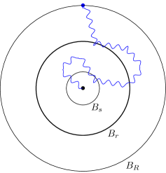
Figure 2. An instance of a rotor walk $(X_{t}^{(R)},\rho_{t}^{(R)})_{t\geq 0}$ terminated upon visiting the boundary $Z_{R}$ of the ball $B_{R}$, where the trajectory of the walker is given by the (blue) squiggly path. Here the last visit to the ball $B_{s}$ is before the first visit to the boundary $Z_{r}$ of the ball $B_{r}$, and therefore terminating this walk prematurely upon visiting $Z_{r}$ (instead of $Z_{R}$) will not change the rotor of vertices in $B_{s}$ in the final rotor configuration.

Condition (S2) is useful for deriving other results provided that we already know that $\operatorname{\mathchoice{\vbox{\halign{#\cr\arrowfill@\relbar\relbar\rightharpoonup{\scriptstyle}\crcr\nointerlineskip\cr$\hfil\displaystyle\mathsf{WUSF}\hfil$\crcr}}}{\vbox{\halign{#\cr\arrowfill@\relbar\relbar\rightharpoonup{\scriptstyle}\crcr\nointerlineskip\cr$\hfil\textstyle\mathsf{WUSF}\hfil$\crcr}}}{\vbox{\halign{#\cr\arrowfill@\relbar\relbar\rightharpoonup{\scriptscriptstyle}\crcr\nointerlineskip\cr$\hfil\scriptstyle\mathsf{WUSF}\hfil$\crcr}}}{\vbox{\halign{#\cr\arrowfill@\relbar\relbar\rightharpoonup{\scriptscriptstyle}\crcr\nointerlineskip\cr$\hfil\scriptscriptstyle\mathsf{WUSF}\hfil$\crcr}}}}(G)$ is rotor walk stationary; Theorem 1.5 will be proved in this way. Condition (S3) is useful for checking rotor walk stationarity as it reduces the problem to rotor walks on finite graphs, which is more well-studied in the literature; Proposition 7.1 in Section 7 will be proved in this way.

We now provide a sketch of how (S2) and (S3) imply the rotor walk stationarity of $\operatorname{\mathchoice{\vbox{\halign{#\cr\arrowfill@\relbar\relbar\rightharpoonup{\scriptstyle}\crcr\nointerlineskip\cr$\hfil\displaystyle\mathsf{WUSF}\hfil$\crcr}}}{\vbox{\halign{#\cr\arrowfill@\relbar\relbar\rightharpoonup{\scriptstyle}\crcr\nointerlineskip\cr$\hfil\textstyle\mathsf{WUSF}\hfil$\crcr}}}{\vbox{\halign{#\cr\arrowfill@\relbar\relbar\rightharpoonup{\scriptscriptstyle}\crcr\nointerlineskip\cr$\hfil\scriptstyle\mathsf{WUSF}\hfil$\crcr}}}{\vbox{\halign{#\cr\arrowfill@\relbar\relbar\rightharpoonup{\scriptscriptstyle}\crcr\nointerlineskip\cr$\hfil\scriptscriptstyle\mathsf{WUSF}\hfil$\crcr}}}}(G)$. The idea is to relate the rotor walk on $G$ to the rotor walk on its exhaustion $(G_{R})_{R\geq 0}$. We first approximate the rotor walks on those graphs uniformly by the rotor walks that is terminated upon visiting the boundary of the ball $B_{r}$ for a fixed radius $r>0$ that is sufficiently large. The latter walk in turn depends only on rotors of (finitely many) vertices in $B_{r}$. It then follows from (7) that the rotor walk on $G$ with sink $Z_{r}=\partial B_{r}$ can be taken as the limit of the rotor walk on $G_{R}$ with the same sink $Z_{r}$ as $R\to\infty$. The stationarity of the wired uniform spanning forest for the rotor walk on $G$ then follows as the consequence of the stationarity of the uniform spannning forest for rotor walks on the finite graphs $(G_{R})_{R\geq 0}$ (Proposition 7.1).

The crucial step here is to find the radius $r>0$ such that the rotor walks on $G_{R}$ with sink $Z_{R}$ can be uniformly approximated by the (shorter) rotor walks with sink $Z_{r}$. Indeed, we will see that condition (S2) and (S3) are essentially equivalent to requiring that such a radius exists. Note that such a radius does not always exist, as can be seen from the following example.

Example 6.3.

Let $G$ be the $2$-ary tree $\operatorname{\mathbb{T}}_{2}$ with an infinite path attached to its root from Figure 1. That is,

$$V(G):= V(\operatorname{\mathbb{T}}_{2})\cup\{y_{i}\mid i\geq 0\};$$

$$E(G):= E(\operatorname{\mathbb{T}}_{2})\cup\{\{o,y_{0}\}\}\cup\{\{y_{i},y_{i+1}\}\mid i\geq 0\},$$

where $o$ is the root of $\operatorname{\mathbb{T}}_{2}$.

We will perform two rotor walks on $G_{R}$ $(R\geq 0)$. Both walks have the same initial location $y_{0}$ and the same initial rotor configuration $\rho_{R}$ sampled from $\operatorname{\mathchoice{\vbox{\halign{#\cr\arrowfill@\relbar\relbar\rightharpoonup{\scriptstyle}\crcr\nointerlineskip\cr$\hfil\displaystyle\mathsf{USF}\hfil$\crcr}}}{\vbox{\halign{#\cr\arrowfill@\relbar\relbar\rightharpoonup{\scriptstyle}\crcr\nointerlineskip\cr$\hfil\textstyle\mathsf{USF}\hfil$\crcr}}}{\vbox{\halign{#\cr\arrowfill@\relbar\relbar\rightharpoonup{\scriptscriptstyle}\crcr\nointerlineskip\cr$\hfil\scriptstyle\mathsf{USF}\hfil$\crcr}}}{\vbox{\halign{#\cr\arrowfill@\relbar\relbar\rightharpoonup{\scriptscriptstyle}\crcr\nointerlineskip\cr$\hfil\scriptscriptstyle\mathsf{USF}\hfil$\crcr}}}}(G_{R},Z_{R})$, but with two different choices for the sink; see Figure 3.

(a)

(b)

(c)

Figure 3. (a) An initial rotor configuration sampled from $\operatorname{\mathchoice{\vbox{\halign{#\cr\arrowfill@\relbar\relbar\rightharpoonup{\scriptstyle}\crcr\nointerlineskip\cr$\hfil\displaystyle\mathsf{USF}\hfil$\crcr}}}{\vbox{\halign{#\cr\arrowfill@\relbar\relbar\rightharpoonup{\scriptstyle}\crcr\nointerlineskip\cr$\hfil\textstyle\mathsf{USF}\hfil$\crcr}}}{\vbox{\halign{#\cr\arrowfill@\relbar\relbar\rightharpoonup{\scriptscriptstyle}\crcr\nointerlineskip\cr$\hfil\scriptstyle\mathsf{USF}\hfil$\crcr}}}{\vbox{\halign{#\cr\arrowfill@\relbar\relbar\rightharpoonup{\scriptscriptstyle}\crcr\nointerlineskip\cr$\hfil\scriptscriptstyle\mathsf{USF}\hfil$\crcr}}}}(G_{R},Z_{R})$ with a walker initially located at $y_{0}$. (b)First, the walker walks toward $y_{R}$ until it is stopped at $y_{r}\in Z_{r}$. (c) Then, the walker resumes walking toward $y_{R}$ until it reaches $y_{k}$. (d) Finally, the walker walks toward the root until it reaches the root.

First, consider the rotor walk on $G_{R}$ terminated upon visiting $Z_{r}$, where $r$ is a fixed integer. As $\rho_{R}$ is sampled from $\operatorname{\mathchoice{\vbox{\halign{#\cr\arrowfill@\relbar\relbar\rightharpoonup{\scriptstyle}\crcr\nointerlineskip\cr$\hfil\displaystyle\mathsf{USF}\hfil$\crcr}}}{\vbox{\halign{#\cr\arrowfill@\relbar\relbar\rightharpoonup{\scriptstyle}\crcr\nointerlineskip\cr$\hfil\textstyle\mathsf{USF}\hfil$\crcr}}}{\vbox{\halign{#\cr\arrowfill@\relbar\relbar\rightharpoonup{\scriptscriptstyle}\crcr\nointerlineskip\cr$\hfil\scriptstyle\mathsf{USF}\hfil$\crcr}}}{\vbox{\halign{#\cr\arrowfill@\relbar\relbar\rightharpoonup{\scriptscriptstyle}\crcr\nointerlineskip\cr$\hfil\scriptscriptstyle\mathsf{USF}\hfil$\crcr}}}}(G_{R},Z_{R})$, we have with probability approximately $1-\epsilon$ $(\epsilon>0$) that

$$\rho(y_{i+1})=y_{i}\qquad\forall\ i\leq\epsilon R.$$

It then follows that the walker will walk toward $y_{{R}}$ for the first $\epsilon R$ steps of the rotor walk; see Figure 3(b). Since $r\leq\epsilon R$ for sufficiently large $R$, this rotor walk will terminate in less than $\epsilon R$ steps as it has visited $y_{r}\in Z_{r}$ by then. In particular, this implies that, with probability close to $1$, we have

$$u_{G_{R},Z_{r}}(\rho_{R},y_{0})=1,$$ (13)

as this walk visits $y_{0}$ exactly once (namely at the $0$-th step of the walk).

Now, consider the rotor walk on $G_{R}$ terminated upon visiting $Z_{R}$. As $\rho_{R}$ is sampled from $\operatorname{\mathchoice{\vbox{\halign{#\cr\arrowfill@\relbar\relbar\rightharpoonup{\scriptstyle}\crcr\nointerlineskip\cr$\hfil\displaystyle\mathsf{USF}\hfil$\crcr}}}{\vbox{\halign{#\cr\arrowfill@\relbar\relbar\rightharpoonup{\scriptstyle}\crcr\nointerlineskip\cr$\hfil\textstyle\mathsf{USF}\hfil$\crcr}}}{\vbox{\halign{#\cr\arrowfill@\relbar\relbar\rightharpoonup{\scriptscriptstyle}\crcr\nointerlineskip\cr$\hfil\scriptstyle\mathsf{USF}\hfil$\crcr}}}{\vbox{\halign{#\cr\arrowfill@\relbar\relbar\rightharpoonup{\scriptscriptstyle}\crcr\nointerlineskip\cr$\hfil\scriptscriptstyle\mathsf{USF}\hfil$\crcr}}}}(G_{R},Z_{R})$, we have with probability approximately $1-\frac{1}{R}$ that

$$\exists\ i\leq R\quad\text{s.t.}\quad\rho(y_{i})=y_{i+1}.$$

Let $k$ be the smallest positive integer satisfying this property. It then follows that the walker will walk toward $y_{R}$ for the first $k$ steps of the walk, then turn to walk toward the root for the next $k+1$ steps; see Figure 3(c) and 3(d). Also note that this rotor walk will not terminate before the first $2k+1$ steps as it has not visited $Z_{R}$ yet. In particular, this implies that, with probability close to 1, we have

$$u_{G_{R},Z_{R}}(\rho_{R},y_{0})\geq 2,$$ (14)

as this walk has visited $y_{0}$ at least twice (namely at the $0$-th and $2k$-th step of the walk).

Hence we conclude from (13) and (14) that the rotor walks on $G_{R}$ with sink $Z_{R}$ cannot be uniformly approximated by the rotor walks with sink $Z_{r}$ for any fixed $r\geq 0$. ∎

We now build present the proof of the first part of Theorem 6.2. Recall the definition of occupation rate ${S_{n}}/{n}$ from Definition 2.4.

Proof of (S1) implies (S2).

Since $\operatorname{\mathchoice{\vbox{\halign{#\cr\arrowfill@\relbar\relbar\rightharpoonup{\scriptstyle}\crcr\nointerlineskip\cr$\hfil\displaystyle\mathsf{WUSF}\hfil$\crcr}}}{\vbox{\halign{#\cr\arrowfill@\relbar\relbar\rightharpoonup{\scriptstyle}\crcr\nointerlineskip\cr$\hfil\textstyle\mathsf{WUSF}\hfil$\crcr}}}{\vbox{\halign{#\cr\arrowfill@\relbar\relbar\rightharpoonup{\scriptscriptstyle}\crcr\nointerlineskip\cr$\hfil\scriptstyle\mathsf{WUSF}\hfil$\crcr}}}{\vbox{\halign{#\cr\arrowfill@\relbar\relbar\rightharpoonup{\scriptscriptstyle}\crcr\nointerlineskip\cr$\hfil\scriptscriptstyle\mathsf{WUSF}\hfil$\crcr}}}}(G)$ is rotor walk stationary, we have:

$$\operatorname{\mathbb{E}}_{\rho}[{u(\rho,x)}]=\sum_{i=0}^{n-1}\operatorname{\mathbb{E}}_{\rho}\left[\frac{u(\sigma^{i}(\rho),x)}{n}\right]=\operatorname{\mathbb{E}}_{\rho}\left[\frac{S_{n}(\rho,x)}{n}\right].$$

We also have by Lemma 5.1 that

$$\liminf_{n\to\infty}\frac{S_{n}(\rho,x)}{n}\geq\operatorname{\mathcal{G}}(x),$$

for any rotor configuration $\rho$. These two observations give us:

$$\operatorname{\mathbb{E}}_{\rho}[{u(\rho,x)}]=\liminf_{n\to\infty}\operatorname{\mathbb{E}}_{\rho}\left[\frac{S_{n}(\rho,x)}{n}\right]\geq\operatorname{\mathbb{E}}_{\rho}\left[\liminf_{n\to\infty}\frac{S_{n}(\rho,x)}{n}\right]\geq\operatorname{\mathcal{G}}(x),$$

where the first inequality is due to Fatou’s lemma. Finally, we have from Theorem 1.1 that

$$\operatorname{\mathbb{E}}_{\rho}[{u(\rho,x)}]\leq\operatorname{\mathcal{G}}(x).$$

Hence we conclude that $\operatorname{\mathbb{E}}_{\rho}[u(\rho,x)]=\operatorname{\mathcal{G}}(x)$, as desired. ∎

We now present the proof of the second part of Theorem 6.2.

Proof of (S2) implies (S3).

Let $u(R,r):=u_{G_{R},Z_{r}}(\rho_{R},B_{s})$ be the number of visits to the ball $B_{s}$ by the rotor walk $(X_{t}^{(R)})_{t\geq 0}$ that is terminated strictly before hitting $Z_{r}$. Note that the set of vertices visited before the last visit to $B_{s}$ is contained in the ball $B_{r}$ if and only if the walker never comes back to visit $B_{s}$ after hitting the boundary $Z_{r}=\partial B_{r}$ of the ball $B_{r}$ (see Figure 2). This happens if and only if the number of visits to $B_{s}$ by the rotor walk terminated upon hitting $Z_{r}$ is equal to the same number if the rotor walk is not terminated prematurely. That is to say, for $r\leq R$,

$$\operatorname{\mathbb{P}}[\{X_{t}^{(R)}\mid t\leq t_{R}(s)\}\subseteq B_{r}]=\operatorname{\mathbb{E}}_{\rho_{R}}\left[\mathbbm{1}\left\{u(R,R)-u(R,r)=0\right\}\right].$$

Now note that

$$\begin{split}\operatorname{\mathbb{E}}_{\rho_{R}}\left[\mathbbm{1}\left\{u(R,R)-u(R,r)=0\right\}\right]\geq 1-\operatorname{\mathbb{E}}_{\rho_{R}}[u(R,R)]-\operatorname{\mathbb{E}}_{\rho_{R}}[u(R,r)].\end{split}$$

It then suffices to show that $\lim_{R\to\infty}\operatorname{\mathbb{E}}_{\rho_{R}}[u(R,R)]-\operatorname{\mathbb{E}}_{\rho_{R}}[u(R,r)]\leq\epsilon$.

Now note that, we have by the stationarity of $\operatorname{\mathchoice{\vbox{\halign{#\cr\arrowfill@\relbar\relbar\rightharpoonup{\scriptstyle}\crcr\nointerlineskip\cr$\hfil\displaystyle\mathsf{USF}\hfil$\crcr}}}{\vbox{\halign{#\cr\arrowfill@\relbar\relbar\rightharpoonup{\scriptstyle}\crcr\nointerlineskip\cr$\hfil\textstyle\mathsf{USF}\hfil$\crcr}}}{\vbox{\halign{#\cr\arrowfill@\relbar\relbar\rightharpoonup{\scriptscriptstyle}\crcr\nointerlineskip\cr$\hfil\scriptstyle\mathsf{USF}\hfil$\crcr}}}{\vbox{\halign{#\cr\arrowfill@\relbar\relbar\rightharpoonup{\scriptscriptstyle}\crcr\nointerlineskip\cr$\hfil\scriptscriptstyle\mathsf{USF}\hfil$\crcr}}}}(G_{R},Z_{R})$ for rotor walks on finite graphs (Proposition 3.4) that:

$$\operatorname{\mathbb{E}}_{\rho_{R}}[u(R,R)]=\operatorname{\mathbb{E}}_{\rho_{R}}[u_{G_{R},Z_{R}}(\rho_{R},B_{s})]=\operatorname{\mathcal{G}}_{G_{R},Z_{R}}(B_{s}).$$

By taking the limit as $R\to\infty$, we get

$$\lim_{R\to\infty}\operatorname{\mathbb{E}}_{\rho_{R}}[u(R,R)]=\operatorname{\mathcal{G}}_{G,\varnothing}(B_{s}).$$ (15)

On the other hand, the number of visits to $B_{s}$ strictly before the walker hits $Z_{r}$ is an event that only depends on the rotors in the ball $B_{r}$ (of which there are only finitely many of them). Hence we have by (7) that

$$\lim_{R\to\infty}\operatorname{\mathbb{E}}_{\rho_{R}}[u(R,r)]=\lim_{R\to\infty}\operatorname{\mathbb{E}}_{\rho_{R}}[u_{G_{R},Z_{r}}(\rho_{R},B_{s})]=\operatorname{\mathbb{E}}_{\rho}[u_{G,Z_{r}}(\rho,B_{s})].$$

Now note that $u_{G,Z_{r}}$ increases to $u_{G,\varnothing}$ as $r\to\infty$. By the monotone convergence theorem, we then have for sufficiently large $r$ that

$$\operatorname{\mathbb{E}}_{\rho}[u_{G,Z_{r}}(\rho,B_{s})]\geq\operatorname{\mathbb{E}}_{\rho}[u_{G,\varnothing}(\rho,B_{s})]-\epsilon.$$

Together with condition (S2) that $\operatorname{\mathbb{E}}_{\rho}[u_{G,\varnothing}(\rho,B_{s})]=\operatorname{\mathcal{G}}_{G,\varnothing}(B_{s})$, the two observations above imply that

$$\lim_{R\to\infty}\operatorname{\mathbb{E}}_{\rho_{R}}[u(R,r)]\geq\operatorname{\mathcal{G}}_{G,\varnothing}(B_{s})-\epsilon.$$ (16)

Subtracting (16) from (15), we get

$$\lim_{R\to\infty}\operatorname{\mathbb{E}}_{\rho_{R}}[u(R,R)]-\operatorname{\mathbb{E}}_{\rho_{R}}[u(R,r)]\leq\epsilon,$$

as desired. ∎

We now present the proof of the last part of Theorem 6.2.

Proof of (S3) implies (S1).

It suffices to show that $\operatorname{\mathbb{P}}_{\rho}[B\subseteq\sigma_{G}(\rho)]=\operatorname{\mathbb{P}}_{\rho}[B\subseteq\rho]$ for any finite set $B$ of directed edges of $G$.

Let $\epsilon>0$ be any positive real number. Let $s$ be the smallest integer such that all vertices incident to $B$ are contained in $B_{s}$. Consider the rotor walk on $G$ with initial rotor configuration $\rho$ and with empty sink. Since this walk is transient almost surely (by Corollary 4.3), the probability that the walker returns to visit $B_{s}$ again after hitting $Z_{r}=\partial B(a,r)$ converges to $0$ as $r\to\infty$. Also note that the rotors in the ball $B_{s}$ will stay constant if the walker never returns to visit $B_{s}$ again. Hence, for sufficiently large $r\geq s$, we have:

$$\left|\operatorname{\mathbb{P}}_{\rho}[B\subseteq\sigma_{G}(\rho)]-\operatorname{\mathbb{P}}_{\rho}[B\subseteq\sigma_{G,Z_{r}}(\rho)]\right|\leq\frac{\epsilon}{2}.$$

Now note that the rotors of $\sigma_{G,Z_{r}}(\rho)$ in $B_{s}$ depends only at the rotors of $\rho$ in the ball $B_{r}$ as the walk is terminated upon hitting $Z_{r}$. Since this is a finite set, we have by (7) that

$$\operatorname{\mathbb{P}}_{\rho}[B\subseteq\sigma_{G,Z_{r}}(\rho)]=\lim_{R\to\infty}\operatorname{\mathbb{P}}_{\rho_{R}}[B\subseteq\sigma_{G_{R},Z_{r}}(\rho_{R})].$$

It then suffices to show that

$$\left|\lim_{R\to\infty}\operatorname{\mathbb{P}}_{\rho_{R}}[B\subseteq\sigma_{G_{R},Z_{r}}(\rho_{R})]-\operatorname{\mathbb{P}}_{\rho}[B\subseteq\rho]\right|\leq\frac{\epsilon}{2}.$$

Now consider the rotor walk on $G_{R}$ with initial rotor configuration $\rho_{R}$ that is terminated upon hitting $Z_{R}$. Suppose that the walk never returns to visit $B_{s}$ again after it hits $Z_{r}$. Then the rotors in the ball $B_{s}$ of the final rotor configuration remains unchanged even if the walk is terminated prematurely upon visiting $Z_{r}$ (see Figure 2). Since $B$ is contained in $B_{s}$, this means that $B$ is contained in $\sigma_{G_{R},Z_{r}}(\rho_{R})$ if and only if $B$ is contained in $\sigma_{G_{R},Z_{R}}(\rho_{R})$. Hence we have:

$$\{X_{t}^{(R)}\mid t\leq t_{R}(s)\}\subseteq B_{r}\quad\Rightarrow\quad\mathbbm{1}\{B\subseteq\sigma_{G_{R},Z_{r}}(\rho_{R})\}=\mathbbm{1}\{B\subseteq\sigma_{G_{R},Z_{R}}(\rho_{R})\}.$$

Now note that by (S3) the event $\{X_{t}^{(R)}\mid t\leq t_{R}(s)\}$ occurs with probability at least $1-\frac{\epsilon}{2}$ for sufficiently large $r$. It then follows that, for sufficiently large $r$,

$$\left|\operatorname{\mathbb{P}}_{\rho_{R}}[B\subseteq\sigma_{G_{R},Z_{r}}(\rho_{R})]-\operatorname{\mathbb{P}}_{\rho_{R}}[B\subseteq\sigma_{G_{R},Z_{R}}(\rho_{R})]\right|\leq\frac{\epsilon}{2}.$$

On the other hand, the rotor configuration $\sigma_{G_{R},Z_{R}}(\rho_{R})$ has the same law as $\rho_{R}$ by the stationarity of $\operatorname{\mathchoice{\vbox{\halign{#\cr\arrowfill@\relbar\relbar\rightharpoonup{\scriptstyle}\crcr\nointerlineskip\cr$\hfil\displaystyle\mathsf{USF}\hfil$\crcr}}}{\vbox{\halign{#\cr\arrowfill@\relbar\relbar\rightharpoonup{\scriptstyle}\crcr\nointerlineskip\cr$\hfil\textstyle\mathsf{USF}\hfil$\crcr}}}{\vbox{\halign{#\cr\arrowfill@\relbar\relbar\rightharpoonup{\scriptscriptstyle}\crcr\nointerlineskip\cr$\hfil\scriptstyle\mathsf{USF}\hfil$\crcr}}}{\vbox{\halign{#\cr\arrowfill@\relbar\relbar\rightharpoonup{\scriptscriptstyle}\crcr\nointerlineskip\cr$\hfil\scriptscriptstyle\mathsf{USF}\hfil$\crcr}}}}(G_{R},Z_{R})$ for rotor walks on finite graphs (Proposition 3.3). These two facts then imply that:

$$\left|\operatorname{\mathbb{P}}_{\rho_{R}}[B\subseteq\sigma_{G_{R},Z_{r}}(\rho_{R})]-\operatorname{\mathbb{P}}_{\rho_{R}}[B\subseteq\rho_{R}]\right|\leq\frac{\epsilon}{2}.$$

Taking the limit of the inequality above as $R\to\infty$ and then applying (7) to $\lim_{R\to\infty}\operatorname{\mathbb{P}}_{\rho_{R}}[B\subseteq\rho_{R}]$, we then conclude that

$$\left|\lim_{R\to\infty}\operatorname{\mathbb{P}}_{\rho_{R}}[B\subseteq\sigma_{G_{R},Z_{r}}(\rho_{R})]-\operatorname{\mathbb{P}}_{\rho}[B\subseteq\rho]\right|\leq\frac{\epsilon}{2}.$$

This completes the proof. ∎

7. A sufficient condition for rotor walk stationarity

In this section we show that the oriented wired spanning forest is always rotor walk stationary for a family of trees that includes the $b$-ary tree $\operatorname{\mathbb{T}}_{b}$ ($b\geq 2$). We will need the following notations to describe this family of trees.

Let $\rho$ be a rotor configuration that is an oriented spanning forest of $G$ (recall that we consider $\rho$ both as a rotor configuration and an oriented subgraph of $G$). An backward path (resp. forward path) in $\rho$ is a sequence $\langle x_{0},x_{1},x_{2},\ldots\rangle$ such that $\rho(x_{i+1})=x_{i}$ (resp. $\rho(x_{i})=x_{i+1}$) for every $i\geq 0$. A path is infinite if it contains infinitely many vertices.

Since $\rho$ is an oriented spanning forest, for each vertex $a$ the subgraph $\rho$ has a unique oriented tree that contains $a$, and this oriented tree has a unique maximal forward path that starts at $a$. We denote by $T(a,\rho)$ this unique tree, and by $P(a,\rho)$ this unique maximal forward path.

A vertex $x$ of $G$ is complete in $\rho$ if $T(x,\rho)$ contains all neighbors of $x$ in $G$; and is incomplete otherwise.

Proposition 7.1.

Let $G$ be a tree that is locally finite and transient, and let $a$ be a vertex of $G$. Consider any rotor walk on $G$ with initial location $a$ and with empty sink. Suppose that the rotor configuration $\rho$ sampled from $\operatorname{\mathchoice{\vbox{\halign{#\cr\arrowfill@\relbar\relbar\rightharpoonup{\scriptstyle}\crcr\nointerlineskip\cr$\hfil\displaystyle\mathsf{WUSF}\hfil$\crcr}}}{\vbox{\halign{#\cr\arrowfill@\relbar\relbar\rightharpoonup{\scriptstyle}\crcr\nointerlineskip\cr$\hfil\textstyle\mathsf{WUSF}\hfil$\crcr}}}{\vbox{\halign{#\cr\arrowfill@\relbar\relbar\rightharpoonup{\scriptscriptstyle}\crcr\nointerlineskip\cr$\hfil\scriptstyle\mathsf{WUSF}\hfil$\crcr}}}{\vbox{\halign{#\cr\arrowfill@\relbar\relbar\rightharpoonup{\scriptscriptstyle}\crcr\nointerlineskip\cr$\hfil\scriptscriptstyle\mathsf{WUSF}\hfil$\crcr}}}}(G)$ satisfies these two conditions almost surely:

1. $T(a,\rho)$ has no infinite backward path; and

2. There are infinitely many incomplete vertices in $P(a,\rho)$.

Then $\operatorname{\mathchoice{\vbox{\halign{#\cr\arrowfill@\relbar\relbar\rightharpoonup{\scriptstyle}\crcr\nointerlineskip\cr$\hfil\displaystyle\mathsf{WUSF}\hfil$\crcr}}}{\vbox{\halign{#\cr\arrowfill@\relbar\relbar\rightharpoonup{\scriptstyle}\crcr\nointerlineskip\cr$\hfil\textstyle\mathsf{WUSF}\hfil$\crcr}}}{\vbox{\halign{#\cr\arrowfill@\relbar\relbar\rightharpoonup{\scriptscriptstyle}\crcr\nointerlineskip\cr$\hfil\scriptstyle\mathsf{WUSF}\hfil$\crcr}}}{\vbox{\halign{#\cr\arrowfill@\relbar\relbar\rightharpoonup{\scriptscriptstyle}\crcr\nointerlineskip\cr$\hfil\scriptscriptstyle\mathsf{WUSF}\hfil$\crcr}}}}(G)$ is rotor walk stationary.

In order to show that the $b$-ary tree $\operatorname{\mathbb{T}}_{b}$ $(b\geq 2)$ satisfies the two conditions in Proposition 7.1, we need the following two properties of the oriented subgraph $\rho$ sampled from $\operatorname{\mathchoice{\vbox{\halign{#\cr\arrowfill@\relbar\relbar\rightharpoonup{\scriptstyle}\crcr\nointerlineskip\cr$\hfil\displaystyle\mathsf{WUSF}\hfil$\crcr}}}{\vbox{\halign{#\cr\arrowfill@\relbar\relbar\rightharpoonup{\scriptstyle}\crcr\nointerlineskip\cr$\hfil\textstyle\mathsf{WUSF}\hfil$\crcr}}}{\vbox{\halign{#\cr\arrowfill@\relbar\relbar\rightharpoonup{\scriptscriptstyle}\crcr\nointerlineskip\cr$\hfil\scriptstyle\mathsf{WUSF}\hfil$\crcr}}}{\vbox{\halign{#\cr\arrowfill@\relbar\relbar\rightharpoonup{\scriptscriptstyle}\crcr\nointerlineskip\cr$\hfil\scriptscriptstyle\mathsf{WUSF}\hfil$\crcr}}}}(\operatorname{\mathbb{T}}_{b})$:

1. The underlying graph $H$ of any oriented trees of $\rho$ has exactly one end (i.e. any two infinite unoriented paths in $H$ can differ by at most finitely many vertices) almost surely.

2. Let $\langle x_{0},x_{1},x_{2},\ldots\rangle$ be the path $P(a,\rho)$, and let $E_{i}$ $(i\geq 1)$ be the event that $x_{i}$ is incomplete in $\rho$. Then $(E_{i})_{i\geq 1}$ are independent events, and each event has probability $\operatorname{\mathbb{P}}(E_{i})=1-\left(1/b\right)^{b-1}$ to occur.

Indeed, these two properties can be deduced from Wilson’s method oriented toward infinity, and we refer to [LP16, Section 10.6] for proofs. Now note that conditition (i) in Proposition 7.1 follows from (a), and conditition (ii) follows from (b).

We now build toward the proof of Proposition 7.1. Our proof relies on the following crucial yet simple observation: If a vertex $x$ was visited during the walk, then $x$ is contained in the same weak component of the final rotor configuration as the initial location $a$.

Consider a transient rotor walk $(X_{t})_{t\geq 0}$ on $G$. For any vertex $x$ of $G$ that was visited by the rotor walk, we denote by $\operatorname{\textnormal{FV}}(x):=\operatorname{\textnormal{FV}}_{G,Z}(\rho,x)$ and $\operatorname{\textnormal{LV}}(x):=\operatorname{\textnormal{LV}}_{G,Z}(\rho,x)$ the first time and the last time the vertex $x$ being visited by the rotor walk, respectively, i.e.

$$\begin{split}\operatorname{\textnormal{FV}}(x)&:=\min\{t\geq 0\mid X_{t}=x\};\\ \operatorname{\textnormal{LV}}(x)&:=\max\{t\geq 0\mid X_{t}=x\}.\end{split}$$

Lemma 7.2.

Let $G$ be a tree that is locally finite. Consider any rotor walk on $G$ with initial location $a$, initial rotor configuration $\rho$, and (not necessarily empty) sink $Z$. Suppose that this rotor walk is transient, and let $\xi:=\sigma(\rho)$ be the final rotor configuration of this walk. Then, for any vertex $x_{i}$ in $P(a,\xi):=\langle x_{0},x_{1},x_{2},\ldots\rangle$ that is incomplete in $\xi$, we have

$$\operatorname{\textnormal{FV}}(x_{i+1})=\operatorname{\textnormal{LV}}(x_{i})+1.$$

That is, the first visit of $x_{i+1}$ was right after the last visit of $x_{i}$.

Proof.

Since $\xi(x_{i})=x_{i+1}$, it follows that the walker moved toward $x_{i}$ right after the last visit to $x_{i}$ (i.e. $X_{t}=x_{i+1}$ with $t=\operatorname{\textnormal{LV}}(x_{i})+1$). It then suffices to show that $t_{1}:=\operatorname{\textnormal{LV}}(x_{i})+1$ is the first visit to $x_{i+1}$.

Suppose to the contrary that $t_{2}:=\operatorname{\textnormal{FV}}(x_{i+1})$ is strictly smaller than $t_{1}$. Now note that $X_{t_{2}-1}=x_{i}$ since the unique path from $a$ to $x_{i+1}$ in $G$ goes through $x_{i}$ (as $G$ is a tree). Since $X_{t_{2}-1}=X_{t_{1}-1}=x_{i}$ and $t_{2}<t_{1}$, it follows from the mechanism of the rotor walk that every neighbor of $x_{i}$ in $G$ was visited by the walker in between the $t_{2}-1$-th and $t_{1}-1$-th step of the walk. This implies that every neighbor of $x_{i}$ is contained in the same component as $x_{i}$ in the final rotor configuration $\xi$, and hence $x_{i}$ is a complete vertex in $\xi$. This contradicts our assumption that $x_{i}$ is incomplete in $\xi$, as desired. ∎

For any vertex $x$ of $G$, we denote by $W(\rho,x)$ the set of vertices of $G$ with a directed path in $\rho$ from the vertex to $x$, i.e.

$$W(\rho,x):=\{y\mid\exists\,\langle y=x_{0},\ldots,x_{n}=x\rangle\text{ s.t. }\rho(x_{i})=x_{i+1}\ \forall\ i<n\}.$$

Lemma 7.3.

Let $G$ be a tree that is locally finite. Consider any rotor walk $(X_{t},\rho_{t})_{t\geq 0}$ on $G$ with initial location $a$, initial rotor configuration $\rho$, and (not necessarily empty) sink Z. Suppose that the rotor walk is transient, and let $\xi:=\sigma(\rho)$ be the final rotor configuration of this walk. Then, for any vertex $x$ in $P(a,\xi)$ that is incomplete in $\xi$, we have

$$\{X_{t}\mid t\leq\operatorname{\textnormal{LV}}(x)\}\subseteq W(\xi,x).$$

Proof.

Let $P(a,\xi):=\langle x_{0},x_{1},x_{2},\ldots\rangle$, and let $x=x_{i}$ be an incomplete vertex in $\xi$. By Lemma 7.2, the walker had not visited $x_{i+1}$ yet during the first $\operatorname{\textnormal{LV}}(x_{i})$-th step of the walk. Since $G$ is a tree, this means that, during the first $\operatorname{\textnormal{LV}}(x_{i})$-th step of the walk, the walker has only visited vertices in the weak component of $G\setminus\{x_{i},x_{i+1}\}$ that contains $x_{i}$. On the other hand, all vertices visited by the walker are in the weak component of $a$ in $\xi$. Now note that the intersection of these two components is equal to $W(\xi,x_{i})$, and the lemma now follows. ∎

We now present the proof of Proposition 7.1.

Proof of Proposition 7.1.

It suffices to check that condition (S3) in Theorem 6.2 is satisfied. That is, for any $\epsilon>0$ and any $s>0$, we have for sufficiently large $r$ that

$$\lim_{R\to\infty}\operatorname{\mathbb{P}}[\{X_{t}^{(R)}\mid t\leq t_{R}(s)\}\subseteq B_{r}]\geq 1-\epsilon,$$

where $(X_{t}^{(R)},\rho_{t}^{(R)})$ is the rotor walk on $G_{R}$ with initial location $a$, with initial rotor configuration $\rho_{R}$ sampled from $\operatorname{\mathchoice{\vbox{\halign{#\cr\arrowfill@\relbar\relbar\rightharpoonup{\scriptstyle}\crcr\nointerlineskip\cr$\hfil\displaystyle\mathsf{USF}\hfil$\crcr}}}{\vbox{\halign{#\cr\arrowfill@\relbar\relbar\rightharpoonup{\scriptstyle}\crcr\nointerlineskip\cr$\hfil\textstyle\mathsf{USF}\hfil$\crcr}}}{\vbox{\halign{#\cr\arrowfill@\relbar\relbar\rightharpoonup{\scriptscriptstyle}\crcr\nointerlineskip\cr$\hfil\scriptstyle\mathsf{USF}\hfil$\crcr}}}{\vbox{\halign{#\cr\arrowfill@\relbar\relbar\rightharpoonup{\scriptscriptstyle}\crcr\nointerlineskip\cr$\hfil\scriptscriptstyle\mathsf{USF}\hfil$\crcr}}}}(G_{R},Z_{R})$, and with sink $Z_{R}$. The integer $t_{R}(s)$ is the last visit of $B_{s}$.

Let $\xi_{R}:=\sigma_{G_{R},Z_{R}}(\rho_{R})$ be the final rotor configuration of the rotor walk $(X_{t}^{(R)},\rho_{t}^{(R)})$. Note that $\xi_{R}\overset{d}{=}\operatorname{\mathchoice{\vbox{\halign{#\cr\arrowfill@\relbar\relbar\rightharpoonup{\scriptstyle}\crcr\nointerlineskip\cr$\hfil\displaystyle\mathsf{USF}\hfil$\crcr}}}{\vbox{\halign{#\cr\arrowfill@\relbar\relbar\rightharpoonup{\scriptstyle}\crcr\nointerlineskip\cr$\hfil\textstyle\mathsf{USF}\hfil$\crcr}}}{\vbox{\halign{#\cr\arrowfill@\relbar\relbar\rightharpoonup{\scriptscriptstyle}\crcr\nointerlineskip\cr$\hfil\scriptstyle\mathsf{USF}\hfil$\crcr}}}{\vbox{\halign{#\cr\arrowfill@\relbar\relbar\rightharpoonup{\scriptscriptstyle}\crcr\nointerlineskip\cr$\hfil\scriptscriptstyle\mathsf{USF}\hfil$\crcr}}}}(G_{R},Z_{R})$ by the rotor walk stationarity of $\operatorname{\mathchoice{\vbox{\halign{#\cr\arrowfill@\relbar\relbar\rightharpoonup{\scriptstyle}\crcr\nointerlineskip\cr$\hfil\displaystyle\mathsf{USF}\hfil$\crcr}}}{\vbox{\halign{#\cr\arrowfill@\relbar\relbar\rightharpoonup{\scriptstyle}\crcr\nointerlineskip\cr$\hfil\textstyle\mathsf{USF}\hfil$\crcr}}}{\vbox{\halign{#\cr\arrowfill@\relbar\relbar\rightharpoonup{\scriptscriptstyle}\crcr\nointerlineskip\cr$\hfil\scriptstyle\mathsf{USF}\hfil$\crcr}}}{\vbox{\halign{#\cr\arrowfill@\relbar\relbar\rightharpoonup{\scriptscriptstyle}\crcr\nointerlineskip\cr$\hfil\scriptscriptstyle\mathsf{USF}\hfil$\crcr}}}}(G_{R},Z_{R})$ for finite graphs (Proposition 3.3).

Fix $r\geq 0$. For any rotor configuration $\rho$, let $E_{r}(\rho)$ be the event that that there exists a vertex $x$ such that

1. $x$ is an incomplete vertex in $\rho$ that is contained in $P(a,\rho)\cap(B_{r}\setminus B_{s})$; and

2. $W(\rho,x)$ is contained in $B_{r}$.

Note that the event $E_{r}(\rho)$ depends only on edges in $B_{r+1}$, and hence we have by (7) that

$$\lim_{R\to\infty}\operatorname{\mathbb{P}}_{\xi_{R}}[E_{r}(\xi_{R})]=\operatorname{\mathbb{P}}_{\xi}[E_{r}(\xi)],$$ (17)

where $\xi\overset{d}{=}\operatorname{\mathchoice{\vbox{\halign{#\cr\arrowfill@\relbar\relbar\rightharpoonup{\scriptstyle}\crcr\nointerlineskip\cr$\hfil\displaystyle\mathsf{WUSF}\hfil$\crcr}}}{\vbox{\halign{#\cr\arrowfill@\relbar\relbar\rightharpoonup{\scriptstyle}\crcr\nointerlineskip\cr$\hfil\textstyle\mathsf{WUSF}\hfil$\crcr}}}{\vbox{\halign{#\cr\arrowfill@\relbar\relbar\rightharpoonup{\scriptscriptstyle}\crcr\nointerlineskip\cr$\hfil\scriptstyle\mathsf{WUSF}\hfil$\crcr}}}{\vbox{\halign{#\cr\arrowfill@\relbar\relbar\rightharpoonup{\scriptscriptstyle}\crcr\nointerlineskip\cr$\hfil\scriptscriptstyle\mathsf{WUSF}\hfil$\crcr}}}}(G)$.

Since $\xi$ satisfies condition (i) in the proposition, we have that there exists an incomplete vertex $x$ in $\rho$ that is contained in $P(a,\rho)\cap(B_{r}\setminus B_{s})$, where $r$ is any integer greater than a constant $r_{1}(\xi)>0$ that depends on $\xi$. Since $\xi$ satisfies condition (ii) in the proposition, we also have that $W(\rho,x)$ is contained in $B_{r}$, where $r$ is any integer greater than a constant $r_{2}(\xi)>0$ that depends on $\xi$. Since $r_{1}(\xi)$ and $r_{2}(\xi)$ are almost surely finite, we have for sufficiently large $r$ that

$$\operatorname{\mathbb{P}}_{\xi}[E_{r}(\xi)]\geq\operatorname{\mathbb{P}}_{\xi}[r_{1}(\xi),r_{2}(\xi)<r]\geq 1-\epsilon.$$ (18)

Combining (17) and (18), we then get

$$\lim_{R\to\infty}\operatorname{\mathbb{P}}_{\xi_{R}}[E_{r}(\xi_{R})]\geq 1-\epsilon.$$ (19)

Now note that, if $E_{r}(\xi_{R})$ occurs, then we have by Lemma 7.3 that the range of the rotor walk on $G_{R}$ is contained $W(\xi_{R},x)$, which in turn is contained in the ball $B_{r}$, i.e.

$$\{X_{t}^{(R)}\mid t\leq\operatorname{\textnormal{LV}}(x)\}\subseteq W(\xi_{R},x)\subseteq B_{r}.$$

It then follows from (19) that

$$\lim_{R\to\infty}\operatorname{\mathbb{P}}[\{X_{t}^{(R)}\mid t\leq\operatorname{\textnormal{LV}}(x)\}\subseteq B_{r}]\geq\lim_{R\to\infty}\operatorname{\mathbb{P}}_{\xi_{R}}[E_{r}(\xi_{R})]\geq 1-\epsilon,$$

and the proof is complete. ∎

8. Almost sure convergence of occupation rates

In this section we show that occupation rates of rotor walks converge to the Green function under assumptions of Theorem 1.4 or Theorem 1.5.

We will first present the proof of Theorem 1.5 (as it has a simpler proof). We restate the theorem here for the convenience of the reader. Recall the definition of occupation rate ${S_{n}}/{n}$ (Definition 2.4) and Green function $\operatorname{\mathcal{G}}$ (Definition 2.3).

Theorem 1.5.

Let $G$ be a connected simple graph that is locally finite and transient. Consider any rotor walk on $G$ with initial location $a$ and with empty sink. Suppose that $\operatorname{\mathchoice{\vbox{\halign{#\cr\arrowfill@\relbar\relbar\rightharpoonup{\scriptstyle}\crcr\nointerlineskip\cr$\hfil\displaystyle\mathsf{WUSF}\hfil$\crcr}}}{\vbox{\halign{#\cr\arrowfill@\relbar\relbar\rightharpoonup{\scriptstyle}\crcr\nointerlineskip\cr$\hfil\textstyle\mathsf{WUSF}\hfil$\crcr}}}{\vbox{\halign{#\cr\arrowfill@\relbar\relbar\rightharpoonup{\scriptscriptstyle}\crcr\nointerlineskip\cr$\hfil\scriptstyle\mathsf{WUSF}\hfil$\crcr}}}{\vbox{\halign{#\cr\arrowfill@\relbar\relbar\rightharpoonup{\scriptscriptstyle}\crcr\nointerlineskip\cr$\hfil\scriptscriptstyle\mathsf{WUSF}\hfil$\crcr}}}}(G)$ is rotor walk stationary. Then, for almost every $\rho$ picked from $\operatorname{\mathchoice{\vbox{\halign{#\cr\arrowfill@\relbar\relbar\rightharpoonup{\scriptstyle}\crcr\nointerlineskip\cr$\hfil\displaystyle\mathsf{WUSF}\hfil$\crcr}}}{\vbox{\halign{#\cr\arrowfill@\relbar\relbar\rightharpoonup{\scriptstyle}\crcr\nointerlineskip\cr$\hfil\textstyle\mathsf{WUSF}\hfil$\crcr}}}{\vbox{\halign{#\cr\arrowfill@\relbar\relbar\rightharpoonup{\scriptscriptstyle}\crcr\nointerlineskip\cr$\hfil\scriptstyle\mathsf{WUSF}\hfil$\crcr}}}{\vbox{\halign{#\cr\arrowfill@\relbar\relbar\rightharpoonup{\scriptscriptstyle}\crcr\nointerlineskip\cr$\hfil\scriptscriptstyle\mathsf{WUSF}\hfil$\crcr}}}}(G)$,

$$\lim_{n\to\infty}\frac{S_{n}(\rho,x)}{n}=\operatorname{\mathcal{G}}(x)\qquad\forall\ x\in V(G).$$

Proof.

First note that $\sigma$ is a function on rotor configurations that is measure preserving with respective to $\operatorname{\mathchoice{\vbox{\halign{#\cr\arrowfill@\relbar\relbar\rightharpoonup{\scriptstyle}\crcr\nointerlineskip\cr$\hfil\displaystyle\mathsf{WUSF}\hfil$\crcr}}}{\vbox{\halign{#\cr\arrowfill@\relbar\relbar\rightharpoonup{\scriptstyle}\crcr\nointerlineskip\cr$\hfil\textstyle\mathsf{WUSF}\hfil$\crcr}}}{\vbox{\halign{#\cr\arrowfill@\relbar\relbar\rightharpoonup{\scriptscriptstyle}\crcr\nointerlineskip\cr$\hfil\scriptstyle\mathsf{WUSF}\hfil$\crcr}}}{\vbox{\halign{#\cr\arrowfill@\relbar\relbar\rightharpoonup{\scriptscriptstyle}\crcr\nointerlineskip\cr$\hfil\scriptscriptstyle\mathsf{WUSF}\hfil$\crcr}}}}(G)$ (by the assumption that $\operatorname{\mathchoice{\vbox{\halign{#\cr\arrowfill@\relbar\relbar\rightharpoonup{\scriptstyle}\crcr\nointerlineskip\cr$\hfil\displaystyle\mathsf{WUSF}\hfil$\crcr}}}{\vbox{\halign{#\cr\arrowfill@\relbar\relbar\rightharpoonup{\scriptstyle}\crcr\nointerlineskip\cr$\hfil\textstyle\mathsf{WUSF}\hfil$\crcr}}}{\vbox{\halign{#\cr\arrowfill@\relbar\relbar\rightharpoonup{\scriptscriptstyle}\crcr\nointerlineskip\cr$\hfil\scriptstyle\mathsf{WUSF}\hfil$\crcr}}}{\vbox{\halign{#\cr\arrowfill@\relbar\relbar\rightharpoonup{\scriptscriptstyle}\crcr\nointerlineskip\cr$\hfil\scriptscriptstyle\mathsf{WUSF}\hfil$\crcr}}}}(G)$ is rotor walk stationary). Also note that $u(\cdot,x)$ is integrable with respect to the measure $\operatorname{\mathchoice{\vbox{\halign{#\cr\arrowfill@\relbar\relbar\rightharpoonup{\scriptstyle}\crcr\nointerlineskip\cr$\hfil\displaystyle\mathsf{WUSF}\hfil$\crcr}}}{\vbox{\halign{#\cr\arrowfill@\relbar\relbar\rightharpoonup{\scriptstyle}\crcr\nointerlineskip\cr$\hfil\textstyle\mathsf{WUSF}\hfil$\crcr}}}{\vbox{\halign{#\cr\arrowfill@\relbar\relbar\rightharpoonup{\scriptscriptstyle}\crcr\nointerlineskip\cr$\hfil\scriptstyle\mathsf{WUSF}\hfil$\crcr}}}{\vbox{\halign{#\cr\arrowfill@\relbar\relbar\rightharpoonup{\scriptscriptstyle}\crcr\nointerlineskip\cr$\hfil\scriptscriptstyle\mathsf{WUSF}\hfil$\crcr}}}}(G)$ (by Theorem 1.1). It then follows from Birkhoff-Khinchin theorem (otherwise known as the pointwise ergodic theorem) that the limit

$$X(\rho):=\lim_{n\to\infty}\frac{S_{n}(\rho,x)}{n}=\lim_{n\to\infty}\frac{1}{n}\sum_{i=0}^{n-1}u(\sigma^{i}(\rho),x),$$

exists for almost every $\rho$ sampled from $\operatorname{\mathchoice{\vbox{\halign{#\cr\arrowfill@\relbar\relbar\rightharpoonup{\scriptstyle}\crcr\nointerlineskip\cr$\hfil\displaystyle\mathsf{WUSF}\hfil$\crcr}}}{\vbox{\halign{#\cr\arrowfill@\relbar\relbar\rightharpoonup{\scriptstyle}\crcr\nointerlineskip\cr$\hfil\textstyle\mathsf{WUSF}\hfil$\crcr}}}{\vbox{\halign{#\cr\arrowfill@\relbar\relbar\rightharpoonup{\scriptscriptstyle}\crcr\nointerlineskip\cr$\hfil\scriptstyle\mathsf{WUSF}\hfil$\crcr}}}{\vbox{\halign{#\cr\arrowfill@\relbar\relbar\rightharpoonup{\scriptscriptstyle}\crcr\nointerlineskip\cr$\hfil\scriptscriptstyle\mathsf{WUSF}\hfil$\crcr}}}}(G)$, and furthermore $\operatorname{\mathbb{E}}_{\rho}[X(\rho)]=\operatorname{\mathbb{E}}_{\rho}[u(\rho,x)]$. It then suffices to show that $X(\rho)=\operatorname{\mathcal{G}}(x)$ almost surely.

Since $\operatorname{\mathchoice{\vbox{\halign{#\cr\arrowfill@\relbar\relbar\rightharpoonup{\scriptstyle}\crcr\nointerlineskip\cr$\hfil\displaystyle\mathsf{WUSF}\hfil$\crcr}}}{\vbox{\halign{#\cr\arrowfill@\relbar\relbar\rightharpoonup{\scriptstyle}\crcr\nointerlineskip\cr$\hfil\textstyle\mathsf{WUSF}\hfil$\crcr}}}{\vbox{\halign{#\cr\arrowfill@\relbar\relbar\rightharpoonup{\scriptscriptstyle}\crcr\nointerlineskip\cr$\hfil\scriptstyle\mathsf{WUSF}\hfil$\crcr}}}{\vbox{\halign{#\cr\arrowfill@\relbar\relbar\rightharpoonup{\scriptscriptstyle}\crcr\nointerlineskip\cr$\hfil\scriptscriptstyle\mathsf{WUSF}\hfil$\crcr}}}}(G)$ is rotor walk stationary, we have by Theorem 1.2 that

$$\operatorname{\mathbb{E}}_{\rho}[X(\rho)]=\operatorname{\mathbb{E}}_{\rho}[u(\rho,x)]=\operatorname{\mathcal{G}}(x).$$ (20)

On the other hand, we have by Lemma 5.1 that, for any $\rho$,

$$X(\rho)=\lim_{n\to\infty}\frac{S_{n}(\rho,x)}{n}=\liminf_{n\to\infty}\frac{S_{n}(\rho,x)}{n}\geq\operatorname{\mathcal{G}}(x).$$ (21)

It then follows from (20) and (21) that $X(\rho)=\operatorname{\mathcal{G}}(x)$ almost surely, as desired. ∎

We now present the proof of Theorem 1.4, and we restate the theorem here for the convenience of the reader.

Theorem 1.4.

Let $G$ be a simple connected graph that is locally finite, transient, and vertex-transitive. Consider any rotor walk on $G$ with initial location $a$ and with empty sink. Then, for almost every $\rho$ sampled from $\operatorname{\mathchoice{\vbox{\halign{#\cr\arrowfill@\relbar\relbar\rightharpoonup{\scriptstyle}\crcr\nointerlineskip\cr$\hfil\displaystyle\mathsf{WUSF}\hfil$\crcr}}}{\vbox{\halign{#\cr\arrowfill@\relbar\relbar\rightharpoonup{\scriptstyle}\crcr\nointerlineskip\cr$\hfil\textstyle\mathsf{WUSF}\hfil$\crcr}}}{\vbox{\halign{#\cr\arrowfill@\relbar\relbar\rightharpoonup{\scriptscriptstyle}\crcr\nointerlineskip\cr$\hfil\scriptstyle\mathsf{WUSF}\hfil$\crcr}}}{\vbox{\halign{#\cr\arrowfill@\relbar\relbar\rightharpoonup{\scriptscriptstyle}\crcr\nointerlineskip\cr$\hfil\scriptscriptstyle\mathsf{WUSF}\hfil$\crcr}}}}(G)$,

$$\lim_{n\to\infty}\frac{S_{n}(\rho,x)}{n}=\operatorname{\mathcal{G}}(x)\qquad\forall\ x\in V(G).$$

We now build toward the proof of Theorem 1.4. We will use the following lower bound for $S_{n}/n$ that holds for all vertex-transitive graphs. We would like to warn the reader that this bound is far from sharp, but is sufficient for our purpose.

Lemma 8.1.

Let $G$ be a simple connected graph that is locally finite, transient, and vertex-transitive. Consider any rotor walk on $G$ with initial location $a$ and with empty sink. Then, for any initial rotor configuration $\rho$ and any $n\geq 1$,

$$\begin{split}\frac{S_{n}(\rho,x)}{n}\geq&\operatorname{\mathcal{G}}(x)-C(\log n)^{-2}\qquad\forall\ x\in V(G),\end{split}$$

where $C>0$ is a constant depending only on $G$.

One of the ingredients of the proof of Lemma 8.1 is the following version of Gromov’s theorem [Gro81] for vertex-transitive graphs by Trofimov [Tro03]. Let $V(r):=|B_{r}|$ be the number of vertices in a ball of radius $r$ in $G$. Then, for any vertex-transitive graphs, either $V(r)\asymp r^{D}$ for some integer $D$ or $\lim_{r\to\infty}\frac{V(r)}{r^{D}}=\infty$ for all integer $D$. In the former case, we say that $G$ has polynomial growth of degree $D$. In the latter case, we say that $G$ has superpolynomial growth. Here, we write $a(r)\lesssim b(r)$ if there exists $c>0$ such that $a(r)\leq cb(r)$ for all $r$, and we write $a(r)\asymp b(r)$ if $a(r)\lesssim b(r)$ and $b(r)\lesssim a(r)$.

Another ingredient is the following estimate of the visit probability of the simple random walk, which holds for any vertex-transitive graph with $V(r)\gtrsim r^{D}$,

$$p_{t}(a,x)\lesssim t^{-\frac{D}{2}}.$$ (22)

Here $p_{t}(a,x)$ denotes the probability to visit $x$ at the $t$-th step of the simple random walk on $G$ that starts at $a$. We refer to [LP16, Corollary 6.32] or [LOG17, Lemma 3.5, Theorem 6.1] for a proof.

The final ingredient is the following estimate of the occupation rate of the rotor walk on vertex-transitive graphs that follows from the proof in [FGLP14, Lemma 8]:

$$\left|{S_{Z_{r},n}(\rho,x)}-n\operatorname{\mathcal{G}}_{Z_{r}}(x)\right|\leq\sum_{\begin{subarray}{c}x,y\in B_{r}\\ y\sim x\end{subarray}}|\operatorname{\mathcal{G}}_{\varnothing}(x)-\operatorname{\mathcal{G}}_{\varnothing}(y)|.$$ (23)

Proof of Lemma 8.1.

First note that $S_{n}=S_{\varnothing,n}\geq S_{Z_{r},n}$ for any $r\geq 0$ as the total number of visits can only decrease if the sink of the rotor walk is enlarged. This implies that

$$\begin{split}&\frac{S_{n}(\rho,x)}{n}-\operatorname{\mathcal{G}}_{\varnothing}(x)\geq\frac{S_{Z_{r},n}(\rho,x)}{n}-\operatorname{\mathcal{G}}_{\varnothing}(x)=K_{1}+K_{2},\end{split}$$

where $K_{1}:=\frac{S_{Z_{r},n}(\rho,x)}{n}-\operatorname{\mathcal{G}}_{Z_{r}}(x)$ and $K_{2}:=\operatorname{\mathcal{G}}_{Z_{r}}(x)-\operatorname{\mathcal{G}}_{\varnothing}(x)$. It then suffices to show that $|K_{1}|+|K_{2}|\lesssim(\log n)^{-2}$ for some $r$.

Now note that, for any $r\geq 0$,

$$\begin{split}|K_{1}|\leq&\sum_{\begin{subarray}{c}x,y\in B_{r}\\ y\sim x\end{subarray}}\frac{|\operatorname{\mathcal{G}}_{\varnothing}(x)-\operatorname{\mathcal{G}}_{\varnothing}(y)|}{n}\qquad\text{(by \eqref{equation: occupation rate estimate})}\\ \leq&\sum_{\begin{subarray}{c}x,y\in B_{r}\\ y\sim x\end{subarray}}\frac{\operatorname{\mathcal{G}}_{\varnothing}(x)+\operatorname{\mathcal{G}}_{\varnothing}(y)}{n}\\ \lesssim&\,\frac{\operatorname{\mathcal{G}}_{\varnothing}(B_{r})}{n}\lesssim\,\frac{V(r)}{n}.\end{split}$$

Also note that, for any $r\geq 0$,

$$|K_{2}|= \operatorname{\mathcal{G}}_{\varnothing}(x)-\operatorname{\mathcal{G}}_{Z_{r}}(x)\leq\sum_{t\geq r}p_{t}(a,x),$$

as the walker has not reached $Z_{r}=\partial B_{r}$ yet during the first $r$ steps of the simple random walk.

We now consider the case when $G$ has polynomial growth of degree $D$. Note that $D\geq 3$ since $G$ is transient (see for example [SC95, Theorem 4.6] for a proof). We then have, for any $r\geq 0$,

$$|K_{1}|+|K_{2}|\lesssim \,\frac{V(r)}{n}+\sum_{t\geq r}p_{t}(a,x)$$

$$\lesssim \,\frac{r^{D}}{n}+\sum_{t\geq r}t^{-\frac{D}{2}}\qquad\text{(by \eqref{equation: return probability polynomial growth})}$$

$$\lesssim \,\frac{r^{D}}{n}+r^{-\frac{1}{2}}\qquad(\text{since }D\geq 3).$$

By taking $r=\lfloor n^{\frac{1}{2D}}\rfloor$, we then get $|K_{1}|+|K_{2}|\lesssim n^{-\frac{1}{2}}+n^{-\frac{1}{4D}}\lesssim(\log n)^{-2}$, as desired.

We now consider the case when $G$ has superpolynomial growth. Note that $V(r)\leq e^{cr}$ for some $c>0$ (since $G$ is vertex-transitive) and $p_{t}(a,a)\lesssim t^{-3}$ by (22). We then have, for any $r\geq 0$,

$$|K_{1}|+|K_{2}|\lesssim \,\frac{V(r)}{n}+\sum_{t\geq r}p_{t}(a,a)\lesssim\,\frac{e^{cr}}{n}+\sum_{t\geq r}t^{-3}$$

$$\lesssim \,\frac{e^{cr}}{n}+r^{-2}.$$

By taking $r=\lfloor\frac{\log n}{2c}\rfloor$, we then get $|K_{1}|+|K_{2}|\lesssim n^{-\frac{1}{2}}+(\log n)^{-2}\lesssim(\log n)^{-2}$, as desired. ∎

We remark that, in the case of transient Cayley graphs, one can instead use the inequality $\operatorname{\mathcal{G}}_{\varnothing}(B_{r})\lesssim r^{5/2}$ from [LPS17, Theorem 1.2] to estimate $|K_{1}|$ and get a sharper lower bound with polynomial decay in Lemma 8.1.

We now show that $S_{n}/n$ converges for any subsequence that grows exponentially.

Lemma 8.2.

Let $G$ be a simple transient Cayley graph. Consider any rotor walk on $G$ with initial location $a$ and with empty sink. Let $c>1$, and let $n_{k}:=\lfloor c^{k}\rfloor$. Then, for almost every $\rho$ sampled from $\operatorname{\mathchoice{\vbox{\halign{#\cr\arrowfill@\relbar\relbar\rightharpoonup{\scriptstyle}\crcr\nointerlineskip\cr$\hfil\displaystyle\mathsf{WUSF}\hfil$\crcr}}}{\vbox{\halign{#\cr\arrowfill@\relbar\relbar\rightharpoonup{\scriptstyle}\crcr\nointerlineskip\cr$\hfil\textstyle\mathsf{WUSF}\hfil$\crcr}}}{\vbox{\halign{#\cr\arrowfill@\relbar\relbar\rightharpoonup{\scriptscriptstyle}\crcr\nointerlineskip\cr$\hfil\scriptstyle\mathsf{WUSF}\hfil$\crcr}}}{\vbox{\halign{#\cr\arrowfill@\relbar\relbar\rightharpoonup{\scriptscriptstyle}\crcr\nointerlineskip\cr$\hfil\scriptscriptstyle\mathsf{WUSF}\hfil$\crcr}}}}(G)$,

$$\lim_{k\to\infty}\frac{S_{n_{k}}(\rho,x)}{n_{k}}=\operatorname{\mathcal{G}}(x)\qquad\forall\ x\in V(G).$$

Proof.

Write $\varphi(n):=\operatorname{\mathcal{G}}_{\varnothing}(a,x)-C(\log n)^{-\frac{1}{2}}$, where $C>0$ is as in Lemma 8.1. Note that $\frac{S_{n}(a,\rho,x)}{n}-\varphi(n)$ is positive for all $n$ by Lemma 8.1.

Let $\epsilon$ be an arbitrary positive real number. Then, for $\rho\overset{d}{=}\operatorname{\mathchoice{\vbox{\halign{#\cr\arrowfill@\relbar\relbar\rightharpoonup{\scriptstyle}\crcr\nointerlineskip\cr$\hfil\displaystyle\mathsf{WUSF}\hfil$\crcr}}}{\vbox{\halign{#\cr\arrowfill@\relbar\relbar\rightharpoonup{\scriptstyle}\crcr\nointerlineskip\cr$\hfil\textstyle\mathsf{WUSF}\hfil$\crcr}}}{\vbox{\halign{#\cr\arrowfill@\relbar\relbar\rightharpoonup{\scriptscriptstyle}\crcr\nointerlineskip\cr$\hfil\scriptstyle\mathsf{WUSF}\hfil$\crcr}}}{\vbox{\halign{#\cr\arrowfill@\relbar\relbar\rightharpoonup{\scriptscriptstyle}\crcr\nointerlineskip\cr$\hfil\scriptscriptstyle\mathsf{WUSF}\hfil$\crcr}}}}(G)$,

$$q_{n}:= \operatorname{\mathbb{P}}_{\rho}\left[\left|\frac{S_{n}(\rho,x)}{n}-\varphi(n)\right|\geq\epsilon\right]$$

$$\leq \frac{1}{\epsilon}\operatorname{\mathbb{E}}_{\rho}\left[\frac{S_{n}(\rho,x)}{n}-\varphi(n)\right]\qquad\text{(by Markov's inequality)}$$

$$\leq \frac{1}{\epsilon}\left(\operatorname{\mathcal{G}}_{\varnothing}(x)-\varphi(n)\right)\qquad\text{(by Proposition~{}\ref{proposition: n-th odometer is bounded above by Green function})}$$

$$= \frac{C}{\epsilon}\,(\log n)^{-2}.$$

It then follows that

$$\sum_{k=1}^{\infty}q_{n_{k}}\leq\frac{C}{\epsilon}(k\log c)^{-2}<\infty.$$

By Borel-Cantelli lemma, we then conclude that,

$$\limsup_{k\to\infty}\left|\frac{S_{n_{k}}(\rho,x)}{n_{k}}-\varphi(n_{k})\right|<\epsilon,$$

for almost every $\rho$ sampled from $\operatorname{\mathchoice{\vbox{\halign{#\cr\arrowfill@\relbar\relbar\rightharpoonup{\scriptstyle}\crcr\nointerlineskip\cr$\hfil\displaystyle\mathsf{WUSF}\hfil$\crcr}}}{\vbox{\halign{#\cr\arrowfill@\relbar\relbar\rightharpoonup{\scriptstyle}\crcr\nointerlineskip\cr$\hfil\textstyle\mathsf{WUSF}\hfil$\crcr}}}{\vbox{\halign{#\cr\arrowfill@\relbar\relbar\rightharpoonup{\scriptscriptstyle}\crcr\nointerlineskip\cr$\hfil\scriptstyle\mathsf{WUSF}\hfil$\crcr}}}{\vbox{\halign{#\cr\arrowfill@\relbar\relbar\rightharpoonup{\scriptscriptstyle}\crcr\nointerlineskip\cr$\hfil\scriptscriptstyle\mathsf{WUSF}\hfil$\crcr}}}}(G)$. Since the choice of $\epsilon$ is arbitrary and $\varphi(n_{k})$ converges to $\operatorname{\mathcal{G}}_{\varnothing}(x)$, the lemma now follows. ∎

We now extend the convergence in Lemma 8.2 to the whole sequence.

Proof of Theorem 1.4.

Let $\epsilon>0$ be an arbitrary positive real number, and let $n_{k}:=\lfloor(1+\epsilon)^{k}\rfloor$. By Lemma 8.2, we have for almost every $\rho$ sampled from $\operatorname{\mathchoice{\vbox{\halign{#\cr\arrowfill@\relbar\relbar\rightharpoonup{\scriptstyle}\crcr\nointerlineskip\cr$\hfil\displaystyle\mathsf{WUSF}\hfil$\crcr}}}{\vbox{\halign{#\cr\arrowfill@\relbar\relbar\rightharpoonup{\scriptstyle}\crcr\nointerlineskip\cr$\hfil\textstyle\mathsf{WUSF}\hfil$\crcr}}}{\vbox{\halign{#\cr\arrowfill@\relbar\relbar\rightharpoonup{\scriptscriptstyle}\crcr\nointerlineskip\cr$\hfil\scriptstyle\mathsf{WUSF}\hfil$\crcr}}}{\vbox{\halign{#\cr\arrowfill@\relbar\relbar\rightharpoonup{\scriptscriptstyle}\crcr\nointerlineskip\cr$\hfil\scriptscriptstyle\mathsf{WUSF}\hfil$\crcr}}}}(G)$ that

$$\lim_{k\to\infty}\frac{S_{n_{k}}(\rho,x)}{n_{k}}=\operatorname{\mathcal{G}}(x).$$

Write $S_{n}:=S_{n}(\rho,x)$. Since $S_{n}$ is an increasing function of $n$, we have for any integer $n\in[n_{k},n_{k+1}]$ that,

$$\left(\frac{n_{k}}{n_{k+1}}\right)\frac{S_{n_{k}}}{n_{k}}\ \leq\ \frac{S_{n}}{n}\ \leq\ \left(\frac{n_{k+1}}{n_{k}}\right)\frac{S_{n_{k+1}}}{n_{k+1}},$$

Since $\frac{n_{k+1}}{n_{k}}\to 1+\epsilon$ as $k\to\infty$, we then get

$$\frac{1}{(1+\epsilon)}\lim_{k\to\infty}\frac{S_{n_{k}}}{n_{k}}\leq\liminf_{n\to\infty}\frac{S_{n}}{n}\leq\limsup_{n\to\infty}\frac{S_{n}}{n}\leq(1+\epsilon)\lim_{k\to\infty}\frac{S_{n_{k+1}}}{n_{k+1}}.$$

The conclusion of the theorem now follows by applying the inequality above with $\epsilon$ given by a sequence $\epsilon_{1},\epsilon_{2},\ldots$ that converges to $0$. ∎

9. Some open questions

We conclude with a few natural questions:

1. Is $\operatorname{\mathchoice{\vbox{\halign{#\cr\arrowfill@\relbar\relbar\rightharpoonup{\scriptstyle}\crcr\nointerlineskip\cr$\hfil\displaystyle\mathsf{WUSF}\hfil$\crcr}}}{\vbox{\halign{#\cr\arrowfill@\relbar\relbar\rightharpoonup{\scriptstyle}\crcr\nointerlineskip\cr$\hfil\textstyle\mathsf{WUSF}\hfil$\crcr}}}{\vbox{\halign{#\cr\arrowfill@\relbar\relbar\rightharpoonup{\scriptscriptstyle}\crcr\nointerlineskip\cr$\hfil\scriptstyle\mathsf{WUSF}\hfil$\crcr}}}{\vbox{\halign{#\cr\arrowfill@\relbar\relbar\rightharpoonup{\scriptscriptstyle}\crcr\nointerlineskip\cr$\hfil\scriptscriptstyle\mathsf{WUSF}\hfil$\crcr}}}}(\operatorname{\mathbb{Z}}^{d})$ rotor walk stationary with respect to any rotor walk on $\operatorname{\mathbb{Z}}^{d}$ for $d\geq 3$?

2. Is the conclusion of Theorem 1.4 true for all transient graphs? That is to say, does the event

   $$\left\{\rho\ \bigg{|}\ \exists\ x\in V(G)\text{ s.t. }\limsup_{n\to\infty}\frac{S_{n}(\rho,x)}{n}>\operatorname{\mathcal{G}}(x)\right\},$$

   always occur with zero probability w.r.t $\operatorname{\mathchoice{\vbox{\halign{#\cr\arrowfill@\relbar\relbar\rightharpoonup{\scriptstyle}\crcr\nointerlineskip\cr$\hfil\displaystyle\mathsf{WUSF}\hfil$\crcr}}}{\vbox{\halign{#\cr\arrowfill@\relbar\relbar\rightharpoonup{\scriptstyle}\crcr\nointerlineskip\cr$\hfil\textstyle\mathsf{WUSF}\hfil$\crcr}}}{\vbox{\halign{#\cr\arrowfill@\relbar\relbar\rightharpoonup{\scriptscriptstyle}\crcr\nointerlineskip\cr$\hfil\scriptstyle\mathsf{WUSF}\hfil$\crcr}}}{\vbox{\halign{#\cr\arrowfill@\relbar\relbar\rightharpoonup{\scriptscriptstyle}\crcr\nointerlineskip\cr$\hfil\scriptscriptstyle\mathsf{WUSF}\hfil$\crcr}}}}(G)$?

3. Does there exist any rotor configuration $\rho$ for $\operatorname{\mathbb{Z}}^{d}$ for which its occupation rate converges to a value strictly between $0$ and $\operatorname{\mathcal{G}}(x)$, i.e.,

   $$\lim_{n\to\infty}\frac{S_{n}(\rho,x)}{n}=c,$$

   where $0<c<\operatorname{\mathcal{G}}(x)$? Note that Landau and Levine [LL09] showed that such a rotor configuration always exist for any choice of $c$ if the underlying graph $G$ is the binary tree $\operatorname{\mathbb{T}}_{2}$ instead.

References

[AH11]
Omer Angel and Alexander E. Holroyd.
Rotor walks on general trees.
SIAM J. Discrete Math., 25(1):423–446, 2011.
[AH12]
Omer Angel and Alexander E. Holroyd.
Recurrent rotor-router configurations.
J. Comb., 3(2):185–194, 2012.
[BLPS01]
Itai Benjamini, Russell Lyons, Yuval Peres, and Oded Schramm.
Uniform spanning forests.
Ann. Probab., 29(1):1–65, 2001.
[CDST06]
Joshua Cooper, Benjamin Doerr, Joel Spencer, and Garbor Tardos.
Deterministic random walks.
In Proceedings of the Eighth Workshop on Algorithm
Engineering and Experiments and the Third Workshop on Analytic
Algorithmics and Combinatorics, pages 185–197. SIAM, Philadelphia, PA,
2006.
[CGLL18]
Swee Hong Chan, Lila Greco, Lionel Levine, and Peter Li.
Random walks with local memory.
ArXiv e-prints, September 2018.
[CL18]
Swee Hong Chan and Lionel Levine.
Abelian networks IV. Dynamics of nonhalting networks.
ArXiv e-prints, April 2018.
[CS06]
Joshua N. Cooper and Joel Spencer.
Simulating a random walk with constant error.
Combin. Probab. Comput., 15(6):815–822, 2006.
[Dha90]
Deepak Dhar.
Self-organized critical state of sandpile automaton models.
Phys. Rev. Lett., 64(14):1613–1616, 1990.
[Ete81]
N. Etemadi.
An elementary proof of the strong law of large numbers.
Z. Wahrsch. Verw. Gebiete, 55(1):119–122, 1981.
[FGLP14]
Laura Florescu, Shirshendu Ganguly, Lionel Levine, and Yuval Peres.
Escape rates for rotor walks in .
SIAM J. Discrete Math., 28(1):323–334, 2014.
[Gro81]
Mikhael Gromov.
Groups of polynomial growth and expanding maps.
Inst. Hautes Études Sci. Publ. Math., 53:53–73, 1981.
[He14]
Daiwei He.
A rotor configuration in where Schramm’s bound of
escape rates attains.
ArXiv e-prints, May 2014.
[HLM+08]
Alexander E. Holroyd, Lionel Levine, Karola Mészáros, Yuval Peres, James
Propp, and David B. Wilson.
Chip-firing and rotor-routing on directed graphs.
In In and out of equilibrium. 2, volume 60 of Progr.
Probab., pages 331–364. Birkhäuser, Basel, 2008.
[HMSH15]
Wilfried Huss, Sebastian Müller, and Ecaterina Sava-Huss.
Rotor-routing on Galton-Watson trees.
Electron. Commun. Probab., 20:no. 49, 12, 2015.
[HP10]
Alexander E. Holroyd and James Propp.
Rotor walks and Markov chains.
In Algorithmic probability and combinatorics, volume 520 of
Contemp. Math., pages 105–126. Amer. Math. Soc., Providence, RI, 2010.
[HS18]
Wilfried Huss and Ecaterina Sava-Huss.
Range and speed of rotor walks on trees.
ArXiv e-prints, May 2018.
[LL09]
Itamar Landau and Lionel Levine.
The rotor-router model on regular trees.
J. Combin. Theory Ser. A, 116(2):421–433, 2009.
[LOG17]
Russell Lyons and Shayan Oveis Gharan.
Sharp bounds on random walk eigenvalues via spectral embedding.
International Mathematics Research Notices, page rnx082, 2017.
[LP09]
Lionel Levine and Yuval Peres.
Strong spherical asymptotics for rotor-router aggregation and the
divisible sandpile.
Potential Anal., 30(1):1–27, 2009.
[LP16]
Russell Lyons and Yuval Peres.
Probability on Trees and Networks.
Cambridge University Press, New York, 2016.
Available at http://pages.iu.edu/~rdlyons/.
[LPS17]
Russell Lyons, Yuval Peres, and Xin Sun.
Occupation measure of random walks and wired spanning forests in
balls of Cayley graphs.
ArXiv e-prints, May 2017.
[PDDK96]
Vyatcheslav B Priezzhev, Deepak Dhar, Abhishek Dhar, and Supriya Krishnamurthy.
Eulerian walkers as a model of self-organized criticality.
Physical Review Letters, 77(25):5079, 1996.
[Pem91]
Robin Pemantle.
Choosing a spanning tree for the integer lattice uniformly.
Ann. Probab., 19(4):1559–1574, 1991.
[Pro03]
James Propp.
Random walk and random aggregation, derandomized.
https://www.microsoft.com/en-us/research/video/random-walk-and-random-aggregation-derandomized/,
2003.
Online Lecture.
[SC95]
Laurent Saloff-Coste.
Isoperimetric inequalities and decay of iterated kernels for
almost-transitive Markov chains.
Combin. Probab. Comput., 4(4):419–442, 1995.
[Tro03]
Vladimir I. Trofimov.
Undirected and directed graphs with near polynomial growth.
Discuss. Math. Graph Theory, 23(2):383–391, 2003.
[WLB96]
Israel A. Wagner, Michael Lindenbaum, and Alfred M. Bruckstein.
Smell as a computational resource—a lesson we can learn from the
ant.
In Israel Symposium on Theory of Computing and Systems
(Jerusalem, 1996), pages 219–230. IEEE Comput. Soc. Press, Los Alamitos,
CA, 1996.