Pattern Equivariant Mass Transport in Aperiodic Tilings and Cohomology

Abstract.

Suppose that we have a repetitive and aperiodic tiling $\displaystyle{\bf T}$ of $\displaystyle{\mathbb{R}}^{n}$, and two mass distributions $\displaystyle f_{1}$ and $\displaystyle f_{2}$ on $\displaystyle{\mathbb{R}}^{n}$, each pattern equivariant with respect to $\displaystyle{\bf T}$. Under what circumstances is it possible to do a bounded transport from $\displaystyle f_{1}$ to $\displaystyle f_{2}$? When is it possible to do this transport in a strongly or weakly pattern-equivariant way? We reduce these questions to properties of the Čech cohomology of the hull of $\displaystyle{\bf T}$, properties that in most common examples are already well-understood.

1. Introduction and Results

A classic problem of transport can be phrased as follows. Given two countable and uniformly discrete point sets $\displaystyle X_{1}$ and $\displaystyle X_{2}$ in $\displaystyle{\mathbb{R}}^{n}$, does there exist a bijection $\displaystyle b:X_{1}\to X_{2}$ such that the distance from points $\displaystyle x\in X_{1}$ to corresponding points $\displaystyle b(x)\in X_{2}$ is uniformly bounded? Such a bijection, with $\displaystyle|b(x)-x|$ uniformly bounded, is call a bounded transport from $\displaystyle X_{1}$ to $\displaystyle X_{2}$, and $\displaystyle X_{2}$ is said to be of bounded displacement (BD) from $\displaystyle X_{1}$. The existence of bounded transport is governed by the Hall Marriage Theorem and the proof of the Schröder-Bernstein theorem (as in [15], [40]).

For any compact subset $\displaystyle U\in{\mathbb{R}}^{n}$, let $\displaystyle\|U\|_{1}$ be the number of points in $\displaystyle U\cap X_{1}$ and let $\displaystyle\|U\|_{2}$ be the number of points in $\displaystyle U\cap X_{2}$. Let $\displaystyle|U|$ denote the volume of $\displaystyle U$. For each constant $\displaystyle r>0$, let $\displaystyle U_{r}=\{x\in{\mathbb{R}}^{n}|d(x,U)\leq r\}$ be the closed neighborhood of radius $\displaystyle r$ around $\displaystyle U$, and let $\displaystyle U_{-r}=\{x\in U|d(x,U^{c})<r\}$ be the complement of the open neighborhood of radius $\displaystyle r$ around $\displaystyle U^{c}$.

Theorem 1.1 (Hall Marriage Theorem).

There exists a bounded transport $\displaystyle b:X_{1}\to X_{2}$ with $\displaystyle\sup\{|b(x)-x|\}\leq r$ if and only if, for every compact set $\displaystyle U\in{\mathbb{R}}^{n}$, $\displaystyle\|U_{r}\|_{1}\geq\|U\|_{2}$ and $\displaystyle\|U_{r}\|_{2}\geq\|U\|_{1}$.

An important special case is where $\displaystyle X_{1}$ has a well-defined density $\displaystyle\rho$ and where $\displaystyle X_{2}$ is a lattice of the same density. In that case, Laczkovich [29, 28] (see also [9, 37, 40]) showed that

Theorem 1.2.

If $\displaystyle n=2$, then $\displaystyle X_{1}$ is BD to a lattice if and only if there exist constants $\displaystyle c_{1}$ and $\displaystyle c_{2}$ such that, for all topological disks $\displaystyle U$, $\displaystyle\big{|}\|U\|_{1}-\rho|U|\big{|}\leq c_{1}+c_{2}|\partial U|$, where $\displaystyle|U|$ is the area of $\displaystyle U$ and $\displaystyle|\partial U|$ is the perimeter of $\displaystyle U$.

(A similar theorem applies to $\displaystyle n>2$, with two small adjustments. $\displaystyle U$ must be a topological ball, and one must either restrict $\displaystyle U$ to a union of unit cubes with vertices at integer points, or replace $\displaystyle|\partial U|$ with $\displaystyle|U_{1}|-|U_{-1}|$.)

A simple generalization is where the discrete point sets $\displaystyle X_{1}$ and $\displaystyle X_{2}$ are replaced by continuous mass distributions on $\displaystyle{\mathbb{R}}^{n}$. If $\displaystyle f_{1}$ and $\displaystyle f_{2}$ are non-negative functions in $\displaystyle L^{1}_{loc}({\mathbb{R}}^{n})$, we can seek a non-negative function $\displaystyle b\in L^{1}_{loc}({\mathbb{R}}^{n}\times{\mathbb{R}}^{n})$ and a constant $\displaystyle r$ such that

$$\int_{{\mathbb{R}}^{n}}b(x,y)dy=f_{1}(x),\qquad\int_{{\mathbb{R}}^{n}}b(x,y)dx=f_{2}(y),\qquad b(x,y)=0\hbox{ when }|x-y|>r.$$

Theorems similar to (1.1) and (1.2) are well-known.

In this paper we impose restrictions on the point patterns $\displaystyle X_{1}$ and $\displaystyle X_{2}$, or the continuous distributions $\displaystyle f_{1}$ and $\displaystyle f_{2}$. Given a repetitive and aperiodic tiling $\displaystyle{\bf T}$ of $\displaystyle{\mathbb{R}}^{n}$ and two positive strongly pattern equivariant (PE) mass distributions $\displaystyle f_{1}$ and $\displaystyle f_{2}$, we ask:

1. When does there exist bounded transport from $\displaystyle f_{1}$ to $\displaystyle f_{2}$?

2. When is it possible to do this transport in a weakly PE way?

3. When is it possible to do this transport in a strongly PE way?

Strongly PE transport is automatically weakly PE, and weakly PE transport is automatically bounded, but do there exist mass distributions $\displaystyle f_{1,2}$ that admit bounded transport without admitting weakly PE transport, or that admit weakly PE transport without admitting strongly PE transport?

For instance, consider a 1-dimensional Fibonacci tiling, generated by the substitution $\displaystyle a\to ab$, $\displaystyle b\to a$, with each $\displaystyle a$ tile having length $\displaystyle\phi=(1+\sqrt{5})/2$ and each $\displaystyle b$ tile having length 1. Let $\displaystyle f_{1}$ assign mass 1 to every $\displaystyle a$ tile and mass 0 to every $\displaystyle b$ tile. Let $\displaystyle f_{2}$ assign mass 0 to every $\displaystyle a$ tile and $\displaystyle\phi$ to every $\displaystyle b$ tile. These distributions have the same density, but is there a (bounded, weakly PE, or strongly PE) transport from one to the other?

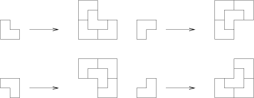
Figure 1. The chair substitution

A second example involves the 2-dimensional chair substitution, illustrated in Figure 1. There are four species of L-shaped tiles, which we label by the piece of the $\displaystyle 2\times 2$ square that is missing. That is, the first tile listed in Figure 1 is NE (northeast), the second is SE, the third is SW, and the last is NW. We consider three mass distributions, shown in Figure 2:

1. $\displaystyle f_{1}$ assigns mass 2 to NE tiles, and mass 0 to NW, SW, and SE tiles.

2. $\displaystyle f_{2}$ assigns mass 1 to NE and SW tiles, and mass 0 to NW and SE tiles.

3. $\displaystyle f_{3}$ assigns mass 0 to NE and SW tiles, and mass 1 to NW and SE tiles.

As before, we ask which transports between $\displaystyle f_{1}$, $\displaystyle f_{2}$ and $\displaystyle f_{3}$ can be done in a bounded, weakly PE, or strongly PE manner.

Figure 2. Three different mass distributions on a patch of the chair tiling

We convert these questions to questions of cohomology. Since much is already known about the cohomology of tiling spaces ([4, 10, 21, 30, 31, 32, 35]), this reduces many problems of transport either to a simple look-up or to calculations using well-established techniques [6, 5, 22, 23, 24, 33, 34].

We associate a class $\displaystyle[f_{i}]\in\check{H}^{n}(\Omega_{\bf T},{\mathbb{R}})$, the top real-valued Čech cohomology of the continuous hull $\displaystyle\Omega_{\bf T}$ of $\displaystyle{\bf T}$, to each mass distribution $\displaystyle f_{i}$. We will define subspaces of $\displaystyle\check{H}^{n}(\Omega_{\bf T},{\mathbb{R}})$, called “asymptotically negligible” and “well-balanced” classes, and show that:

Theorem 1.3.

Let $\displaystyle[f_{1}]$ and $\displaystyle[f_{2}]$ be the classes in $\displaystyle\check{H}^{n}(\Omega,{\mathbb{R}})$ associated to the strongly PE mass distributions $\displaystyle f_{1}$ and $\displaystyle f_{2}$. Then

1. There exists a bounded transport from $\displaystyle f_{1}$ to $\displaystyle f_{2}$ if and only if $\displaystyle[f_{1}]-[f_{2}]$ is well-balanced.

2. There exists a weakly PE transport from $\displaystyle f_{1}$ to $\displaystyle f_{2}$ if and only if $\displaystyle[f_{1}]-[f_{2}]$ is asymptotically negligible.

3. There exists a strongly PE transport from $\displaystyle f_{1}$ to $\displaystyle f_{2}$ if and only if $\displaystyle[f_{1}]=[f_{2}]$.

There are many examples of non-zero classes that are asymptotically negligible, leading to mass distributions that admit weakly PE transport but not strongly PE transport. In particular, we will see that the Fibonacci example admits weakly PE but not strongly PE transport from $\displaystyle f_{1}$ to $\displaystyle f_{2}$.

Conjecture 1.4.

Let $\displaystyle{\bf T}$ be an arbitrary tiling that is repetitive and has finite local complexity. Then every well-balanced class in $\displaystyle H^{n}(\Omega_{\bf T},{\mathbb{R}})$ is asymptotically negligible.

In a subsequent paper we will address this conjecture, and its generalization to classes in $\displaystyle H^{k}(\Omega_{\bf T},{\mathbb{R}})$ with $\displaystyle k<n$, in the context of substitution tilings [25].

In this paper we prove

Theorem 1.5.

Let $\displaystyle{\bf T}$ be a repetitive and aperiodic tiling of $\displaystyle{\mathbb{R}}^{n}$. If

• $\displaystyle n=1$, or

• $\displaystyle{\bf T}$ is a codimension-1 cut-and-project tiling with canonical window,

then every well-balanced class in $\displaystyle\check{H}^{n}(\Omega_{\bf T},{\mathbb{R}})$ is asymptotically negligible. In particular, given strongly PE mass distributions $\displaystyle f_{1}$ and $\displaystyle f_{2}$, there exists a bounded transport from $\displaystyle f_{1}$ to $\displaystyle f_{2}$ if and only if there exists a weakly PE transport from $\displaystyle f_{1}$ to $\displaystyle f_{2}$.

In Section 2 we review the formalism of aperiodic tilings, continuous hulls, Čech cohomology and PE cohomology, and we precisely define what it means for a class in $\displaystyle\check{H}^{n}(\Omega_{\bf T},{\mathbb{R}})$ to be well-balanced or asymptotically negligible. In Section 3 we give a cohomological interpretation of the problem of PE transport, and prove Theorem 1.3. We then use Theorem 1.3 to solve the Fibonacci and chair examples. In Section 4 we prove a slightly more general version of Theorem 1.5.

2. Background

In this section we go over the general formalism of tilings and tiling cohomology. For details, see ([31], Chapters 1 and 3).

A tile is a topological ball in $\displaystyle{\mathbb{R}}^{n}$, equal to the closure of its interior, and equipped with a label. A tiling is a set of tiles whose union is all of $\displaystyle{\mathbb{R}}^{n}$, such that tiles only intersect on their boundaries. If $\displaystyle t$ is a tile and $\displaystyle x\in{\mathbb{R}}^{n}$, then $\displaystyle t-x$ is a tile, with the same label as $\displaystyle t$, obtained by translating all the points of $\displaystyle t$ by $\displaystyle-x$. Two tiles $\displaystyle t_{1}$ and $\displaystyle t_{2}$ are translationally equivalent if $\displaystyle t_{2}=t_{1}-x$ for some $\displaystyle x\in{\mathbb{R}}^{n}$. The equivalence classes of this relation are called prototiles. A patch is a finite set of tiles in a tiling, and $\displaystyle{\mathbb{R}}^{n}$ acts on patches by moving each tile separately.

If $\displaystyle K$ is a compact set and $\displaystyle{\bf T}$ is a tiling, let $\displaystyle[K]_{\bf T}$ denote the patch of tiles in $\displaystyle{\bf T}$ that intersects $\displaystyle K$. We assume that our tilings have finite local complexity, or FLC. This means that for any $\displaystyle K$, the set $\displaystyle\{[K-x]_{\bf T}|x\in{\mathbb{R}}^{n}\}$ is finite up to translation. This is equivalent to there are being finitely many prototiles, and finitely many ways that two tiles can touch, up to translation.

Let $\displaystyle B_{R}(x)$ denote the closed ball of radius $\displaystyle R$ around a point $\displaystyle x\in{\mathbb{R}}^{n}$. If $\displaystyle{\bf T}_{1}$ and $\displaystyle{\bf T}_{2}$ are two FLC tilings, we say that $\displaystyle{\bf T}_{2}$ is locally derivable from $\displaystyle{\bf T}_{1}$ if there exists a radius $\displaystyle R$ such that $\displaystyle[B_{R}(0)]_{{\bf T}_{1}-x}=[B_{R}(0)]_{{\bf T}_{1}-y}$, then $\displaystyle[B_{1}(0)]_{{\bf T}_{2}-x}=[B_{1}(0)]_{{\bf T}_{2}-y}$. That is, the pattern of $\displaystyle{\bf T}_{2}$ in a ball of radius 1 around $\displaystyle x$ (i.e. the pattern of $\displaystyle{\bf T}_{2}-x$ in a ball of radius 1 around the origin) is determined exactly by the pattern of $\displaystyle{\bf T}_{1}$ is a ball of radius $\displaystyle R$ around $\displaystyle x$. If $\displaystyle{\bf T}_{2}$ is locally derivable from $\displaystyle{\bf T}_{1}$ and $\displaystyle{\bf T}_{1}$ is locally derivable from $\displaystyle{\bf T}_{2}$, we say that $\displaystyle{\bf T}_{1}$ and $\displaystyle{\bf T}_{2}$ are mutually locally derivable, or MLD.

We can also speak of labeled point patterns being locally derivable from tilings, or vice-versa. A discrete point pattern $\displaystyle X$ (with each point being assigned one of a finite set of labels) is locally derived from $\displaystyle{\bf T}$ if there exists an $\displaystyle R>0$ such that $\displaystyle[B_{R}(0)]_{{\bf T}-x}=[B_{R}(0)]_{{\bf T}-y}$, then $\displaystyle B_{1}(0)\cap{X-x}=B_{1}(0)\cap{X-y}$. Conversely, $\displaystyle{\bf T}$ is locally derived from $\displaystyle X$ if there exists an $\displaystyle R>0$ such that, whenever $\displaystyle B_{R}(0)\cap{X-x}=B_{R}(0)\cap{X-y}$, $\displaystyle[B_{1}(0)]_{{\bf T}-x}=[B_{R}(1)]_{{\bf T}-y}$. A point pattern $\displaystyle X_{2}$ is locally derived from $\displaystyle X_{1}$ if there exists an $\displaystyle R>0$ such that, whenever $\displaystyle B_{R}(0)\cap{X_{1}-x}=B_{R}(0)\cap{X_{1}-y}$, $\displaystyle B_{1}(0)\cap{X_{2}-x}=B_{1}(0)\cap{X_{2}-y}$.

Given a tiling, the set of vertices of that tiling, with appropriate labels for the vertices, is MLD to the original tiling. Given a point pattern, the set of Voronoi cells of that point pattern, with appropriate vertices, is MLD to the point pattern. By combining these two operations, we see that every FLC tiling is MLD to a tiling by convex polytopes that meet full-face to full-face.

Given a set of prototiles, there is a metric on the space of tilings by those prototiles. Two FLC tilings $\displaystyle{\bf T}_{1}$, $\displaystyle{\bf T}_{2}$ are $\displaystyle\epsilon$-close if there exist $\displaystyle x_{1},x_{2}\in{\mathbb{R}}^{n}$ with $\displaystyle|x_{i}|<\epsilon$, such that $\displaystyle[B_{1/\epsilon}(0)]_{{\bf T}_{1}-x_{1}}=[B_{1/\epsilon}(0)]_{{\bf T}_{2}-x_{2}}$. That is, two tilings are close if they agree on a large ball up to a small translation. The continuous hull $\displaystyle\Omega_{\bf T}$ of a tiling $\displaystyle{\bf T}$ is the completion of the translational orbit $\displaystyle\{{\bf T}-x\}$. A tiling $\displaystyle{\bf T}^{\prime}$ is in $\displaystyle\Omega_{\bf T}$ if and only if every patch of $\displaystyle{\bf T}^{\prime}$ is a translate of a patch of $\displaystyle{\bf T}$.

An FLC tiling $\displaystyle{\bf T}$ is repetitive if for every patch $\displaystyle P$ of $\displaystyle{\bf T}$ there exists a radius $\displaystyle R$ such that every ball of radius $\displaystyle R$ in $\displaystyle{\bf T}$ contains at least one occurrence of $\displaystyle P$. An FLC tiling $\displaystyle{\bf T}$ is repetitive if and only if the hull $\displaystyle\Omega_{\bf T}$ is a minimal dynamical system, i.e. if all tilings in $\displaystyle\Omega_{\bf T}$ exhibit the same set of patches (up to translation).

A tiling $\displaystyle{\bf T}$ is aperiodic if $\displaystyle{\bf T}-x={\bf T}$ implies $\displaystyle x=0$. If $\displaystyle{\bf T}$ is aperiodic and repetitive, then a neighborhood of $\displaystyle{\bf T}$ in $\displaystyle\Omega_{\bf T}$ is homeomorphic to the product of a Cantor set and an open subset of $\displaystyle{\mathbb{R}}^{n}$.

We henceforth assume that all tilings are FLC, aperiodic and repetitive, with tiles that are convex polytopes that meet full-face to full-face.

Given such a tiling $\displaystyle{\bf T}$, a continuous function $\displaystyle f:{\mathbb{R}}^{n}\to{\mathbb{R}}$ is said to be strongly pattern equivariant (PE) with respect to $\displaystyle{\bf T}$ if there exists a radius $\displaystyle R$ such that, whenever $\displaystyle[B_{R}(0)]_{{\bf T}-x}=[B_{R}(0)]_{{\bf T}-y}$, $\displaystyle f(x)=f(y)$. That is, $\displaystyle f$ is PE with radius $\displaystyle R$ if the value of $\displaystyle f(x)$ is determined exactly by the pattern of $\displaystyle{\bf T}$ in a ball of radius $\displaystyle R$ around $\displaystyle x$. A weakly PE function is the uniform limit of strongly PE functions of arbitrary radius. A function $\displaystyle f$ is weakly PE if for every $\displaystyle\epsilon>0$ there exists a radius $\displaystyle R_{\epsilon}$ such that the value of $\displaystyle f(x)$ is determined to within $\displaystyle\epsilon$ by the pattern of $\displaystyle{\bf T}$ in a ball of radius $\displaystyle R_{\epsilon}$ around $\displaystyle x$.

The tiling $\displaystyle{\bf T}$ gives a decomposition of $\displaystyle{\mathbb{R}}^{n}$ into 0-cells (vertices), 1-cells (edges), 2-cells (faces), etc. A $\displaystyle k$-cochain is an assignment of a real number to each $\displaystyle k$-cell. As with functions, $\displaystyle k$-cochains can be weakly or strongly PE. Let $\displaystyle\Omega^{k}({\bf T})$ be the set of strongly PE $\displaystyle k$-cochains. The coboundary of a strongly PE cochain is strongly PE (albeit possibly with a slightly larger radius), yielding a complex

(1) $$0\rightarrow\Omega^{0}({\bf T})\xrightarrow{\delta_{0}}\Omega^{1}({\bf T})\xrightarrow{\delta_{1}}\cdots\xrightarrow{\delta_{n-1}}\Omega^{n}({\bf T})\rightarrow 0.$$

Another version of pattern equivariant cohomology (in fact, the original version proposed in [21]) uses differential forms. We say that a $\displaystyle k$-form $\displaystyle\alpha$ on $\displaystyle{\mathbb{R}}^{n}$ is strongly PE if it can be written as a sum $\displaystyle\sum_{I}\alpha_{I}(x)dx^{I}$ and each coefficient function $\displaystyle\alpha_{I}$ is strongly PE. We say that $\displaystyle\alpha$ is weakly PE if each $\displaystyle\alpha_{I}$, and all derivatives of $\displaystyle\alpha_{I}$ of all orders, are weakly PE functions. The exterior derivative of a strongly PE form is strongly PE, so we can consider the complex of strongly PE forms. The key fact, due to [21] for forms and to [30] for cochains, is:

Theorem 2.1.

The cohomology of the de-Rham-like complex of strongly PE forms on $\displaystyle{\bf T}$, and the cohomology of the complex of real-valued PE cochains, are both canonically isomorphic to the real-valued Čech cohomology of the continuous hull $\displaystyle\Omega_{\bf T}$.

Note that both versions of PE cohomology depend only on the tiling space $\displaystyle\Omega_{\bf T}$ and not on the particular tiling $\displaystyle{\bf T}$ that is used for the calculations, and both are invariant under homeomorphisms of $\displaystyle\Omega_{\bf T}$. Thanks to this fact, we can use the symbol $\displaystyle\check{H}^{k}(\Omega_{\bf T},{\mathbb{R}})$ to refer the real-valued PE cohomology of $\displaystyle{\bf T}$ (using either forms or cochains), as well as to the Čech cohomology of $\displaystyle\Omega_{\bf T}$. Moreover, the isomorphism of form-based and cochain-based cohomology is easy to construct. Every class in the form-based cohomology is represented by a closed PE $\displaystyle k$-form, which can be integrated over $\displaystyle k$-cells to give a closed PE cochain, which represents a class in the cochain-based cohomology. In particular, if we have a smooth strongly PE mass density $\displaystyle f$, then we have a strongly PE $\displaystyle n$-form $\displaystyle fd^{n}x$. Integrating this form over tiles gives a strongly PE $\displaystyle n$-cochain.

Suppose that $\displaystyle\alpha$ is a strongly PE $\displaystyle n$-cochain. For dimensional reasons, $\displaystyle\delta\alpha=0$, so $\displaystyle\alpha$ represents a cohomology class in $\displaystyle\check{H}^{n}(\Omega_{\bf T},{\mathbb{R}})$. We call such a cochain well balanced if there exists constants $\displaystyle c_{1}$ and $\displaystyle c_{2}$ such that, for every patch $\displaystyle P$,

(2) $$\left|\int_{P}\alpha\right|\leq c_{1}+c_{2}|\partial P|,$$

where $\displaystyle|\partial P|$ is the $\displaystyle(n-1)$-dimensional Lebesgue measure of the boundary of $\displaystyle P$, and where $\displaystyle\int_{P}\alpha$ denotes the value of $\displaystyle\alpha$ applied to the chain $\displaystyle P$. If $\displaystyle\alpha=\delta\beta$ for some strongly PE (and therefore bounded) $\displaystyle(n-1)$-cochain $\displaystyle\beta$, then this condition is always met, since

(3) $$\int_{P}\alpha=\int_{\partial P}\beta.$$

The well-balanced condition therefore only depends on the cohomology class of $\displaystyle\alpha$, and we define $\displaystyle\check{H}^{n}_{WB}(\Omega_{\bf T},{\mathbb{R}})$ to be the classes in $\displaystyle\check{H}^{n}(\Omega_{\bf T},{\mathbb{R}})$ represented by well-balanced cochains.

If $\displaystyle\alpha$ is a strongly PE $\displaystyle n$-cochain and there exists a weakly PE $\displaystyle(n-1)$-cochain $\displaystyle\beta$ such that $\displaystyle\alpha=\delta\beta$, then we say that $\displaystyle\alpha$ is weakly exact. As before, this only depends on the cohomology class of $\displaystyle\alpha$, since if $\displaystyle\alpha^{\prime}=\alpha+\delta\gamma$, where $\displaystyle\gamma$ is a strongly PE cochain, and if $\displaystyle\alpha=\delta\beta$, where $\displaystyle\beta$ is weakly PE, then $\displaystyle\alpha^{\prime}=\delta(\gamma+\beta)$, where $\displaystyle\gamma+\beta$ is weakly PE. The cohomology class of a weakly exact cochain is said to be asymptotically negligible. We denote the asymptotically negligible classes in $\displaystyle H^{n}(\Omega_{T},{\mathbb{R}})$ by $\displaystyle\check{H}^{n}_{AN}(\Omega_{\bf T},{\mathbb{R}})$.

Proposition 2.2.

$\displaystyle\check{H}^{n}_{AN}(\Omega_{\bf T},{\mathbb{R}})\subset\check{H}^{n}_{WB}(\Omega_{\bf T},{\mathbb{R}})$.

Proof.

Suppose that $\displaystyle\alpha=\delta\beta$ with $\displaystyle\beta$ weakly PE. Since $\displaystyle\beta$ is the uniform limit of strongly PE cochains, and since strongly PE cochains are bounded, $\displaystyle\beta$ is bounded. That is, there exists a constant $\displaystyle C$ such that, for every $\displaystyle(n-1)$-cell $\displaystyle z$ in $\displaystyle{\bf T}$, $\displaystyle|\beta(z)|\leq C|z|$. But then, for every patch $\displaystyle P$,

$$\left|\int_{P}\alpha\right|=\left|\int_{\partial P}\beta\right|\leq C|\partial P|,$$

so $\displaystyle\alpha$ is well-balanced. ∎

We complete this section by considering what it means for bounded transport to be strongly or weakly PE. The situation is slightly different, depending on whether we consider points, masses concentrated at points, or countinuous distributions of mass.

There is no such thing as weakly PE transport of points. If $\displaystyle X_{1}$ and $\displaystyle X_{2}$ are discrete point patterns, each locally derived from $\displaystyle{\bf T}$, then a bounded transport $\displaystyle b:X_{1}\to X_{2}$ is strongly PE if there exists an $\displaystyle R>0$ such that, whenever $\displaystyle x,y\in X_{1}$ and $\displaystyle B_{R}(0)\cap(X_{1}-x)=B_{R}(0)\cap(X_{1}-y)$, then $\displaystyle b(x)-x=b(y)-y$. That is, the displacement $\displaystyle b(x)-x$ is determined exactly by the pattern of $\displaystyle X_{1}$ in a ball around $\displaystyle x$, which in turn is determined exactly by the pattern of $\displaystyle{\bf T}$ in a ball (of possibly bigger radius $\displaystyle R^{\prime}$) around $\displaystyle x$. However, since $\displaystyle X_{2}$ has FLC (being locally derived from the FLC tiling $\displaystyle{\bf T}$), it is impossible to approximate one bounded transport by another, so it does not make sense to speak of the bounded transport $\displaystyle b$ being weakly PE.

However, there is a more general notion of mass transfer among point masses where weak pattern equivariance does make sense. Suppose that $\displaystyle b:X_{1}\times X_{2}\to{\mathbb{R}}$, and that for $\displaystyle x_{1}\in X_{1}$ and $\displaystyle x_{2}\in X_{2}$, $\displaystyle b(x_{1},x_{2})$ represents the amount of mass transported from $\displaystyle x_{1}$ to $\displaystyle x_{2}$. This needn’t be an integer. All that is required is that $\displaystyle 0\leq b(x_{1},x_{2})\leq 1$, that for fixed $\displaystyle x_{1}$ we have $\displaystyle\sum_{x_{2}\in X_{2}}b(x_{1},x_{2})=1$, and that for fixed $\displaystyle x_{2}\in X_{2}$ we have $\displaystyle\sum_{x_{1}\in X_{1}}b(x_{1},x_{2})=1$. The transport $\displaystyle b$ is bounded if there is a constant $\displaystyle R$ such that $\displaystyle b(x_{1},x_{2})=0$ whenever $\displaystyle|x_{1}-x_{2}|>R$. The bounded transport $\displaystyle b$ is strongly PE if there is a constant $\displaystyle R^{\prime}$ such that $\displaystyle b(x_{1},x_{2})$ is determined exactly by $\displaystyle B_{R^{\prime}}(0)\cap(X_{1}-x_{1})$, and $\displaystyle b$ if weakly PE is $\displaystyle b$ is the uniform limit of strongly PE transport functions.

We also consider mass transport from one density $\displaystyle f_{1}$ to another density $\displaystyle f_{2}$. A transport function is a function $\displaystyle b:{\mathbb{R}}^{n}\times{\mathbb{R}}^{n}\to{\mathbb{R}}$, where $\displaystyle b(x,y)$ is a density of mass transported from $\displaystyle x$ to $\displaystyle y$. More precisely, if $\displaystyle A,B\subset{\mathbb{R}}^{n}$ are compact sets, then $\displaystyle\iint_{A\times B}b(x,y)d^{n}x\,d^{n}y$ is the amount of mass transported from $\displaystyle A$ to $\displaystyle B$. As with mass distributions localized at points, $\displaystyle b$ is bounded if there is a constant $\displaystyle R$ such that $\displaystyle b(x,y)=0$ whenever $\displaystyle|x-y|>R$. The transport $\displaystyle b$ is strongly PE if $\displaystyle b(x,y)$ is determined exactly by the pattern of $\displaystyle{\bf T}$ is a ball of radius $\displaystyle R^{\prime}$ around $\displaystyle x$ (equivalently, by $\displaystyle[B_{R^{\prime}}(0)]_{{\bf T}-x}$). This can be expressed in an integral form. Let $\displaystyle b_{A,B}(x,y)=\iint_{(x+A)\times(y+B)}b(x^{\prime},y^{\prime})d^{n}x^{\prime}\,d^{n}y^{\prime}$. This is the amount of mass transported from $\displaystyle x+A$ to $\displaystyle y+B$. $\displaystyle b$ is a strongly PE transport density if and only if, for arbitrary $\displaystyle A$ and $\displaystyle B$, $\displaystyle b_{A,B}$ is a strongly PE function. We say that $\displaystyle b$ is a weakly PE transport density if and only if, for arbitrary $\displaystyle A$ and $\displaystyle B$, $\displaystyle b_{A,B}$ is a weakly PE function.

3. The Cohomological Picture

Suppose that $\displaystyle X_{1}$ and $\displaystyle X_{2}$ are discrete point patterns, each locally derived from a non-periodic, repetitive FLC tiling $\displaystyle{\bf T}$. Note that $\displaystyle X_{1}$ and $\displaystyle X_{2}$ are Delone sets. Let $\displaystyle R$ be a distance such that every ball of radius $\displaystyle R$ contains at least one point from each of the two collections. Let $\displaystyle\rho$ be a bump function whose support is a ball of radius $\displaystyle R$. Let $\displaystyle f_{i}(x)=\sum_{x^{\prime}\in X_{i}}\rho(x-x^{\prime})$. This can be viewed as the convolution of $\displaystyle\rho$ with a Dirac comb supported on $\displaystyle X_{i}$.

Theorem 3.1.

If there is a bounded transport from $\displaystyle X_{1}$ to $\displaystyle X_{2}$ in the sense of point masses, then there is a bounded transport from $\displaystyle f_{1}$ to $\displaystyle f_{2}$ in the sense of density functions. Furthermore, if there exists a transport from $\displaystyle X_{1}$ to $\displaystyle X_{2}$ that is (strongly or weakly) PE, then then there exists a similarly PE transport from $\displaystyle f_{1}$ to $\displaystyle f_{2}$.

Proof.

The strategy for getting a transport from $\displaystyle f_{1}$ to $\displaystyle f_{2}$ is to first move mass by up to $\displaystyle R$ to convert $\displaystyle f_{1}$ to a collection of unit point masses at $\displaystyle X_{1}$, then to do the bounded transport from $\displaystyle X_{1}$ to $\displaystyle X_{2}$, and then to move mass by up to $\displaystyle R$ to get $\displaystyle f_{2}$.

Specifically, if $\displaystyle b_{0}:X_{1}\times X_{2}\to{\mathbb{R}}$ describes the transport from $\displaystyle X_{1}$ to $\displaystyle X_{2}$, then for $\displaystyle x,y\in{\mathbb{R}}^{n}$ we define

(4) $$b(x,y)=\sum_{x^{\prime}\in X_{1}}\sum_{y^{\prime}\in X_{2}}\rho(x-x^{\prime})\rho(y-y^{\prime})b_{0}(x^{\prime},y^{\prime}).$$

This sum is finite, since it only involves points $\displaystyle x^{\prime}$ within a distance $\displaystyle R$ of $\displaystyle x$ and points $\displaystyle y^{\prime}$ within a distance $\displaystyle r$ of $\displaystyle y$. If $\displaystyle b_{0}(x^{\prime},y^{\prime})=0$ whenever $\displaystyle|x^{\prime}-y^{\prime}|>R^{\prime}$, then $\displaystyle b(x,y)=0$ whenever $\displaystyle|x-y|>2R+R^{\prime}$. Note that

(5) $$\displaystyle\int_{{\mathbb{R}}^{n}}b(x,y)d^{n}y \displaystyle= \displaystyle\sum_{x^{\prime}\in X_{1}}\sum_{y^{\prime}\in X_{2}}\rho(x-x^{\prime})b_{0}(x^{\prime},y^{\prime})$$

(6) $$\displaystyle= \displaystyle\sum_{x^{\prime}\in X_{1}}\rho(x-x^{\prime})$$

(7) $$\displaystyle= \displaystyle f_{1}(x),$$

and similarly $\displaystyle\int b(x,y)d^{n}x=f_{2}(y)$. If $\displaystyle b_{0}$ is strongly PE with radius $\displaystyle R^{\prime\prime}$, then $\displaystyle b$ is strongly PE with radius $\displaystyle 2R+R^{\prime\prime}$. If $\displaystyle b_{0}$ is weakly PE, then $\displaystyle b$ is weakly PE. ∎

The reverse implication is less immediate, since there isn’t a canonical way to convert a continuous distribution into a point pattern. We’ll return to this question later.

We now relate transport of continuous distributions to cohomology. If $\displaystyle f_{1}$ and $\displaystyle f_{2}$ are strongly PE mass densities, let $\displaystyle\alpha_{i}$ be a (strongly PE) cochain whose value on a tile is the integral of $\displaystyle f_{i}d^{n}x$ over that tile. Let $\displaystyle[f_{1}]$ and $\displaystyle[f_{2}]$ be the cohomology classes of $\displaystyle\alpha_{1}$ and $\displaystyle\alpha_{2}$, respectively.

Theorem 3.2.

There is a bounded transport from $\displaystyle f_{1}$ to $\displaystyle f_{2}$ if and only if there exists a bounded $\displaystyle(n-1)$-cochain $\displaystyle\beta$ such that $\displaystyle\delta\beta=\alpha_{1}-\alpha_{2}$. Furthermore, the transport from $\displaystyle f_{1}$ to $\displaystyle f_{2}$ can be chosen to be (strongly or weakly) PE if and only if $\displaystyle\beta$ can be chosen to be (strongly or weakly) PE.

Proof.

If there is a transport from $\displaystyle f_{1}$ to $\displaystyle f_{2}$, let $\displaystyle\beta$ on a tile face be the minus the net mass transported across that face (say along a straight line). $\displaystyle\delta\beta$ applied to a tile is minus the sum of the transfers on all of its faces, i.e. minus the change in mass, so $\displaystyle\delta\beta=\alpha_{1}-\alpha_{2}$. If the transport is bounded by a distance $\displaystyle R$, then the mass transported across a face is bounded by the total existing mass within $\displaystyle R$ of that face, so $\displaystyle\beta$ is bounded. Likewise, if the transport is pattern-equivariant, then so is $\displaystyle\beta$.

For the converse, we assign a point $\displaystyle p(t)$ to each tile $\displaystyle t$ (in a strongly PE way) and do a bounded transport to put all the mass $\displaystyle\alpha_{1}(t)$ of the tile $\displaystyle t$ at that point. Given a bounded cochain $\displaystyle\beta$ with $\displaystyle\delta\beta=\alpha_{1}-\alpha_{2}$, we will construct a bounded transport that converts this collection of point masses into a collection of point masses of size $\displaystyle\alpha_{2}(t)$ at each $\displaystyle p(t)$. By Theorem 3.1 (or more precisely, by the proof of the theorem adapted to the case where the points do not have unit mass), this implies the existence of a bounded transport from $\displaystyle f_{1}$ to $\displaystyle f_{2}$.

Since each $\displaystyle f_{i}$ is positive, there is a lower bound $\displaystyle\epsilon>0$ to the value of $\displaystyle\alpha_{i}$ on any tile. There is also an upper bound $\displaystyle N_{1}$ to the number of faces a tile can have. Let $\displaystyle N_{2}$ be an upper bound to the values of $\displaystyle|\beta(c)|$, and let $\displaystyle N_{3}=\lceil MN/\epsilon\rceil$, so that $\displaystyle|\beta(c)|/N_{3}<\epsilon/N_{1}$. We do our mass transport in $\displaystyle N_{3}$ steps, in each step transferring mass $\displaystyle-\beta(c)/N_{3}$ across the face $\displaystyle c$. At every step, the mass in each tile $\displaystyle t$ is a weighted average of $\displaystyle\alpha_{1}(t)$ and $\displaystyle\alpha_{2}(t)$, and so is at least $\displaystyle\epsilon$, so there is enough mass in each tile to do the transfer. At each step, each piece of mass is moved a distance at most twice the diameter of the largest tile, so the $\displaystyle N_{3}$-step transfer process is bounded.

If $\displaystyle\beta$ is (weakly or strongly) PE, then the transfer at each step from point masses of size $\displaystyle\alpha_{1}(t)$ to point masses of size $\displaystyle\alpha_{2}(t)$ is (weakly or strongly) PE, making the entire process (weakly of strongly) PE. ∎

Proof of Theorem 1.3.

Statement 1: If there exists a bounded $\displaystyle\beta$, then $\displaystyle[f_{1}]-[f_{2}]$ is well-balanced, since for any patch $\displaystyle P$, $\displaystyle\left|\int_{P}(f_{1}(x)-f_{2}(x))d^{n}x\right|=\left|\int_{P}\alpha_{1}-\alpha_{2}\right|=\left|\int_{\partial P}\beta\right|\leq\hbox{const. }|\partial P|.$

Conversely, if $\displaystyle[f_{1}]-[f_{2}]$ is well-balanced, then $\displaystyle\left|\int_{P}(f_{1}-f_{2})d^{n}x\right|=\left|\int_{P}\alpha_{1}-\alpha_{2}\right|$ is bounded by a fixed multiple of $\displaystyle|\partial P|$. Since there are lower bounds to the densities $\displaystyle f_{1}$ and $\displaystyle f_{2}$, there is a constant $\displaystyle r_{0}$ (independent of $\displaystyle P$) such that the integrals of $\displaystyle f_{1}$ and $\displaystyle f_{2}$ over every region of area at least $\displaystyle r_{0}|\partial P|$ are both greater than $\displaystyle\left|\int_{P}(f_{1}-f_{2})d^{n}x\right|$. This implies that there is an $\displaystyle r$ (of the same order as $\displaystyle r_{0}$, but whose precise derivation requires some geometrical arguments) such that the integral of $\displaystyle f_{1}$ over every $\displaystyle r$-neighborhood of $\displaystyle P$ is greater than the integral of $\displaystyle f_{2}$ over $\displaystyle P$, and such that the integral of $\displaystyle f_{2}$ over the $\displaystyle r$-neighborhood is greater than the integral of $\displaystyle f_{1}$ over $\displaystyle P$. By the Hall Marriage Theorem (see also [29]) this implies the existence of a bounded transport from $\displaystyle f_{1}$ to $\displaystyle f_{2}$.

Statement 2: By Theorem 3.2, there exists a weakly PE transport from $\displaystyle f_{1}$ to $\displaystyle f_{2}$ if and only if there exists a weakly PE cochain $\displaystyle\beta$ such that $\displaystyle\delta\beta=\alpha_{1}-\alpha_{2}$. But by definition, that is the same as $\displaystyle[f_{1}]-[f_{2}]$ being asymptotically negligible.

Statement 3: By Theorem 3.2, there exists a strongly PE transport from $\displaystyle f_{1}$ to $\displaystyle f_{2}$ if and only if there exists a strongly PE cochain $\displaystyle\beta$ such that $\displaystyle\delta\beta=\alpha_{1}-\alpha_{2}$. But by definition, that is the same as $\displaystyle\alpha_{1}$ being cohomologous to $\displaystyle\alpha_{2}$, in other words of $\displaystyle[f_{1}]-[f_{2}]$ being zero. ∎

We now return to our example problems. In the Fibonacci tiling, $\displaystyle H^{1}(\Omega_{T},{\mathbb{R}})={\mathbb{R}}^{2}$. $\displaystyle H^{1}_{AN}$ is the contractive subspace of $\displaystyle H^{1}$ under substitution [6], which is 1-dimensional, so $\displaystyle H^{1}(\Omega_{T},{\mathbb{R}})={\mathbb{R}}\oplus H^{1}_{AN}(\Omega_{T},{\mathbb{R}})$. In particular, any two classes with the same overall density differ by an asymptotically negligible class, so $\displaystyle[f_{1}-f_{2}]$ is asymptotically negligible, so it is possible to do a weakly PE transport from $\displaystyle f_{1}$ to $\displaystyle f_{2}$.

However, it is not possible to do a strongly PE transport from $\displaystyle f_{1}$ to $\displaystyle f_{2}$. To see this, suppose that $\displaystyle f_{1}-f_{2}=\delta\beta$, where $\displaystyle\beta$ is a strongly PE function on vertices, say with radius $\displaystyle R$. By repetitivity, there are two vertices $\displaystyle v_{1}$, $\displaystyle v_{2}$ whose patterns agree to radius $\displaystyle R$. But then

(8) $$\int_{v_{1}}^{v_{2}}f_{1}-\int_{v_{1}}^{v_{2}}f_{2}=\int_{v_{1}}^{v_{2}}\delta\beta=\beta(v_{2})-\beta(v_{1})=0.$$

However, $\displaystyle\int_{v_{1}}^{v_{2}}f_{1}$ is an integer, while $\displaystyle\int_{v_{1}}^{v_{2}}f_{1}$ is a multiple of $\displaystyle\phi$, so these integrals cannot be equal. Contradiction.

Next consider the chair tiling. $\displaystyle H^{2}(\Omega_{T},{\mathbb{R}})$ is known to equal $\displaystyle{\mathbb{R}}^{3}$, and the three generators are described as follows. For $\displaystyle t\in\{NE,NW,SE,SW\}$, let $\displaystyle i_{t}$ be the indicator function of that tile, i.e. a cochain that evaluates to 1 on every $\displaystyle t$ tile and 0 on the other three kinds.

1. One generator is the constant cochain $\displaystyle i_{NE}+i_{NW}+i_{SE}+i_{SW}$ that simply counts tiles. This generator quadruples under substitution.

2. One generator is $\displaystyle i_{NE}-i_{SW}$, which is the same as $\displaystyle f_{1}-f_{2}$. It doubles under substitution, and we will soon see that it is neither WE nor WB.

3. The third generator is a rotated version of the second, namely $\displaystyle i_{NW}-i_{SE}$. It, too, is neither WE nor WB.

4. The cochain $\displaystyle i_{NE}+i_{SW}-i_{NW}-i_{SE}$ evaluates to 0 on every substituted tile, and is cohomologically trivial.

Since $\displaystyle f_{2}-f_{3}=i_{NE}+i_{SW}-i_{NW}-i_{SE}$ is exact, there exists strongly PE transport from $\displaystyle f_{2}$ to $\displaystyle f_{3}$, namely rearranging the mass within each once-substituted tile. Since $\displaystyle f_{1}-f_{2}$ (and hence $\displaystyle f_{1}-f_{3}$) is not WB, there is no bounded transport from $\displaystyle f_{1}$ to $\displaystyle f_{2}$ (or $\displaystyle f_{3}$).

Figure 3. The mass of a partial supertile grows faster than perimeter

To see that $\displaystyle\alpha=i_{NE}-i_{SW}$ is not WB, note that $\displaystyle\alpha$ doubles under substitution, and therefore evaluates to $\displaystyle 2^{m}$ on an $\displaystyle m$-substituted $\displaystyle NE$ tile, also known as an $\displaystyle m$-supertile. That is, the total mass grows like the perimeter for complete $\displaystyle m$-supertiles. Now let $\displaystyle R_{n}$ be the portion of an $\displaystyle n$-supertile of type NE obtained by cutting along a diagonal line as in Figure 3 and discarding the tiles that straddle the dividing line. $\displaystyle R_{n}$ can be subdivided into one $\displaystyle(n-1)$-supertile, three $\displaystyle(n-2)$-supertiles, seven $\displaystyle(n-3)$-supertiles, $\displaystyle\ldots$, and $\displaystyle 2^{n}-1$ ordinary tiles, all of type $\displaystyle NE$. We then have

(9) $$\int_{R_{n}}\alpha=2^{n-1}+3\times 2^{n-2}+\cdots+(2^{n}-1)\times 2^{0}=(n-1)\times 2^{n}+1.$$

Since $\displaystyle n$ is arbitrary and $\displaystyle|\partial R_{n}|=4\times 2^{n}$, $\displaystyle\int_{R_{n}}\alpha$ cannot be bounded by a uniform constant times $\displaystyle|\partial R_{n}|$.

Note that we have done more than simply solve our example puzzle. We have shown that for the chair tiling, $\displaystyle H^{2}_{WB}(\Omega_{\bf T},{\mathbb{R}})$ is trivial. Given any two strongly PE mass distributions $\displaystyle f$ and $\displaystyle g$ on a chair tiling, there exists a bounded transport from $\displaystyle f$ to $\displaystyle g$ if and only if $\displaystyle[f-g]=0$, in which case there exists a strongly PE transport from $\displaystyle f$ to $\displaystyle g$.

4. Theorem 1.5

In the last section we showed that the question: “If a bounded transport exists between two strongly PE mass distributions $\displaystyle f_{1}$ and $\displaystyle f_{2}$, does there necessarily exist a weakly PR transport?”, is equivalent to “Is every well-balanced class is $\displaystyle\check{H}^{n}(\Omega_{\bf T},{\mathbb{R}})$ asymptotically negligible”? In this section we generalize the cohomological question and then give positive answers in two settings. Theorem 1.5 then follows as a corollary.

The tiling $\displaystyle{\bf T}$ defines a decomposition of $\displaystyle{\mathbb{R}}^{n}$ into 0-cells (vertices), 1-cells (edges), 2-cells (faces), etc. Let $\displaystyle\{c^{(k)}_{i}\}$ denote the set of $\displaystyle k$-cells of the tiling, and pick an orientation for each cell. (For vertices and $\displaystyle n$-cells there is a canonical choice of orientation, but in the intermediate dimensions we must make some arbitrary choices.) A $\displaystyle k$-chain $\displaystyle A_{k}$ is a finite linear combination $\displaystyle\sum_{i}a_{i}c^{(k)}_{i}$, and we define $\displaystyle|A_{k}|=\sum_{i}|a_{i}||c^{(k)}_{i}|$, where $\displaystyle|c^{(k)}_{i}|$ is the $\displaystyle k$-dimensional Euclidean measure of $\displaystyle c^{(k)}_{i}$. If $\displaystyle\alpha$ is a $\displaystyle k$-cochain, then we write $\displaystyle\int_{c^{(k)}_{i}}\alpha$ to denote the value of $\displaystyle\alpha$ on the cell $\displaystyle c^{(k)}_{i}$, and $\displaystyle\int_{A_{k}}\alpha:=\sum_{i}a_{i}\int_{c^{(k)}_{i}}\alpha$.

We say that a strongly PE $\displaystyle k$-cochain $\displaystyle\alpha$ is well-balanced (WB) if there exists a constant $\displaystyle K$ such that, for any $\displaystyle k$-chain $\displaystyle A_{k}$, $\displaystyle\left|\int_{A_{k}}\alpha\right|\leq K|A_{k}|$. We say that $\displaystyle\alpha$ is weakly exact (WE), and that the class of $\displaystyle\alpha$ is asymptotically negligible (AN) if there exists a weakly PE $\displaystyle(k-1)$-cochain $\displaystyle\beta$ such that $\displaystyle\alpha=\delta\beta$. These properties were previously defined for $\displaystyle n$-cochains, but in fact the definitions make sense for any $\displaystyle k$. Stokes Theorem says that $\displaystyle WE\implies WB$. The question is whether $\displaystyle WB\implies WE$.

Proposition 4.1.

Every WE or WB cochain is closed.

Proof.

If $\displaystyle\alpha$ is WE, then $\displaystyle\alpha=\delta\beta$, so $\displaystyle\delta\alpha=\delta^{2}\beta=0$, so $\displaystyle\alpha$ is closed.

Next suppose that $\displaystyle\alpha$ is WB but not closed. Since $\displaystyle\alpha$ is not closed, there exists a chain $\displaystyle A_{k}$ such that $\displaystyle\partial A_{k}=0$ but $\displaystyle\int_{A_{k}}\alpha\neq 0$. But then $\displaystyle\left|\int_{A_{k}}\alpha\right|$ is not bounded by $\displaystyle K|\partial A_{k}|$, so $\displaystyle\alpha$ is not WB. Contradiction. ∎

Since the coboundaries of strongly PE cochains are both WE and WB, cohomologous cochains are either both WE or neither WE, and are either both WB or neither. We can therefore speak of a cohomology class being AN or WB, and define subspaces $\displaystyle\check{H}^{k}_{AN}(\Omega_{\bf T},{\mathbb{R}})$ and $\displaystyle\check{H}^{k}_{WB}(\Omega_{\bf T},{\mathbb{R}})$ of $\displaystyle\check{H}^{k}(\Omega_{\bf T},{\mathbb{R}})$.

The situation when $\displaystyle k=1$ is simple:

Theorem 4.2.

If $\displaystyle{\bf T}$ is a repetitive aperiodic tiling of $\displaystyle{\mathbb{R}}^{n}$ with FLC, then every strongly PE and WB 1-cochain is WE.

Proof.

When $\displaystyle n=1$ this is a special case of the classical Gottschalk-Hedlund theorem [11]. Many generalization for higher-dimensional actions have been proven over the years. A proof of this specific situation can be found in [22]. ∎

The situation when $\displaystyle k=0$ is even simpler. The only WB cochain is the zero cochain, which is WE.

A stepped plane is a canonical projection tiling from 3 to 2 dimensions. We use the term more generally for a canonical projection tiling from $\displaystyle{\mathbb{R}}^{n+1}$ to $\displaystyle{\mathbb{R}}^{n}$. Recall that an $\displaystyle m$ to $\displaystyle n$ dimensional projection tiling is canonical if the window in the internal space $\displaystyle{\mathbb{R}}^{m-n}$ is the projection of a unit cube in $\displaystyle{\mathbb{R}}^{m}$.

Theorem 4.3.

Let $\displaystyle{\bf T}$ be a stepped plane in $\displaystyle{\mathbb{R}}^{n}$, and let $\displaystyle\alpha$ represent a strongly PE and WB class in $\displaystyle\check{H}^{k}(\Omega_{\bf T},{\mathbb{R}})$. Then $\displaystyle\alpha$ is WE.

Proof.

Since $\displaystyle{\bf T}$ is a canonical cut-and-project tiling from $\displaystyle n+1$ to $\displaystyle n$ dimensions, the window for the projection is an interval whose endpoints correspond to the same hyperplane $\displaystyle H$ in the torus $\displaystyle T={\mathbb{R}}^{n+1}/{\mathbb{Z}}^{n+1}$. As a topological space, $\displaystyle\Omega_{\bf T}$ is then obtained from $\displaystyle T$ by removing $\displaystyle H$ and gluing in two copies of $\displaystyle H$, each representing a limit from one side. The Čech cohomology of $\displaystyle\Omega_{\bf T}$ is then isomorphic to the cohomology of $\displaystyle T$ with one point removed. That is, $\displaystyle\check{H}^{k}(\Omega_{\bf T},{\mathbb{R}})$ is isomorphic to $\displaystyle H^{k}(T,{\mathbb{R}})$ for $\displaystyle k=0,\ldots,n$. In particular, $\displaystyle\check{H}^{*}(\Omega_{\bf T},{\mathbb{R}})$ is freely generated as an exterior algebra, in dimensions up through $\displaystyle n$, by $\displaystyle\check{H}^{1}(\Omega_{\bf T},{\mathbb{R}})$.

Kellendonk and Sadun [23] proved that, for $\displaystyle m$-to-$\displaystyle n$ dimensional cut-and-project tilings with polyhedral windows, $\displaystyle\dim\check{H}^{1}_{AN}(\Omega_{\bf T},{\mathbb{R}})=m-n$. For stepped planes, this means that we can choose a basis for $\displaystyle\check{H}^{1}(\Omega_{\bf T},{\mathbb{R}})$ such that one basis element can be represented, using the de Rham version of cohomology, by a form $\displaystyle df$, where $\displaystyle f$ is a weakly PE function, and that the other $\displaystyle n$ basis elements can be represented the constant forms $\displaystyle dx^{i}$. A basis for $\displaystyle\check{H}^{k}$ is then given by the forms $\displaystyle dx^{I}:=dx^{i_{1}}\wedge\cdots\wedge dx^{i_{k}}$ for multiindices $\displaystyle I=\{i_{1},\ldots,i_{k}\}$, and $\displaystyle df\wedge dx^{J}$ for multiindices $\displaystyle J=\{j_{1},\ldots,j_{k-1}\}$.

Note that $\displaystyle df\wedge dx^{J}=d(fdx^{J})$ is WE, and hence WB, while $\displaystyle dx^{I}$ (and all nonzero linear combinations of the $\displaystyle dx^{I}$’s) is not WB, and hence not WE. This implies that $\displaystyle\check{H}^{k}_{AN}(\Omega_{\bf T},{\mathbb{R}})$ and $\displaystyle\check{H}^{k}_{WB}(\Omega_{\bf T},{\mathbb{R}})$ are both the span of the $\displaystyle df\wedge dx^{J}$’s, and hence are equal. ∎

Theorem 1.5 is just the $\displaystyle k=n$ case of Theorems 4.2 and 4.3.

5. Concluding Remarks

There has been a burst of activity in recent years studying the bounded displacement (BD) equivalence relation for tilings and Delone sets [16, 19, 17, 18, 24, 1, 39, 38]. As we reported in our previous paper [24], there are many relevant papers contributing to the subject that predate the terminology BD such as [7, 8, 26]. The papers [7, 8] in particular make the connection to quasicrystals explicit. They studied the question of when a cut-and-project set is BD to a crystal. When a mathematical quasicrystal can be written as a small perturbation of a mathematical crystal (via a BD mapping), then it may be possible that the quasicrystal can be constructed from the crystal by a displacive phase transition. A closely related notion to BD is that of a bounded remainder set (BRS). There has been quite a bit of activity (including new cohomological work) in this subject area in recent years [14, 13, 12, 19, 17, 27, 24].

In a recent work [9] proved many analogues of the Euclidean results on the BD and BL equivalence relations for connected and simply connected nilpotent Lie groups (with respect to both the Riemannian and Carnot-Carthéodory metrics. Note that these groups are topologically Euclidean.). The results in [9] seem to indicate that Euclidean methods are fairly adaptable to the nilpotent setting, as far as BD is concerned. However, we are not aware of any work on the cohomology of tiling spaces for such groups. It would be interesting if the results of the present article had analogues in connected simply connected nilpotent Lie groups.

References

• [1] Faustin Adiceam, David Damanik, Franz GΓ€hler, Uwe Grimm, Alan Haynes, Antoine Julien, AndrΓ©s Navas, Lorenzo Sadun, and Barak Weiss. Open problems and conjectures related to the theory of mathematical quasicrystals. Arnold Math. J., 2(4):579–592, 2016.
• [2] JosΓ© Aliste-Prieto, Daniel Coronel, and Jean-Marc Gambaudo. Rapid convergence to frequency for substitution tilings of the plane. Comm. Math. Phys., 306(2):365–380, 2011.
• [3] JosΓ© Aliste-Prieto, Daniel Coronel, and Jean-Marc Gambaudo. Linearly repetitive Delone sets are rectifiable. Ann. Inst. H. PoincarΓ© Anal. Non LinΓ©aire, 30(2):275–290, 2013.
• [4] JaredΒ E. Anderson and IanΒ F. Putnam. Topological invariants for substitution tilings and their associated $\displaystyle C^{*}$-algebras. Ergodic Theory Dynam. Systems, 18(3):509–537, 1998.
• [5] Alex Clark and Lorenzo Sadun. When size matters: subshifts and their related tiling spaces. Ergodic Theory Dynam. Systems, 23(4):1043–1057, 2003.
• [6] Alex Clark and Lorenzo Sadun. When shape matters: deformations of tiling spaces. Ergodic Theory Dynam. Systems, 26(1):69–86, 2006.
• [7] Michel Duneau and Christophe Oguey. Displacive transformations and quasicrystalline symmetries. J. Physique, 51(1):5–19, 1990.
• [8] Michel Duneau and Christophe Oguey. Bounded interpolations between lattices. J. Phys. A, 24(2):461–475, 1991.
• [9] Tullia Dymarz, Michael Kelly, Sean Li, and Anton Lukyanenko. Separated nets in nilpotent groups. Ind. Univ. Math. Jour., 2018.
• [10] Alan Forrest, John Hunton, and Johannes Kellendonk. Topological invariants for projection method patterns. Mem. Amer. Math. Soc., 159(758):x+120, 2002.
• [11] WalterΒ Helbig Gottschalk and GustavΒ Arnold Hedlund. Topological dynamics. American Mathematical Society Colloquium Publications, Vol. 36. American Mathematical Society, Providence, R. I., 1955.
• [12] Sigrid Grepstad and Nir Lev. Universal sampling, quasicrystals and bounded remainder sets. C. R. Math. Acad. Sci. Paris, 352(7-8):633–638, 2014.
• [13] Sigrid Grepstad and Nir Lev. Sets of bounded discrepancy for multi-dimensional irrational rotation. Geom. Funct. Anal., 25(1):87–133, 2015.
• [14] Sigrid Grepstad and Nir Lev. Riesz bases, Meyer’s quasicrystals, and bounded remainder sets. Trans. Amer. Math. Soc., 370(6):4273–4298, 2018.
• [15] PaulΒ R. Halmos. Naive set theory. Springer-Verlag, New York-Heidelberg, 1974. Reprint of the 1960 edition, Undergraduate Texts in Mathematics.
• [16] Alan Haynes. Equivalence classes of codimension-one cut-and-project nets. Ergodic Theory Dynam. Systems, 36(3):816–831, 2016.
• [17] Alan Haynes, Michael Kelly, and Henna Koivusalo. Constructing bounded remainder sets and cut-and-project sets which are bounded distance to lattices, II. Indag. Math. (N.S.), 28(1):138–144, 2017.
• [18] Alan Haynes, Michael Kelly, and Barak Weiss. Equivalence relations on separated nets arising from linear toral flows. Proc. Lond. Math. Soc. (3), 109(5):1203–1228, 2014.
• [19] Alan Haynes and Henna Koivusalo. Constructing bounded remainder sets and cut-and-project sets which are bounded distance to lattices. Israel J. Math., 212(1):189–201, 2016.
• [20] Alan Haynes, Henna Koivusalo, James Walton, and Lorenzo Sadun. Gaps problems and frequencies of patches in cut and project sets. Math. Proc. Cambridge Philos. Soc., 161(1):65–85, 2016.
• [21] Johannes Kellendonk and IanΒ F. Putnam. Tilings, $\displaystyle C^{*}$-algebras, and $\displaystyle K$-theory. In Directions in mathematical quasicrystals, volumeΒ 13 of CRM Monogr. Ser., pages 177–206. Amer. Math. Soc., Providence, RI, 2000.
• [22] Johannes Kellendonk and Lorenzo Sadun. Meyer sets, topological eigenvalues, and Cantor fiber bundles. J. Lond. Math. Soc. (2), 89(1):114–130, 2014.
• [23] Johannes Kellendonk and Lorenzo Sadun. Conjugacies of model sets. Discrete Contin. Dyn. Syst., 37(7):3805–3830, 2017.
• [24] Michael Kelly and Lorenzo Sadun. Pattern equivariant cohomology and theorems of Kesten and Oren. Bull. Lond. Math. Soc., 47(1):13–20, 2015.
• [25] Michael Kelly and Lorenzo Sadun. Pattern equivariant mass transport in aperiodic tilings ii. substitutions and fragmentations. (0):0, 2018.
• [26] Harry Kesten. On a conjecture of ErdΕ‘s and SzΓΌsz related to uniform distribution $\displaystyle{\rm mod}\ 1$. Acta Arith., 12:193–212, 1966/1967.
• [27] Gady Kozma and Nir Lev. Exponential Riesz bases, discrepancy of irrational rotations and BMO. J. Fourier Anal. Appl., 17(5):879–898, 2011.
• [28] MiklΓ³sΒ Laczkovich. Equidecomposability and discrepancy; a solution of Tarski’s circle-squaring problem. J. Reine Angew. Math., 404:77–117, 1990.
• [29] MiklΓ³s Laczkovich. Uniformly spread discrete sets in $\displaystyle{\bf R}^{d}$. J. London Math. Soc. (2), 46(1):39–57, 1992.
• [30] Lorenzo Sadun. Pattern-equivariant cohomology with integer coefficients. Ergodic Theory Dynam. Systems, 27(6):1991–1998, 2007.
• [31] Lorenzo Sadun. Topology of tiling spaces, volumeΒ 46 of University Lecture Series. American Mathematical Society, Providence, RI, 2008.
• [32] Lorenzo Sadun. Cohomology of hierarchical tilings. In Mathematics of aperiodic order, volume 309 of Progr. Math., pages 73–104. BirkhΓ€user/Springer, Basel, 2015.
• [33] Lorenzo Sadun. Cohomology of hierarchical tilings. In Mathematics of aperiodic order, volume 309 of Progr. Math., pages 73–104. BirkhΓ€user/Springer, Basel, 2015.
• [34] Lorenzo Sadun. Finitely balanced sequences and plasticity of 1-dimensional tilings. Topology Appl., 205:82–87, 2016.
• [35] Lorenzo Sadun and RobertΒ F. Williams. Tiling spaces are Cantor set fiber bundles. Ergodic Theory Dynam. Systems, 23(1):307–316, 2003.
• [36] Scott Schmieding and Rodrigo TreviΓ±o. Self affine Delone sets and deviation phenomena. Comm. Math. Phys., 357(3):1071–1112, 2018.
• [37] MikhailΒ Sodin and BorisΒ Tsirelson. Uniformly spread measures and vector fields. Zap. Nauchn. Sem. S.-Peterburg. Otdel. Mat. Inst. Steklov. (POMI), 366(Issledovaniya po Lineinym Operatoram i Teorii Funktsii. 37):116–127, 130, 2009.
• [38] Yaar Solomon. Substitution tilings and separated nets with similarities to the integer lattice. Israel J. Math., 181:445–460, 2011.
• [39] Yaar Solomon. A simple condition for bounded displacement. J. Math. Anal. Appl., 414(1):134–148, 2014.
• [40] Kevin Whyte. Amenability, bi-Lipschitz equivalence, and the von Neumann conjecture. Duke Math. J., 99(1):93–112, 1999.