First passage statistics for diffusing diffusivity

Abstract

A rapidly increasing number of systems is identified in which the stochastic motion of tracer particles follows the Brownian law $\langle\mathbf{r}^{2}(t)\rangle\simeq Dt$ yet the distribution of particle displacements is strongly non-Gaussian. A central approach to describe this effect is the diffusing diffusivity (DD) model in which the diffusion coefficient itself is a stochastic quantity, mimicking heterogeneities of the environment encountered by the tracer particle on its path. We here quantify in terms of analytical and numerical approaches the first passage behaviour of the DD model. We observe significant modifications compared to Brownian-Gaussian diffusion, in particular that the DD model may have a more efficient first passage dynamics. Moreover we find a universal crossover point of the survival probability independent of the initial condition.

1 Introduction

Since its original systematic study 190 years ago by Robert Brown [1], diffusion of molecular and (sub-)micron-sized entities has been identified as the dominant form of thermally driven, passive transport in numerous biological and inanimate systems. The two hallmark features of diffusion is the linear growth $\langle\mathbf{r}^{2}(t)\rangle=2Ddt$ of the mean squared displacement (MSD) with diffusion coefficient $D$ in $d$ spatial dimensions, and the Gaussian distribution of displacements [2]. With increasing complexity of the studied systems deviations from these two central properties have been unveiled over the years. Thus, anomalous diffusion with an MSD of the form $\langle\mathbf{r}^{2}(t)\rangle\simeq t^{\alpha}$ was observed in a large range of systems [3, 4]. Along with such observations a rich variety of generalised stochastic processes has been developed [5, 6]. The displacement distribution of anomalous diffusion processes may be inherently Gaussian (such as for fractional Brownian motion [7]) or non-Gaussian (for instance, for processes characterised by scale-free trapping time distributions [8] or space-dependent diffusivity models [9]).

Recently a lage variety of systems have been reported in which the MSD exhibits the linear growth in time $\langle\mathbf{r}^{2}(t)\rangle\simeq Dt$ of Brownian (Fickian) transport, however, the distribution of displacements $P(\mathbf{r},t)$ is pronouncedly non-Gaussian [10]. Pertinent examples include the motion of tracer beads along tubular or membrane structures or in gels and colloidal suspensions [10, 11, 12], and the motion of nematodes [13] and single cells on substrates [14]. As long as the displacement distribution $P(\mathbf{r},t)$ has a fixed shape for any times $t$, one possible way to model the non-Gaussianity is the concept of superstatistics [15, 16] which introduces a distribution $p_{D}(D)$ of the diffusion coefficient and then averages individual Gaussian distributions with one given $D$ value over this $p_{D}(D)$. However, this approach does not work when eventually a crossover to an effective Gaussian is observed [10, 11]. For the latter case Chubynsky and Slater introduced the diffusing diffusivity (DD) model [17], see also [18, 19, 20, 21, 22, 23, 24]: In this popular approach the diffusion coefficient is assumed to be a stochastic variable itself, described by a stationary process. Consequently the system is initially described by a non-Gaussian displacement distribution. Beyond a characteristic time scale a crossover occurs to a Gaussian behaviour characterised by an effective value of the diffusivity.

We here study the first passage behaviour of the DD model. The concept of first passage is ubiquitously used in statistical physics and its applications, for instance, to quantify when a diffusing particle reaches a reaction centre or a stochastic process exceeds a given threshold value [25, 26]. Based on the minimal model for DD [22] we derive the first passage behaviour in both semi-infinite and finite systems. We find that the DD dynamics may outperform Brownian-Gaussian normal diffusion at intermittent times in a semi-infinite domain while the long time behaviour matches exactly the Brownian-Gaussian result with an effective diffusivity. We also observe an interesting universal crossover point of the survival probability which is independent of the initial particle position. In finite domains the mean first passage time of the DD model is longer than in the Brownian-Gaussian case. Concurrently, in the DD model the divergence of the mean first passage time observed in the superstatistical approach is rectified.

In section 2 we briefly recall the basic properties of the minimal diffusing diffusivity model [22]. The survival probabilities for the semi-infinite and finite domains are then derived in section 3 along with their short and long time asymptotes. Section 4 provides a detailed discussion of the results including a relation to the standard Brownian-Gaussian first passage behaviour. A short conclusion is presented in section 5.

2 Minimal model for Brownian yet non-Gaussian diffusion

The model we study is the so-called minimal diffusing diffusivity (DD) model which was introduced to describe diffusion in heterogeneous environments [22]. In this model the diffusivity is defined as a stochastic process itself, in terms of the squared Ornstein-Uhlenbeck process, guaranteeing the stationarity of $D(t)$. In dimensionless units the minimal DD model is defined by the set of Langevin equations [22]

$$\frac{d}{dt}\mathbf{r}(t) = \sqrt{2D(t)}{\bm{\xi}}(t)$$

$$D(t) = \mathbf{Y}^{2}(t),\quad\frac{d}{dt}\mathbf{Y}(t)=-\mathbf{Y}+{\bm{\eta}}(t),$$ (1)

where the components of $\bm{\xi}(t)$ and $\bm{\eta}(t)$ are independent white Gaussian noises and $\mathbf{Y}$ represents an $d$-dimensional Ornstein-Uhlenbeck process. The dimensionless Ornstein-Uhlenbeck process here has a characteristic crossover time of unity. We assume the diffusivity to start from equilibrium initial conditions (the non-equilibrium case is discussed in [23]). This leads to the superstatistical short time diffusivity distribution

$$p_{D}(D)=\left\{\begin{array}[]{lr}(\sqrt{\pi D})^{-1}\rme^{-D},&d=1\\ \rme^{-D},&d=2\\ (2\sqrt{D/\pi})\rme^{-D},&d=3\end{array}\right.,$$ (2)

for 1, 2 and 3 dimensions. While the dominating exponential tail is common to all $d$, there is a pole at $D\to 0$ in $d=1$ [22]. As we showed previously, the minimal DD model can be written using the concepts of subordination [27] through the relation [22]

$$P(\mathbf{r},t|\mathbf{r}_{0})=\int_{0}^{\infty}G(\mathbf{r},\tau|\mathbf{r}_{0},D=1)T_{d}(\tau,t)d\tau,$$ (3)

of the probability density function (PDF) $P(\mathbf{r},t|\mathbf{r}_{0})$ of displacement and the Gaussian

$$G(\mathbf{r},t|\mathbf{r}_{0},D)=(4\pi Dt)^{-d/2}\exp\left((\mathbf{r}-\mathbf{r}_{0})^{2}/[4Dt]\right)$$ (4)

with fixed diffusion coefficient $D$. The subordinator $T_{d}(\tau,t)$ represents the PDF of the process $\tau(t)=\int_{0}^{t}\mathbf{Y}^{2}(t^{\prime})dt^{\prime}$ and is defined through its Laplace transform [22]

$$\tilde{T}_{d}(s,t)=\exp(dt/2)\left[\frac{1}{2}(\sqrt{1+2s}+\frac{1}{\sqrt{1+2s}})\sinh\left(t\sqrt{1+2s}\right)+\cosh\left(t\sqrt{1+2s}\right)\right]^{-d/2}$$ (5)

with short and long times limits

$$\tilde{T}_{d}(s,t) \sim t^{-d/2}\left(s+1/t\right)^{-d/2}, t\ll 1,$$ (6)

$$\tilde{T}_{d}(s,t) \sim 2^{d/2}\exp\left(\frac{dt}{2}(1-\sqrt{1+2s})\right)\left(1+\frac{1}{2}\left(\sqrt{1+2s}+\frac{1}{\sqrt{1+2s}}\right)\right)^{-d/2}, t\gg 1.$$ (7)

At short times the diffusivity varies slowly and we can assume it to be almost constant. In this limit the DD model thus reduces to the superstatistical approximation of the DD model in which each particle has a constant random diffusion coefficient with distribution $p_{D}(D)$ [15, 16]: on the ensemble level this implies that the PDF can be written as $P_{\mathrm{sup}}(\mathbf{r},t|\mathbf{r}_{0})=\int_{0}^{\infty}G(\mathbf{r},t|\mathbf{r}_{0},D)p_{D}(D)dD$, such that the short time PDF explicitly reads

$$P_{\mathrm{ST}}(\mathbf{r},t|\mathbf{r}_{0})=P_{\mathrm{sup}}(\mathbf{r},t|\mathbf{r}_{0})=\left\{\begin{array}[]{lr}(\pi t^{1/2})^{-1}K_{0}\left(|x-x_{0}|/t^{1/2}\right),&d=1\\ (2\pi t)^{-1}K_{0}\left(|r-r_{0}|/t^{1/2}\right),&d=2\\ (2\pi^{2}t^{3/2})^{-1}K_{0}\left(|r-r_{0}|/t^{1/2}\right),&d=3\end{array}\right.$$ (8)

where $K_{0}(x)$ is a modified Bessel function of the second kind with exponential asymptote $K_{0}(z)\sim\sqrt{\pi/(2z)}e^{-z}$ [30]. At long times the DD process crosses over to a purely Gaussian process with PDF $P_{\mathrm{LT}}(\mathbf{r},t|\mathbf{r}_{0})=G(\mathbf{r},t|\mathbf{r}_{0},D=\langle D\rangle_{\mathrm{st}})$ with the stationary diffusivity $\langle D\rangle_{\mathrm{st}}=d/2$ [22]. For all $t$ the MSD is given by $\langle(\mathbf{r}(t)-\mathbf{r}_{0})^{2}\rangle=2d\langle D\rangle_{\mathrm{st}}t$.

We showed in [23] that there is a stochastic counterpart to this superstatistical approximation, defined through the generalised grey Brownian motion (ggBM) formalism [28], $\mathbf{r}(t)=\sqrt{2D}\times\mathbf{W}(t),$ where $D$ is the random and constant diffusion coefficient and $\mathbf{W}(t)$ is the $d$-dimensional Wiener process or standard Brownian motion. Note that while the DD model represents the heterogeneity of the medium in some mean field sense [22] the ggBM model describes an heterogeneous ensemble of particles [29] .

3 Results for the survival probabilities

The first passage time PDF of a stochastic process is the negative time derivative of the survival probability, $\wp(t)=-dS(t)/dt$. We here obtain the survival probability for semi-infinite and finite domains using the above subordination relation.

3.1 Survival of diffusing diffusivity model in semi-infinite domain

We begin our study with the semi-infinite interval $d=1$. Following the approach for standard diffusion [25] we use the method of images for the initial particle position $x_{0}$. Combined with the subordination principle (3) we get the image propagator

$$P(x,t|x_{0})=\int_{0}^{\infty}\left(G(x,\tau|x_{0},D=1)-G(x,\tau|-x_{0},D=1)\right)T_{1}(\tau,t)d\tau.$$ (9)

After Fourier transform we obtain

$$\hat{P}(k,t|x_{0})=\int_{0}^{\infty}T_{1}(\tau,t)e^{-k^{2}\tau}\left(e^{ikx_{0}}-e^{-ikx_{0}}\right)d\tau=(e^{ikx_{0}}-e^{-ikx_{0}})\tilde{T}_{1}(s=k^{2},t).$$ (10)

Here $\hat{\cdot}$ and $\tilde{\cdot}$ indicate the Fourier and Laplace transforms of the functions, respectively. We then calculate the survival probability in the semi-infinite domain,

$$S(t|x_{0})=\int_{0}^{\infty}P(x,t|x_{0})dx=\int_{0}^{\infty}dx\int_{-\infty}^{+\infty}\frac{dk}{2\pi}e^{-ikx}\hat{P}(k,t|x_{0}).$$ (11)

To check normalisation, we first see from expression (5) that $\tilde{T}_{1}(s,0)=1$. Then,

$$S(0|x_{0})=\int_{0}^{\infty}dx\int_{-\infty}^{+\infty}\frac{dk}{2\pi}(e^{-ik(x-x_{0})}-e^{-ik(x+x_{0})})=1,$$ (12)

where we used that $\int_{-\infty}^{\infty}dk/(2\pi)\exp(-ikx)=\delta(x)$. Moreover, plugging the long time limit for $\tilde{T}_{1}(s=k^{2},t)$ in (7) into the expression for $S(t|x_{0})$ one can readily show that $S(t\to\infty|x_{0})=0$, as it should.

The direct calculation of the integral (11) is not easy to perform, we here focus on the short and long time regimes. At short times, $\tilde{T}_{1}(s=k^{2},t)$ is given by (6) and thus

$$S_{\mathrm{ST}}(t|x_{0}) = \int_{0}^{\infty}dx\int_{-\infty}^{\infty}\frac{dk}{2\pi}e^{-ikx}(e^{ikx_{0}}-e^{-ikx_{0}})\frac{t^{-1/2}}{\sqrt{k^{2}+1/t}}$$ (13)

$$= \frac{1}{2\pi\sqrt{t}}\left(\int_{0}^{\infty}dx\int_{-\infty}^{\infty}dk\frac{e^{-ik(x-x_{0})}}{\sqrt{k^{2}+1/t}}-\int_{0}^{\infty}dx\int_{-\infty}^{\infty}dk\frac{e^{-ik(x+x_{0})}}{\sqrt{k^{2}+1/t}}\right)$$

$$= \frac{1}{\pi\sqrt{t}}\int_{0}^{\infty}\left[K_{0}\left(\frac{|x-x_{0}|}{\sqrt{t}}\right)-K_{0}\left(\frac{|x+x_{0}|}{\sqrt{t}}\right)\right]dx,$$

Splitting the integral and changing variables we obtain

$$S_{\mathrm{ST}}(t|x_{0}) = \frac{1}{\pi\sqrt{t}}\left[\int_{0}^{x_{0}}K_{0}\left(\frac{x_{0}-x}{\sqrt{t}}\right)dx+\int_{x_{0}}^{\infty}K_{0}\left(\frac{x-x_{0}}{\sqrt{t}}\right)dx-\int_{0}^{\infty}K_{0}\left(\frac{x+x_{0}}{\sqrt{t}}\right)dx\right]$$ (14)

$$= \frac{2}{\pi}\int_{0}^{x_{0}/\sqrt{t}}K_{0}(z)dz.$$

Using $\int_{0}^{a}K_{0}(z)dz=a\pi/2\left(K_{0}(a)L_{-1}(a)+K_{1}(a)L_{0}(a)\right)$, with the modified Struve function $L_{\nu}(z)$ [30],

$$S_{\mathrm{ST}}(t|x_{0})=\frac{x_{0}}{\sqrt{t}}\left[K_{0}\left(\frac{x_{0}}{\sqrt{t}}\right)L_{-1}\left(\frac{x_{0}}{\sqrt{t}}\right)+K_{1}\left(\frac{x_{0}}{\sqrt{t}}\right)L_{0}\left(\frac{x_{0}}{\sqrt{t}}\right)\right].$$ (15)

The same result can be obtained both inserting directly the short times approximation (8) of the propagator in the result of the images method of images and calculating directly the superstatistical integral valid for the survival probability.

At long times, when in equation (7) we only consider the tails of the distribution, $\tilde{T}_{1}(s=k^{2},t)\sim\exp\left(-k^{2}t/2\right)$. This approximation leads to

$$S_{\mathrm{LT}}(t|x_{0}) = \int_{0}^{\infty}dx\left[\int_{-\infty}^{\infty}\frac{dk}{2\pi}\exp\left(-ik(x-x_{0})-\frac{k^{2}t}{2}\right)-\exp\left(-ik(x+x_{0})-\frac{k^{2}t}{2}\right)\right]$$ (16)

$$= \frac{1}{\sqrt{2\pi t}}\int_{0}^{\infty}dx\left[\exp\left(-\frac{(x-x_{0})^{2}}{2t}\right)-\exp\left(-\frac{(x+x_{0})^{2}}{2t}\right)\right]$$

$$= \mathrm{erf}\left(\frac{x_{0}}{\sqrt{2t}}\right)=\mathrm{erf}\left(\frac{x_{0}}{\sqrt{4\langle D\rangle_{\mathrm{st}}t}}\right).$$

This result equals the one for Brownian diffusion in a semi-infinite domain, in agreement with the fact that at long times the DD model shows a crossover to Gaussian diffusion with effective diffusivity $\langle D\rangle_{\mathrm{st}}$. In analogy with Brownian diffusion, this particularly leads to the divergence of the mean first passage time, $\langle t\rangle=\infty$.

3.2 Survival of diffusing diffusivity model in finite domain

We now turn to a finite domain $[0,L]$ with absorbing boundaries at $x=0$ and $x=L$. Drawing on the subordination approach again, we map the images result for the finite domain to obtain the DD propagator,

$$P(x,t|x_{0})=\frac{2}{L}\sum_{n=1}^{\infty}\sin\left(\frac{\pi n}{L}x_{0}\right)\sin\left(\frac{\pi n}{L}x\right)\tilde{T}_{1}(\lambda_{n}^{2},t).$$ (17)

By integration we obtain the survival probability

$$S(t|x_{0})=\frac{4}{\pi}\sum_{n=0}^{\infty}\sin\left(\frac{\pi(2n+1)}{L}x_{0}\right)\frac{\tilde{T}_{1}(\lambda_{2n+1}^{2},t)}{(2n+1)},$$ (18)

from which we obtain the limiting behaviours for short times,

$$S_{\mathrm{ST}}(t|x_{0})\sim\frac{4}{\pi}\sum_{n=0}^{\infty}\sin\left(\frac{\pi(2n+1)}{L}x_{0}\right)\frac{1}{(2n+1)\sqrt{\lambda_{2n+1}^{2}t+1}},$$ (19)

and for long times,

$$S_{\mathrm{LT}}(t|x_{0}) \sim \frac{4\sqrt{2}}{\pi}\sum_{n=0}^{\infty}\sin\left(\frac{\pi(2n+1)}{L}x_{0}\right)\exp\left(-\frac{t}{2}\left[\sqrt{1+2\lambda_{2n+1}^{2}}-1\right]\right)$$ (20)

$$\times(2n+1)\left(1+\frac{1}{2}\left(\sqrt{1+2\lambda_{2n+1}^{2}}+\frac{1}{\sqrt{1+2\lambda_{2n+1}^{2}}}\right)\right)^{1/2}.$$

Note that, as in the previous case, the asymptotic behaviour at short times can also be found through direct calculation of the superstatistical integral.

4 Discussion of results

Figures 1 and 2 show a comparison of the results obtained for the DD model with the classical ones for Brownian-Gaussian motion in the semi-infinite and finite domains, respectively. In figure 1 (left) and figure 2 we include results from simulations, demonstrating excellent agreement with our analytical results. As expected, we observe significant dissimilarities between the two models mostly in the short time limit. At intermediate time scales the DD model shows a crossover from short time superstatistical behaviour to the limiting Brownian-Gaussian behaviour with effective diffusivity $\langle D\rangle_{\mathrm{st}}$.

For the semi-infinite domain figure 1 demonstrates that in the short time regime the DD process exhibits a faster decay of the survival probability and thus a more efficient first passage dynamics. This effects is particularly visible in the right panel, in which short times correspond to large values on the abscissa $x_{0}/\sqrt{t}$. To clarify this effect we express result (15) and the one for Brownian motion in terms of elementary functions,

$$S_{\mathrm{BM}}(t|x_{0}) \sim 1-\frac{\sqrt{2}e^{-(x_{0}^{2}/2t)}}{\sqrt{\pi}x_{0}}t^{1/2}, x_{0}/\sqrt{t}\to\infty,$$ (21)

$$S_{\mathrm{ST}}(t|x_{0}) \sim 1-\frac{\sqrt{2}e^{-(x_{0}/\sqrt{t})}}{\sqrt{\pi x_{0}}}t^{1/4}+\frac{5e^{-(x_{0}/\sqrt{t})}}{4\sqrt{2\pi x_{0}^{3}}}t^{3/4},\quad x_{0}/\sqrt{t}\to\infty.$$ (22)

Comparing the asymptotes (21) with (22) along with the inset in figure 1 (right), we observe that for a fixed initial position $x_{0}$ the DD survival probability initially indeed drops faster than the one for Brownian-Gaussian motion. This behaviour is more visible for larger $x_{0}$ and becomes less and less relevant when $x_{0}$ approaches the absorbing boundary. From a physical point of view, this can be understood due to the fact that the closer to the boundary we place the particle initially the more likely it is that the particle is absorbed immediately, independently from the underlying diffusive model.

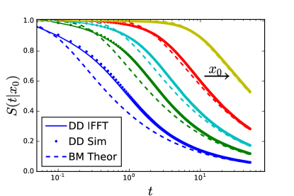
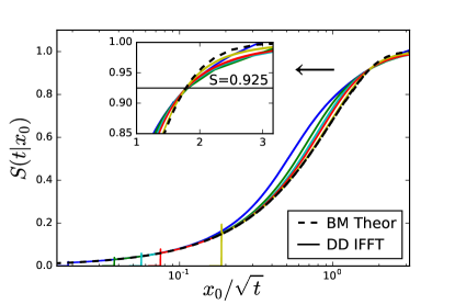
Figure 1: Left: Comparison of numerical and analytical results for the survival probability $S(t|x_{0})$ in the semi-infinite interval. Different colours represent the initial positions $x_{0}=0.5$, $1$, $1.5$, $2$, and $5$. Dashed lines in both panels represent the results of the corresponding Brownian-Gaussian motion. The numerical results (dots) obtained through Monte Carlo simulations are in full agreement with the analytical trend (solid line) obtained from numerical integration of the inverse Fourier transform (11). Right: analytical results for the survival probability in rescaled units in the semi-infinite domain as function of $x_{0}/\sqrt{t}$. In the inset the short time behaviour of $S(t|x_{0})$ is reported, the universal crossover at $S\approx 0.925$ is distinct.

Figure 1 (right) demonstrates two universalities. First, we observe that at intermediate times the survival probabilities for any initial position show a universal convergence to a common crossover point at around $S(t|x_{0})\approx 0.925$, including the Brownian-Gaussian survival probability. At times shorter than this crossover point Brownian-Gaussian motion is outperformed by the DD model, which assumes smaller values of $S(t|x_{0})$. At times longer than the crossover time the decay of Brownian-Gaussian motion is the fastest. Second, the initial advantage of the DD first passage dynamics over Brownian-Gaussian motion which reverts after the universal crossover point, appears to balance out: at long times the survival probability in all cases converges to the exact result of Brownian-Gaussian motion with effective diffusivity $\langle D\rangle_{\mathrm{st}}$. This can be seen directly from result (16), the associated first passage density of which is exactly the well-known Lévy-Smirnov form $\wp(t)=(x_{0}/\sqrt{4\pi\langle D\rangle_{\mathrm{st}}t^{3}})\exp(-x_{0}^{2}/[4\langle D\rangle_{\mathrm{st}}t]$).

Qualitatively a similar behaviour is observed for finite domains at short times. As shown in figure 2, in contrast, the long time behaviour is dominated by the exponential shoulder (20) corresponding to the lowest non-zero eigenvalue in the DD model. The corresponding characteristic time scale $\tau$ in figure 2 is longer than for Brownian-Gaussian motion. This is due to the fact that in the finite interval the particles will reach the boundary before experiencing the entire diffusivity space, and so the effective Brownian limit is not recovered. The larger the interval $L$ is the smaller the difference between the characteristic times of DD and Brownian-Gaussian models will be. In the limit of $L\to\infty$ the same long time behaviour is observed. Figure 2 also demonstrates an interesting behaviour of the superstatistical model. When the diffusivity distribution (2) governs the particle motion at all times $t$, even in the finite domain a power law scaling of the survival probability emerges, and thus a diverging mean first passage time is produced. This behaviour is caused by appreciable fraction of immobile particles manifested in the divergence or nonzero value of $p_{D}(D=0)$ in $d=1$ and $d=2$, respectively. This behaviour is rectified in the DD model.

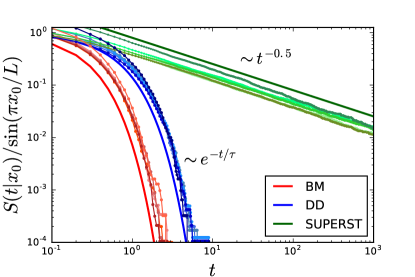
Figure 2: Survival probability for the finite interval $[0,L]$, showing a comparison between Brownian-Gaussian diffusion, DD, and superstatistical dynamics. Different colour shades represent different initial positions $x_{0}$, and the solid lines represent the analytical trends. The normalisation is chosen considering that all 3 models present the dependence on the initial position through the sinusoidal function reported in the $y$-axis and that at long times just the first eigenstate dominates. Indeed we observe that at long times all lines approach a quasi-master curve which is different for each model and in agreement with the analytical results: a power law asymptotic for the superstatistical model and exponential tails for the DD and Brownian-Gaussian models, the latter with two different $\tau$ values of the dominant exponential tail.

5 Conclusions

We studied the first passage behaviour of the popular DD model used as a mean field proxy for diffusion of test particles in heterogeneous environments, in which the particle experiences varying diffusivities. Our analysis demonstrated that at short times the DD dynamics leads to a faster decay of the survival probability and thus to more efficient first passage. In a semi-infinite domain, fully independent of the initial particle position a universal crossover occurs, beyond which the DD dynamics becomes less efficient than pure Brownian-Gaussian motion, and the ultimate decay is determined by the conventional Lévy-Smirnov behaviour for initial particle position $x_{0}$ and effective diffusivity $\langle D\rangle_{\mathrm{st}}$. The initial advantage of the DD dynamics may be particularly relevant in cases of molecular regulation processes at very low concentrations (few-encounter limit) [31]. At long times in finite domains the DD first passage behaviour is dominated by an exponential shoulder with a characteristic time (approximately the mean first passage time) that is longer than that for Brownian-Gaussian motion.

These results are in agreement with the expectation that rare events, represented by the exponential tails of the particles displacement distribution at short times, may dominate triggered actions. Thus, even if in general heterogeneity in the environment does not improve the mean first passage result (in fact some of the particles are slowed down) it allows some other particles to have a diffusion coefficient greater than the average, and this is enough to increase the efficiency of the reaction activation. Moreover, we proved that the amount of fast particles is independent on the initial position, representing the distance between particle and target. This suggests that the obtained results may be qualitatively generalised to any distribution of the initial particle position.

The study developed here is not limited to the one-dimensional case. First of all, we know that in the semi-infinite domain the results of the survival probability of Brownian-Gaussian motion in $d=2$ and $d=3$ are the same as the one in $d=1$. Then, the same analysis of the first passage problem can be performed by solely changing to the corresponding $d$-dimensional subordinator. For finite domains the analysis is also similar since, for all $d$ we have an exponential behaviour in time of the propagator which allows us to relate the DD survival probability to the Laplace transform of the corresponding subordinator, as we did for the one-dimensional case.

We finally note that similar non-Gaussian effects have been reported for systems, in which the (subdiffusive) motion is dominated by viscoelastic effects. With a fixed diffusivity this would be a Gaussian process, and the non-Gaussianity was shown to stem from varying diffusivity values [32, 33, 34]. It will be interesting to study the associated first passage behaviour in this case, as well.

References

References

- [1] Brown R 1828 A Brief Account of Microscopical Observations Made on the Particles Contained in the Pollen of Plants Phil. Mag. 4 161.
- [2] van Kampen N G 1981 Stochastic Processes in Physics and Chemistry (North Holland Publishing Company, Amsterdam).
- [3] Höfling F & Franosch T 2013 Anomalous transport in the crowded world of biological cells Rep. Prog. Phys. 76 046602.
- [4] Nørregaard K, Metzler R, Ritter C, Berg-Sørensen K & Oddershede L 2017 Manipulation and motion of organelles and single molecules in living cells, Chem. Rev. 117, 4342.
- [5] Bouchaud JP & Georges A 1990 Anomalous diffusion in disordered media: statistical mechanisms, models and physical applications Phys. Rep. 195, 127-293.
- [6] Metzler R, Jeon JH, Cherstvy AG & Barkai E 2014 Anomalous Diffusion Models and Their Properties: Non-stationarity, Non-ergodicity and Ageing at the Centenary of Single Particle Tracking Phys.Chem. Chem. Phys. 16 24128-24164.
- [7] Mandelbrot B B & van Ness J W 1968, Fractional Brownian motions, fractional noises and applications SIAM Review 10 422–437.
- [8] Scher H & Montroll E W 1975 Anomalous transit-time dispersion in amorphous solids Phys. Rev. B 12 2455.
- [9] Cherstvy A G, Chechkin A V & Metzler R 2013 Anomalous diffusion and ergodicity breaking in heterogeneous diffusion processes New J. Phys. 15 083039.
- [10] Wang B, Kuo J, Bae S C & Granick S 2012 When Brownian Diffusion Is Not Gaussian Nat. Mater. 11 481–485.
- [11] Wang B, Antony S M, Bae S C & Granick S 2009 Anomalous Yet Brownian Proc. Nat. Acad, Sci. U.S.A. 106 15160–15164.
- [12] Leptos K C, Guasto J S, Gollub J P, Pesci A I & Goldstein R E 2009 Dynamics of Enhanced Tracer Diffusion in Suspensions of Swimming Eukaryotic Microorganisms Phys. Rev. Lett. 103 198103.
- [13] Hapca S, Crawford JW & Young IM 2009 Anomalous diffusion of heterogeneous populations characterized by normal diffusion at the individual level J. Roy. Soc. Interface 6, 111-122.
- [14] Cherstvy AG, Nagel O, Beta C & Metzler R 2018 Non-Gaussianity, population heterogeneity, and transient superdiffusion in the spreading dynamics of amoeboid cells Phys. Chem. Chem. Phys. 20, 23034
- [15] Beck C & Cohen EDB 2003 Superstatistics Physica A 322, 267.
- [16] Beck C 2006 Superstatistical Brownian Motion Prog. Theor. Phys. Suppl. 162 29–36.
- [17] Chubynsky M V & Slater G W 2014 Diffusing Diffusivities: A Model for Anomalous, Yet Brownian Diffusion Phys. Rev. Lett. 113 098302.
- [18] Matse M, Chubynsky M V & Bechhoefer J 2017 Test of the diffusing-diffusivity mechanism using nearwall colloidal dynamics arXiv:1706.02039v1
- [19] Jain R & Sebastian K L 2016 Diffusion in a Crowded, Rearranging Environment J. Phys. Chem. B 120 3988–92.
- [20] Jain R & Sebastian K L 2017 Diffusing diffusivity: a new derivation and comparison with simulations J. Chem. Sci. 129 929–937.
- [21] Tyagi N & Cherayil B J 2017 Non-Gaussian Brownian Diffusion in Dynamically Disordered Thermal Environments J. Phys. Chem. B, 121 7204–7209.
- [22] Chechkin A V, Seno F, Metzler R & Sokolov I 2017 Brownian Yet Non-Gaussian Diffusion: From Superstatistics to Subordination of Diffusing Diffusivities Phys. Rev. X 7 021002.
- [23] Sposini V, Chechkin A V, Seno F, Pagnini G & Metzler R 2018 Random diffusivity from stochastic equations: comparison of two models for Brownian yet non-Gaussian diffusion New J. Phys., 20 043044.
- [24] Lanoiselée Y & Grebenkov D 2018 A model of non-Gaussian diffusion in heterogeneous media J. Phys. A, 51 145602.
- [25] Redner S 2001 A Guide to First Passage Processes (Cambridge, Cambridge University Press).
- [26] Metzler R, Oshanin G & Redner S 2014 First-Passage Phenomena and Their Applications (Singapore, World Scientific).
- [27] Bochner S 1960 Harmonic analysis and the theory of probability (Berkeley University Press)
- [28] Mura A & Pagnini G 2008 Characterizations and simulations of a class of stochastic processes to model anomalous diffusion J. Phys. A: Math. Theor. 41 285003.
- [29] Sliusarenko O, Vitali S, Sposini V, Paradisi P, Chechkin AV, Castellani G & Pagnini G 2018 Finite-energy Lévy-type motion through heterogeneous ensemble of Brownian particles arXiv:1807.07883 [cond-mat.stat-mech].
- [30] Prudnikov A P 1986 Integrals and series. Volume 2: special functions (CRC Press).
-
[31]
Godec A & Metzler R 2016 Universal proximity effect in target search
kinetics in the few encounter limit, Phys. Rev. X 6, 041037.
Godec A & Metzler R 2017 First passage time statistics for two-channel diffusion, J. Phys. A 50, 084001. - [32] Jeon J-H, Javanainen M, Martinez-Seara H, Metzler R & Vattulainen I 2016 Protein crowding in lipid bilayers gives rise to non-Gaussian anomalous lateral diffusion of phospholipids and proteins Phys. Rev. X 6, 021006.
-
[33]
Lampo T, Stylianido S, Backlund M P, Wiggins P A & Spakowitz
A J 2017 Cytoplasmic RNA-Protein Particles Exhibit Non-Gaussian Subdiffusive behaviour
Biophys. J. 112 532–542.
Metzler R 2017 Gaussianity Fair:The Riddle of Anomalous yet Non-Gaussian Diffusion Biophys. J. - New and Notable 112 413–415. - [34] He W, Song H, Su Y, Geng L, Ackerson BJ, Peng HB & Tong P 2016 Dynamic heterogeneity and non-Gaussian statistics for acetylcholine receptors on live cell membranes Nat. Comm. 7, 11701.