The $R$-Process Alliance: First Release from the Northern Search for $r$-Process Enhanced Metal-Poor Stars in the Galactic Halo

Abstract

This paper presents the detailed abundances and $r$-process classifications of 126 newly identified metal-poor stars as part of an ongoing collaboration, the $R$-Process Alliance. The stars were identified as metal-poor candidates from the RAdial Velocity Experiment (RAVE) and were followed-up at high spectral resolution ($R~{}\sim~{}31,500$) with the 3.5 m telescope at Apache Point Observatory. The atmospheric parameters were determined spectroscopically from Fe I lines, taking into account $<$3D$>$ non-LTE corrections and using differential abundances with respect to a set of standards. Of the 126 new stars, 124 have $[\rm{Fe/H}]<-1.5$, 105 have $[\rm{Fe/H}]<-2.0$, and 4 have $[\rm{Fe/H}]<-3.0$. Nine new carbon-enhanced metal-poor stars have been discovered, 3 of which are enhanced in $r$-process elements. Abundances of neutron-capture elements reveal 60 new $r$-I stars (with $+0.3~{}\leq~{}[\rm{Eu/Fe}]~{}\leq~{}+1.0$ and $[\rm{Ba/Eu}]<0$) and 4 new $r$-II stars (with $[\rm{Eu/Fe}]>+1.0$). Nineteen stars are found to exhibit a “limited-$r$” signature ($[\rm{Sr/Ba}]>+0.5$, $[\rm{Ba/Eu}]<0$). For the $r$-II stars, the second- and third-peak main $r$-process patterns are consistent with the $r$-process signature in other metal-poor stars and the Sun. The abundances of the light, $\alpha$, and Fe-peak elements match those of typical Milky Way halo stars, except for one $r$-I star which has high Na and low Mg, characteristic of globular cluster stars. Parallaxes and proper motions from the second Gaia data release yield $UVW$ space velocities for these stars which are consistent with membership in the Milky Way halo. Intriguingly, all $r$-II and the majority of $r$-I stars have retrograde orbits, which may indicate an accretion origin.

1 Introduction

Metal-poor stars ($[\rm{Fe/H}]\lesssim-1.0$) have received significant attention in recent years, primarily because they are believed to be some of the oldest remaining stars in the Galaxy (Beers & Christlieb, 2005; Frebel & Norris, 2015). High-precision abundances of a wide variety of elements, from lithium to uranium, provide valuable information about the early conditions in the Milky Way (MW), particularly the nucleosynthesis of rare elements, yields from early neutron star mergers (NSMs) and supernovae, and the chemical evolution of the MW. The low iron content of the most metal-poor stars suggests that their natal gas clouds were polluted by very few stars, in some cases by only a single star (e.g., Ito et al. 2009; Placco et al. 2014a). Observations of the most metal-poor stars therefore provide valuable clues to the formation, nucleosynthetic yields, and evolutionary fates of the first stars and the early assembly history of the MW and its neighboring galaxies.

The stars that are enhanced in elements that form via the rapid ($r$-) neutron-capture process are particularly useful for investigating the nature of the first stars and early galaxy assembly (e.g., Sneden et al. 1996; Hill et al. 2002; Christlieb et al. 2004; Frebel et al. 2007; Roederer et al. 2014b; Placco et al. 2017; Hansen et al. 2018; Holmbeck et al. 2018a). The primary nucleosynthetic site of the $r$-process is still under consideration. Photometric and spectroscopic follow-up of GW 170817 (Abbott et al., 2017) detected signatures of $r$-process nucleosynthesis (e.g., Chornock et al. 2017; Drout et al. 2017; Shappee et al. 2017), strongly supporting the NSM paradigm (e.g., Lattimer & Schramm 1974; Rosswog et al. 2014; Lippuner et al. 2017). This paradigm is also supported by chemical evolution arguments (e.g., Cescutti et al. 2015; Côté et al. 2017), comparisons with other abundances (e.g., Mg; Macias & Ramirez-Ruiz 2016), and detections of $r$-process enrichment in the ultra faint dwarf galaxy Reticulum II (Ji et al., 2016; Roederer et al., 2016; Beniamini et al., 2018).

However, the ubiquity of the $r$-process (Roederer et al., 2010), particularly in a variety of ultra faint dwarf galaxies, suggests that NSMs may not be the only site of the $r$-process (Tsujimoto & Nishimura, 2015; Tsujimoto et al., 2017). Standard core-collapse supernovae are unlikely to create the main $r$-process elements (Arcones & Thielemann , 2013); instead, the most likely candidate for a second site of $r$-process formation may be the “jet supernovae,” the resulting core collapse supernovae from strongly magnetic stars (e.g., Winteler et al. 2012; Cescutti et al. 2015). The physical conditions (electron fraction, temperature, density), occurrence rates, and timescales for jet supernovae may differ from NSMs—naively, this could lead to different abundance patterns (particularly between the $r$-process peaks) and different levels of enrichment (e.g., see Mösta et al. 2017). This then raises several questions. Why is the relative abundance pattern for the main $r$-process (barium and above) so robust across $\sim 3$ dex in metallicity (e.g., Sakari et al. 2018)? (In other words, why don’t the $r$-process yields vary?) Why is $r$-process contamination so ubiquitous, even in low-mass systems where $r$-process events should be rare? Finally, how can such low-mass systems like the ultra faint dwarf galaxies retain the ejecta from such energetic events? (See Bland-Hawthorn et al. 2015 and Beniamini et al. 2018 for discussions of the mass limits of dwarfs that can retain ejecta for subsequent star formation.) Addressing these questions requires collaboration between theorists, experimentalists, modelers, and observers.

Observationally, the $r$-process-enhanced, metal-poor stars may provide the most useful information for identifying the site(s) of the $r$-process. There are two main reasons for this: 1) The enhancement in $r$-process elements ensures that spectral lines from a wide variety of $r$-process elements are sufficiently strong to be measured, while the (relative) lack of metal lines (compared to more metal-rich stars) reduces the severe blending typically seen in the blue spectral region; and 2) These stars are selected to have little-to-no contamination from the slow ($s$-) process, simplifying comparisons with models of $r$-process yields. If the enhancement in radioactive elements like Th and U is sufficiently high, cosmo-chronometric ages can also be determined (see, e.g., Holmbeck et al. 2018a and references therein).

The $r$-process-enhanced, metal-poor stars have historically been divided into two main categories (Beers & Christlieb, 2005): the $r$-I stars have $+0.3\leq[\rm{Eu/Fe}]\leq+1.0$, while $r$-II stars have $[\rm{Eu/Fe}]~{}>~{}+1.0$; both require $[\rm{Ba/Eu}]<0$ to avoid contamination from the $s$-process. Prior to 2015, there were $\sim 30$ $r$-II and $\sim 75$ $r$-I stars known, according to the JINAbase compilation (Abohalima et al., 2017). Observations of these $r$-process-enhanced stars have found a common pattern among the main $r$-process elements, which is in agreement with the Solar $r$-process residual. Despite the consistency of the main $r$-process patterns, $r$-process-enhanced stars are known to have deviations from the Solar pattern for the lightest and heaviest neutron-capture elements. Variations in the lighter neutron-capture elements, such as Sr, Y, and Zr have been observed in several stars (e.g., Siqueira Mello et al. 2014; Placco et al. 2017; Spite et al. 2018). A new limited-$r$ designation (Frebel, 2018), with $[\rm{Sr/Ba}]~{}>~{}+0.5$, has been created to classify stars with enhancements in these lighter elements. (Though note that fast rotating massive stars can create some light elements via the $s$-process; Chiappini et al. 2011; Frischknecht et al. 2012; Cescutti et al. 2013; Frischknecht et al. 2016. In highly $r$-process-enhanced stars, however, this signal may be swamped by the larger contribution from the $r$-process; Spite et al. 2018.) A subset of $r$-II stars ($\sim 30$%) also exhibit an enhancement in Th and U that is referred to as an “actinide boost” (e.g., Hill et al. 2002; Mashonkina et al. 2014; Holmbeck et al. 2018a)—a complete explanation for this phenomenon remains elusive (though Holmbeck et al. 2018b propose one possible model), but it may prove critical for constraining the $r$-process site(s).

The numbers of stars in these categories will be important for understanding the source(s) of the $r$-process. If NSMs are the dominant site of the $r$-process, they may be responsible for the enhancement in both $r$-I and $r$-II stars—if so, the relative frequencies of $r$-I and $r$-II stars can be compared with NSM rates. Finally, there has been speculation that $r$-process-enhanced stars may form in dwarf galaxies (e.g., Reticulum II; Ji et al. 2016), which are later accreted into the MW. The combination of abundance information from high-resolution spectroscopy and proper motions and parallaxes from Gaia DR2 (Gaia Collaboration et al., 2018) will enable the birth sites of the $r$-process-enhanced stars to be assessed, as has already been done for several halo $r$-II stars (Sakari et al., 2018; Roederer et al., 2018a).

These are the observational goals of the $R$-Process Alliance (RPA), a collaboration with the aim of identifying the site(s) of the $r$-process. This paper presents the first data set from the Northern Hemisphere component of the RPA’s search for $r$-process-enhanced stars in the MW; the first Southern Hemisphere data set is presented in Hansen et al. (2018). The observations and data reduction for this sample are outlined in Section 2. Section 3 presents the atmospheric parameters (temperature, surface gravity, and microturbulence) and Fe and C abundances of a set of standard stars, utilizing Local Thermodynamic Equilibrium (LTE) Fe I abundances both with and without non-LTE (NLTE) corrections. The parameters for the targets are then determined differentially with respect to the set of standards. The detailed abundances are given in Section 4; Section 5 then discusses the $r$-process classifications, the derived $r$-process patterns, implications for the site(s) of the $r$-process, and comparisons with other MW halo stars. The choice of NLTE corrections is justified by comparisons with other techniques for deriving atmospheric parameters, e.g., photometric temperatures, in Appendix A. LTE parameters and abundances are also provided in Appendix B, and a detailed analysis of systematic errors is given in Appendix C. Future papers from the RPA will present additional discoveries of $r$-I and $r$-II stars.

2 Observations and Data Reduction

The metal-poor targets in this study were selected from two sources. Roughly half of the stars were selected from the fourth (Kordopatis et al., 2013a) and fifth (Kunder et al., 2017) data releases from the RAdial Velocity Experiment (Steinmetz et al., 2006, RAVE) and the Schlaufman & Casey (2014) sample. These stars had their atmospheric parameters ($T_{\rm{eff}}$, $\log g$, and [Fe/H]) and [C/Fe] ratios validated through optical ($3500-5500$ Å), medium-resolution ($R~{}\sim~{}2000$) spectroscopy (Placco et al., 2018). The other half were part of a re-analysis of RAVE data by Matijevic̆ et al. (2017). The stars that were targeted for high-resolution follow-up all had metallicity estimates $[\rm{Fe/H}]\lesssim-1.8$ and (in the case of the Placco et al. subsample) were not carbon enhanced. Additionally, twenty previously observed metal-poor stars were included to serve as standard stars. Altogether, 131 stars with $V$-band magnitudes between 9 and 13 were observed, as shown in Table 1, where IDs, coordinates, and magnitudes are listed.

All targets were observed in 2015-2017 with the Astrophysical Research Consortium (ARC) 3.5 - m telescope at Apache Point Observatory (APO). The seeing ranged from $0.6-2\arcsec$, with a median value of $1.15\arcsec$. The ARC Echelle Spectrograph (ARCES) was utilized in its default setting, with a $1.6\arcsec\times 3.2\arcsec$ slit, providing a spectral resolution of $R\sim 31,500$. The spectra cover the entire optical range, from $3800-10400$ Å, though the S/N is often prohibitively low below 4000 Å. Initial “snapshot” spectra were taken to determine $r$-process enhancement; exposure times were typically adjusted to obtain S/N ratios $>30$ (per pixel) in the blue, which leads to S/N ratios $\gtrsim 60$ near 6500 Å. Any interesting targets were then observed again to obtain higher S/N. Observation dates, exposure times, and S/N ratios are reported in Table 1.

The data were reduced in the Image Reduction and Analysis Facility program (IRAF) with the standard ARCES reduction recipe (see the manual by J. Thorburn), yielding non-normalized spectra with 107 orders each. The blaze function was determined empirically through Legendre polynomial fits to high S/N, extremely metal-poor stars. The spectra of the other targets were divided by these blaze function fits and refit with low-order (5-7) polynomials (with strong lines, molecular bands, and telluric features masked out). All spectra were shifted to the rest-frame through cross-correlations with a very high-resolution, high S/N spectrum of Arcturus (from the Hinkle et al. 2003 atlas). The individual observations were then combined with average $\sigma$-clipping techniques, weighting the individual spectra by their flux near 4150 Å. Sample spectra around the 4205 Å  Eu II line are shown in Figure 1.

The final S/N ratios and heliocentric radial velocities are given in Tables 1, while Figure 2 shows a comparison with the radial velocities from RAVE and Gaia DR2 (Gaia Collaboration et al., 2016, 2018). The agreement is generally excellent, with a small median offset and standard deviation of $-1.1\pm 3.2$ km s^-1 from RAVE and $-0.8\pm 2.9$ km s^-1 from Gaia. There are several outliers with offsets $1\sigma$ from the mean, which may be binaries. In the case of J0145$-$2800, J0307$-$0534, and J0958$-$1446, multi-epoch observations in this paper show large radial velocity variations; in these cases, the RAVE and Gaia radial velocities also differ. Even if these stars are unresolved binaries, none of the spectra show any signs of contamination from a companion.

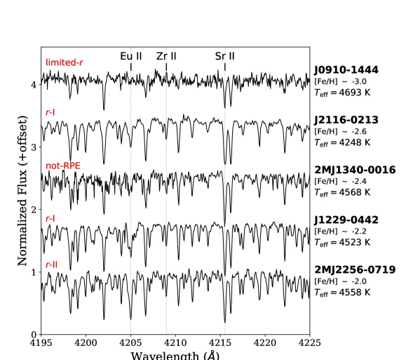
Figure 1: Sample spectra for stars with a range of S/N, metallicity, temperature, and $r$-process enhancement. “Not-RPE” indicates that the stars is not enhanced in $r$-process elements. Three Sr II, Zr II, and Eu II lines that were used in this analysis are identified.

Table 1: Targets

Star	RA	Dec	$V$	Observation	Exposure	S/N		$v_{\rm{helio}}$		Note
	(J2000)			Dates	Time (s)	4400 Å	6500 Å	(km s-1)
J000738.2$-$034551	00:07:38.16	$-$03:45:50.4	11.52	9, 11 Sep 2016	2700	60	156	-145.9±1	P18
J001236.5$-$181631	00:12:36.47	$-$18:16:31.0	10.95	22 Jan, 28 Sep 2016	1500	80	150	-96.4±0
J002244.9$-$172429	00:22:44.86	$-$17:24:29.1	12.89	22 Jan, 28 Sep 2016	3600	18	62	91.8±1
J003052.7$-$100704	00:30:52.67	$-$10:07:04.2	12.77	28 Sep 2016,	2700	25	60	-88.4±3
				2 Feb 2017
J005327.8$-$025317	00:53:27.84	$-$02:53:16.8	10.34	20 Jan 2016	2400	53	220	-197.7±0	P18
				31 Jan 2017
J005419.7$-$061155	00:54:19.65	$-$06:11:55.4	13.06	28 Sep 2016	1800	20	75	-132.8±0
J010727.4$-$052401	01:07:27.37	$-$05:24:00.9	11.88	28 Sep 2016	1800	58	98	-1.4±0
J012042.2$-$262205	01:20:42.20	$-$26:22:04.7	10.21	22 Jan 2016	1200	43	100	15.2±0
CS 31082-0001	01:29:31.14	$-$16:00:45.5	11.32	22 Jan 2016	1440	30	106	137.6±0	Std
J014519.5$-$280058	01:45:19.52	$-$28:00:58.4	11.55	2 Feb, 28 Dec 2017	3000	20	75	36.9±3

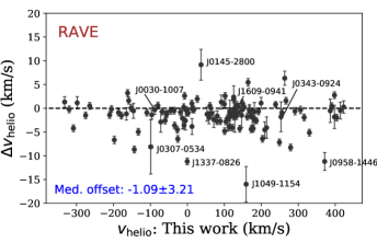
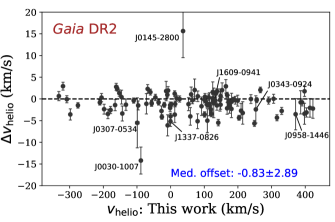
Figure 2: A comparison of the average heliocentric radial velocities in this work with those from RAVE (left) and Gaia DR2 (right). There are 122 stars with RAVE velocities, and 111 with Gaia DR2 velocities. The labeled outliers have offsets $>1\sigma$ from the median and/or large dispersions in velocity, and may be binaries.

3 Atmospheric Parameters, Metallicities, and Carbon Abundances

High-resolution analyses utilize a variety of techniques to refine the stellar temperatures, surface gravities, microturbulent velocities, and metallicities, each with varying strengths and weaknesses. The most common way to determine atmospheric parameters is from the strengths of Fe lines, under assumptions of LTE. Note that the atmospheric parameters are all somewhat degenerate—the assumption of LTE therefore can systematically affect all the parameters. In a typical high-resolution analysis, temperatures and microturbulent velocities are found by removing any trends in the Fe I abundance with line excitation potential (EP) and reduced EW (REW), respectively. However, each Fe I line will have a different sensitivity to NLTE effects. Similarly, surface gravities are sometimes determined by requiring agreement between the Fe I and Fe II abundances; however, the abundances derived from Fe I lines more sensitive to NLTE effects than those from Fe II lines (Kraft & Ivans, 2003). There are ways to determine the stellar parameters that will not be as affected by NLTE effects, e.g., using colors (Ramírez & Meléndez, 2005; Casagrande et al., 2010) to determine temperatures or isochrones to determine surface gravities (e.g., Sakari et al. 2017), but these techniques require some a priori knowledge of the reddening, distance, etc. Some groups also utilize empirical corrections to LTE spectroscopic temperatures to more closely match the photometric temperatures (e.g., Frebel et al. 2013). Recently, it has become possible to apply NLTE corrections directly to the LTE abundances (Lind et al., 2012; Ruchti et al., 2013; Amarsi et al. , 2016; Ezzeddine et al., 2017). This technique has the benefit of enabling the atmospheric parameters to be determined solely from the spectra.

An ideal approach should provide the most accurate abundances for future use, while maintaining compatibility with other samples of metal-poor stars. Sections 3.1 and Appendix A demonstrate that adopting spatially- and temporally-averaged three-dimensional ($<$3D$>$), NLTE corrections (in this case from Amarsi et al. 2016) provide parameters that are in better agreement with independent methods, compared to purely spectroscopic LTE parameters. Although NLTE-corrected parameters from $<$3D$>$ models are ultimately selected as the preferred values in this paper, LTE parameters and abundances are provided in Appendix B to facilitate comparisons with LTE studies. Section 3.2 presents the adopted parameters for the target stars, Section 3.3 discusses the [C/Fe] ratios, and Section 3.4 then discusses the uncertainties in these parameters.

In the analyses that follow, Fe abundances are determined from equivalent widths (EWs), which are measured using the program DAOSPEC (Stetson & Pancino, 2008). Only lines with $\rm{REW}<-4.7$ were used, to avoid uncertainties that arise from, e.g., uncertain damping constants (McWilliam et al., 1995). All abundances are determined with the 2017 version of MOOG (Sneden, 1973), including an appropriate treatment for scattering (Sobeck et al., 2011). Kurucz model atmospheres were used (Castelli & Kurucz, 2004). For all cases below, the final atmospheric parameters are determined entirely from the spectra. Surface gravities are determined by enforcing ionization equilibrium in iron (i.e., the surface gravities are adjusted so that the average Fe I abundance is equal to the average Fe II abundance). Temperatures and microturbulent velocities are determined by flattening trends in Fe I line abundances with EP and REW. For the NLTE cases, corrrections were applied to LTE abundance from each Fe I line, according to the current atmospheric parameters in that iteration. The corrections are determined with the interpolation grid from Amarsi et al. (2016).

3.1 Standard Stars

The parameters of the previously observed standard stars are first presented, to 1) establish the effects of the NLTE corrections on the atmospheric parameters and 2) demonstrate agreement with results from the literature.

3.1.1 LTE vs. NLTE

The LTE and NLTE atmospheric parameters for the standard stars are shown in Table 2. The naming convention of Amarsi et al. (2016) is adopted: the 1D, NLTE corrections are labeled “NMARCS” while the $<$3D$>$, NLTE corrections are “NMTD” (i.e., NMARCS 3D). These corrections were applied as in Ruchti et al. (2013), using the 1D and $<$3D$>$ NLTE grids from Amarsi et al. (2016). The interpolation scheme from Lind et al. (2012) and Amarsi et al. (2016) is used to determine the appropriate corrections for each set of atmospheric parameters; these corrections are then applied on-the-fly to the LTE abundance from each Fe I line (note that the NLTE corrections for the Fe II lines are negligible; Ruchti et al. 2013).

A qualitative trend is evident from Table 2, and is demonstrated in Figure 3. Compared to the LTE values, the NMARCS corrections moderately affect $T_{\rm{eff}}$, while the NMTD corrections increase $T_{\rm{eff}}$. The surface gravities and metallicities are also generally increased when the NLTE corrections are applied, while the microturbulent velocities decrease. These changes are most severe at the metal-poor end and for the cooler giants. It is worth noting that these changes qualitatively agree with the known problems that occur in purely spectroscopic LTE analyses, where the temperatures, surface gravities, and metallicities that are derived from Fe I lines are known to be under-estimated, while the microturbulent velocities are over-estimated. Appendix A more completely validates the choice of the NMTD parameters through comparisons with photometric temperatures and parallax-based distances.

Table 2: Atmospheric Parameters and [C/Fe]: Standard Stars

	LTE				NMARCS				NMTD
	$T_{\rm{eff}}$	$\log g$	$\xi\;\;\;\;$	[Fe/H]	$T_{\rm{eff}}$	$\log g$	$\xi\;\;\;\;$	[Fe/H]	$T_{\rm{eff}}$	$\log g$	$\xi\;\;\;\;$	[Fe I/H] ($N$)		[C/Fe]
Star	(K)	(km s-1)			(K)	(km s-1)			(K)	(km s-1)
CS 31082-001	4827	1.65	1.70	$-2.79$	4827	1.95	1.59	$-2.68$	4877	1.95	1.44	-2.64±0	0.04±0.10
TYC 5861-1732-1	4850	1.77	1.34	$-2.47$	4825	1.87	1.23	$-2.39$	4925	2.07	1.16	-2.29±0	-0.29±0.11
CS 22169-035	4483	0.50	2.01	$-3.03$	4458	0.50	2.03	$-3.02$	4683	0.70	1.75	-2.80±0	0.58±0.10
TYC 75-1185-1	4793	1.34	1.72	$-2.88$	4793	1.54	1.63	$-2.79$	4943	1.94	1.53	-2.63±0	0.05±0.10
TYC 5911-452-1	6220	4.07	1.77	$-2.32$	6195	4.27	1.60	$-2.19$	6295	4.47	1.50	-2.08±0	-0.15±0.20
TYC 5329-1927-1	4393	0.30	2.14	$-2.41$	4368	0.20	2.12	$-2.41$	4568	0.90	2.01	-2.28±0	0.43±0.11
TYC 6535-3183-1	4320	0.46	1.92	$-2.12$	4295	0.36	1.91	$-2.15$	4370	0.56	1.89	-2.09±0	0.23±0.10
TYC 4924-33-1	4831	1.72	1.69	$-2.36$	4806	1.82	1.62	$-2.30$	4831	1.72	1.54	-2.28±0	0.27±0.10
HE 1116$-$0634	4248	0.01	2.17	$-3.72$	4198	0.01	2.28	$-3.75$	4698	1.11	1.65	-3.28±0	0.54±0.20
TYC 6088-1943-1	4931	1.95	1.57	$-2.54$	4931	2.25	1.50	$-2.43$	4956	2.25	1.34	-2.45±0	-0.14±0.11
BD-13 3442	6299	3.69	1.50	$-2.80$	6299	4.09	1.35	$-2.64$	6349	4.29	1.28	-2.56±0	¡0.55
BD-01 2582	4960	2.24	1.46	$-2.49$	4960	2.54	1.40	$-2.37$	4985	2.44	1.24	-2.33±0	0.71±0.10
HE 1317$-$0407	4660	0.76	1.87	$-2.89$	4660	0.86	1.79	$-2.83$	4835	1.16	1.69	-2.66±0	0.15±0.20
HE 1320$-$1339	4591	0.50	1.66	$-3.06$	4591	0.60	1.60	$-3.02$	4841	1.10	1.46	-2.76±0	0.0±0.20
HD 122563	4374	0.46	2.06	$-2.96$	4324	0.26	2.09	$-2.97$	4624	0.96	1.76	-2.71±0	0.49±0.13
TYC 4995-333-1	4807	1.16	1.83	$-2.02$	4707	0.96	1.75	$-2.07$	4707	0.96	1.71	-2.06±0	0.14±0.10
HE 1523-0901	4290	0.20	2.13	$-3.09$	4315	0.40	2.16	$-3.06$	4590	0.90	1.73	-2.81±0	0.39±0.15
TYC 6900-414-1	4798	1.50	1.24	$-2.45$	4823	1.80	1.17	$-2.35$	4898	2.00	1.10	-2.28±0	-0.04±0.10
J2038-0023	4579	0.84	2.03	$-2.89$	4579	0.94	1.97	$-2.84$	4704	0.94	1.77	-2.71±0	0.59±0.10
BD-02 5957	4217	0.06	2.05	$-3.22$	4192	0.06	2.10	$-3.23$	4567	0.96	1.57	-2.91±0	0.54±0.10

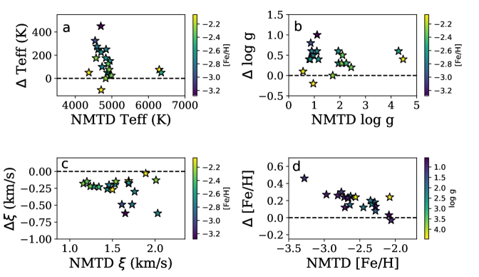
Figure 3: Offsets in the atmospheric parameters (NMTD $-$ LTE), as a function of the NMTD parameters, for the standard stars. In panels a, b, and c, the points are color-coded according to their [Fe/H] ratios, while in panel d they are color-coded according to surface gravities.

The NMARCS parameters were also compared with parameters derived using the 1D NLTE corrections following Ezzeddine et al. (2017). Similar to the process for the Amarsi et al. (2016) corrections, the NLTE corrections for each Fe I line were found by interpolating the measured EWs over a calculated grid of NLTE EWs over a dense parameter space in effective temperature, surface gravity, metallicity, and microturbulent velocity. The 1D MARCS model atmospheres (Gustafsson et al., 2008) were used with the NLTE radiative transfer code MULTI2.3 (Carlsson, 1986, 1992) to calculate the EW grid. A comprehensive Fe I/Fe II model atom is used in the calculations, with up-to-date inelastic collisions with hydrogen implemented from Barklem (2018); see Ezzeddine et al. (2016) for more details on the atomic model and data. Compared to the NMARCS values, the Ezzeddine et al. corrections lead to agreement in temperature within 50 K, surface gravities within 0.5 dex, microturbulent velocities within 0.5 km s^-1, and metallicities within 0.1 dex.

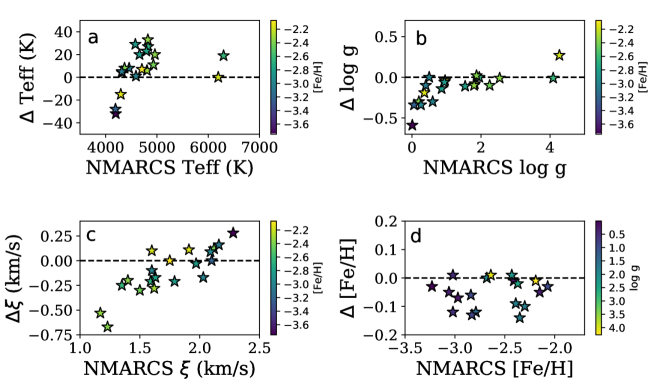
Figure 4: Offsets in the atmospheric parameters derived with 1D NLTE corrections (Amarsi et al. $-$ Ezzeddine et al.) for the standard stars. Panels are color-coded as in Figure 3.

3.1.2 Comparisons with Literature Values

The NMTD parameters are compared to LTE and NLTE literature values in Figure 5. As with any set of spectroscopic analyses, the techniques used to derive the atmospheric parameters vary significantly between groups; the points in Figure 5 are therefore grouped roughly by technique. Again, the results qualitatively make sense when compared with the LTE results from the literature (from Frebel et al. 2007; Hollek et al. 2011; Roederer et al. 2014a; Thanathibodee 2016; Placco et al. 2017): the NMTD temperatures are slightly higher than values derived spectroscopically, occasionally even when empirical corrections are included to raise the temperature. The surface gravities are typically higher than the values derived with LTE ionization equilibrium and isochrones, while the microturbulent velocities are much lower than the studies that utilize LTE ionization equilibrium to derive surface gravities. Finally, the [Fe/H] ratios agree reasonably well at the metal-rich end, but become increasingly discrepant with lower [Fe/H]. These findings are all consistent with those from Amarsi et al. (2016).

Hansen et al. (2013) and Ruchti et al. (2013) adopted NLTE corrections of some sort in previous analyses of standard stars in this paper, albeit with slightly different techniques for deriving the final atmospheric parameters. Hansen et al. (2013) adopted photometric temperatures and then applied 1D NLTE corrections to $\log g$ and [Fe/H]; the agreement with those points is generally good. Ruchti et al. (2013) applied 1D NLTE corrections to LTE abundances, as in this paper; a key difference, however, is that Ruchti et al. did not use Fe I lines with $\rm{EP}<2$ eV, which they argue are more sensitive to the NLTE effects. As a result, Ruchti et al. find even higher temperatures, surface gravities, and metallicities, values which would no longer agree with the previous LTE analyses, even when photometric temperatures and parallax-based surface gravities are adopted.

Given that the spectroscopic NMTD-corrected parameters in this paper agree well with the photometric temperatures and gravities from the literature (also see Appendix A), the NMTD parameters are adopted for the rest of the paper.

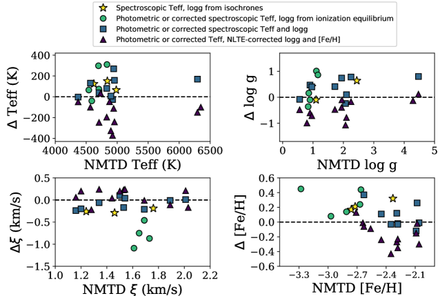
Figure 5: Differences between the $<$3D$>$, NLTE (NMTD) atmospheric parameters and parameters from the literature for the standard stars (NMTD$-$literature). Some stars are shown multiple times from different studies. The yellow stars show comparisons with spectroscopic LTE temperatures and isochrone-based surface gravities from Roederer et al. (2014a). The green circles show comparisons with Frebel et al. (2007), Hollek et al. (2011), Thanathibodee (2016), and Placco et al. (2017), LTE analyses that utilized either photometric temperatures or spectroscopic temperatures with corrections to match photometric temperatures, and surface gravities derived by requiring ionization equilibrium. The blue squares compare with Ruchti et al. (2011), who utilized photometric or corrected LTE spectroscopic temperatures and surface gravities derived from photometry. Finally, the purple triangles show comparisons with Hansen et al. (2013) and Ruchti et al. (2013), who used photometric or corrected spectroscopic temperatures and 1D NLTE corrections to determine the surface gravity and metallicity.

3.1.3 The Case of HD 122563

The standard HD 122563 was one of the stars in Amarsi et al. (2016), the paper which provides the $<$3D$>$, NLTE corrections that are used in this analysis. Amarsi et al. were able to achieve ionization equilibrium with NMTD corrections for all of their target stars except for HD 122563. They suggested that the parallax-based surface gravity from the literature was too high, and that $\log g\approx 1.1$ was more appropriate. Naturally, with the Amarsi et al. corrections the NMTD spectroscopic gravity in Table 2, $\log g=0.96$, is indeed lower than the parallax-based value used in Hansen et al. (2013). Roederer et al. (2014a) also find a lower value using isochrones. Indeed, Gaia DR2 provides a smaller parallax and error than the Hipparcos value: Gaia finds a parallax of $3.44\pm 0.06$, while Hipparcos found $4.22\pm 0.35$ (van Leeuwen, 2007). This suggests that the surface gravity is indeed lower (i.e., the star is farther away and intrinsically brighter) than previously predicted (also see Section A.2).

3.2 Atmospheric Parameters: Target Stars

Beyond the choice of LTE or NLTE, stellar abundance analyses suffer from a variety of other systematic errors as a result of, e.g., atomic data, choice of model atmospheres, etc. These effects have been mitigated in the past by performing differential analyses with respect to a set of standard stars. A differential analysis reduces the systematic offsets relative to the standard star, enabling higher precision parameters and abundances to be determined. This type of analysis has been performed on both metal-rich (Fulbright et al., 2006, 2007; Koch & McWilliam, 2008; McWilliam et al., 2013; Sakari et al., 2017) and metal-poor stars (O’Malley et al., 2017; Reggiani et al., 2016, 2017) and is the approach that is chosen for the target stars. The stars identified in Table 3 are used as the differential standards.

Each target is matched up with a standard star based on its initial atmospheric parameters, and $\Delta\log\epsilon$(Fe I) abundances are calculated for each line with respect to the standard, again using NLTE $<$3D$>$ corrections. Flattening the slopes in $\Delta\log\epsilon$(Fe I) with EP and REW provide the relative temperature and microturbulent velocity offsets for the target, while the offset between the $\Delta\log\epsilon$(Fe I) and $\Delta\log\epsilon$(Fe II) abundances is then used to determine the relative $\log g$. These relative offsets are then applied to the NLTE atmospheric parameters of the standard stars. If the atmospheric parameters are in better agreement with another standard, the more appropriate standard is selected and the process is redone. Note that the choice of standard does not significantly affect the final atmospheric parameters, unless the two stars have very different parameters (and therefore few lines in common); in this case, the final atmospheric parameters indicate that another standard would be more appropriate. This process is very similar to that of O’Malley et al. (2017), except that this analysis utilizes $<$3D$>$ NLTE corrections.

The final NMTD atmospheric parameters are shown in Table 3. Because LTE parameters are still widely used in the community, LTE parameters are also provided in Appendix B. However, it is worth noting that the NMTD values in this paper produce similar results to the photometric temperatures and gravities, and the LTE values may not be the best choice for comparisons with literature values.

The spectroscopic temperatures, gravities, and metallicities can be directly compared to stellar isochrones, e.g., the BaSTI/Teramo models (Pietrinferni et al., 2004). Figure 6 shows a spectroscopic HR-Diagram with the standard and target stars color-coded by [Fe/H]. Overplotted are 14 Gyr, $\alpha$-enhanced BaSTI isochrones at $[\rm{Fe/H}]=-1.84$, $-2.14$ and $-2.62$. The BaSTI isochrones persist through the AGB phase; extended AGBs with a mass-loss parameter of $\eta=-0.2$ are shown. Some of the brightest stars are slightly hotter than the RGB for their [Fe/H], indicating that they may be AGB stars. Four of the targets are main-sequence stars.

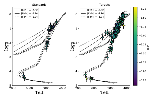
Figure 6: A Hertzsprung-Russell diagram showing surface gravity versus effective temperature. The standard stars are shown in the left panel, while the targets are shown in the right panel; both are color-coded by [Fe/H]. Three BaSTI isochrones are shown, with $[\rm{Fe/H}]=-1.84$, $-2.14$, and $-2.62$ (both with $[\alpha/\rm{Fe}]=+0.4$ and ages of 14 Gyr).

Table 3: Atmospheric Parameters and [C/Fe]: Target Stars

Star	Reference Standard	$T_{\rm{eff}}$ (K)	$\log g$	$\xi$ (km/s)	[Fe I/H] ($N$)		[Fe II/H] ($N$)	[C/Fe]
J0007$-$0345	TYC 5329-1927-1	4663	1.48	2.07	-2.09±0	-2.10±0.03  (24)	0.17±0
J0012$-$1816	BD$-$01 2582	4985	2.44	1.27	-2.28±0	-2.27±0.02  (17)	-0.26±0
J0022$-$1724	HE 1116-0634	4718	1.11	1.29	-3.38±0	-3.44±0.11  (3)	1.87±0
J0030$-$1007	TYC 4924-33-1	4831	1.48	1.97	-2.35±0	-2.34±0.06  (14)	0.50±0
J0053$-$0253	TYC 6535-3183-1	4370	0.56	1.81	-2.16±0	-2.16±0.04  (25)	0.40±0
J0054$-$0611	TYC 4995-333-1	4707	1.03	1.74	-2.32±0	-2.37±0.08  (15)	0.50±0
J0107$-$0524	BD$-$01 2582	5225	3.03	1.20	-2.32±0	-2.36±0.03  (13)	-0.09±0
J0145$-$2800	TYC 4995-333-1	4582	0.69	1.57	-2.60±0	-2.58±0.05  (12)	0.34±0
J0156$-$1402	TYC 4995-333-1	4622	1.09	2.27	-2.08±0	-2.07±0.05  (20)	0.37±0
2MJ0213$-$0005	TYC 5911-452-1	6225	4.54	2.33	-1.88±0	-1.93±0.08  (5)	-0.38±0

A small number of stars were also erroneously flagged as metal-poor ($[\rm{Fe/H}]<-1$) in the moderate-resolution observations. These stars are shown in Table 4, and include hot, metal-rich stars and cool M dwarfs.

Table 4: Stars that are Likely not Metal-Poor

	Type
J0120$-$2622	Hot, metal-rich star
J0958$-$0323	Hot, modestly metal-rich star ($[\rm{Fe/H}]\sim-0.8$)
J1555$-$0359	M star

3.3 Carbon

Carbon abundances were determined from syntheses of the CH $G$-band at 4312 Å  and the neighboring feature at 4323 Å. In some stars, particularly the hotter ones, only upper limits are available. The evolutionary corrections of Placco et al. (2014b) were applied to account for C depletion after the first dredge up. Most of the stars have [C/Fe] ratios that are consistent with typical metal-poor MW halo stars, though there are a few carbon-enhanced metal-poor (CEMP) stars with $[\rm{C/Fe}]~{}>~{}+~{}0.7$. One of the standards, BD$-$01 2582, is a CEMP star, in agreement with Roederer et al. (2014a). Of the targets, eight are found to be CEMP stars—these stars will be further classified according to their $r$- and $s$-process enrichment in Section 4.2.

3.4 Uncertainties in Atmospheric Parameters

Uncertainties in the atmospheric parameters are calculated for seven standard stars covering a range in [Fe/H], temperature, and surface gravity. The full details are given in Appendix C. Briefly, because the parameters are determined from Fe lines, the uncertainties increase with decreasing [Fe/H] and increasing temperature, a natural result of having fewer Fe I and Fe II lines. The detailed analysis in Appendix C demonstrates that the typical uncertainties in temperature range from 20 to 200 K, in $\log g$ from 0.05 to 0.3 dex, and in microturbulence from $0.10$ to $0.35$ km s^-1. These parameters are not independent, as demonstrated by the covariances in Table 10—however, the covariances are generally fairly small.

4 Chemical Abundances

All abundances are determined in MOOG. In general, lines with $\rm{REW}>-4.7$ are not utilized because of issues with damping and treatment of the outer layers of the atmosphere (McWilliam et al., 1995); some exceptions are made, and are noted below. The line lists were generated with the linemake code, and include hyperfine structure, isotopic splitting, and molecular lines from CH, C₂, and CN. Abundances of Mg, Si, K, Ca, Sc, Ti, V, Cr, Mn, and Ni were determined from EWs (see Table 12), while abundances of Li, O, Na, Al, Cu, Zn, Sr, Y, Zr, Ba, La, Ce, Pr, Nd, Sm, Eu, Dy, Os, and Th were determined from spectrum syntheses (see Table 13), whenever the lines are sufficiently strong. Note that most of the stars will only have detectable lines from a handful of these latter elements.

All [X/H] ratios are calculated line-by-line with respect to the Sun when the Solar line is sufficiently weak (REW$<-4.7$; see Table 13); otherwise, the Solar abundance from Asplund et al. (2009) is adopted. The Solar EWs from Fulbright et al. (2006, 2007) are adopted when EW analyses are used. The use of ionization equilibrium to derive $\log g$ ensures that [Fe I/H] and [Fe II/H] are equal within the errors; regardless, [X/Fe] ratios for singly ionized species utilize Fe II, while neutral species utilize Fe I. Systematic errors that occur as a result of uncertainties in the atmospheric parameters are discussed in Appendix C.

Table 5 shows the abundances of Sr, Ba, and Eu and the corresponding classifications, while the other abundances are given in Table 6. The stars are classified according to their $r$-process enhancement, where $[\rm{Ba/Eu}]<0$ defines stars without significant $s$-process contamination. The $r$-I and $r$-II definitions ($+0.3\leq[\rm{Eu/Fe}]\leq+1$ and $[\rm{Eu/Fe}]>+1$, respectively) are from Beers & Christlieb (2005), and the limited-$r$ definition ($[\rm{Eu/Fe}]<+0.3$, $[\rm{Sr/Ba}]>+0.5$) is from Frebel (2018). The CEMP-$r$ definition has been expanded to include $r$-I stars, as in Hansen et al. (2018). Stars with $0~{}<~{}[\rm{Ba/Eu}]~{}<~{}+~{}0.5$ are classified as $r/s$, following the scheme from Beers & Christlieb (2005). However, recent work by Hampel et al. (2016) attributes the heavy-element abundance patterns in these stars to the $i$-process, a form of neutron-capture nucleosynthesis with neutron densities intermediate between the $r$- and $s$-processes (Cowan & Rose, 1977; Herwig et al., 2011). The stars with $[\rm{Eu/Fe}]<+0.3$, $[\rm{Ba/Eu}]~{}<~{}0$, and $[\rm{Sr/Ba}]<+0.5$ are not $r$-process-enhanced, and are classified as “not-RPE.”

Below, the abundances of the standard stars are compared with the literature values, the abundances of the target stars are introduced, and the abundances and $r$-process classifications of the target stars are presented.

4.1 Standard Stars: Comparison with Literature Values

With the exception of Fe (for some stars), all literature abundances were determined only under assumptions of LTE; any offsets from previous analyses are thus likely driven by the differences in the atmospheric parameters (see Appendix C). The abundance offsets between this study and those in the literature are shown in Figure 7, utilizing the LTE abundances from Barklem et al. (2005), Boesgaard et al. (2011), Hollek et al. (2011), Ruchti et al. (2011), Roederer et al. (2014a), and Thanathibodee (2016). The abundances are given as a function of the difference in temperature, and are color-coded according to their [Fe/H] or [X/Fe] ratios. Only the most important elements for this paper are shown: Fe, the proxy for metallicity; C, which is necessary to identify CEMP stars; Mg, a representative for the $\alpha$-abundance; and Sr, Ba, and Eu, which are used to characterize the $r$- and $s$-process enrichment. Figure 7 shows that there is a strong dependence on temperature for [Fe/H], with good agreement when the temperatures are similar. There are fewer data points for the other elements, yet they show decent agreement even with large temperature offsets except for a few outliers.

Despite slight differences in the abundance ratios, the Sr, Ba, and Eu ratios lead to $r$-process classifications (Table 5) that agree with those from the literature: CS 31082-001, HE 1523$-$0901, and J2038$-$0023 are correctly identified as $r$-II stars, while TYC 75-1185-1 and BD$-$02 5957 are identified as $r$-I stars. Some of these stars have not had previous analyses of the neutron-capture elements, since Ruchti et al. (2011) only examined the $\alpha$-elements. This paper has therefore discovered three new $r$-I stars in the standard sample: TYC 5329-1927-1, TYC 6535-3183-1, and TYC 6900-414-1. CS 22169$-$035, HE 1320$-$1339, and HD 122563 were correctly found to have “limited-$r$” signatures (see Frebel 2018); BD$-$13 3442’s abundances hint at a possible limited-$r$ signature as well, based on its [Sr/Ba] ratio. This analysis has also re-identified a CEMP-$s$ star, BD$-$01 2582, and a number of metal-poor stars with $[\rm{Eu/Fe}]<+0.3$.

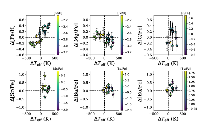
Figure 7: Offsets between the abundances in this paper and those from the literature, as a function of offsets in the adopted effective temperature. Note that the literature atmospheric parameters are all derived in slightly different ways. With the exception of some [Fe/H] ratios, all literature abundances were determined under assumptions of LTE. References for literature abundances are given in the text.

4.2 Abundances of Target Stars

4.2.1 $r$-Process Enhancement

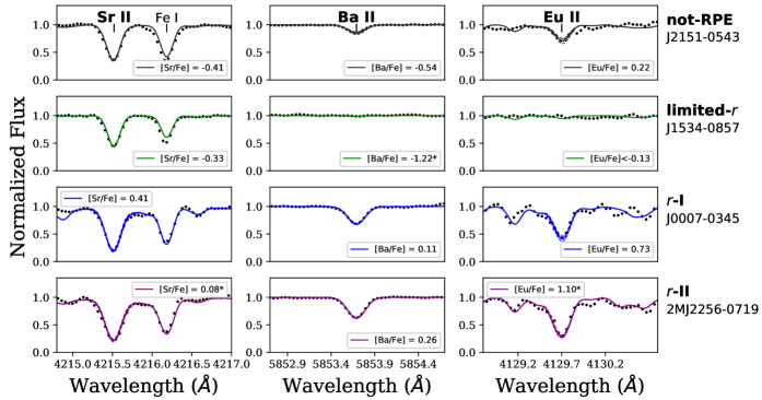
Figure 8: Syntheses of Sr, Ba, and Eu lines in four different stars, one not-RPE, one limited-$r$, one $r$-I, and one $r$-II star. The dashed lines show the $\pm 1\sigma$ errors for a single line. The lines marked with asterisks were not used to determine the abundances, either because they were too strong or too weak in that star; in this case, they are merely shown for illustrative purposes.

The ultimate goal of this paper is to identify $r$-process-enhanced metal-poor stars; particular emphasis is therefore placed on the elements used for this classification, Sr, Ba, and Eu, which are all determined via spectrum syntheses (see Figure 8). The Sr II line at 4077 Å  is frequently too strong for a reliable abundance; conversely, the line at 4161 Å  is frequently too weak. The line at 4215 Å  is generally the best of the three lines, though it is occasionally slightly stronger than the $\rm{REW}=-4.7$ limit. In this case, the Y abundances provide additional constraints on the lighter neutron-capture elements. Ba abundances are determined for all of the stars in the sample, from the Ba II 4554, 5853, 6141, and 6496 Å  lines. The 4554 Å  line is really only sufficiently weak in the hottest ($T\gtrsim 6000$ K) or most barium-poor ($[\rm{Ba/H}]\lesssim-3$) stars. Note that the strong 4554 Å  Ba II and 4077 and 4215 Å  Sr II lines may be affected by NLTE effects; however, Short & Hauschildt (2006) quote an offset in Ba of only $+0.14$ dex in red giant stars, with smaller effects on Sr.

Eu abundances or upper limits are also provided for all stars, from the Eu II 4129, 4205, 4435, and (only in certain cases) 6645 Å  lines. In some cases, the Eu upper limits may not be sufficient to determine if the star is $r$-process-enhanced, particularly if the star is hotter than $\sim 5500$ K. Occasionally, the lower limits in [Ba/Eu] lie below the lower limit for the Solar $r$-process residual; in this case, a second set of limits is also provided in parentheses in Table 5, assuming that $[\rm{Ba/Eu}]~{}>~{}-~{}0.89$ (Burris et al., 2000). Table 5 shows the classifications for the 20 standards and the 126 new targets.

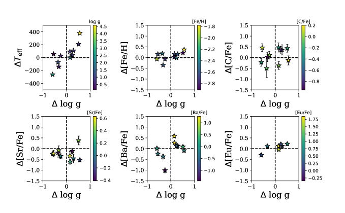
Figure 9: Offsets (this paper $-$ Hansen et al.) between the abundances in this paper and those from Hansen et al. (2018), as a function of the surface gravity (the parameter which varies most between the studies).

Seven of the target stars and three of the standards overlap with the Southern Hemisphere sample from Hansen et al. (2018)—Figure 9 shows the parameter and abundance comparison. The temperatures, [Fe/H], and [Eu/Fe] ratios are generally in good agreement; though Hansen et al. did not employ NLTE corrections, they did use the Frebel et al. (2013) correction to their spectroscopic temperatures. The Sr abundances in this paper are slightly lower, on average, than Hansen et al., and there are occasional disagreements in [Ba/Fe]. Still, the $r$-I and $r$-II classifications match, with one exception: Hansen et al. classify CS 22169-035 as an $r$-I star while here it is classified as limited-$r$.

Table 5: $r$-Process-Enhancement Classifications and Sr, Ba, and Eu Abundance Ratios

Star	Class	[Sr/Fe]		[Ba/Fe]		[Eu/Fe]		[Ba/Eu]		[Sr/Ba]
Standards
CS 31082-001	$r$-II	0.27±0	1.22±0.05  (3)	1.72±0	-0.50±0.07	-0.95±0
TYC 5861-1732-1	not-RPE	-0.48±0	-0.45±0.05  (3)	$<0.29$		$>-0.16$		-0.03±0
CS 22169-035	limited-$r$	-0.07±0	-1.44±0.10  (2)	$<0.01\;\;(<-0.55\tablenotemark{a})$		$>-1.45\;\;(>-0.89)$		1.51±0
TYC 75-1185-1	$r$-I	-0.28±0	0.0±0.05  (3)	0.78±0	-0.78±0.07	-0.28±0
TYC 5911-452-1	not-RPE	-0.23±0	-0.68±0.10  (1)	$<0.72\;\;(<-0.21\tablenotemark{a})$		$>-1.40\;\;(>-0.89)$		0.45±0
TYC 5329-1927-1	$r$-I	-0.07±0	0.13±0.10  (1)	0.89±0	-0.76±0.11	-0.20±0
TYC 6535-3183-1	$r$-I	-0.19±0	-0.19±0.05  (1)	0.31±0	-0.50±0.06	0.00±0
TYC 4924-33-1	not-RPE	-0.21±0	-0.44±0.05  (3)	0.20±0	-0.64±0.15	0.23±0
HE 1116$-$0634	not-RPE	-2.06±0	-2.03±0.20  (1)	$<0.67\;\;(<-1.14\tablenotemark{a})$		$>-2.70\;\;(>-0.89)$		-0.03±0
TYC 6088-1943-1	not-RPE	-0.20±0	-0.48±0.06  (3)	$<0.06$		$>-0.54$		0.28±0
BD$-$13 3442	limited-$r$?	0.15±0	-0.60±0.20  (1)	$<1.70\;\;(<0.29\tablenotemark{a})$		$>-2.30\;\;(>-0.89)$		0.75±0
BD$-$01 2582	CEMP-$s$	0.48±0	1.28±0.05  (3)	0.74±0	0.54±0.06	-0.80±0
HE1317$-$0407	not-RPE	-0.02±0	-0.33±0.03  (3)	0.18±0	-0.51±0.10	0.31±0
HE1320$-$1339	limited-$r$	0.50±0	-0.51±0.04  (2)	-0.08±0	-0.43±0.11	1.01±0
HD 122563	limited-$r$	-0.13±0	-0.92±0.03  (3)	-0.32±0	-0.60±0.06	0.79±0
TYC 4995-333-1	not-RPE	-0.24±0	-0.19±0.05  (3)	0.18±0	-0.37±0.07	-0.05±0
HE 1523$-$0901	$r$-II	0.57±0	1.27±0.05  (1)	1.82±0	-0.55±0.07	-0.70±0
TYC 6900-414-1	$r$-I	-0.68±0	0.08±0.07  (2)	0.49±0	-0.41±0.10	-0.76±0
J2038$-$0023	$r$-II	0.82±0	0.69±0.05  (1)	1.42±0	-0.73±0.11	0.13±0
BD$-$02 5957	$r$-I	0.45±0	0.40±0.04  (3)	0.91±0	-0.51±0.07	0.05±0
Targets
J0007$-$0345	$r$-I	0.41±0	0.11±0.07  (2)	0.73±0	-0.62±0.08	0.41±0
J0012$-$1816	not-RPE	-0.51±0	-0.63±0.05  (3)	$<-0.12$		$>-0.51$		0.12±0
J0022$-$1724	CEMP-no	-0.83±0	-0.73±0.10  (2)	$<2.12\;\;(<0.16\tablenotemark{a})$		$>-2.85\;\;(>-0.89)$		-0.10±0
J0030$-$1007	limited-$r$	0.50±0	-0.71±0.03  (2)	0.0±0	-0.71±0.10	1.21±0
J0053$-$0253	$r$-I	-0.05±0	-0.24±0.03  (2)	0.39±0	-0.63±0.04	0.19±0
J0054$-$0611	$r$-I	0.26±0	-0.21±0.05  (3)	0.59±0	-0.80±0.12	0.47±0
J0107$-$0524	limited-$r$	0.14±0	-0.61±0.06  (3)	$<0.16$		$>-0.77$		0.75±0
J0145$-$2800	limited-$r$	-0.02±0	-1.05±0.06  (2)	$<0.10\;\;(<-0.16\tablenotemark{a})$		$>-1.15\;\;(>-0.89)$		1.03±0
J0156$-$1402	$r$-I	0.10±0	-0.11±0.10  (1)	0.76±0	-0.87±0.12	0.21±0
J0213$-$0005	not-RPE	-0.54±0	0.05±0.07  (2)	$<0.16$		$>-0.11$		-0.59±0
J0227$-$0519	$r$-I	0.72±0	-0.18±0.10  (1)	0.42±0	-0.60±0.12	0.90±0
J0229$-$1307	?	-0.37±0	-0.32±0.07  (2)	$<0.95\;\;(<0.57\tablenotemark{a})$		$>-1.27\;\;(>-0.89)$		-0.05±0
J0236$-$1202	not-RPE	-0.41±0	-0.29±0.08  (3)	¡0.30	¿-0.59	-0.12±0
J0241$-$0427	$r$-I	0.24±0	-0.26±0.06  (3)	0.48±0	-0.74±0.09	0.50±0
J0242$-$0707	?	0.37±0	-0.08±0.10  (1)	$<1.04$ ($<0.82$)		$>-1.12$ ($>-0.89$)		0.45±0
J0243$-$3249	not-RPE?	$<-0.59$		-0.95±0	$<0.93$ ($<0.05$)		$>-1.88$ ($>-0.89$)		$<0.36$
J0246$-$1518	$r$-II	0.33±0	0.65±0.06  (3)	1.29±0	-0.64±0.09	-0.42±0
J0307$-$0534	$r$-I	0.38±0	0.17±0.06  (3)	0.50±0	-0.33±0.09	0.21±0
J0313$-$1020	$r$-I	-0.17±0	-0.12±0.06  (3)	0.42±0	-0.54±0.09	-0.05±0
J0343$-$0924	$r$-I	-0.02±0	-0.07±0.10  (1)	0.38±0	-0.45±0.12	0.05±0
J0346$-$0730	not-RPE	0.11±0	-0.19±0.06  (3)	0.16±0	-0.35±0.08	0.30±0
J0355$-$0637	limited-$r$	0.50±0	-0.28±0.07  (2)	0.25±0	-0.53±0.10	0.78±0
J0419$-$0517	$r$-I	0.23±0	0.0±0.10  (1)	0.40±0	-0.40±0.12	0.23±0
J0423$-$1315	not-RPE	-0.24±0	-0.29±0.10  (1)	0.08±0	-0.37±0.18	0.05±0
J0434$-$2325	limited-$r$?	-0.42±0	-2.27±0.11  (2)	$<-0.53$ ($<-1.38$)		$>-1.74$ ($>-0.89$)		1.85±0
J0441$-$2303	?	-0.22±0	-0.41±0.13  (2)	$<0.55$ ($<0.48$)		$>-0.96$ ($>-0.89$)		0.19±0
J0453$-$2437	$r$-I	-0.21±0	-0.04±0.07  (3)	0.59±0	-0.63±0.09	-0.17±0
J0456$-$3115	$r$-I	0.02±0	-0.33±0.10  (1)	0.34±0	-0.67±0.14	0.35±0
J0505$-$2145	not-RPE	-0.22±0	-0.32±0.07  (2)	0.15±0	-0.47±0.11	0.10±0
J0517$-$1342	not-RPE	-0.43±0	-0.43±0.06  (3)	0.21±0	-0.64±0.09	0.0±0
J0525$-$3049	not-RPE	0.40±0	0.02±0.07  (2)	0.12±0	-0.10±0.21	0.38±0
J0610$-$3141	limited-$r$?	-0.37±0	-1.57±0.10  (1)	$<1.30$ ($<-0.68$)		$>-2.87$ ($>-0.89$)		1.20±0
J0705$-$3343	$r$-I	0.03±0	-0.17±0.06  (3)	0.62±0	-0.79±0.09	0.20±0
J0711$-$3432	$r$-II	$<0.24$	0.50±0.06  (3)	1.30±0	-0.80±0.12	$<-0.26$
J0910$-$1444	limited-$r$	-0.20±0	-1.64±0.09  (2)	$<0.03$ ($<-0.78$)		$>-1.67$ ($>-0.89$)		1.44±0
J0918$-$2311	$r$-I	-0.51±0	-0.06±0.10  (1)	0.71±0	-0.77±0.13	-0.45±0
J0929$-$2905	not-RPE	-0.36±0	-0.37±0.06  (3)	0.14±0	-0.51±0.10	0.01±0
J0946$-$0626	$r$-I	0.03±0	-0.07±0.07  (2)	0.35±0	-0.42±0.11	0.10±0
J0949$-$1617	CEMP-$r$/$s$	0.16±0	0.61±0.10  (1)	0.36±0	0.25±0.12	-0.45±0
J0950$-$2506	not-RPE	-0.42±0	-0.57±0.07  (2)	¡0.10	¿-0.67	0.15±0
J0952$-$0855	limited-$r$	0.00±0	-1.05±0.05  (3)	$<0.24$ ($<-0.16$)		$>-1.29$ ($>-0.89$)		1.05±0
J0958$-$1446	$r$-I	0.59±0	0.20±0.15  (2)	0.59±0	-0.39±0.16	0.39±0
J1004$-$2706	$r$-I	0.0±0	-0.38±0.06  (3)	0.41±0	-0.79±0.09	0.38±0
J1022$-$3400	$r$-I	0.35±0	-0.29±0.06  (3)	0.37±0	-0.66±0.08	0.64±0
J1031$-$0827	not-RPE	0.24±0	-0.23±0.06  (3)	0.26±0	-0.49±0.23	0.47±0
J1036$-$1934	limited-$r$	0.22±0	-0.38±0.06  (3)	0.26±0	-0.64±0.08	0.60±0
J1049$-$1154	$r$-I	-0.06±0	-0.16±0.06  (3)	0.33±0	-0.49±0.09	0.10±0
J1051$-$2115	$r$-I	0.03±0	-0.27±0.07  (2)	0.32±0	-0.59±0.10	0.30±0
J1059$-$2052	$r$-I	0.26±0	-0.07±0.06  (3)	0.35±0	-0.42±0.08	0.33±0
J1120$-$2406	not-RPE	-0.16±0	-0.17±0.06  (3)	$<0.16$		$>-0.33$		0.01±0
J1124$-$2155	not-RPE	0.20±0	-0.17±0.06  (3)	0.22±0	-0.39±0.09	0.37±0
J1130$-$1449	$r$-I	0.08±0	-0.12±0.06  (3)	0.50±0	-0.62±0.09	0.20±0
J1139$-$0558	not-RPE	-0.10±0	-0.30±0.06  (3)	0.29±0	-0.59±0.09	0.20±0
J1144$-$0409	$r$-I	-0.01±0	-0.26±0.07  (2)	0.58±0	-0.84±0.09	0.25±0
2MJ1144$-$1128	$r$-I	0.03±0	-0.29±0.06  (3)	0.35±0	-0.64±0.09	0.32±0
J1146$-$0422	CEMP-$r$	-0.28±0	0.32±0.10  (1)	0.62±0	-0.30±0.12	-0.60±0
J1147$-$0521	$r$-I	0.0±0	-0.22±0.06  (3)	0.31±0	-0.53±0.08	0.22±0
J1158$-$1522	limited-$r$	-0.37±0	-1.07±0.14  (2)	$<0.15$ ($<-0.18$)		$>-1.22$ ($>-0.89$)		0.70±0
J1204$-$0759	$r$-I	-0.29±0	-0.11±0.06  (3)	0.33±0	-0.44±0.21	-0.18±0
2MJ1209$-$1415	$r$-I	-0.01±0	0.11±0.13  (2)	0.81±0	-0.70±0.14	-0.12±0
J1218$-$1610	limited-$r$	-0.20±0	-1.50±0.20  (1)	$<0.17$ ($<-0.61$)		$>-1.67$ ($>-0.89$)		1.30±0
J1229$-$0442	$r$-I	0.0±0	-0.22±0.06  (3)	0.46±0	-0.68±0.07	0.22±0
J1237$-$0949	not-RPE	0.22±0	-0.27±0.07  (2)	0.19±0	-0.46±0.09	0.49±0
J1250$-$0307	$r$-I	-0.57±0	0.10±0.06  (3)	0.45±0	-0.35±0.13	-0.67±0
J1256$-$0834	$r$-I	0.32±0	-0.28±0.07  (2)	0.45±0	-0.73±0.09	0.60±0
J1302$-$0843	$r$/$s$	$<0.73$	0.55±0.07  (1)	0.41±0	0.14±0.09	¡0.18
J1306$-$0947	not-RPE	-0.21±0	-0.12±0.04  (3)	0.12±0	-0.24±0.08	-0.09±0
2MJ1307$-$0931	not-RPE	0.02±0	-0.38±0.05  (3)	0.10±0	-0.48±0.08	0.40±0
J1321$-$1138	not-RPE	-0.03±0	-0.36±0.06  (3)	0.08±0	-0.44±0.09	0.33±0
2MJ1325$-$1747	$r$-I	-0.02±0	-0.44±0.07  (2)	0.40±0	-0.84±0.09	0.42±0
J1326$-$1525	limited-$r$	-0.10±0	-0.67±0.06  (3)	-0.28±0	-0.39±0.12	0.57±0
J1328$-$1731	not-RPE	-0.02±0	-0.08±0.06  (3)	0.20±0	-0.28±0.13	0.06±0
J1333$-$2623	limited-$r$	0.11±0	-0.55±0.06  (3)	0.20±0	-0.75±0.10	0.66±0
J1335$-$0110	$r$-I	-0.39±0	-0.22±0.05  (3)	0.53±0	-0.75±0.09	-0.17±0
J1337$-$0826	$r$-I	0.17±0	0.02±0.02  (3)	0.93±0	-0.91±0.11	0.15±0
J1339$-$1257	not-RPE	0.08±0	-0.42±0.06  (3)	0.10±0	-0.52±0.21	0.27±0
2MJ1340$-$0016	not-RPE	0.05±0	-0.30±0.06  (3)	0.29±0	-0.59±0.13	0.35±0
J1342$-$0717	$r$-I	0.04±0	-0.26±0.06  (3)	0.44±0	-0.70±0.08	0.30±0
2MJ1343$-$2358	CEMP-no	-0.37±0	-0.77±0.07  (2)	$<0.15$ ($<0.12$)		$>-0.92$ ($>-0.89$)		0.40±0
J1403$-$3214	not-RPE	-0.60±0	-0.08±0.06  (2)	0.12±0	-0.20±0.12	-0.52±0
2MJ1404$+$0011	CEMP-$r$	0.43±0	0.38±0.07  (2)	0.58±0	-0.28±0.09	0.05±0
J1410$-$0343	$r$-I	-0.15±0	-0.12±0.06  (3)	0.67±0	-0.79±0.09	-0.03±0
J1416$-$2422	not-RPE	0.02±0	-0.31±0.06  (3)	0.14±0	-0.45±0.12	0.33±0
J1418$-$2842	$r$-I	-0.41±0	-0.11±0.06  (3)	0.43±0	-0.54±0.13	-0.30±0
J1419$-$0844	$r$-I	0.34±0	-0.15±0.06  (3)	0.34±0	-0.49±0.08	0.49±0
J1500$-$0613	$r$-I	0.12±0	-0.10±0.06  (3)	0.39±0	-0.49±0.08	0.32±0
J1502$-$0528	not-RPE	0.02±0	0.00±0.06  (3)	0.24±0	-0.24±0.08	0.02±0
J1507$-$0659	$r$-I	0.12±0	-0.10±0.06  (3)	0.36±0	-0.46±0.08	0.22±0
J1508$-$1459	$r$-I	0.0±0	-0.10±0.06  (3)	0.49±0	-0.59±0.09	0.10±0
J1511$+$0025	$r$-I	0.02±0	-0.18±0.06  (3)	0.41±0	-0.59±0.08	0.20±0
J1516$-$2122	CEMP-no	-0.03±0	-0.48±0.06  (3)	0.09±0	-0.59±0.09	0.45±0
2MJ1521$-$0607	$r$-I	-0.18±0	0.10±0.07  (2)	0.93±0	-0.83±0.10	-0.28±0
J1527$-$2336	?	-0.18±0	-0.11±0.07  (2)	¡0.74	¿-0.85	-0.07±0
J1534$-$0857	limited-$r$	-0.33±0	-1.22±0.05  (3)	$<-0.13$ ($<-0.33$)		$>-1.09$ ($>-0.89$)		0.89±0
J1538$-$1804	$r$-II	0.44±0	0.62±0.07  (2)	1.27±0	-0.65±0.09	-0.18±0
J1542$-$0131	not-RPE	0.02±0	-0.35±0.06  (3)	0.26±0	-0.61±0.09	0.37±0
J1547$-$0837	limited-$r$	0.78±0	-0.50±0.06  (3)	-0.10±0	-0.40±0.15	1.28±0
J1554$+$0021	not-RPE	0.19±0	-0.26±0.06  (3)	-0.09±0	-0.17±0.09	0.45±0
J1602$-$1521	not-RPE	0.10±0	0.09±0.06  (3)	0.25±0	-0.16±0.08	0.01±0
J1606$-$0400	not-RPE	-0.02±0	-0.17±0.07  (2)	0.23±0	-0.40±0.11	0.15±0
J1606$-$1632	limited-$r$	0.01±0	-0.57±0.07  (2)	-0.27±0	-0.30±0.12	0.58±0
J1609$-$0941	$r$-I	-0.06±0	-0.30±0.05  (3)	0.41±0	-0.71±0.08	0.24±0
J1612$-$0541	not-RPE	0.07±0	0.03±0.06  (3)	0.20±0	-0.17±0.09	0.00±0
J1612$-$0848	$r$-I	0.29±0	0.04±0.06  (3)	0.58±0	-0.54±0.08	0.25±0
J1616$-$0401	$r$-I	0.08±0	-0.19±0.07  (3)	0.52±0	-0.71±0.09	0.27±0
J1618$-$0630	not-RPE?	0.01±0	-0.59±0.10  (1)	¡-0.27	¿-0.32	0.58±0
J1627$-$0848	not-RPE	0.00±0	0.10±0.06  (3)	0.12±0	-0.02±0.21	-0.10±0
J1628$-$1014	$r$-I	-0.26±0	-0.02±0.06  (3)	0.36±0	-0.38±0.08	-0.24±0
J1639$-$0522	limited-$r$	0.36±0	-0.26±0.06  (3)	-0.07±0	-0.19±0.21	0.62±0
J1645$-$0429	limited-$r$	0.38±0	-0.37±0.06  (3)	-0.15±0	-0.22±0.12	0.75±0
J1811$-$2126	not-RPE	-0.09±0	0.18±0.10  (1)	0.28±0	-0.10±0.14	-0.27±0
J1905$-$1949	$r$-I	-0.01±0	-0.08±0.03  (3)	0.36±0	-0.44±0.05	0.07±0
J2005$-$3057	$r$-I	-0.16±0	0.36±0.07  (2)	0.86±0	-0.50±0.10	-0.52±0
J2010$-$0826	$r$-I	0.04±0	-0.39±0.04  (3)	0.42±0	-0.81±0.08	0.43±0
J2032$+$0000	not-RPE	0.16±0	-0.29±0.07  (2)	0.26±0	-0.55±0.10	0.45±0
J2036$-$0714	CEMP-$r$	0.02±0	-0.57±0.10  (1)	0.48±0	-0.87±0.12	0.59±0
J2038$-$0252	$r$-I	0.39±0	-0.26±0.10  (1)	0.59±0	-0.85±0.12	0.65±0
J2054$-$0033	CEMP-no/lim-$r$	0.63±0	-0.27±0.06  (3)	¡-0.18	¿-0.14	0.90±0
J2058$-$0354	$r$-I	-0.24±0	-0.09±0.06  (3)	0.36±0	-0.45±0.08	-0.15±0
J2116$-$0213	$r$-I	-0.41±0	-0.31±0.10  (1)	0.60±0	-0.91±0.12	-0.10±0
J2151$-$0543	not-RPE	-0.41±0	-0.54±0.06  (3)	0.22±0	-0.76±0.09	0.13±0
2MJ2256$-$0719	$r$-II	0.08±0	0.26±0.04  (3)	1.10±0	-0.84±0.08	-0.18±0
J2256$-$0500	not-RPE	-0.10±0	-0.46±0.06  (3)	-0.06±0	-0.40±0.09	0.36±0
J2304$+$0155	not-RPE	0.01±0	-0.20±0.07  (2)	0.26±0	-0.45±0.10	0.21±0
J2325$-$0815	$r$-I	-0.42±0	-0.33±0.07  (2)	0.55±0	-0.88±0.10	-0.09±0

4.2.2 Other Neutron-Capture Abundances

Abundances of other neutron-capture elements are given in Table 6. Abundances of Y, La, Ce, and Nd are available for most of the stars, while Zr, Pr, Sm, Dy, and Os are only available in the stars with high S/N, higher [Fe/H], and/or high $r$-process enhancement. Th is heavily blended, and was only detectable in a handful of stars. Abundances of all these elements were determined with spectrum syntheses.

Table 6: Elemental Abundances

Star	[O/Fe]	[Na/Fe]	[Mg/Fe]	[Si/Fe]	[K/Fe]	[Ca/Fe]	[Sc/Fe]	[Ti I/Fe]		[V/Fe]	[Cr II/Fe]	[Mn/Fe]	[Co/Fe]	[Ni/Fe]	[Cu/Fe]	[Zn/Fe]	[Y/Fe]	[Zr/Fe]		[Ce/Fe]	[Pr/Fe]	[Nd/Fe]	[Sm/Fe]	[Dy/Fe]	[Os/Fe]	[Th/Fe]
CS 31082-001	—	—	$0.46\pm 0.04$ (4)	—	$0.17\pm 0.10$ (1)	$0.44\pm 0.01$ (23)	$-0.03\pm 0.04$ (5)	$0.20\pm 0.01$ (14)		—	$0.37\pm 0.10$ (1)	—	$0.03\pm 0.10$ (1)	$0.03\pm 0.05$ (5)	—	$0.15\pm 0.10$ (1)	$0.45\pm 0.05$ (6)	$0.62\pm 0.10$ (1)		$1.04\pm 0.05$ (6)	$1.24\pm 0.06$ (4)	$1.29\pm 0.05$ (8)	$1.42\pm 0.05$ (1)	$1.22\pm 0.10$ (1)	$1.65\pm 0.07$ (2)	—
T5861-1732-1	—	$0.50\pm 0.05$ (2)	$0.42\pm 0.04$ (3)	$0.52\pm 0.10$ (1)	$0.34\pm 0.10$ (1)	$0.31\pm 0.01$ (24)	$-0.15\pm 0.02$ (10)	$0.07\pm 0.01$ (17)		—	$-0.01\pm 0.05$ (4)	—	$-0.20\pm 0.11$ (2)	$-0.11\pm 0.01$ (12)	—	$0.03\pm 0.13$ (2)	$-0.41\pm 0.08$ (2)	—		—	—	—	—	—	—	—
CS 22169-035	—	—	$0.32\pm 0.03$ (2)	—	$0.31\pm 0.10$ (1)	$0.18\pm 0.01$ (12)	$-0.25\pm 0.03$ (5)	$-0.12\pm 0.01$ (6)		—	—	$-0.27\pm 0.10$ (1)	$0.22\pm 0.06$ (2)	$0.10\pm 0.03$ (5)	—	—	$-0.39\pm 0.05$ (2)	—		—	—	—	—	—	—	—
T75-1185-1	—	—	$0.30\pm 0.09$ (2)	—	$0.30\pm 0.10$ (1)	$0.35\pm 0.01$ (16)	$-0.10\pm 0.04$ (5)	$0.27\pm 0.02$ (15)		—	$0.22\pm 0.10$ (1)	$-0.29\pm 0.02$ (2)	$-0.04\pm 0.02$ (3)	$0.17\pm 0.02$ (5)	—	$0.10\pm 0.10$ (1)	$-0.20\pm 0.07$ (3)	—		—	—	—	—	—	—	—
T5911-452-1	—	—	$0.32\pm 0.03$ (2)	—	$0.45\pm 0.10$ (1)	$0.26\pm 0.02$ (14)	$0.04\pm 0.02$ (3)	$0.39\pm 0.04$ (5)		—	—	—	—	$0.09\pm 0.10$ (1)	—	—	—	—		—	—	—	—	—	—	—

4.2.3 The $\alpha$-Elements and K

In most of the stars there are many clear Ca I, Ti I, and Ti II lines; the Ca and Ti abundances were therefore determined differentially with respect to a standard, similar to Fe I and Fe II. Note that the Ti lines follow similar trends as the Fe lines when NLTE corrections are not applied, i.e., the Ti I lines yield lower Ti abundances than the Ti II abundances. Because the [Ti I/H] ratios are likely to be too low, the average differential offsets in [Ti I/H] and [Ti II/H] are both applied relative to the [Ti II/H] ratios in the standard stars.

The other elements were not determined differentially. The Mg I lines at 4057, 4167, 4703, 5528, and 5711 Å  are generally detectable, though at the metal-rich end some become prohibitively strong. The Si I lines are generally very weak in metal-poor stars, and are occasionally difficult to detect even in high S/N spectra. The K I line at 7699 Å  lies at the edge of a series of telluric absorption lines; when the K line is distinct from the telluric features a measurement is provided. In a handful of stars, the O abundance can be determined from the 6300 and 6363 Å  forbidden lines.

4.2.4 Iron-peak Elements, Cu, and Zn

Abundances of Sc II, V I, Cr II, Mn I, Co I, and Ni I were all determined from EWs, considering HFS when necessary. Each species has a multitude of available lines. Note that Cr I lines are not included, as they are expected to suffer from NLTE effects (Bergemann & Cescutti, 2010). The Mn lines in these metal-poor stars may require NLTE corrections $\sim 0.5-0.7$ dex (Bergemann & Gehren, 2008), but they have not been applied here.

Cu and Zn were determined via spectrum syntheses, using the 5105 and 5782 Å  Cu I lines and the 4722 and 4810 Å  Zn I lines. Note that the Cu I lines are likely to suffer from NLTE issues (e.g., Shi et al. 2018); these corrections are also not applied here.

4.2.5 Light Elements: Li and Na

In some stars, Na abundances can be determined from the Na I doublet at 5682/5688 Å. In the most metal-poor stars, the Na I doublet at 5889 and 5895 Å  is weak enough for an abundance determination, but is only used if the interstellar contamination is either insignificant or is sufficiently offset from the stellar lines. Note that the NaD lines may suffer from NLTE effects (e.g., Andrievsky et al. 2007), but the 5682/5688 Å  lines are not likely to have significant NLTE corrections in this metallicity range (Lind et al., 2011).

The Li I line at 6707 Å  is detectable in nine stars, as listed in Table 7. These Li abundances are typical for the evolutionary state of the stars; the main sequence stars have values that are consistent with the Spite plateau, while the giants show signs of Li depletion. Two $r$-II, three $r$-I, and one limited-$r$ stars have Li detections.

Table 7: Stars with Li Measurements

Star	$\log\epsilon$ (Li)	$T_{\rm{eff}}$ (K)
J0107$-$0524	$1.20\pm 0.05$	5225
2MJ0213$-$0005	$2.42\pm 0.05$	6225
J0517$-$1342	$0.91\pm 0.10$	4961
J0705$-$3343	$0.81\pm 0.10$	4757
J0711$-$3432	$0.94\pm 0.10$	4767
J1022$-$3400	$0.79\pm 0.05$	4831
J1333$-$2623	$0.94\pm 0.05$	4821
J1527$-$2336	$2.46\pm 0.10$	6260
J1538$-$1804	$0.81\pm 0.05$	4752
J2058$-$0354	$0.89\pm 0.05$	4831

5 Discussion

5.1 The $r$-process-Enhanced Stars

Figure 10 shows [Eu/Fe], [Mg/Fe], [Ba/Eu], and [Sr/Ba] as a function of [Fe/H], grouped by their $r$-process enhancement. This northern survey has discovered 4 new $r$-II stars, including J1538$-$1804 (published by Sakari et al. 2018), 60 new $r$-I stars (three of them CEMP-$r$), and 19 new limited-$r$ stars. Combined with the results from Hansen et al. (2018), Placco et al. (2017), Gull et al. (2018), Holmbeck et al. (2018a), Cain et al. (2018), and Roederer et al. (2018b), the RPA has so far identified, in total, 18 new $r$-II, 101 new $r$-I (including 6 CEMP-$r$), 39 limited-$r$, and 1 $r+s$ star. The properties of the stars from this paper are discussed below.

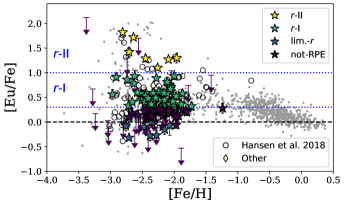
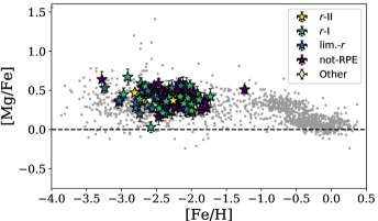
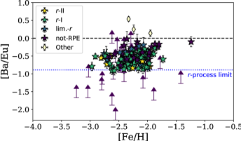
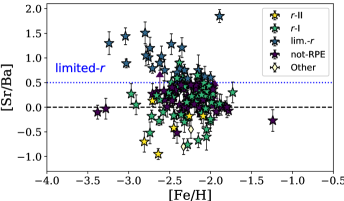
Figure 10: Ratios of [Eu/Fe], [Mg/Fe], [Ba/Eu], and [Sr/Ba] as a function of [Fe/H]. The standard and target stars are grouped by $r$-process enhancement. “Other” includes stars with $s$ and $r/s$ classifications. For reference, the Hansen et al. (2018) stars are shown as open circles, while MW field stars from Venn et al. (2004) and Reddy et al. (2006) are shown as gray dots. In the top left plot, the $r$-I and $r$-II limits in [Eu/Fe] are shown with a dotted line. The Solar $r$-process [Ba/Eu] ratio from Burris et al. (2000) is indicated in the bottom left plot. Finally, in the bottom right panel, the limit for the limited-$r$ stars, [Sr/Ba]$>+0.5$, is shown.

5.1.1 The Sub-populations of $r$-process-Enhanced Stars

The metallicity distribution of the different $r$-process sub-populations is very similar to that found in Hansen et al. (2018), as shown in Figure 11. The $r$-I and $r$-II stars are found across the full [Fe/H] range; there is a hint that the limited-$r$ stars are only found at lower metallicities, but more stars are necessary to validate this.

Figure 11 shows the distribution of [Ba/Eu] values. The $r$-II stars and many of the $r$-I stars have low [Ba/Eu], consistent with little enrichment from the main $s$-process. The not-RPE and limited-$r$ stars seem to extend to higher [Ba/Eu], indicating some amount of $s$-process contamination. Figure 10 also demonstrates that the $r$-II stars have low [Sr/Ba]. As in the Hansen et al. sample, some $r$-I stars are found to have enhanced [Sr/Ba] and [Sr/Eu] ratios, similar to the stars in the limited-$r$ class.

Note that the large spread in [Eu/Fe] at a given metallicity is not accompanied by a similar spread in [Mg/Fe] (see Figure 10), which has been noted by many other authors. With one exception, all the target stars have light, $\alpha$, and Fe-peak abundances that are consistent with normal MW halo stars, regardless of $r$-process enhancement. This places important constraints on the nucleosynthetic signature and site of the $r$-process. For instance, the robust Mg abundances rule out traditional core-collapse supernovae as the only source of the heavy $r$-process elements (also see Macias & Ramirez-Ruiz 2016).

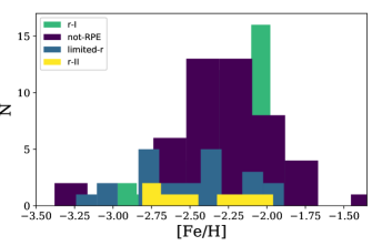
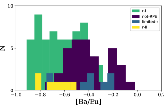
Figure 11: Histograms showing the [Fe/H] (left) and [Ba/Eu] (right) distributions for the different groups of stars. The stars with $s$- or $r$/$s$-process signatures have been removed.

5.1.2 Kinematics

All of these stars are Gaia DR2 targets; all but one have proper motions and parallaxes, though the parallax errors are occasionally too large to provide reliable distances (Bailer-Jones et al., 2018). Figure 12 shows a Toomre diagram for stars with parallax errors $<20$%, generated with the gal_uvw code. This diagram distinguishes between disk and halo stars, and between retrograde and prograde halo stars. The errors in Figure 12 reflect the uncertainties in the parallax and proper motion. The velocities have been corrected for the solar motion, according to the values from Coşkunoǧlu et al. (2011).

In Figure 12 the stars are grouped by their $r$-process-enhancement classification, and are compared with kinematically-selected MW halo stars from Koppelman et al. (2018). Several of the non-RPE stars are consistent with membership in the metal-weak thick disk (Kordopatis et al., 2013b). The majority of the $r$-process-enhanced stars are consistent with membership in the halo, and a large number are retrograde halo stars. All of the $r$-II stars and more than half of the $r$-I stars in this paper are retrograde, possibly indicating they originated in a satellite. The kinematics of three of the $r$-II stars from Hansen et al. (2018) are presented in Roederer et al. (2018a); only those three pass the stringent cut in parallax error, but note that two of these stars are prograde halo stars. The kinematics of $r$-process-enhanced stars will have important consequences for the birth sites of these stars. Full orbital calculations will be even more useful (Roederer et al., 2018a).

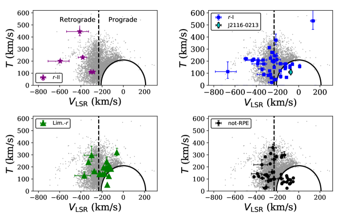
Figure 12: Toomre diagrams for the four main sub-populations in this paper, where $T=\sqrt{U^{2}+W^{2}}$. This plot helps distinguish halo stars from disk stars and retrograde halo stars from prograde halo stars. The gray points show MW disk and halo stars within 1 kpc from Koppelman et al. (2018)—the large circle shows their criterion for halo membership; disk stars lie within the circle. The colored points use Gaia DR2 data; when radial velocities were not available, the values from this paper were used. Only stars with parallax uncertainties $<20$% are shown (see Bailer-Jones et al. 2018). The upper left panel shows the $r$-II stars, the upper right panel the $r$-I stars, the lower left panel the limited-$r$ stars, and the lower right panel the “not-RPE” stars.

5.1.3 Detailed $r$-process Patterns

Figure 13(a) shows the detailed $r$-process patterns and residuals with respect to the scaled-Solar $r$-process pattern in three $r$-II stars (the pattern for J1538$-$1804 was presented in Sakari et al. 2018). As has been found in numerous other studies, the abundance patterns are consistent with the scaled-Solar $r$-process pattern (but see below for Th). Figure 13(b) shows patterns for six of the $r$-I stars. The top two panels show $r$-I stars with low [Ba/Eu] and [Sr/Ba]; as expected, their abundances are consistent with a pure $r$-process pattern. The next two panels show $r$-I stars with low [Ba/Eu], but elevated [Sr/Ba]. These stars have elevated Sr, Y, and Zr compared to the scaled-Solar pattern, but the pattern of the lanthanides is consistent. Finally, the last two panels show $r$-I stars with slightly sub-Solar [Ba/Eu], indicating some $s$-process contamination. These stars have high Sr, Y, Zr, Ba, La, and Ce, relative to the Solar pattern.

These detailed patterns support the classifications from the more general [Ba/Eu] and [Sr/Ba] ratios (e.g., Frebel 2018; Spite et al. 2018), and will be useful in identifying the nucleosynthetic signatures of the limited-$r$ and $r$-processes. Follow-up of the limited-$r$ and $r$-I stars with enhanced [Sr/Ba] will enable detailed comparisons between abundance patterns and model predictions, particularly in the 38 $\leq Z\leq$ 47 range, which could distinguish between limited-$r$ and weak $s$-process scenarios (e.g., Chiappini et al. 2011; Frischknecht et al. 2012; Cescutti et al. 2013; Frischknecht et al. 2016).

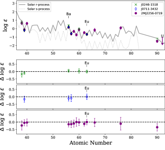
(a) $r$-II stars

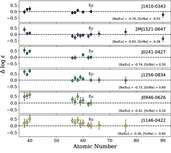
(b) $r$-I stars

Figure 13: Detailed $r$-process patterns for new $r$-II (left) and $r$-I (right) stars compared to the Solar $r$-process residual from Arlandini et al. (1999). The points have been shifted to common Eu abundances. The $r$-I stars are grouped by [Ba/Eu] and [Sr/Ba], demonstrating pure $r$-process enrichment in the top two panels, limited-$r$ enhancement in Sr, Y, and Zr in the middle two panels, and $s$-process enhancement in the bottom two panels.

5.1.4 Cosmochronometric Ages

The few $r$-I and $r$-II stars with Th detections enable determinations of 1) cosmo-chronometric ages and 2) the possible presence of an actinide boost. Table 8 shows the Th abundances relative to Eu and ages derived from Equation 1 in Placco et al. (2017), using two different sets of production ratios: the Schatz et al. (2002) values, from waiting-point calculations, and the Hill et al. (2017) values, from a high-entropy wind. Although the errors in age are quite large (due to high uncertainties in the Th abundance), all of the stars have Th/Eu ratios that are consistent with ancient $r$-process production; none appear to exhibit an actinide boost. Several of the ages are quite old, comparable to the results found for Reticulum II (Ji & Frebel, 2018). These old ages are consistent with recent results from simulations, which suggest that many of the most metal-poor MW halo stars should be ancient (Starkenburg et al., 2017; El-Badry et al., 2018). These ages will be greatly improved through higher precision Th abundances and U detections, which require observations at higher resolution and higher S/N.

Table 8: Th/Eu Abundance Ratios and Ages

					Age (Gyr)
Star	[Fe/H]		$\log\epsilon$ (Th/Eu)		Schatz et al. (2002)	Hill et al. (2017)
J0053$-$0253	-2.16±0	-0.61±0.11	13.1±5	17.3±5.1
J0246$-$1518	-2.45±0	¡-0.70	¿17.3	¿21.5
J0313$-$1020	-2.05±0	-0.58±0.21	11.2±9	15.9±9.8
J0343$-$0924	-1.92±0	-0.58±0.17	11.2±7	15.9±7.9
J1410$-$0343	-2.06±0	-0.65±0.21	14.9±9	19.1±9.8
2MJ1521$-$0607	-2.00±0	-0.75±0.17	19.6±7	23.8±7.9
2MJ2256$-$0719	-2.26±0	-0.76±0.20	20.1±9	24.3±9.3

5.2 J2116$-$0213: A Globular Cluster Star?

One of the $r$-I stars in this sample, J2116$-$0213, has elevated sodium ($[\rm{Na/Fe}]=+0.68\pm 0.07$) and has low magnesium ($[\rm{Mg/Fe}]~{}=~{}+~{}0.03\pm 0.05$; see Figure 14) coupled with normal Si, Ca, and Ti. The Al lines at 6696 and 6698 Å  are too weak for a robust [Al/Fe] measurement. These abundances are not like typical halo stars; instead, this abundance pattern is a signature of multiple populations in globular clusters (GCs; e.g., Carretta et al. 2009). This suggests that J2116$-$0213 may have originated in a GC and was later ejected into the Milky Way halo. Escaped GC stars have been identified from their unique abundance signatures in the MW halo (Martell et al., 2016) and bulge (Schiavon et al., 2017). J2116$-$0213 is an $r$-I star with $[\rm{Eu/Fe}]~{}\sim~{}+~{}0.6$—this is consistent with other metal-poor GCs, which contain large numbers of $r$-I stars (Gratton et al., 2004). However, J2116$-$0213 is more metal-poor ($[\rm{Fe/H}]\sim-2.6$) than the intact MW GCs. Note that this star’s location in the Toomre diagram is right between the thick halo/halo classification; a more detailed orbit for this star could potentially identify its birth environment more clearly.

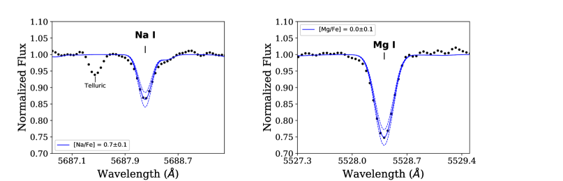
Figure 14: Syntheses to the 5688 Å  Na I and 5528 Å  Mg I lines in J2116$-$0213. Uncertainties of $\pm 0.1$ dex are shown.

6 Conclusions

This paper has presented high-resolution spectroscopic observations of 126 new metal-poor stars and 20 previously observed standards, as part of the $R$-Process Alliance (also see Hansen et al. 2018). Atmospheric parameters and metallicities were derived differentially with respect to a set of standards, applying $<$3D$>$ NLTE corrections. Abundances of a wide variety of elements were then determined. Sr, Ba, and Eu were used to classify the stars according to their $r$-process enhancement, using [Eu/Fe] as the indicator of the main $r$-process, [Ba/Eu] as the indicator for the amount of main $s$-process contamination, and [Sr/Ba] as the indicator for the amount of limited-$r$ (or weak-$s$) contamination. Proper motions and parallaxes from Gaia DR2 enabled the 3D kinematics of these stars to be probed.

Out of the 126 metal-poor targets, four were discovered to be highly Eu-enhanced $r$-II stars. All four are found to have $r$-process patterns that are consistent with the scaled Solar $r$-process residual, and all show no signs of significant contributions from the limited-$r$ or $s$-processes. In other words, the $r$-II stars have retained a pure main $r$-process signature, even though they span a large range in metallicity. All the $r$-II stars in this paper have retrograde halo orbits. The 60 new $r$-I stars show more variation; some exhibit a limited-$r$ signature and some have contributions from the $s$-process, but many have low [Ba/Eu] and [Sr/Ba] ratios consistent with a pure $r$-process signal. As with the $r$-II stars, the $r$-I stars span a wide range in [Fe/H]. The majority of the $r$-I stars are likely halo stars, many of them with retrograde orbits. The smaller number of limited-$r$ stars prohibits making firm conclusions about them as a stellar population, but the 19 in this paper are restricted to lower metallicities.

A number of interesting individual stars were identified in this survey, most of which are being targeted for follow-up observations at higher spectral resolution. Nine CEMP stars were discovered: three are $r$-I stars, four are CEMP-no, and two are CEMP-$r/s$. Another star was found to have an $r/s$ signature, but its corrected C abundance ratio, $[\rm{C/Fe}]~{}=~{}+~{}0.67$, lies slightly below the CEMP threshold. An $r$-I star, J2116$-$0213, is also found to have high [Na/Fe] and low [Mg/Fe], a characteristic sign of the “intermediate” or “extreme” populations in GCs (Carretta et al., 2009). J2116$-$0213 may therefore have been accreted from a very metal-poor globular cluster.

These results are part of an ongoing survey by the RPA to assess the $r$-process-enhancement phenomenon in MW halo stars. The first two releases from the Northern (this paper) and Southern Hemisphere (Hansen et al., 2018) observing campaigns have significantly increased the numbers of known $r$-I, $r$-II, and limited-$r$ stars. By incorporating the kinematic information from Gaia, these stars can start to be investigated as stellar populations rather than interesting anomalies. Future releases from the RPA will continue to increase these numbers and identify more chemically interesting stars, ultimately placing essential constraints on the cosmic site(s) of the $r$-process.

Appendix A Comparisons of Atmospheric Parameters with Independent Methods

A.1 Comparison of Spectroscopic vs. Photometric Temperatures

Stellar temperatures can be predicted from their colors with 1) empirically calibrated relationships between color, $T_{\rm{eff}}$, and metallicity (for dwarfs and giants), 2) accurate photometry, 3) estimates of the reddening, and 4) appropriate reddening laws. To compare with the spectroscopic temperatures, photometric temperatures have been derived from the $(V-K)$ colors and the Ramírez & Meléndez (2005) color-$T_{\rm{eff}}$ relation, using the Johnson $V$ and 2MASS $K$ magnitudes from SIMBAD. Estimates of the reddening have been derived from the Schlafly & Finkbeiner (2011) extinction maps, and have been converted to E(V-K) with the reddening law from McCall (2004). Comparisons of the photometric and spectroscopic temperatures (NLTE and LTE) are shown in Figure 15. With some exceptions, the spectroscopic temperatures of the giants agree with the photometric temperatures within 200 K. On average, the NLTE temperatures are in slightly better agreement than the LTE temperatures, but there is a scatter of $\sim 150$ K. The points that lie below the average offset (with lower spectroscopic temperatures) may be due to uncertainties in the reddening. The Schlafly & Finkbeiner (2011) $E(B-V)$ values are determined from dust maps, and could be higher than the actual foreground reddening—a higher reddening would lead to a higher photometric temperature. The offsets with the dwarfs could be due to issues with reddening, or could reflect insufficient NLTE corrections or problems in the adopted color-temperature relations at low metallicity. Note that this offset is seen in the dwarfs regardless of whether the Ramírez & Meléndez (2005) or Casagrande et al. (2010) relation is used.

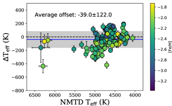
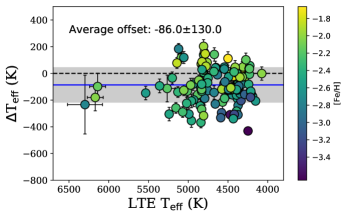
Figure 15: Offsets in effective temperature (spectroscopic $-$ photometric) for the $<$3D$>$, NLTE temperatures (left) and the LTE temperatures (right). The points are color-coded by [Fe/H]. Average offsets are shown with a solid line, while the $1\sigma$ dispersion is shown with a gray band.

A.2 Comparisons of $\log g$ with Gaia DR2 Results

All of the target stars have parallax measurements from Gaia DR2, though the errors are quite large in some cases. These parallax-based distances, combined with $V$ magnitudes and $E(B-V)$ reddenings, give absolute $V$ magnitudes, $M_{V}$. Only parallaxes with errors $<20\%$ are utilized to derive distances (see Bailer-Jones et al. 2018).

Absolute visual magnitudes can also be calculated from the spectroscopic surface gravities. The spectroscopic surface gravities are converted into luminosities and bolometric absolute magnitudes via Equations 3 and 4 of McWilliam & Bernstein (2008). These bolometric magnitudes are then converted into absolute $V$ magnitudes with the bolometric corrections from the Kurucz database, adopting the $T_{\rm{eff}}$, $\log g$, and [Fe/H] interpolation scheme from McWilliam & Bernstein (2008). Figure 16 shows the differences between the spectroscopic (NLTE and LTE) and photometric absolute magnitudes for the subset of stars with sufficiently small errors in the parallax. Both the NLTE and LTE values lead to lower predicted $M_{\rm{V}}$ magnitudes, on average, than predicted by Gaia; in other words, the spectroscopic surface gravities indicate that the stars are slightly brighter than predicted by Gaia, though the average offset and dispersion are smaller when the NLTE corrections are utilized. Although this also may reflect problems with the adopted bolometric corrections, the assumed stellar mass, or the adopted temperature, it may also indicate that additional NLTE corrections are necessary.

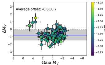
(a) NMTD

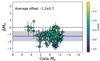
(b) LTE

Figure 16: Offsets in $M_{V}$ (the spectroscopic value derived from $\log g$ and bolometric corrections minus the parallax-based photometric value) for the $<$3D$>$, NLTE temperatures (left) and the LTE temperatures (right). The points are color-coded by [Fe/H]. Average offsets are shown with a solid line, while the $1\sigma$ dispersion is shown with a gray band.

Appendix B LTE Abundances and Atmospheric Parameters for the Target Stars

Table 9 shows the spectroscopic parameters for the target stars if non-LTE corrections are not applied.

Table 9: LTE Atmospheric Parameters: Target Stars

Star	$T_{\rm{eff}}$ (K)	$\log g$	$\xi$ (km/s)	[Fe I/H]		[Fe II/H]
J001236.5$-$181631	4985	2.44	1.49	-2.28±0	-2.42±0.015
J000738.2$-$034551	4663	1.48	2.32	-2.09±0	-2.23±0.031
J002244.9$-$172429	4718	1.11	1.95	-3.38±0	-3.88±0.11
J003052.7$-$100704	4831	1.48	2.2	-2.35±0	-2.42±0.061
J005327.8$-$025317	4370	0.56	1.95	-2.16±0	-2.19±0.036
J005419.7$-$061155	4707	1.03	2.01	-2.32±0	-2.36±0.075
J010727.4$-$052401	5225	3.03	1.43	-2.32±0	-2.51±0.025
J014519.5$-$280058	4582	0.69	2.09	-2.60±0	-2.55±0.049
J015656.3$-$140211	4622	1.09	2.4	-2.08±0	-2.09±0.041
2MJ02134021$-$0005183	6175	4.47	2.6	-1.96±0	-2.17±0.08

Appendix C Systematic Errors

The systematic errors in the abundances are quantified according to the uncertainties in the atmospheric parameters, using the techniques outlined in McWilliam et al. (2013) and Sakari et al. (2017). First, the variances and covariances in the atmospheric parameters were estimated, as shown in Table 10. For the temperature and microturbulence, the uncertainties were determined based on the errors in the slopes of Fe abundance vs. EP and REW, respectively. The uncertainty in gravity was based on the random error in the Fe II abundance, while the uncertainty in the metallicity was based on the random error in the Fe I abundance. The covariances were calculated according to Equation A6 in McWilliam et al. (2013).

Table 10: Variances and Covariances in Atmospheric Parameters for Several Standard Stars

	[Fe/H] $\sim-3$		[Fe/H] $\sim-2.5$				[Fe/H] $\sim-2$
	$\log g\sim 1$		$\log g\sim 1$	$\log g\sim 2$	$\log g\sim 4$		$\log g\sim 1$	$\log g\sim 2$	$\log g\sim 4$
	HE 1523$-$0901		J2038$-$0023	CS 31082-001	BD$-$13 3442		TYC 6535-3183-1	TYC 4924-33-1	TYC 5911-452-1
$\sigma_{T}$	30		25	30	220		55	40	95
$\sigma_{g}$	0.25		0.05	0.15	0.30		0.05	0.20	0.20
$\sigma_{\xi}$	0.16		0.20	0.14	0.35		0.15	0.13	0.28
$\sigma_{\rm{[M/H]}}$	0.02		0.02	0.02	0.02		0.02	0.01	0.02
$\sigma_{T\xi}$	0.08		0.03	0.03	0.10		0.0	2.4	8.07
$\sigma_{Tg}$	0.0		0	0.0	0.0		0.0	0.0	0.0
$\sigma_{g\xi}$	0.08		0.003	0.03	-0.090		0.0	-0.012	-0.015
$\sigma_{T\rm{[M/H]}}$	0		0.32		0.0		0.0	0.48	0.90

The uncertainties in the [Fe/H] and [X/Fe] abundance ratios were then calculated using Equation A1 in Sakari et al. (2017) and Equations A4 and A5 in McWilliam et al. (2013). Table 11 shows the total errors (systematic and random) in the abundance ratios for the six representative standard stars. Only the uncertainties in [X/Fe] are shown; note that the errors in the [X/Fe] ratios are often lower than the errors in the absolute $\log\epsilon$ abundances, since the abundances change together as the atmospheric parameters are varied.

Table 11: Total Errors (Systematic and Random) in the Abundance Ratios for Several Standard Stars

	[Fe/H] $\sim-3$		[Fe/H] $\sim-2.5$				[Fe/H] $\sim-2$
	$\log g\sim 1$		$\log g\sim 1$	$\log g\sim 2$	$\log g\sim 4$		$\log g\sim 1$	$\log g\sim 2$	$\log g\sim 4$
	HE 1523$-$0901		J2038$-$0023	CS 31082-001	BD$-$13 3442		TYC 6535-3183-1	TYC 4924-33-1	TYC 5911-452-1
$\sigma$[Fe I/H]	0.03		0.02	0.02	0.03		0.02	0.02	0.03
$\sigma$[Fe II/H]	0.07		0.08	0.07	0.10		0.10	0.07	0.09
$\sigma$[Li I/Fe]				0.11	0.12		0.09	0.11	0.11
$\sigma$[O I/Fe]							0.12
$\sigma$[Na I/Fe]					0.14		0.16
$\sigma$[Mg I/Fe]	0.01		0.06	0.05	0.12		0.11	0.03	0.04
$\sigma$[Si I/Fe]							0.08	0.12	0.11
$\sigma$[K I/Fe]	0.13		0.11	0.11			0.11	0.10	0.10
$\sigma$[Ca I/Fe]	0.02		0.04	0.03	0.08		0.04	0.02	0.03
$\sigma$[Sc II/Fe]	0.06		0.07	0.07	0.14		0.07	0.04	0.08
$\sigma$[Ti I/Fe]	0.02		0.04	0.04			0.04	0.03	0.05
$\sigma$[Ti II/Fe]	0.05		0.06	0.08	0.07		0.08	0.03	0.09
$\sigma$[V I/Fe]	0.34		0.18	0.11			0.21	0.18
$\sigma$[Cr II/Fe]	0.30		0.18	0.08			0.12	0.08
$\sigma$[Mn I/Fe]	0.08		0.11	0.11			0.05	0.03
$\sigma$[Co I/Fe]	0.40		0.19	0.11			0.10	0.07
$\sigma$[Ni I/Fe]	0.05		0.05	0.03			0.02	0.05
$\sigma$[Cu I/Fe]							0.17
$\sigma$[Zn I/Fe]	0.15		0.11	0.06			0.12	0.15
$\sigma$[Sr II/Fe]	0.13		0.12	0.10	0.24		0.11	0.11	0.18
$\sigma$[Y II/Fe]	0.06		0.09	0.06			0.06	0.08
$\sigma$[Zr II/Fe]	0.09		0.13	0.12			0.14	0.11
$\sigma$[Ba II/Fe]	0.18		0.14	0.06	0.39		0.12	0.05	0.14
$\sigma$[La II/Fe]	0.06		0.08	0.08			0.11	0.02
$\sigma$[Ce II/Fe]	0.05		0.07	0.07			0.06
$\sigma$[Pr II/Fe]	0.09		0.08	0.12			0.06	0.13
$\sigma$[Nd II/Fe]	0.06		0.09	0.06			0.07	0.12
$\sigma$[Sm II/Fe]	0.07		0.13	0.12			0.07
$\sigma$[Eu II/Fe]	0.11		0.12	0.11	0.20		0.18	0.06	0.13
$\sigma$[Dy II/Fe]	0.12			0.12
$\sigma$[Os I/Fe]	0.17			0.12			0.11
$\sigma$[Th II/Fe]			0.12	0.12

Appendix D Equivalent Widths and Line Abundances

Tables 12 and 13 show the EW measurements and abundances for the lines that were determined via EW techniques and spectrum syntheses, respectively.

Table 12: Equivalent Widths

Element	Wavelength	EP	$\log gf$	J0007$-$0345 EW	J0012$-$1816 EW	J0022$-$1724 EW	J0030$-$1007 EW	J0053$-$0253 EW
	(Å)	(eV)		(mÅ)	(mÅ)	(mÅ)	(mÅ)	(mÅ)
Fe I	4383.54	1.48	0.208	—	—	—	—	—
Fe I	4401.44	2.83	-1.650	85.1	39.2	—	—	—
Fe I	4404.75	1.56	-0.147	—	—	—	—	—
Fe I	4408.42	2.20	-1.775	—	49.6	—	—	—
Fe I	4415.12	1.61	-0.621	—	—	—	—	—
Fe I	4430.61	2.22	-1.728	—	50.5	20.8	43.3	—
Fe I	4442.34	2.22	-1.228	—	62.4	—	69.1	—
Fe I	4443.19	2.86	-1.043	76.9	38.4	—	—	87.5
Fe I	4447.72	2.22	-1.339	—	—	—	64.7	—
Fe I	4466.55	2.83	-0.600	—	67.3	26.8	84.8	—

Table 13: Abundances from Synthesized Lines

Element	Wavelength	EP	$\log gf$	J0007$-$0345	J0012$-$1816	J0022$-$1724	J0030$-$1007	J0053$-$0253
	(Å)	(eV)		$\log\epsilon$	$\log\epsilon$	$\log\epsilon$	$\log\epsilon$	$\log\epsilon$
Li I	6707.3	0.000	0.18	—	—	—	—	—
O I	6300.304	0.000	-9.82	—	—	—	—	—
O I	6363.776	0.020	-10.30	—	—	—	—	—
Na I	5682.633	2.101	-0.70	4.25	—	—	—	4.03
Na I	5688.205	2.103	-0.45	4.15	—	—	—	4.08
Na I	5889.951	0.000	0.12	—	—	—	—	—
Na I	5895.924	0.000	-0.18	—	—	—	—	—
Cu I	5105.5	1.388	-1.52	1.43	—	—	—	1.08
Cu I	5782.1	1.641	-1.72	—	—	—	—	—
Zn I	4722.153	4.027	-0.340	2.57	2.68	—	2.69	2.50
Zn I	4810.528	4.075	-0.140	2.60	2.33	—	—	2.45

References

- Abbott et al. (2017) Abbott, B.P., Abbott, R., Abbott, T.D., et al. 2017, PhRvL, 119, 1101
- Abohalima et al. (2017) Abohalima, A. & Frebel, F. 2017, arXiv:1711.04410
- Amarsi et al. (2016) Amarsi, A.M., Lind, K., Asplund, M., Barklem, P.S., & Collet, R. 2016, MNRAS, 463, 1518
- Andrievsky et al. (2007) Andrievsky, S.M., Spite, M., Korotin, S.A., et al. 2007, A&A, 464, 1081
- Arcones & Thielemann (2013) Arcones, A., & Thielemann, F.-K. 2013, Journal of Physics G: Nuclear and Particle Physics, 40, 3201
- Arlandini et al. (1999) Arlandini, C., Käppeler, F., Wisshak, K., Gallino, R., Lugaro, M., Busso, M., Straniero, O. 1999, ApJ, 525, 886
- Asplund et al. (2009) Asplund, M., Grevesse, N., Sauval, J.A., & Scott, P. 2009, ARA&A, 47, 481
- Bailer-Jones et al. (2018) Bailer-Jones, C.A.L., Rybizki, J., Fouesneau, M., Mantelet, G., & Andrae, R. 2018, arXiv:1804.10121
- Barklem et al. (2005) Barklem, P.S., Christlieb, N., Beers, T.C., et al. 2005, A&A, 439, 129
- Barklem (2018) Barklem, P.S. 2018, A&A, 612, A90
- Battaglia et al. (2008) Battaglia, G., Irwin, M., Tolstoy, E., et al. 2008, MNRAS, 383, 183
- Beers et al. (1992) Beers, T.C., Preston, G.W., Shectman, S.A. 1992, AJ, 103, 1987
- Beers & Christlieb (2005) Beers, T.C. & Christlieb, N. 2005, ARA&A, 43, 531
- Beniamini et al. (2016) Beniamini, P., Hotokezaka, K., & Piran, T. 2016, ApJ, 832, 149
- Beniamini et al. (2018) Beniamini, P., Dvorkin, I., & Silk, J. 2018, MNRAS, 478, 1994
- Bergemann & Gehren (2008) Bergemann, M. & Gehren, T., A&A, 492, 823
- Bergemann & Cescutti (2010) Bergemann, M. & Cescutti, G. 2010, A&A, 522, A9
- Bland-Hawthorn et al. (2015) Bland-Hawthorn, J., Sutherland, R., & Webster, D. 2015, ApJ, 807, 154
- Boesgaard et al. (2011) Boesgaard, A.M., Rich, J.A., Levesque, E.M., & Bowler, B.P. 2011, ApJ, 743, 140
- Burris et al. (2000) Burris, D.L., Pilachowski, C.A., Armandroff, T.E., et al. 2000, ApJ, 544, 302
- Caffau et al. (2011) Caffau, E., Bonifacio, P., François, P., et al. 2011, Nature, 477, 67
- Cain et al. (2018) Cain, M., Frebel, A., Gull, M., et al. 2018, arXiv:1807.03734
- Carlsson (1986) Carlsson, M. 1986, Uppsala Astronomical Observatory Reports, 33
- Carlsson (1992) Carlsson, M. 1992, in Cool Stars, Stellar Systems, and the Sun, eds. M. S. Giampapa & J.A. Bookbinder, 26, 499
- Carretta et al. (2009) Carretta, E., Bragaglia, A., Gratton, R., & Lucatello, S. 2009, A&A, 505, 139
- Casagrande et al. (2010) Casagrande, L., Ramírez, I., Meléndez, J., Bessell, M., & Asplund, M. 2010, A&A, 512, 54
- Castelli & Kurucz (2004) Castelli, F. & Kurucz, R. L. 2004, in IAU Symp. 210, Modelling of Stellar Atmospheres, ed. N. Piskunov, W.W. Weiss, & D. F. Gray (San Francisco: ASP), A20
- Cayrel et al. (2001) Cayrel, R., Hill, V., Beers, T.C., et al. 2001, Nature, 409, 691
- Cescutti et al. (2013) Cescutti, G., Chiappini, C., Hirschi, R., Meynet, G., & Frischknecht, U. 2013, A&A, 553, 51
- Cescutti et al. (2015) Cescutti, G., Romano, D., Matteucci, F., Chiappini, C., & Hirschi, R. 2015, A&A, 577, A139
- Chiappini et al. (2011) Chiappini, C., Frischknecht, U., Meynet, G., et al. 2011, Nature, 472, 454
- Chornock et al. (2017) Chornock, R., Berger, E., Kasen, D., et al. 2017, ApJ, 848, L19
- Christlieb et al. (2002) Christlieb, N., Bessell, M.S., Beers, T.C., et al. 2002, Nature, 419, 904
- Christlieb et al. (2004) Christlieb, N., Beers, T.C., Barklem, P.S., et al. 2004, A&A, 428, 1027
- Christlieb et al. (2008) Christlieb, N., Schörck, T., Frebel, A., Beers, T.C., Wisotzki, L., & Reimers, D. 2008, A&A, 484, 721
- Coşkunoǧlu et al. (2011) Coşkunoǧlu, B., Ak, S., Bilir, S. et al. 2011, MNRAS, 412, 1237
- Côté et al. (2017) Côté, B., Fryer, C.L., Belczynski, K., et al. 2017, arXiv:1710.05875
- Cowan & Rose (1977) Cowan, J.J. & Rose, W.K. 1977, ApJ, 212, 149
- Drout et al. (2017) Drout, M.R., Piro, A.L., Shappee, B.J., et al. 2017, Science, 358, 1570
- Eichler et al. (2016) Eichler, M., Arcones, A., Käppeli, R., et al. 2016, JPhCS, 665, 2054
- El-Badry et al. (2018) El-Badry, K., Bland-Hawthorn, J., Wetzel, A., et al. 2018, MNRAS, 480, 652
- Ezzeddine et al. (2016) Ezzeddine, R., Merle, T., & Plez, B. 2016, Astronomische Nachrichten, 337, 850
- Ezzeddine et al. (2017) Ezzeddine, R., Frebel, A., & Plez, B. 2017, ApJ, 847, 142
- Frebel et al. (2005) Frebel, A., Aoki, W., Christlieb, N., et al. 2005, Nature, 434, 871
- Frebel et al. (2007) Frebel, A., Christlieb, N., Norris, J.E., Thom, C., Beers, T.C., & Rhee, J. 2007, ApJ, 660, 117
- Frebel et al. (2013) Frebel, A., Casey, A.R., Jacobson, H.R., & Yu, Q. 2013, ApJ, 769, 57
- Frebel & Norris (2015) Frebel, A. & Norris, J.E. 2015, ARA&A, 53, 631
- Frebel (2018) Frebel, A. 2018, arXiv:1806.08955
- Frischknecht et al. (2012) Frischknecht, U., Hirschi, R., & Thielemann, F.-K. 2012, A&A, 538, 2
- Frischknecht et al. (2016) Frischknecht, U., Hirschi, R., Pignatari, M., et al. 2016, MNRAS, 456, 1803
- Fulbright et al. (2006) Fulbright, J.P., McWilliam, A., & Rich, R.M. 2006, ApJ, 636, 821
- Fulbright et al. (2007) Fulbright, J.P., McWilliam, A., & Rich, R.M. 2007, ApJ, 661, 1152
- Gaia Collaboration et al. (2016) Gaia Collaboration, Prusti, T., de Bruijne, J.H.J., et a. 2016, A&A, 595, A1
- Gaia Collaboration et al. (2018) Gaia Collaboration, Brown, A.G.A., Vallenari, A., Prusti, T., de Bruijne, J.H.J., Babusiaux, C., & Bailer-Jones, C.A.L. 2018, A&A, arXiv:1804.09365
- Gratton et al. (2004) Gratton, R., Sneden, C., & Carretta, E. 2004, ARA&A, 42, 385
- Gull et al. (2018) Gull, M., Frebel, A., Cain, M.G., et al. 2018, arXiv:1806.00645
- Gustafsson et al. (2008) Gustafsson, B., Edvardsson, B., Eriksson, K., Jørgensen, U.G., Nordlund, Å., & Plez, B. 2008, A&A, 486, 951
- Hampel et al. (2016) Hampel, M., Stancliffe, R.J., Lugaro, M., & Meyer, B.S. 2016, ApJ, 831, 171
- Hansen et al. (2013) Hansen, C.J., Bergemann, M., Cescutti, G., François, P., Arcones, A., Karakas, A.I., Lind, K., and Chiappini, C. 2013, A&A, 551, A57
- Hansen et al. (2015) Hansen, T.T., Andersen, J., Nordström, B., Beers, T.C., Yoon, J., & Buchhave, L.A. 2015, A&A, 583, 49
- Hansen et al. (2017) Hansen, T.T., Simon, J.D., Marshall, J.L., et al. 2017, ApJ, 838, 44
- Hansen et al. (2018) Hansen, T.T., Holmbeck, E.M., Beers, T.C., et al. 2018, ApJ, 858, 92
- Herwig et al. (2011) Herwig, F., Pignatari, M., Woodward, P.R., et al. 2011, ApJ, 727, 89
- Hill et al. (2002) Hill, V., Plez, B., Cayrel, R., et al. 2002, A&A, 387, 560
- Hill et al. (2017) Hill, V., Christlieb, N., & Beers, T. C., et al. 2017, A&A, 607, 91
- Hinkle et al. (2003) Hinkle, K., Wallace, L., Livingston, W., Ayres, T., Harmer, D., & Valenti, J. 2003, in The Future of Cool-Star Astrophysics: 12th Cambridge Workshop on Cool Stars, Stellar Systems, and the Sun (2001 July 30 - August 3), eds. A. Brown, G.M. Harper, and T.R. Ayres, (University of Colorado), 851
- Hollek et al. (2011) Hollek, J.K., Frebel, A., Roederer, I.U., Sneden, C., Shetrone, M., Beers, T.C., Kang, S.-J., Thom, C. 2011, ApJ, 742, 54
- Hollek et al. (2015) Hollek, J.K., Frebel, A., Placco, V.M., Karakas, A.I., Shetrone, M., Sneden, C., & Christlieb, N. 2015, ApJ, 814, 121
- Holmbeck et al. (2018a) Holmbeck, E.M., Beers, T.C., Roederer, I.U., et al. 2018a, ApJ, 859, 24
- Holmbeck et al. (2018b) Holmbeck, E.M., Surman, R., Sprouse, T.M., Mumpower, M.R., Vassh, N., Beers, T.C., & Kawano, T. 2018, arXiv:1807.06662
- Honda et al. (2006) Honda, S., Aoki, W., Ishimaru, Y., Wanajo, S., & Ryan, S.G. 2006, ApJ, 643, 1180
- Ito et al. (2009) Ito, H., Aoki, W., Honda, S., & Beers, T.C. 2009, ApJ, 698, L37
- Ji et al. (2016) Ji, A.P., Frebel, A., Simon, J.D., & Chiti, A. 2016, ApJ, 830, 93
- Ji & Frebel (2018) Ji, A.P. & Frebel, A. 2018, ApJ, 856, 138
- Keller et al. (2007) Keller, S.C., Schmidt, B.P., Bessell, M.S., et al. 2007, PASA, 24, 1
- Keller et al. (2014) Keller, S.C., Bessell, M.S., Frebel, A., et al. 2014, Nature, 506, 463
- Koch & McWilliam (2008) Koch, A. & McWilliam, A. 2008, AJ, 135, 1551
- Koppelman et al. (2018) Koppleman, H., Helmi, A., & Veljanoski, J. 2018, ApJ, 860, L11
- Kordopatis et al. (2013a) Kordopatis, G., Gilmore, G., Steinmetz, M., et al. 2013a, AJ, 146, 134
- Kordopatis et al. (2013b) Kordopatis, G., Gilmore, G., Wyse, R.F.G., et al. 2013b, MNRAS, 436, 3231
- Kraft & Ivans (2003) Kraft, R.P, & Ivans, I.I. 2003, PASP, 115, 143
- Kunder et al. (2017) Kunder, A., Kordopatis, G., Steinmetz, M., et al. 2017, AJ, 153, 75
- Lattimer & Schramm (1974) Lattimer, J. & Schramm, D. 1974, ApJ, 192, L145
- Li et al. (2015) Li, H.-N., Zhao, G., Christlieb, N., et al. 2015, ApJ, 798, 110
- Lind et al. (2011) Lind, K., Asplund, M., Barklem, P.S., & Belyaev, A.K. 2011, A&A, 528, A103
- Lind et al. (2012) Lind, K., Bergemann, M., & Asplund, M. 2012, MNRAS, 427, 50
- Lippuner et al. (2017) Lippuner, J., Fernández, R., Roberts, L.F., Foucart, F., Kasen, D., Metzger, B.D., & Ott, C.D. 2017, MNRAS, 472, 904
- Macias & Ramirez-Ruiz (2016) Macias, P. & Ramirez-Ruiz, E. 2016, arXiv:1609.04826
- Martell et al. (2016) Martell, S.L., Shetrone, M.D., Lucatello, S., et al. 2016, ApJ, 825, 146
- Mashonkina et al. (2014) Mashonkina, L., Christlieb, N., & Eriksson, K. 2014, A&A, 569, A43
- Matijevic̆ et al. (2017) Matijevic̆, G., Chiappini, C., Grebel, E.K., et al. 2017, A&A, 603, 19
- McCall (2004) McCall, M.L. 2004, AJ, 128, 2144
- McWilliam et al. (1995) McWilliam, A., Preston, G.W., Sneden, C., & Searle, L. 1995b, AJ, 109, 2757
- McWilliam & Bernstein (2008) McWilliam, A. & Bernstein, R. 2008, ApJ, 684, 326
- McWilliam et al. (2013) McWilliam, A., Wallerstein, G., & Mottini, M. 2013, ApJ, 778, 149
- Mösta et al. (2017) Mösta, P., Roberts, L.F., Halevi, G., Ott, C.D., Lippuner, J., Haas, R., & Schnetter, E. 2017, arXiv:1712.09370
- Nissen & Schuster (2010) Nissen, P.E. & Schuster, W.J. 2010, A&A, 511, 10
- Norris et al. (2007) Norris, J.E., Christlieb, N., Korn, A.J., et al. 2007, ApJ, 670, 774
- O’Malley et al. (2017) O’Malley, E.M., McWilliam, A., Chaboyer, B., & Thompson, I. 2017, ApJ, 838, 90
- Pietrinferni et al. (2004) Pietrinferni, A., Cassisi, S., Salaris, M. & Castelli, F. 2004, ApJ, 612, 168
- Placco et al. (2014a) Placco, V.M., Beers, T.C., Roederer, I.U., et al. 2014a, ApJ, 790, 34
- Placco et al. (2014b) Placco, V.M., Frebel, A., Beers, T.C., & Stancliffe, R.J. 2014b, ApJ, 797, 21
- Placco et al. (2015) Placco, V.M., Frebel, A., Lee, Y.S., et al. 2015, ApJ, 809, 136
- Placco et al. (2017) Placco, V.M., Holmbeck, E.M., Frebel, A., et al. 2017, ApJ, 844, 18
- Placco et al. (2018) Placco, V.M., Beers, T.C., Santucci, R.M., et al. 2018, ApJ, 155, 256
- Ramírez & Meléndez (2005) Ramírez, I. & Meléndez, J. 2005, ApJ, 626, 465
- Reddy et al. (2006) Reddy, B.E., Lambert, D.L., & Prieto, C.A. 2006, MNRAS, 367, 1329
- Reggiani et al. (2016) Reggiani, H., Meléndez, J., Yong, D., Ramírez, I., & Asplund, M. 2016, A&A, 586, 67
- Reggiani et al. (2017) Reggiani, H., Meléndez, J., Kobayashi, C., Karakas, A., & Placco, V. 2017, A&A, 608, 46
- Roederer et al. (2010) Roederer, I.U., Cowan, J.J., Karakas, A.I., et al. 2010, ApJ, 724, 975
- Roederer et al. (2014a) Roederer, I.U., Preston, G.W., Thompson, I.B., Shectman, S.A., Sneden, C., Burley, G.S., & Kelson, D.D. 2014a, AJ, 147, 136
- Roederer et al. (2014b) Roederer, I.U., Cowan, J.J., Preston, G.W., Shectman, S.A., Sneden, C., & Thompson, I.B. 2014b, MNRAS, 445, 2946
- Roederer et al. (2016) Roederer, I.U., Mateo, M., Bailey, J.I., et al. 2016, AJ, 151, 82
- Roederer et al. (2018a) Roederer, I.U., Hattori, K., & Valluri, M. 2018a, AJ, in press, arXiv:1808.09467
- Roederer et al. (2018b) Roederer, I.U., Sakari, C.M., Placco, V.M., Beers, T.C., Ezzeddine, R., Frebel, A., & Hansen, T.T. 2018b, ApJ, in press, arXiv:1808.09469
- Rosswog et al. (2014) Rosswog, S., Korobkin, O., Arcones, A., Thielemann, F.-K., Piran, T. 2014, MNRAS, 439, 744
- Ruchti et al. (2011) Ruchti, G.R., Fulbright, J.P., Wyse, R.F.G., et al. 2011, ApJ, 737, 9
- Ruchti et al. (2013) Ruchti, G.R., Bergemann, M., Serenelli, A., Casagrande, L., & Lind, K. 2013, MNRAS, 429, 126
- Sakari et al. (2017) Sakari, C.M., McWilliam, A., & Wallerstein, G. 2017, MNRAS, 467, 1112
- Sakari et al. (2018) Sakari, C.M., Placco, V.M., Hansen, T., et al. 2018, ApJ, 854, L20
- Schatz et al. (2002) Schatz, H., Toenjes, R., Pfeiffer, B., Beers, T.C., Cowan, J.J., Hill, V., & Kratz, K.-L. 2002, ApJ, 579, 626
- Schiavon et al. (2017) Schiavon, R.P., Zamora, O., Carrera, R., et al. 2017, MNRAS, 465, 501
- Schlafly & Finkbeiner (2011) Schlafly, E.F., & Finkbeiner, D.P. 2011, ApJ, 737, 103
- Schlaufman & Casey (2014) Schlaufman, K.C. & Casey, A.R. 2014, ApJ, 797, 13
- Shappee et al. (2017) Shappee, B.J., Simon, J.D., Drout, M.R., et al. 2017, Science, 358, 1574
- Shi et al. (2018) Shi, J.R., Yan, H.L., Zhou, Z.M., & Zhao, G. 2018, arXiv:1806.02225
- Short & Hauschildt (2006) Short, C.I. & Hauschildt, P.H. 2006, ApJ, 641, 494
- Siqueira Mello et al. (2013) Siqueira Mello, C., Spite, M., Barbuy, B. 2013, A&A, 550, 122
- Siqueira Mello et al. (2014) Siqueira Mello, C., Hill, V., Barbuy, B., et al. 2014, A&A, 565, 93
- Skrutskie et al. (2006) Skrutskie, M.F., Cutri, R.M., Stiening, R., et al. 2006, AJ, 131, 1163
- Sneden (1973) Sneden, C. 1973, ApJ, 184, 839
- Sneden et al. (1996) Sneden, C., McWilliam, A., Preston, G.W., Cowan, J.J., Burris, D.L., & Armosky, B.J. 1996, ApJ, 467, 819
- Sneden et al. (2008) Sneden, C., Cowan, J.J., & Gallino, R. 2008, ARA&A, 46, 241
- Sneden et al. (2009) Sneden, C., Lawler, J.E., Cowan, J.J., Ivans, I.I., & Den Hartog, E.A. 2009, ApJS, 182, 80
- Sobeck et al. (2011) Sobeck, J. S., Kraft, R. P., Sneden, C., et al. 2011, AJ, 141, 175
- Spite et al. (2018) Spite, F., Spite, M., Barbuy, B., Bonifacio, P., Caffau, E., & François, P. 2018, A&A, 611, A30
- Starkenburg et al. (2010) Starkenburg, E., Hill, V., Tolstoy, E., et al. 2010, A&A, 513, 34
- Starkenburg et al. (2017) Starkenburg, E., Oman, K.A., Navarro, J.F., et al. 2017, MNRAS, 465, 2212
- Steinmetz et al. (2006) Steinmetz, M., Zwitter, T., Siebert, A., et al. 2006, AJ, 132, 1645
- Stetson & Pancino (2008) Stetson, P.B. & Pancino, E. 2008, PASP, 120, 1332
- Surman et al. (2017) Surman, R., Mumpower, M., & McLaughlin, G. 2017, Proc. of the 14th International Symposium on Nuclei in the Cosmos, ed. Kubono, S., Kajino, T., Nishimura, S., Isobe, T., Nagataki, S. Shima, T., & Takeda, Y.
- Thanathibodee (2016) Thanathibodee, T. 2016, “Chemical abundance analysis of HE 2324-0215, an r-process-enhanced metal-poor star,” Massachusetts Institute of Technology
- Tsujimoto & Nishimura (2015) Tsujimoto, T. & Nishimura, N. 2015, ApJ, 811, L10
- Tsujimoto et al. (2017) Tsujimoto, T., Matsuno, T., Aoki, W., Ishigaki, M.N., & Shigeyama, T. 2017, ApJ, 850, L12
- van Leeuwen (2007) van Leeuwen, F. 2007, A&A, 474, 653
- Venn et al. (2004) Venn, K.A., Irwin, M., Shetrone, M.D., et al. 2004, AJ, 128, 1177
- Winteler et al. (2012) Winteler, C., Käppeli, R., Perego, A., Arcones, A., Vasset, N., Nishimura, N., Liebendörfer, M., & Thielemann, F.-K. 2012, ApJ, 750, L22
- Xu et al. (2007) Xu, H.L., Svanberg, S., Quinet, P., Palmeri, P., & Biémont, É. 2007, JQSRT, 104, 52