Lattice Boltzmann model with self-tuning equation of state for coupled thermo-hydrodynamic flows
Abstract
A novel lattice Boltzmann (LB) model with self-tuning equation of state (EOS) is developed in this work for simulating coupled thermo-hydrodynamic flows. The velocity field is solved by the recently developed multiple-relaxation-time (MRT) LB equation for density distribution function (DF), by which a self-tuning EOS can be recovered. As to the temperature field, a novel MRT LB equation for total energy DF is directly developed at the discrete level. By introducing a density-DF-related term into this LB equation and devising the equilibrium moment function for total energy DF, the viscous dissipation and compression work are consistently considered, and by modifying the collision matrix, the targeted energy conservation equation is recovered without deviation term. The full coupling of thermo-hydrodynamic effects is achieved via the self-tuning EOS and the viscous dissipation and compression work. The present LB model is developed on the basis of the standard lattice, and various EOSs can be adopted in real applications. Moreover, both the Prandtl number and specific heat ratio can be arbitrarily adjusted. Furthermore, boundary condition treatment is also proposed on the basis of the judicious decomposition of DF into its equilibrium, force (source), and nonequilibrium parts. The local conservation of mass, momentum, and energy can be strictly satisfied at the boundary node. Numerical simulations of thermal Poiseuille and Couette flows are carried out with three different EOSs, and the numerical results are in good agreement with the analytical solutions. Then, natural convection in a square cavity with a large temperature difference is simulated for the Rayleigh number from up to . Good agreement between the present and previous numerical results is observed, which further validates the present LB model for coupled thermo-hydrodynamic flows.
keywords:
lattice Boltzmann model , coupled thermo-hydrodynamic flows , self-tuning equation of state , viscous dissipation and compression work , boundary condition treatment , standard lattice1 Introduction
The lattice Boltzmann (LB) method has developed into an attractive numerical method over the past three decades for simulating complex fluid flows [1, 2, 3] and solving various partial differential equations [4, 5, 6]. Historically, the LB method originates from the lattice gas automata (LGA) to eliminate the statistical noise [7], and thus it inherits some distinguishing features from LGA, such as the simple algorithm (local collision and linear streaming) and the easy incorporation of microscopic interactions [8, 9]. Afterward, it is found that the classical LB model for hydrodynamic flows can be derived from the Boltzmann-BGK equation via systematic discretization [10, 11], and then various LB models for multiphase flows [12, 13] and thermo-hydrodynamic flows (i.e., thermal fluid flows) [14, 15] have been established from the kinetic models in an a priori manner.
Since most hydrodynamic flows involve some forms of thermal effects, thermo-hydrodynamic flows are extensively encountered in nature and engineering, and the LB method for simulating thermo-hydrodynamic flows has attracted continuous attention since the early 1990s [14, 15, 16, 17, 18, 19, 20, 21, 22, 23, 24]. However, it remains open-ended though the LB method has achieved great success in simulating isothermal fluid flows [25, 26]. Generally, the existing LB models for thermo-hydrodynamic flows can be categorized into three major groups: the multispeed approach [18, 19], the double-distribution-function (DDF) approach [14, 15, 16], and the hybrid approach [20, 21]. The multispeed approach uses a single distribution function (DF) to describe the mass, momentum, and energy conservation laws, and thus it requires more discrete velocities than the standard lattice (i.e., it requires the multispeed lattice). By definition, the DDF approach consists of double DFs, with one DF for the mass and momentum conservation laws and the other DF for the energy conservation law. In the hybrid approach, the mass and momentum conservation laws are described by one DF, while the energy conservation law is described by a macroscopic governing equation that is solved via the conventional computational fluid dynamics methods. Severe numerical instability [20] and complexity of boundary condition treatment [27] are usually encountered in the multispeed approach. As to the hybrid approach, it acts as a compromised solution that deviates from the mesoscopic LB method [20], and the viscous dissipation is usually ignored in this approach [28, 29]. On the contrary, the DDF approach, free of the above drawbacks, is most widely studied and adopted in real applications.
Most of the existing DDF LB models for thermo-hydrodynamic flows are inherently a decoupling model, which means that the recovered equation of state (EOS) is a decoupling EOS ( is the gas constant and is the reference temperature), where the pressure is not directly related to the temperature. Consequently, these LB models are restricted to the thermo-hydrodynamic flows under the Boussinesq approximation (i.e., the decoupling thermo-hydrodynamic flows). Based on the DDF kinetic model constructed by Guo et al. [15], and by applying the discretization of velocity space presented by Shan et al. [30] that can lead to the temperature-independent discrete velocities, Hung and Yang [31] proposed a DDF LB model aimed at recovering the ideal-gas EOS . However, the deviation in the third-order moment of the equilibrium distribution function (EDF) for density due to the constraint of standard lattice, as previously identified by Prasianakis and Karlin [32], is not considered in Hung and Yang’s model, and meanwhile, an error also exists in their derived EDF for total energy. In 2012, by introducing the correction term for the third-order moment of the EDF for density and deriving the correct EDF for total energy, Li et al. [33] developed a DDF LB model for simulating coupled thermo-hydrodynamic flows. The ideal-gas EOS can be recovered by Li et al.’s model, and the simulation of natural convection with a large temperature difference is reported [33]. Following the similar way, Feng et al. [34] proposed three-dimensional DDF LB models. A correction term for the second-order moment of the EDF for total energy is further introduced by Feng et al. [34] to enhance the numerical stability of the LB equation for total energy DF. Recently, the cascaded collision scheme is employed in the LB equation for density DF to enhance the numerical stability by Fei and Luo [35], while the single-relaxation-time (SRT) collision scheme is still used in the LB equation for total energy DF.
It is worth pointing out that the ideal-gas EOS is recovered by the above DDF LB models [31, 33, 34, 35], which indicates that these models are only applicable to the coupled thermo-hydrodynamic flows of ideal gases. Moreover, in these models, the LB equation for total energy DF is complicated due to the consideration of the viscous dissipation and compression work, and thus it is difficult to employ the multiple-relaxation-time (MRT) or cascaded collision schemes in this LB equation to enhance the numerical stability although the MRT and cascaded collision schemes have been employed in the LB equation for density DF [33, 35]. Most recently, we developed an LB model with self-tuning EOS for multiphase flows [36]. Since the recovered EOS can be self-tuned via a built-in variable, this model serves as a good and distinct starting point for developing a novel LB model for coupled thermo-hydrodynamic flows, which is the main objective of the present work. To be specific, a novel MRT LB equation for solving the energy conservation equation, with considering the viscous dissipation and compression work, is developed. Furthermore, boundary condition treatment for simulating coupled thermo-hydrodynamic flows is also proposed on the basis of the judicious decomposition of DF into three parts rather than two. The remainder of the present paper is organized as follows. In Section 2, a novel LB model for coupled thermo-hydrodynamic flows is developed. In Section 3, boundary condition treatment is proposed. Numerical validations of the present LB model are carried out in Section 4, and a brief conclusion is drawn in Section 5.
2 Lattice Boltzmann model
The present LB model for coupled thermo-hydrodynamic flows is developed on the basis of the recent LB model with self-tuning EOS for multiphase flows. Double DFs are involved: one is the density DF used to solve the velocity field (i.e., the mass-momentum conservation equations), and the other is the total energy DF used to solve the temperature field (i.e., the energy conservation equation). The full coupling of thermo-hydrodynamic effects is achieved via the self-tuning EOS recovered by the LB equation for density DF and the viscous dissipation and compression work considered in the LB equation for total energy DF. Both the LB equations for density and total energy DFs are based on the standard lattice. For the sake of simplicity and clarity, the two-dimensional model will be developed here, and its extension to three-dimensional model is straightforward. The standard two-dimensional nine-velocity (D2Q9) lattice is given as [37]
| (1) |
where the lattice speed with and being the lattice spacing and time step, respectively.
2.1 LB equation for density DF
The recently developed LB equation for density DF that can recover a self-tuning EOS is briefly introduced here for self-completeness. The MRT LB equation for density DF can be expressed as [36]
| (2a) | |||
| (2b) |
where Eq. (2a) is the streaming process executed in velocity space and Eq. (2b) is the collision process executed in moment space at position and time . The moment of density DF in Eq. (2b) is given as . Here, is the dimensionless transformation matrix [38]
| (3) |
and denotes the vector . The post-collision density DF in Eq. (2a) is obtained via the inverse transformation , and the post-collision moment is computed by Eq. (2b). The last three terms on the right-hand side (RHS) of Eq. (2b) are the correction terms aimed at eliminating the additional cubic terms of velocity in the recovered momentum conservation equation [39], where denotes the recovered EOS by the LB equation. The macroscopic density and velocity are defined as
| (4) |
where is the force term. In the recent LB model for multiphase flows [36], is the total force due to the long-range molecular interaction, while in the present LB model for coupled thermo-hydrodynamic flows, is simply an external force, such as the gravity force.
In Eq. (2b), the equilibrium moment function for density DF is given as [36]
| (5) |
where and is the built-in variable aimed at achieving a self-tuning EOS. The coefficients and are set to and , respectively, while the coefficients and are determined by Eq. (8). The discrete force term in moment space is given as
| (6) |
where , and the square bracket and its subscript denote permutation and tensor index, respectively. For example, . To correctly recover the Newtonian viscous stress tensor, the collision matrix in moment space is modified as follows [36]
| (7) |
where , and , , and are the coefficients. Through the Chapman-Enskog analysis, the coefficients in and should satisfy the following relations
| (8) |
where is related to the bulk viscosity.
In Eq. (2b), the last three terms, together with the high-order terms of velocity in and , are introduced to eliminate the additional cubic terms of velocity [39], which are not considered in the previous DDF LB models for coupled thermo-hydrodynamic flows. The correction matrix is a matrix and it is set as [36]
| (9a) | |||
| where the nonzero elements can be determined via the Chapman-Enskog analysis as follows | |||
| (9b) | |||
The correction matrix is set as [36]
| (10a) | |||
| whose element is a vector implying that the dimensions of are . The nonzero elements in can also be determined via the Chapman-Enskog analysis as follows | |||
| (10b) | |||
Similarly to , the correction matrix is a matrix and it is set as [36]
| (11a) | |||
| where the nonzero elements are given as | |||
| (11b) | |||
Here, we would like to point out that for the coupled thermo-hydrodynamic flows under the low Mach number condition, these correction terms for the additional cubic terms of velocity can be simply ignored. However, they are kept in the present work for the sake of theoretical completeness and computational accuracy.
Through the Chapman-Enskog analysis, the following mass-momentum conservation equations can be recovered [36]
| (12) |
where and are the recovered EOS and viscous stress tensor
| (13) |
where the lattice sound speed , the kinematic viscosity , and the bulk viscosity . As seen in Eq. (13), the recovered EOS can be arbitrarily tuned via the built-in variable .
2.2 LB equation for total energy DF
Since the EOS recovered by the above LB equation for solving the velocity field can be self-tuned, we are now well equipped to simulate coupled thermo-hydrodynamic flows. The remaining task is to develop an LB equation for solving the temperature field, in which the viscous dissipation and compression work are consistently considered.
2.2.1 Energy conservation equation
The collision term of an LB equation conserves macroscopic quantity, and the recovered macroscopic conservation equation for this quantity usually has a conservative form (see Eq. (13) as an example). On the basis of this principle, the total energy conservation equation, in which the viscous dissipation and compression work are expressed as , is a better and more natural starting point for directly developing an LB equation at the discrete level than the internal energy conservation equation, in which the viscous dissipation and compression work are expressed as . Here, is the pressure determined by the adopted EOS. To facilitate the development of an LB equation, the total energy conservation equation is reformulated as
| (14) |
where is the total energy, is the total enthalpy, is the temperature that can be determined by the internal energy () and density , is the heat conductivity, and is the source term. In Eq. (14), the viscous dissipation combines with the conduction term to constitute the term , and the compression work combines with the convection term to constitute the term . Meanwhile, we can also combine the work done by force and the source term to constitute an equivalent source term . Thus, Eq. (14) can be viewed as a general convection-diffusion equation with source term. Here, we would like to point out that the above reformulation is consistent with the Chapman-Enskog analysis, which means that the two terms combined together are of the same order.
2.2.2 Viscous stress tensor
To consider the viscous dissipation in the LB equation for total energy DF, we first recall the recovery of viscous stress tensor by the above LB equation for density DF. On the basis of the Chapman-Enskog analysis, the viscous stress tensor is of order and can be expressed as [36]
| (15) |
where is the small expansion parameter in the Chapman-Enskog analysis and is
| (16) |
where and are the terms of and in their Chapman-Enskog expansions and , respectively. Here, it is worth pointing out that the post-collision moment is kept in Eq. (16) rather than being substituted by Eq. (2b). As a consequence, the post-collision moment , which is computed in the collision process of density DF, can be directly utilized to consider the viscous dissipation in the LB equation for total energy DF (see C). Moreover, from the Chapman-Enskog analysis of the LB equation for density DF, we can easily know that the terms of and satisfy
| (17) |
2.2.3 LB equation
For the energy conservation equation given by Eq. (14), the total energy DF is introduced here, and the MRT LB equation for is devised as
| (18a) | |||
| (18b) |
where Eqs. (18a) and (18b) represent the streaming process in velocity space and the collision process in moment space, respectively. The moment of total energy DF in Eq. (18b) is given as , the post-collision total energy DF in Eq. (18a) is obtained via , and the post-collision moment is computed by Eq. (18b). Here, the dimensionless transformation matrix is also given by Eq. (3). On the RHS of Eq. (18b), the last density-DF-related term is introduced to consider the viscous dissipation, in which is a matrix that will be discussed and determined later. By definition, the macroscopic total energy is given as
| (19) |
where is the equivalent source term. Then, the total enthalpy and the temperature can be determined via the thermodynamic relations and (a function of internal energy and density ), respectively. In the present work, a simple relation , though it strictly holds only for the ideal gases, is adopted for the sake of simplicity, and more general or empirical relations can be adopted as required by specific applications. Here, is the specific heat at constant volume.
To recover the targeted energy conservation equation, as well as inspired by the ideas of our previous works on solid-liquid phase change [40, 3], the equilibrium moment function for total energy DF is devised as
| (20) |
where and are the reference density and the reference specific heat at constant pressure, respectively, and and are the coefficients related to the heat conductivity. Similarly to , the discrete source term in moment space is devised as
| (21) |
To avoid the deviation term caused by the convection term recovered at the order of in the diffusion term recovered at the order of , the collision matrix in moment space is modified as follows [41]
| (22) |
where .
Since the viscous stress tensor is only related to , , and (see Eq. (15)), the matrix in the density-DF-related term, which is introduced in Eq. (18b) to consider the viscous dissipation, is set as follows
| (23) |
where and for , , and . Through the Chapman-Enskog analysis (see A), the nonzero elements in can be determined as follows
| (24) |
Then, the following macroscopic conservation equation can be recovered
| (25) |
Compared with Eq. (14), the heat conductivity is given as . It can be seen from Eq. (25) that the viscous dissipation and compression work are correctly considered.
Before proceeding further, some discussion on the present LB model for coupled thermo-hydrodynamic flows is in order. First, the MRT collision scheme is employed in both the LB equations for density and total energy DFs, and the collision matrix in moment space is modified to be a nondiagonal matrix rather than being set as the conventional diagonal matrix. Second, the Prandtl number can be arbitrarily adjusted. Here, is the specific heat at constant pressure, and is the dynamic viscosity. Third, the specific heat ratio can also be arbitrarily adjusted. Note that depends on the adopted EOS, and holds only for the ideal-gas EOS. Lastly, and most importantly, an arbitrary EOS (including the nonideal-gas EOS) can be prescribed, and the built-in variable is inversely calculated via with .
3 Boundary condition treatment
In real applications, the boundary conditions are usually given in terms of the macroscopic variables, and thus additional treatment is required to obtain the mesoscopic DFs at the boundary node. In this section, we propose the boundary condition treatment for simulating coupled thermo-hydrodynamic flows.
3.1 Macroscopic variables
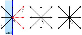
For the velocity field, the nonslip velocity boundary condition is considered and the velocity on the boundary is directly specified. Due to the full coupling of thermo-hydrodynamic effects, the density may significantly vary near the boundary and also has a direct effect on the heat transfer process. Thus, it is important to ensure the mass conservation at the boundary node for simulating coupled thermo-hydrodynamic flows. In the present boundary condition treatment, the boundary node is exactly placed on the wall boundary, as shown in Fig. 1. The post-collision density DF hitting the wall (i.e., streaming out of the computational domain) reverses its direction as follows
| (26) |
where means , and the subscript “temp” implies that the density DF is temporary. After this “bounce-back” process, all the unknown density DFs at and due to the absence of adjacent nodes are now obtained. Then, the density can be computed via definition as usual (i.e., ). Note that the velocity is directly specified. Obviously, the local conservation of mass can be strictly satisfied at the boundary node.
As for the temperature field, the Dirichlet boundary condition with specified temperature and the Neumann boundary condition with zero heat flux (i.e., the adiabatic boundary condition) are considered. For the Dirichlet boundary condition, since the temperature is directly specified, all the involved macroscopic variables, such as the total energy , the pressure , and the total enthalpy , can be determined via the corresponding thermodynamic relations. For the Neumann boundary condition with zero heat flux, the post-collision total energy DF hitting the wall reverses its direction as follows
| (27) |
and thus all the unknown total enthalpy DFs at and due to the absence of adjacent nodes are temporarily obtained. Then, the total energy can be computed via definition as usual (i.e., ), and all the involved macroscopic variables, such as the temperature , the pressure , and the total enthalpy , can be determined via the corresponding thermodynamic relations.
3.2 Density and total energy DFs
At the boundary node, the unknown density and total energy DFs obtained via Eqs. (26) and (27) are only used to compute the macroscopic density and total energy. In the present boundary condition treatment, all the known and unknown DFs at the boundary node will be updated to make sure that the defining equations of density, velocity, and total energy (i.e., Eqs. (4) and (19)) exactly hold at the boundary node. For this purpose, we decompose the moment of DF (the same as the DF) into its equilibrium, force (source), and nonequilibrium parts, i.e.,
| (28a) | |||
| (28b) |
Note that the present nonequilibrium part () in Eq. (28) is different from the previous nonequilibrium part defined as () [42] when the force (source) term exists. Since the equilibrium parts ( and ) and the force (source) parts ( and ) are determined by the macroscopic variables, and can be directly computed. As to the nonequilibrium parts ( and ) at and , extrapolations are employed following the idea of the nonequilibrium-extrapolation approach [43, 44]. However, instead of simply extrapolating and , we introduce the following terms
| (29a) | |||
| (29b) |
where is the identity matrix; and then the first- and second-order nonequilibrium extrapolations are given as
| (30a) | |||
| (30b) |
where and denote the nearest and next-nearest fluid nodes in the normal direction, as shown in Fig. 1. Based on our numerical tests, the first-order extrapolation has better stability but lower accuracy than the second-order extrapolation. Note that although the present collision matrices and are nondiagonal, and in Eq. (29) are still invertible, and their inverse matrices are given in B. Therefore, Eq. (30) is compatible and can be easily implemented due to the special forms of and . Moreover, different from the previous nonequilibrium-extrapolation approach [43, 44, 15], the present boundary condition treatment is applicable to the situation when the dynamic viscosity and thermal conductivity significantly vary with temperature and hence with space because the collision matrices are considered in the present extrapolations of nonequilibrium parts.
4 Validations and discussions
In this section, simulations of thermal Poiseuille and Couette flows are first carried out to validate the present LB model with self-tuning EOS for coupled thermo-hydrodynamic flows. Three different EOSs, including the decoupling EOS, the ideal-gas EOS, and the Carnahan-Starling EOS for rigid-sphere fluids [45], are adopted, which are given in order as follows
| (31a) | |||
| (31b) | |||
| (31c) |
where is the compressibility factor with the coefficient set to here. Then, the present LB model is applied to the simulation of natural convection in a square cavity with a large temperature difference. The ideal-gas EOS is adopted and the Rayleigh number varies from up to . In the following simulations, , , and are chosen. The relaxation parameters in satisfy , , and [46], and the relaxation parameters in satisfy , , , and [3]. Meanwhile, the ratio of bulk to kinematic viscosity is fixed at unless otherwise stated.
4.1 Thermal Poiseuille flow
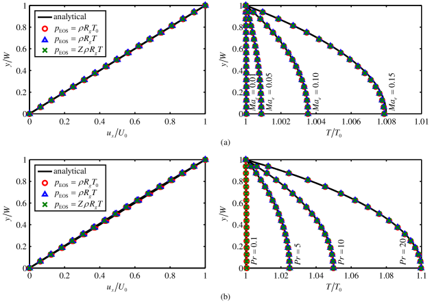
The thermal Poiseuille flow, driven by a constant force between two parallel walls, is first simulated. Both the lower and upper walls are at rest, and the temperature of the lower and upper walls are kept at and (), respectively. The Prandtl number , the specific heat at constant pressure , and the dynamic viscosity are assumed to be constant. Thus, the analytical solutions for velocity and temperature are given as [15]
| (32a) | |||
| (32b) |
where is the channel width, is the maximum velocity, and is the Eckert number. As seen in Eq. (32), the analytical solutions for velocity and temperature are fully determined by and . However, the analytical solution for density further depends on both the initial state and the adopted EOS. In the simulations, the density, velocity, and temperature are initialized as , , and (), respectively, and the initial pressure is determined by the adopted EOS. Thus, for the decoupling EOS (i.e., Eq. (31a)), the analytical solution for density can be easily obtained as
| (33a) | |||
| for the ideal-gas EOS (i.e., Eq. (31b)), the analytical solution for density is given as | |||
| (33b) | |||
| where the coefficient ; as for the Carnahan-Starling EOS (i.e., Eq. (31c)), the analytical solution for density satisfies | |||
| (33c) | |||
where is the final pressure in the channel. Although an explicit expression for cannot be derived from Eq. (33c), can be easily obtained with high precision using numerical integration.
In the simulations, the lattice sound speed is set as
| (34) |
and the specific heats at constant pressure and volume are fixed at
| (35) |
With this configuration, the specific heat ratio is for the decoupling and ideal-gas EOSs and for the Carnahan-Starling EOS. The simulations are carried out on a grid with lattice spacing and periodic boundary in . The lower and upper walls are treated by the present boundary condition treatment with second-order extrapolation. The basic parameters are set as , , and , and the dimensionless relaxation time for density DF, defined as , is fixed at for the kinematic viscosity .
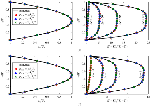
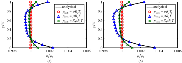
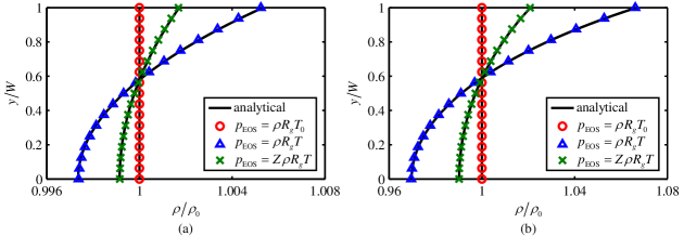
Fig. 2 shows the velocity and temperature distributions across the channel and compares the numerical results with the analytical solutions given by Eq. (32). Two sets of and are considered here: for the first set, is fixed at and varies from to ; while for the second set, is fixed at and varies from to . As an important computational parameter, the lattice Mach number, defined as , is fixed at in the simulations. Good agreement between the numerical results and the analytical solutions can be observed in Fig. 2, which demonstrates that the effects of the viscous dissipation and compression work are successfully captured by the present LB model. From Fig. 2, we can also see that the distributions of and obtained with different EOSs are almost identical, which agrees with the aforementioned discussion. Note that the simulation with and loses numerical stability for the ideal-gas EOS. To further validate the present LB model with self-tuning EOS, comparisons of the density distributions are carried out in Fig. 3. Good agreement is observed between the numerical results obtained with different EOSs and the corresponding analytical solutions given by Eq. (33), which demonstrates that various EOSs (including the nonideal-gas EOS) can be handled by the present LB model. For the decoupling EOS, keeps constant across the channel; as for the ideal-gas and Carnahan-Starling EOSs, varies across the channel due to the full coupling of thermo-hydrodynamic effects. In the Carnahan-Starling EOS, the molecular volume is considered, which implies that the rigid-sphere fluid is less compressible than the corresponding ideal gas. Therefore, the variation in density across the channel obtained with the Carnahan-Starling EOS is smaller than that obtained with the ideal-gas EOS, as clearly shown in Fig. 3.
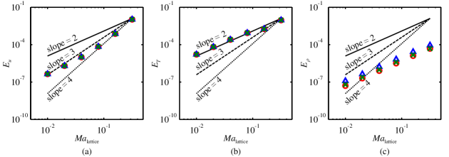
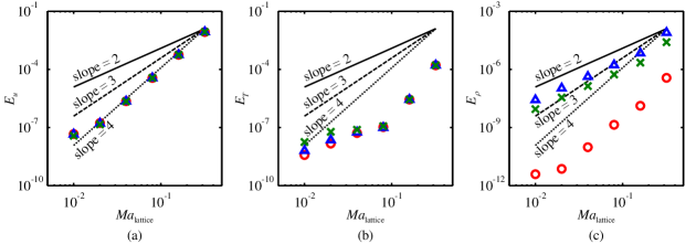
Considering that the lattice Mach number plays an important role in the LB method, we further investigate the accuracy of the present simulation with respect to . It is worth pointing out that the lattice Mach number is not only a computational parameter but also closely related to the Eckert number (or the real Mach number) due to the lattice sound speed given by Eq. (34). In the following simulations, the Prandtl number is fixed at , and the Eckert number is set as with varying from to . Thus, the temperature difference remains unchanged for different . The relative errors of velocity, temperature, and density are calculated here, which are defined as
| (36) |
where denotes the velocity , temperature , and density when , , and , respectively, the subscripts “numerical” and “analytical” denote the numerical result and analytical solution of , respectively, and the summation is over the computational domain. The relative errors , , and versus are shown in Fig. 4. As seen, the accuracy with respect to for velocity is fourth order when is relatively large and gradually decreases to second order as decreases, while the accuracy for temperature and density keep second order. Here, the fourth-order accuracy for when is relatively large is due to the elimination of the additional cubic terms of velocity, and the second-order accuracy may be caused by the boundary condition treatment. Nevertheless, from Fig. 4 we can clearly see that satisfying results with different EOSs can be obtained by the present LB model and boundary condition treatment under the low Mach number condition.
4.2 Thermal Couette flow
The thermophysical properties (dynamic viscosity and thermal conductivity) are assumed to be constant for the above thermal Poiseuille flow. To validate that the present LB model is capable of handling the coupled thermo-hydrodynamic flows with variable thermophysical properties, the thermal Couette flow between two parallel walls is simulated in this section. The lower wall is at rest and keeps adiabatic, and the upper wall moves along -direction with a constant velocity and keeps at a constant temperature . The Prandtl number and the specific heat at constant pressure are assumed to be constant, and thus . Considering a linear dependence of on that is , the analytical solutions for velocity and temperature are given as [47]
| (37a) | |||
| (37b) |
where is the channel width, and is an equivalent Mach number different from but closely related to the lattice and real Mach numbers. As it can be seen from Eq. (37), the analytical solutions for and are fully determined by and . Similarly to the thermal Poiseuille flow, the analytical solution for density here is not only related to the initial state, but it also depends on the adopted EOS. In the simulations, the density, velocity, temperature, and pressure are initialized as , , , and , respectively. Thus, the analytical solution for density is also given by Eq. (33), where the coefficient can be explicitly written as .
In the simulations, all the simulation parameters are chosen the same as those for the thermal Poiseuille flow, except that is fixed at for . Since varies with , also varies with even for the decoupling EOS. Fig. 5 gives the velocity and temperature distributions across the channel for and varying from to , and for and varying from to . Here, the simulation with and also loses numerical stability for the ideal-gas EOS. As seen in Fig. 5, the numerical results are in good agreement with the analytical solutions. Thus, the coupled thermo-hydrodynamic flows with variable thermophysical properties can be successfully handled by the present LB model. Fig. 5 also verifies that the results ( and ) obtained with different EOSs are indistinguishable as long as the simulations are numerically stable. Fig. 6 compares the distributions of density obtained with different EOSs for and , and for and . Good agreement between the numerical results and the corresponding analytical solutions can be observed, which reaffirms the applicability and accuracy of the present LB model with self-tuning EOS.
The accuracy of the present simulation with respect to the lattice Mach number is also investigated here. Considering the specific heat at constant pressure given by Eq. (35), we have . In the following simulations, the Prandtl number is fixed at , and the lattice Mach number varies from to . Fig. 7 shows the variations of the relative errors , , and with . Here, the relative error (, , and ) is also computed via Eq. (36), in which denotes , , and when , , and , respectively. It can be seen from Fig. 7(a) that the accuracy with respect to for velocity is fourth order and decreases to second order when and also are very small. A similar trend can also be observed in Fig. 7(b) for the accuracy for temperature . As to the accuracy for density , it is fourth order and decreases rapidly when is rather small for the decoupling EOS, while it is second order for the ideal-gas and Carnahan-Starling EOSs. Here, the observed high-order accuracy with respect to can be explained by the elimination of the additional cubic terms of velocity in the recovered momentum conservation equation, and the deterioration of accuracy when and also (, , and ) are very small is probably caused by the boundary condition treatment.
4.3 Natural convection in a square cavity
To further validate the present LB model for coupled thermo-hydrodynamic flows, the natural convection in a square cavity with a large temperature difference is simulated in this section. All the four walls of the cavity are at rest, among which the left (heating) and right (cooling) walls keep at the temperature and (), respectively, and the horizontal walls keep adiabatic. The temperature difference between the heating and cooling walls is quantified by a dimensionless parameter , where the reference temperature . The ideal-gas EOS is adopted here, and thus . The specific heat ratio and the Prandtl number are assumed to be constant. The dependence of dynamic viscosity on temperature is described by Sutherland’s law as follows [48]
| (38) |
where , , and is the dynamic viscosity at . As a key dimensionless parameter associated with natural convection, the Rayleigh number is defined as
| (39) |
where is the gravity acceleration, is the side length of the square cavity, and is the reference dynamic viscosity at . Initially, the ideal gas in the cavity stays still with temperature and density , and then the temperature of the left and right walls are abruptly changed to and , respectively. In the simulations, the lattice sound speed is set as , and the basic parameters are chosen as , , , and with . The Rayleigh number varies from up to , while the remaining dimensionless parameters are fixed at , , and . The grid sizes and the viscosity ratio adopted for different are listed in Table 1, where is set to and for and , respectively, to enhance the numerical stability and it is simply set to for . As to the velocity and temperature boundary conditions on all the four walls, they are realized by the present boundary condition treatment with first-order extrapolation.
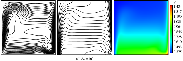
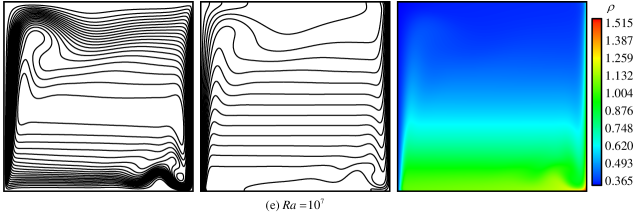
Fig. 8 shows the streamlines, isotherms, and density field for the natural convection when varies from to . It can be seen from Fig. 8 that a single vortex with its center closer to the cooling wall appears in the cavity for . As increases, the vortex is stretched by the natural convection and breaks up into two vortices when . As further increases, the two vortices move closer to the heating and cooling walls, respectively, and some small vortices are induced around the center and in the lower-right and upper-left corners of the cavity when . Meanwhile, a counter-rotating vortex also appears in the lower-right corner and very close to the lower wall for . When reaches , the natural convection becomes unsteady, and many small vortices, including some counter-rotating ones, are induced by the strong convection. As to the heat transfer characteristics, it can be seen from Fig. 8 that the isotherms are almost parallel to the vertical walls when , implying that the heat transfer is dominated by conduction. As increases, the isotherms around the cavity center progressively incline and become parallel to the horizontal walls, implying that the dominant mechanism for heat transfer changes from conduction to convection. When reaches , the isotherms spread along the heating and cooling walls in a very thin layer and become horizontal almost in the entire cavity. All these observed streamline patterns and isotherm characteristics are in good agreement with the previous numerical results [33, 35, 28, 29, 48], which are all obtained by the LB method except for the benchmark solutions reported in Ref. [48]. Note that the maximum reported in Refs. [33] and [35] are and , respectively, and the maximum reported in Refs. [28, 29, 48] are . On the basis of the present simulations, it is interesting to find that the natural convection in a square cavity with a large temperature difference () becomes unsteady when , while the corresponding natural convection with a small temperature difference (i.e., the Boussinesq approximation is valid) keeps steady when and becomes unsteady when [49, 50, 51]. From Fig. 8, we can also see that the density significantly varies over space, particularly in the vicinity of the cooling wall, with its minimum and maximum values smaller and larger than and , respectively. Obviously, the Boussinesq approximation cannot be adopted here. In addition, the density contours are similar to the isotherms to some extent, which conforms to the low Mach number condition [52]. In fact, the maximum Mach number is rather small for the natural convection simulated here [48].
![[Uncaptioned image]](/html/1809.08683/assets/x8.png)
![[Uncaptioned image]](/html/1809.08683/assets/x9.png)
![[Uncaptioned image]](/html/1809.08683/assets/x10.png)
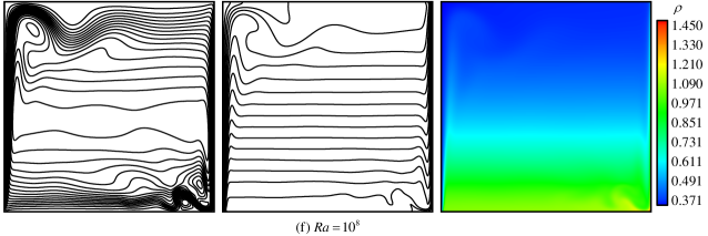
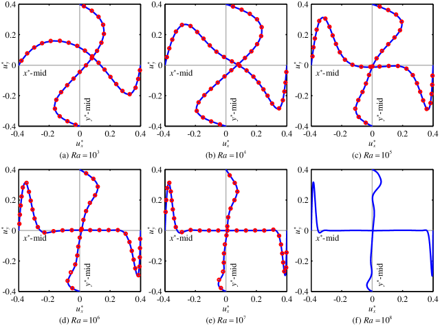
To further validate the present results, the profiles of the horizontal velocity along the vertical midplane and the vertical velocity along the horizontal midplane are plotted in Fig. 9 and compared with the benchmark solutions obtained by Vierendeels et al. [48] using the finite difference (FD) method. Here, the velocity and coordinate are normalized by the reference velocity and side length , respectively, i.e., and . Note that the convection becomes unsteady when , and thus Fig. 9(f) shows the instantaneous profiles at some time point. Excellent agreement between the present results and the benchmark solutions can be observed. From Fig. 9, we can also see that the velocity profiles are asymmetric with respect to the cavity center, which is caused by the invalidation of the Boussinesq approximation. For quantitative comparison, the average Nusselt number along the heating wall, the average pressure in the cavity, and the maximum horizontal (vertical) velocity and its position along the vertical (horizontal) midplane are computed and listed in Table 2. Here, the average Nusselt number and pressure are defined as
| (40a) | |||
| (40b) |
where is the local heat flux in , is the thermal conductivity at , and the pressure is normalized by . As seen in Table 2, the present results agree well with the previous numerical results, which further demonstrates the applicability and accuracy of the present LB model for coupled thermo-hydrodynamic flows.
| Method | |||||||
|---|---|---|---|---|---|---|---|
| Present | |||||||
| FD method [48] | |||||||
| LB method [35] | – | ||||||
| LB method [33] | – | ||||||
| Present | |||||||
| FD method [48] | |||||||
| LB method [35] | – | ||||||
| LB method [33] | – | ||||||
| Present | |||||||
| FD method [48] | |||||||
| LB method [35] | – | ||||||
| LB method [33] | – | ||||||
| Present | |||||||
| FD method [48] | |||||||
| LB method [35] | – | ||||||
| Present | |||||||
| FD method [48] | |||||||
| Present |
5 Conclusions
A novel LB model for coupled thermo-hydrodynamic flows is developed in the framework of the DDF approach. The velocity field is solved by the recently developed LB equation for density DF, by which the recovered EOS can be self-tuned via a built-in variable, implying that various EOSs can be adopted in real applications. With the energy conservation equation properly reformulated, a novel LB equation for total energy DF is directly developed at the discrete level to solve the temperature field. The viscous dissipation is recovered along with the conduction term by introducing a density-DF-related term into this LB equation, while the compression work is recovered along with the convection term by devising the equilibrium moment function for total energy DF. The work done by force is absorbed into the source term and then correctly incorporated into the LB equation via the discrete source term. Moreover, by modifying the collision matrix, the targeted energy conservation equation can be recovered without deviation term. The development of the present LB model, with double MRT collision schemes employed, is based on the standard lattice, and both the Prandtl number and specific heat ratio can be arbitrarily adjusted. On the basis of judiciously decomposing DF into its equilibrium, force (source), and nonequilibrium parts, boundary condition treatment is further proposed for simulating coupled thermo-hydrodynamic flows, which can ensure the local conservation of mass, momentum, and energy at the boundary node. The applicability and accuracy of the present LB model with self-tuning EOS are first validated by simulating thermal Poiseuille and Couette flows with the decoupling, ideal-gas, and Carnahan-Starling EOSs. Then, the present LB model is successfully applied to the simulation of natural convection in a square cavity with a large temperature difference for the Rayleigh number ranging from up to , and the obtained results agree very well with the previous benchmark solutions.
Acknowledgements
R.H. acknowledges the support by the Alexander von Humboldt Foundation, Germany. This work was also supported by the National Natural Science Foundation of China through Grant No. 51536005.
Appendix A Chapman-Enskog analysis
The detailed Chapman-Enskog analysis of the LB equation for density DF (i.e., Eq. (2)) can be found in our previous work [36]. Here, the Chapman-Enskog analysis of the LB equation for total energy DF (i.e., Eq. (18)) is carried out to recover the corresponding macroscopic conservation equation. For this purpose, performing the Taylor series expansion of centered at in Eq. (18a), and then transforming the result into moment space and combining it with Eq. (18b), we have
| (41) |
where . With the following Chapman-Enskog expansions [53]
| (42a) | |||
| (42b) |
we have , , and , where is the small expansion parameter. Substituting these expansions into Eq. (41), the , , and equations can then be obtained as
| (43a) | |||
| (43b) | |||
| (43c) |
where is introduced to simplify the descriptions.
From the equation (i.e., Eq. (43a)) and considering (see Eq. (17)), we have
| (44) |
which indicates that the () terms of the conserved moment satisfy
| (45) |
The equation for , extracted from Eq. (43b), is given as
| (46) |
which can be simplified as follows
| (47) |
Similarly, the equation for , extracted from Eq. (43c), is given as
| (48) |
where the repeated index implies summation from to . With Eq. (45), Eq. (48) can be simplified as follows
| (49) |
where is the energy flux expressed as
| (50) |
in which the first and second terms will account for the heat conduction and viscous dissipation, respectively.
To simplify the heat conduction term in Eq. (50), we add the equation for to the equation for and the equation for to the equation for , and then combine the results together and finally have
| (51) |
Considering and , Eq. (51) can be simplified as
| (52) |
where and are commutative, implying that the heat conduction is correctly driven by the temperature gradient. To recover the viscous dissipation term via Eq. (50), we can directly set
| (53) |
where the viscous stress tensor is given by Eq. (15). Consequently, the nonzero elements in can be completely and uniquely determined (see Eq. (24)). On the basis of Eqs. (52) and (53), can be written as
| (54) |
Combining the and equations (i.e., Eqs. (47) and (49)), as well as considering Eq. (54), the following macroscopic conservation equation can be recovered
| (55) |
Therefore, the heat conductivity is . Compared with the targeted energy conservation equation (i.e., Eq. (14)), no deviation term exists in Eq. (55) due to the modification of the collision matrix .
Appendix B Inverse matrix
The inverse matrix of is
| (56) |
where denotes the diagonal part of . The inverse matrix of is
| (57) |
where denotes the diagonal part of .
Appendix C Implementation
The detailed implementation of the collision process for density DF (i.e., Eq. (2b)) can be found in our previous work [36]. Here, a similar implementation of the collision process for total energy DF (i.e., Eq. (18b)) is given. In real applications, Eq. (18b) can be executed in the following sequence
-
1.
-
2.
-
3.
-
4.
where “” indicates assignment, and steps (2) and (4) correspond to the modification of collision matrix and the consideration of viscous dissipation, respectively. In step (4), (, , and ) can be directly obtained from the collision process for density DF. From the above discussion, it can be seen that the present collision process is easy to implement with high efficiency although the modified collision matrix is nondiagonal.
References
- [1] C. K. Aidun, J. R. Clausen, Lattice-Boltzmann method for complex flows, Annu. Rev. Fluid Mech. 42 (2010) 439–472.
- [2] M. Gross, R. Adhikari, M. E. Cates, F. Varnik, Thermal fluctuations in the lattice Boltzmann method for nonideal fluids, Phys. Rev. E 82 (2010) 056714.
- [3] R. Huang, H. Wu, Total enthalpy-based lattice Boltzmann method with adaptive mesh refinement for solid-liquid phase change, J. Comput. Phys. 315 (2016) 65–83.
- [4] I. Ginzburg, Equilibrium-type and link-type lattice Boltzmann models for generic advection and anisotropic-dispersion equation, Adv. Water Resour. 28 (2005) 1171–1195.
- [5] P. J. Dellar, D. Lapitski, S. Palpacelli, S. Succi, Isotropy of three-dimensional quantum lattice Boltzmann schemes, Phys. Rev. E 83 (2011) 046706.
- [6] Z. Chai, N. He, Z. Guo, B. Shi, Lattice Boltzmann model for high-order nonlinear partial differential equations, Phys. Rev. E 97 (2018) 013304.
- [7] G. R. McNamara, G. Zanetti, Use of the Boltzmann equation to simulate lattice-gas automata, Phys. Rev. Lett. 61 (1988) 2332–2335.
- [8] X. Shan, H. Chen, Lattice Boltzmann model for simulating flows with multiple phases and components, Phys. Rev. E 47 (1993) 1815–1819.
- [9] A. J. C. Ladd, Numerical simulations of particulate suspensions via a discretized Boltzmann equation. Part 1. Theoretical foundation, J. Fluid Mech. 271 (1994) 285–309.
- [10] X. He, L.-S. Luo, A priori derivation of the lattice Boltzmann equation, Phys. Rev. E 55 (1997) R6333–R6336.
- [11] X. He, L.-S. Luo, Theory of the lattice Boltzmann method: From the Boltzmann equation to the lattice Boltzmann equation, Phys. Rev. E 56 (1997) 6811–6817.
- [12] X. He, X. Shan, G. D. Doolen, Discrete Boltzmann equation model for nonideal gases, Phys. Rev. E 57 (1998) R13–R16.
- [13] L.-S. Luo, Unified theory of lattice Boltzmann models for nonideal gases, Phys. Rev. Lett. 81 (1998) 1618–1621.
- [14] X. He, S. Chen, G. D. Doolen, A novel thermal model for the lattice Boltzmann method in incompressible limit, J. Comput. Phys. 146 (1998) 282–300.
- [15] Z. Guo, C. Zheng, B. Shi, T. S. Zhao, Thermal lattice Boltzmann equation for low Mach number flows: Decoupling model, Phys. Rev. E 75 (2007) 036704.
- [16] X. Shan, Simulation of Rayleigh-Bénard convection using a lattice Boltzmann method, Phys. Rev. E 55 (1997) 2780–2788.
- [17] F. J. Alexander, S. Chen, J. D. Sterling, Lattice Boltzmann thermohydrodynamics, Phys. Rev. E 47 (1993) R2249–R2252.
- [18] G. R. McNamara, A. L. Garcia, B. J. Alder, A hydrodynamically correct thermal lattice Boltzmann model, J. Stat. Phys. 87 (1997) 1111–1121.
- [19] L. Zheng, B. Shi, Z. Guo, Multiple-relaxation-time model for the correct thermohydrodynamic equations, Phys. Rev. E 78 (2008) 026705.
- [20] P. Lallemand, L.-S. Luo, Theory of the lattice Boltzmann method: Acoustic and thermal properties in two and three dimensions, Phys. Rev. E 68 (2003) 036706.
- [21] A. Mezrhab, M. Bouzidi, P. Lallemand, Hybrid lattice-Boltzmann finite-difference simulation of convective flows, Comput. Fluids 33 (2004) 623–641.
- [22] A. Mezrhab, M. Amine Moussaoui, M. Jami, H. Naji, M. Bouzidi, Double MRT thermal lattice Boltzmann method for simulating convective flows, Phys. Lett. A 374 (2010) 3499–3507.
- [23] R. Huang, H. Wu, An immersed boundary-thermal lattice Boltzmann method for solid-liquid phase change, J. Comput. Phys. 277 (2014) 305–319.
- [24] D. Contrino, P. Lallemand, P. Asinari, L.-S. Luo, Lattice-Boltzmann simulations of the thermally driven 2D square cavity at high Rayleigh numbers, J. Comput. Phys. 275 (2014) 257–272.
- [25] M. Sbragaglia, R. Benzi, L. Biferale, H. Chen, X. Shan, S. Succi, Lattice Boltzmann method with self-consistent thermo-hydrodynamic equilibria, J. Fluid Mech. 628 (2009) 299–309.
- [26] S. Succi, Lattice Boltzmann 2038, Europhys. Lett. 109 (2015) 50001.
- [27] H. C. Lee, S. Bawazeer, A. A. Mohamad, Boundary conditions for lattice Boltzmann method with multispeed lattices, Comput. Fluids 162 (2018) 152–159.
- [28] Y.-L. Feng, S.-L. Guo, W.-Q. Tao, P. Sagaut, Regularized thermal lattice Boltzmann method for natural convection with large temperature differences, Int. J. Heat Mass Tran. 125 (2018) 1379–1391.
- [29] H. Safari, M. Krafczyk, M. Geier, A lattice Boltzmann model for thermal compressible flows at low Mach numbers beyond the Boussinesq approximation, Comput. Fluids, doi:10.1016/j.compfluid.2018.04.016.
- [30] X. Shan, X. F. Yuan, H. Chen, Kinetic theory representation of hydrodynamics: A way beyond the Navier-Stokes equation, J. Fluid Mech. 550 (2006) 413–441.
- [31] L.-H. Hung, J.-Y. Yang, A coupled lattice Boltzmann model for thermal flows, IMA J. Appl. Math. 76 (2011) 774–789.
- [32] N. I. Prasianakis, I. V. Karlin, Lattice Boltzmann method for thermal flow simulation on standard lattices, Phys. Rev. E 76 (2007) 016702.
- [33] Q. Li, K. H. Luo, Y. L. He, Y. J. Gao, W. Q. Tao, Coupling lattice Boltzmann model for simulation of thermal flows on standard lattices, Phys. Rev. E 85 (2012) 016710.
- [34] Y. Feng, P. Sagaut, W. Tao, A three dimensional lattice model for thermal compressible flow on standard lattices, J. Comput. Phys. 303 (2015) 514–529.
- [35] L. Fei, K. H. Luo, Cascaded lattice Boltzmann method for thermal flows on standard lattices, Int. J. Therm. Sci. 132 (2018) 368–377.
- [36] R. Huang, H. Wu, N. A. Adams, Lattice Boltzmann model with self-tuning equation of state for multiphase flows, arXiv:1809.02390 [physics.comp-ph].
- [37] Y. H. Qian, D. d’Humières, P. Lallemand, Lattice BGK models for Navier-Stokes equation, Europhys. Lett. 17 (1992) 479.
- [38] P. Lallemand, L.-S. Luo, Theory of the lattice Boltzmann method: Dispersion, dissipation, isotropy, Galilean invariance, and stability, Phys. Rev. E 61 (2000) 6546–6562.
- [39] R. Huang, H. Wu, N. A. Adams, Eliminating cubic terms in the pseudopotential lattice Boltzmann model for multiphase flow, Phys. Rev. E 97 (2018) 053308.
- [40] R. Huang, H. Wu, Phase interface effects in the total enthalpy-based lattice Boltzmann model for solid-liquid phase change, J. Comput. Phys. 294 (2015) 346–362.
- [41] R. Huang, H. Wu, A modified multiple-relaxation-time lattice Boltzmann model for convection-diffusion equation, J. Comput. Phys. 274 (2014) 50–63.
- [42] T. Krüger, H. Kusumaatmaja, A. Kuzmin, O. Shardt, G. Silva, E. M. Viggen, The lattice Boltzmann method: Principles and practice, Springer International Publishing, 2017.
- [43] Z. Guo, C. Zheng, B. Shi, Non-equilibrium extrapolation method for velocity and pressure boundary conditions in the lattice Boltzmann method, Chin. Phys. 11 (2002) 366.
- [44] Z. Guo, C. Zheng, B. Shi, An extrapolation method for boundary conditions in lattice Boltzmann method, Phys. Fluids 14 (2002) 2007–2010.
- [45] N. F. Carnahan, K. E. Starling, Equation of state for nonattracting rigid spheres, J. Chem. Phys. 51 (1969) 635–636.
- [46] R. Huang, H. Wu, Third-order analysis of pseudopotential lattice Boltzmann model for multiphase flow, J. Comput. Phys. 327 (2016) 121–139.
- [47] H. W. Liepmann, A. Roshko, Elements of gasdynamics, John Wiley & Sons, New York, 1957.
- [48] J. Vierendeels, B. Merci, E. Dick, Benchmark solutions for the natural convective heat transfer problem in a square cavity with large horizontal temperature differences, Int. J. Numer. Meth. Heat Fluid Flow 13 (2003) 1057–1078.
- [49] S. Paolucci, D. R. Chenoweth, Transition to chaos in a differentially heated vertical cavity, J. Fluid Mech. 201 (1989) 379–410.
- [50] D. A. Mayne, A. S. Usmani, M. Crapper, finite element solution of unsteady thermally driven cavity problem, Int. J. Numer. Meth. Heat Fluid Flow 11 (2001) 172–194.
- [51] R. Huang, H. Wu, Multiblock approach for the passive scalar thermal lattice Boltzmann method, Phys. Rev. E 89 (2014) 043303.
- [52] H. Paillere, C. Viozat, A. Kumbaro, I. Toumi, Comparison of low Mach number models for natural convection problems, Heat and Mass Transfer 36 (2000) 567–573.
- [53] S. Chapman, T. G. Cowling, The mathematical theory of non-uniform gases, 3rd Edition, Cambridge University Press, Cambridge, 1970.