How to tell an accreting boson star from a black hole

Abstract

The capability of the Event Horizon Telescope (EHT) to image the nearest supermassive black hole candidates at horizon-scale resolutions offers a novel means to study gravity in its strongest regimes and to test different models for these objects. Here, we study the observational appearance at 230 GHz of a surfaceless black hole mimicker, namely a non-rotating boson star, in a scenario consistent with the properties of the accretion flow onto Sgr A*. To this end, we perform general relativistic magnetohydrodynamic simulations followed by general relativistic radiative transfer calculations in the boson star space-time. Synthetic reconstructed images considering realistic astronomical observing conditions show that, despite qualitative similarities, the differences in the appearance of a black hole – either rotating or not – and a boson star of the type considered here are large enough to be detectable. These differences arise from dynamical effects directly related to the absence of an event horizon, in particular, the accumulation of matter in the form of a small torus or a spheroidal cloud in the interior of the boson star, and the absence of an evacuated high-magnetization funnel in the polar regions. The mechanism behind these effects is general enough to apply to other horizonless and surfaceless black hole mimickers, strengthening confidence in the ability of the EHT to identify such objects via radio observations.

1 Introduction

Observations of the Galactic Centre have confirmed the existence of a supermassive compact object at the radio source Sgr A*. Stellar motions have constrained its mass to $\approx 4\times 10^{6}\,{\rm M}_{\odot}$ (Ghez et al., 2008; Gillessen et al., 2009; Chatzopoulos et al., 2015; Boehle et al., 2016; Abuter et al., 2018a, 2020) and its density to $\approx 6\times 10^{15}\,{\rm M}_{\odot}\,\mathrm{pc}^{-3}$ (Ghez et al., 2008), favouring the hypothesis of a single massive object. Moreover, its low luminosity combined with its estimated accretion rate indicates the absence of an emitting hard surface (Marrone et al., 2007; Broderick et al., 2009). All of these features are consistent with a supermassive black hole (SMBH) as those believed to exist at the centres of most galaxies. Furthermore, flaring activity observed by the GRAVITY-Very Large Telescope Interferometer has been shown to be consistent with orbital motions near Sgr A*’s last stable circular orbit (Abuter et al., 2018b). International efforts from the Event Horizon Telescope Collaboration (EHTC; Doeleman et al., 2008; Akiyama et al., 2015; Fish et al., 2016) and BlackHoleCam (Goddi et al., 2017) successfully applied very-long-baseline interferometry (VLBI) techniques to obtain the first ever images of the SMBH candidate in the nearby galaxy M87 at a resolution comparable to the size of its event horizon (EHTC, 2019a, b, c, d, e, f), and data are currently being processed to obtain analogous images for Sgr A*. The M87 observations are consistent with the expectations for a Kerr black hole (EHTC, 2019a, e, f), namely, a “crescent” or ring-like feature, consisting of a dark region (associated with the “shadow” of the black hole) obscuring the lensed image of a bright accretion flow (Cunningham & Bardeen, 1973; Falcke et al., 2000; Grenzebach, 2016). The shape of this dark region can be exploited either to determine the properties of the black hole within the Kerr assumption (EHTC, 2019e, f), or to perform tests of general relativity (Abdujabbarov et al., 2015; Psaltis et al., 2015b; Younsi et al., 2016; Psaltis et al., 2016), a possibility assessed for Sgr A* by Mizuno et al. (2018) in a realistic scenario for the 2017 EHTC campaign and for near-future observations.

Even though the observations of the EHTC are consistent with the image expected from an accreting Kerr black hole, it is important to consider whether qualitatively similar images can be associated with other kinds of compact objects, and if so, how they could be distinguished from a Kerr black hole. Black holes are not the only objects predicted by general relativity that satisfy the constraints given by the aforementioned properties of Sgr A*, i.e., (1) being able to grow to millions of solar masses, (2) being extremely compact, and (3) lacking a hard surface. Some examples include: geons (Wheeler, 1955; Brill & Hartle, 1964; Anderson & Brill, 1997), oscillatons (Seidel & Suen, 1991; Ureña-López, 2002), Q-balls (Kleihaus et al., 2005) and compact configurations of self-interacting dark matter (Saxton et al., 2016). Allowing for the presence of a surface, the list of plausible compact objects can be expanded to include ultracompact objects with exotic surface properties, such as gravastars (Mazur & Mottola, 2004; Cattoen et al., 2005; Chirenti & Rezzolla, 2008, 2016). While for black holes the photon ring plays an important role in the formation of the shadow, it has been shown that horizonless objects that are compact enough to produce photon rings are unstable on short time-scales and under very general conditions, and are thus not viable as alternatives to SMBHs (Cunha et al., 2017b). Nevertheless, there is room for compact objects other than black holes to produce dark regions that effectively appear as shadows, as shown for example by Vincent et al. (2016) for the case of boson stars.

Boson stars are compact objects resulting from self-gravitating scalar fields, and are a very interesting case due to the ubiquity of scalar fields in cosmology (Albrecht & Steinhardt, 1982; Linde, 1982; Preskill et al., 1983; Matos & Guzman, 2000; Hui et al., 2017), string theory (Arvanitaki et al., 2010), and extensions of general relativity such as scalar-tensor theories (Fujii & ichi Maeda, 2003). Several authors have explored the possibility that supermassive boson stars could exist at the centres of galaxies or act as black hole mimickers (see e.g.,  Schunck & Liddle, 1997; Schunck & Mielke, 1999; Capozziello et al., 2000; Schunck & Torres, 2000; Torres et al., 2000; Guzmán, 2005; Vincent et al., 2016). Consequently, a number of studies have investigated the signatures of such objects, which include the dynamics of accreted particles (Schunck & Torres, 2000), the gravitational redshift (Schunck & Liddle, 1997), and lensing (Virbhadra et al., 1998; Dabrowski & Schunck, 2000; Virbhadra & Ellis, 2000; Cunha et al., 2015; Cunha et al., 2017a) of radiation emitted within the boson star, and the stellar orbits around them (Grould et al., 2017). Guzmán (2006, 2011) studied spectra of alpha-discs (Shakura & Sunyaev, 1973) around boson stars, reporting the absence of a clear signature distinguishing them from black holes. Motivated by the then forthcoming observations of the EHTC, Vincent et al. (2016) reached similar conclusions by comparing strong-field images of stationary tori in equilibrium around a Kerr black hole and several boson stars. Specifically, they found that a central dark region that mimics the shape and size of a black hole shadow may appear for boson stars as a result of lensing of the empty space around which the torus orbits. On the basis of this set-up, it was concluded that boson stars would be very difficult to distinguish from black holes by means of strong field images. While these considerations are correct given the physical scenario considered, it is clear that the latter does not account for the dynamics of the matter that from the torus will accrete towards the centre of the boson star. Indeed, uncountable astronomical observations – and numerous numerical simulations – clearly indicate that quasi-stationary accretion process accompany the dynamics of tori around compact objects. Furthermore, the existence of stable circular orbits at all radii, at least for spherically symmetric boson stars (Guzmán, 2006), makes the choice of the inner radius of the equilibrium torus arbitrary, whereas in a realistic situation the accreted plasma is able to reach all regions within the boson star interior.

Numerical simulations of unmagnetized zero angular momentum accretion flows onto boson stars were carried out by Meliani et al. (2016), finding a significantly different behaviour with respect to black holes as a result of the absence of an event horizon. Specifically, they observed a polar outflow produced by the collision of matter infalling radially from the disc. However, this study did not include a systematic investigation of the discernibility of the emission from the two compact objects via ray-traced images. Moreover, accretion onto astrophysical compact objects is believed to occur as a result of a gradual loss of angular momentum from orbiting matter driven by the magnetorotational instability (MRI; Balbus & Hawley, 1991), and radiation at the observing frequencies of VLBI experiments is mainly produced by synchrotron emission. Therefore, the inclusion of magnetic fields is essential to realistically simulate VLBI observations.

We revisit the question of the observational appearance at 230 GHz of a boson star at the Galactic Centre, and of its distinguishability from an SMBH. To this end, we produce strong-field synthetic EHTC images of accreting black holes and of an accreting boson star, modelling the accretion flow by means of fully dynamic general relativistic ideal magnetohydrodynamic (GRMHD) simulations. Together with considering the plasma configurations that arise from the same turbulent processes believed to occur in nature, these simulations allow us to understand the dynamics of accretion flows onto horizonless and surfaceless compact objects, and to identify those features that could appear in situations that are more general than the particular boson star case considered here.

Using the results of these simulations, we also perform general relativistic radiative transfer calculations and produce synthetic images accounting for realistic EHTC observations. As we will highlight in what follows, we conclude that under these conditions, it is possible to discriminate between an accreting black hole and the boson star considered in this study by means of VLBI observations. In particular, we show that this distinction is possible because accretion onto the boson stars considered here leads to the accumulation of matter down the innermost regions of the compact object. Indeed, because matter can even reach the centre of the boson star, emission will be present at all radii and dark regions in the image – if they exist at all – are much smaller than those coming from black holes having the same mass. On the basis of these considerations it is possible to state quite generically that although horizonless and surfaceless objects can form dark regions that are qualitatively similar to the shadow of a black hole, these will be smaller than that expected size of the shadow of a black hole of the same mass under very general circumstances.

2 Initial data and numerical set-up

We simulate numerically in three spatial dimensions (3D) the accretion from a magnetized torus onto a Kerr black hole with total angular momentum $J$, a Schwarzschild black hole, and two cases of non-rotating boson stars, all with the same mass $M$. The Kerr black hole has a dimensionless spin parameter $a:=J/M^{2}=0.9375$ (we use units with $G=c=1$). Although results relative to the Schwarzschild black hole case will also be presented, we first focus our discussion on the comparison between the non-rotating boson star and the Kerr black hole.

There are two reasons behind this choice. First, rotating boson stars are computationally more difficult to generate, requiring the solution of a system of elliptic partial differential equations instead of the ordinary differential equations that describe non-rotating models. Being this is the first self-consistent study of the observational properties of accreting boson stars, we decided to start with the simplest configuration – a non-rotating boson star with a simple quadratic potential, i.e., a “mini boson star” – and to leave others for future work. As will be explained below, this has lead us to results that are applicable to some extent to more general situations. In addition, this approximation might not be so severe in light of the fact that very compact horizonless objects, including boson stars, cannot be rapid rotators since they are subject to a dynamical instability when rotating fast enough to produce ergoregions (Comins & Schutz, 1978; Yoshida & Eriguchi, 1996; Cardoso et al., 2008; Chirenti & Rezzolla, 2008). The more compact the boson star, the smaller the spin parameter required to produce an ergoregion and hence an instability. Furthermore, recent numerical studies suggest that even slowly rotating configurations collapse either to Kerr black holes or to non-rotating boson stars, due to a fast instability possibly related to their topology (Sanchis-Gual et al., 2019). The existence of this instability in the non-linear regime is supported by the fact that rapidly rotating boson stars are not found as endpoints in the evolution of merging binaries (Bezares et al., 2017; Palenzuela et al., 2017). Second, for non-rotating mini boson stars, the absence of a surface or a capture cross section permits stable circular orbits for massive particles down to the centre of the boson star. From an observational point of view, this is expected to lead to smaller source sizes, with emission concentrated near the center. On the other hand, the size of a black hole image is closely related to that of its shadow, which, in turn, is smaller for rapidly spinning black holes. Hence, the image of a rapidly rotating black hole will be closer in size to that of a non-rotating boson star having the same mass, making the issue of the distinguishability much more relevant. In addition, it is possible that the complex lensing patterns that can be generated by rotating boson stars (Cunha et al., 2015; Cunha et al., 2017a; Vincent et al., 2016) would produce images that are more easily distinguishable from those of black holes. Overall, these considerations all suggest that interpreting strong field images is most challenging when comparing a non-rotating boson star and a rapidly rotating black hole.

As mentioned above, the two boson star space-times considered here are solutions of the Einstein–Klein–Gordon system in spherical symmetry for the potential of a mini boson star (Kaup, 1968) (more information on the methods used to obtain these solutions is given in Appendix A). For the first of these two models, which hereafter we will refer to as “model A”, the 99 per cent compactness is $\mathcal{C}_{99}\coloneqq M_{99}/R_{99}=0.098$, where $R_{99}$ is the radius within which $99\%$ of the mass ($M_{99}$) is contained. On the other hand, the second model, which we will refer to as “model B”, has a compactness $\mathcal{C}_{99}=0.075$. While these compactnesses are not the largest that can be achieved for boson stars, they are among the most compact boson stars with a quadratic potential, for which the maximum limit is $\approx 0.11$, or $\approx 0.08$ for stable configurations.

It is worth mentioning that although $\mathcal{C}_{99}$ is widely used to have a rough idea of how compact and hence “relativistic” a compact object is, for objects with large variations in density such as boson stars, its value could vary considerably if a different percentage of the mass is considered. Overall, and as it will be shown in section 3 and in Appendix B, the two boson star models considered here are useful and representative cases of the two distinct behaviours of the accretion flow that are possible for a surfaceless compact object.

To simulate the accretion flow we use the publicly available code bhac (Porth et al., 2017; Olivares et al., 2019, www.bhac.science), which solves the equations of GRMHD in arbitrary stationary space-times using state-of-the-art numerical methods. The plasma follows an ideal-fluid equation of state with adiabatic index $\hat{\gamma}=4/3$ (Rezzolla & Zanotti, 2013). Random perturbations are added to the initial equilibrium torus to trigger the MRI and allow accretion. Details on the construction of the tori, and the choices made in order to perform a fair comparison and to ensure a proper resolution of the MRI are provided in Appendix C. Finally, since the mass of the accretion disc is negligible when compared to that of the compact object (test fluid approximation), the space-time can be considered fixed and the scalar field has no interaction with the fluid or the electromagnetic field besides the gravitational one.

3 Numerical results

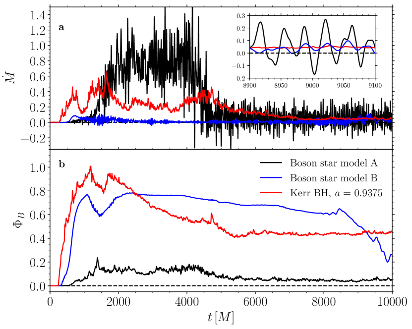
Figure 1: Evolution of the mass accretion rate (a) and the absolute magnetic flux (b) through the outer event horizon for the Kerr black hole and through a spherical shell at $r=2\,M$ for the two boson stars, in dimensionless units. The inset in panel (a) reports the mass accretion rate in the time window between $t=8900\ M$ and $9100\ M$. Note that mass accretion rate becomes quasi-stationary after $t\simeq 6000\,M$ and that the accretion rate can also be negative for the boson stars. The drop in magnetic flux between $t/M\in[8000,10000]$ for boson star model B is due to a rearrangement of the internal magnetic field of the boson star and is discussed in more detail in Appendix B.3.

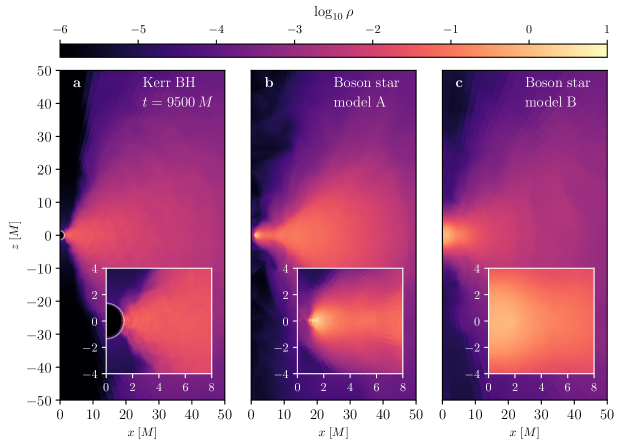
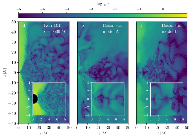
Figure 2: Rest-mass density in the fluid frame (panels a, b and c) and logarithmic plasma magnetization $\sigma=b^{2}/\rho$ (panels d, e and f) at $t=9500\,M$, for the Kerr black hole (a and d), and boson star models A (b and e) and B (c and f). The black hole horizon is marked by a white line and its excised interior is shown in solid black.

As mentioned in section 2, from now on we will focus on the comparison between the Kerr black hole case and that of the two non-rotating boson stars. Fig. 1 reports in arbitrary units the evolution of the mass accretion rate $\dot{M}$ (panel a) and of the absolute magnetic flux ${\Phi}_{{}_{B}}$ threading a surface at $r=r_{0}$ (panel b):

$$\dot{M} :=-\int_{r_{0}}\rho u^{r}\sqrt{-g}\,d\theta d\phi\,,$$ (1)

$${\Phi}_{{}_{B}} :=\frac{1}{2}\int_{r_{0}}|B^{r}|\sqrt{-g}\,d\theta d\phi\,,$$ (2)

where $g$ is the metric determinant, $\rho$ is the rest-mass density of the fluid, $u^{r}$ is the radial component of its four-velocity, and $B^{r}$ is the radial component of the magnetic field in the Eulerian frame. In the case of the black hole, we take $r_{0}$ to be the radial coordinate of the outer horizon, while $r_{0}=2M$ for the boson stars. After the initial growth and saturation of the MRI at $t\simeq 1000\ M$, the mass accretion rate for each of the objects becomes quasi-stationary for $t\gtrsim 6000\ M$, oscillating around a small positive value. After $t=8000\ M$, a series of changes in the magnetic field structure of boson star model B reduce significantly the amount of magnetic flux crossing the detector shell. Although the state of the magnetic field cannot be described as quasi-stationary, total intensity images calculated before, during and after this event can be still considered representative, as it is discussed in Appendix B.3. Comparing the behaviour of mass accretion rate for the different objects it is possible to appreciate that while the black hole always has a positive $\dot{M}$, a boson star can also attain negative values. This is permitted at all radii due to the absence of an event horizon.

As we will discuss below, this outflow is due to oscillations of an internal configuration of matter accumulating within the boson star, whose geometric distribution can take either the shape of a mini torus (as in the case of model A) or of a mini cloud (for model B), depending on the properties of the space-time (see Appendix B for details). A magnified view of $\dot{M}$ during the quasi-stationary stage of the accretion is shown in the inset of Fig. 1 (a), highlighting these quasi-periodic inflows and outflows. For the case in which the stalled accretion is in the form of a mini torus (model A), we have found the typical frequency associated with the quasi-periodic oscillations in $\dot{M}$ to be very close to the epicyclic frequency at the inner edge of the mini torus. This is unsurprising since matter accumulates in this region and small perturbations there will trigger trapped p-mode oscillations that induce large excursions, both positive and negative, in the accretion rate (Rezzolla et al., 2003b, a). On the other hand, in the case in which the stalled accreting matter is in the form of a mini (spheroidal) cloud (model B), the oscillations in the accretion rate originate from the response of the central cloud when compressed by the accreting matter.

Figure 2 shows a snapshot at $t=9500\,M$ and on the meridional plane, of rest-mass density $\rho$ (panels a, b and c) and plasma magnetization $\sigma:=b^{2}/\rho$ (panels d, e and f), where $b$ is the magnitude of the magnetic field in the fluid frame. In each panel we contrast the behaviour of these quantities in the case of the Kerr black hole (panels a and d) with that of boson stars A (panels b and e) and B (panels c and f). As anticipated, a peculiar feature of the accretion onto the boson star of model A is the formation of a smaller torus, which is most clearly visible in the inset of panel (b) of Fig. 2. This small torus, which essentially represents a stalled portion of the accretion flow, is produced by the presence of both a steep centrifugal barrier and by the suppression of the MRI. In fact, we observe that for small radii, the orbital angular velocity decreases towards the centre, violating the criterion for the occurrence of the MRI and stalling matter at the radius where the angular velocity profile reaches a maximum (Balbus & Hawley, 1991). In Appendix B, we show that the formation of this structure can be related to the angular velocity profile of circular geodesics in the boson star space-time, which enables one to predict its size for other horizonless objects beyond mini boson stars.

On the other hand, in the case of the accretion onto the boson star of model B, this inversion in the rotation velocity profile does not occur, and MRI continues to drive accretion at all radii up to the origin, resulting in the accumulation of fluid at the centre, as can be seen in the inset of panel (c) in the same figure. An interesting question is how long it would take for these boson stars to accrete enough matter to form an SMBH. Although it is not possible to give an answer solely from a GRMHD simulation under the test fluid approximation, a very rough estimate will be given in Appendix B using the physical mass accretion rate, calculated in section 4.

As will be shown in section 4, in both of the boson star cases the accumulation of matter inside the would-be horizon, i.e., the region of space-time with $r<2M$, produces an emitting region with an intrinsic source size smaller than that expected for a black hole. Such smaller source-sizes can be expected to be produced under very general circumstances and would therefore provide a signature for distinguishing surfaceless black hole mimickers. As shown in Appendix B, this is the case for a large portion of the parameter space of mini boson stars, which includes the most compact and most relativistic stable configurations. In fact, although the images of model-A boson stars could be qualitatively similar to those of black holes, i.e., by showing ring-like structures in some situations, the dark region will be smaller than the shadow of a black hole with the same mass. However, for model-B boson stars, the effective absence of such dark regions would make their images even more strikingly different from those of black holes. In general therefore horizon and surfaceless compact objects are characterised by accretion flows reaching very small radii, so that the resulting electromagnetic emission will lead to very small source sizes and thus very compact dark regions.

It can also be noticed that though still orders of magnitude less dense than the rest of the simulation, the polar region in the boson star is much less clean than that of the black hole (Figs. 2a, b, and c). In fact, while the black hole’s gravity is able to evacuate the polar regions and capture matter, the hot plasma that has reached the inner regions of the boson star can become gravitationally unbound due to its thermal energy and flow out through the polar regions as a slowly moving wind with Lorentz factors $\Gamma\lesssim 1.05$. This outflow, however, is of a fundamentally different nature to that observed by Meliani et al. (2016), which – in a scenario with no magnetic fields or angular momentum – was instead caused by the pressure increase at the stellar centre due to matter accreted radially from the equatorial regions.

Another obvious property of the accretion flow onto our non-rotating boson stars is the very low magnetization present along the polar regions and that is more than two orders of magnitude smaller than in the corresponding black hole simulations. As a result, no significant jet is produced in both of our accreting boson star models. While this may be the result, in part, of the choice of non-rotating models, the mass-loss we measure is mostly due to the combination of the steep centrifugal barrier and of the large internal energy and the magnetic energies, rather than by a genuine MHD acceleration process, such as the one behind the Blandford–Znajek mechanism in rotating black holes (Blandford & Znajek, 1977).

On the other hand, the lack of clear signatures for the presence of a powerful relativistic jet in Sgr A* does still allow us to consider non-rotating boson stars as viable models to describe the compact object at the centre of our Galaxy. New GRMHD simulations are evidently needed in order to determine whether relativistic jets can be produced by rotating boson star models. We plan to investigate these scenarios in future works.

4 Ray-traced and synthetic images

We next discuss how to use the results of the GRMHD simulations to produce ray-traced and synthetic images at the EHTC observing frequency of $230\,{\rm GHz}$, assuming a population of relativistic thermal electrons at temperature $T_{\rm e}$, which emit synchrotron radiation and are also self-absorbed. Several parameters need to be fixed when converting the dimensionless quantities evolved numerically to produce physical images. We fix the compact object mass as $M=4.02\times 10^{6}\,{\rm M}_{\odot}\simeq 0.04\,{\rm AU}$ and the distance from the source as $7.86\,{\rm kpc}$ (Boehle et al., 2016). This sets the length and time scalings of the general relativistic radiative transfer calculations (see e.g.,  Younsi et al., 2012; Mizuno et al., 2018) and yields the appropriate flux scaling. Finally, we set the ion-to-electron temperature ratio $T_{\rm i}/T_{\rm e}=3$ (Mościbrodzka et al., 2009), and choose the compact object mass accretion rate $\dot{M}$ such that, at a resolution of $1024\times 1024$ pixels, the total integrated flux of the image reproduces Sgr A*’s observed flux of $\simeq 3.4\,{\rm Jy}$ at $230\,{\rm GHz}$ (Marrone et al., 2006). The mass accretion rates obtained after rescaling for each of the compact objects are displayed in Table 1. These values were computed as averages over the time interval $t/M\in[8900,\,10000]$, which, for Sgr A*, corresponds to an observing time of $\sim 6\,{\rm h}$. At these times and over these timescales, the GRMHD simulations have reached a state that can be considered representative (cf. Fig. 1 and discussion at the beginning of Section 3).

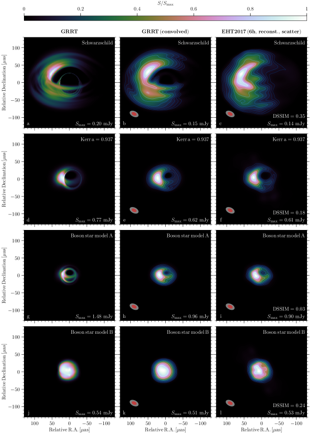
Figure 3: From top to bottom: ray-traced and synthetic images at $230\,{\rm GHz}$ and inclination angle of $\theta_{\rm obs}=60^{\circ}$ of the Schwarzschild black hole (first row), the Kerr black hole (second row), and boson star models A (third row) and B (fourth row). From left to right, first column: ray-traced images averaged over the interval $t/M\in[8900,\,10\ 000]$, second column: ray-traced images convolved with 50 per cent (red shaded ellipse) of the EHTC beam (grey shaded ellipse), third column: reconstructed images including interstellar scattering, convolved with $50\%$ (red shaded ellipse) of the EHTC beam (grey shaded ellipse) and indicating the value of the DSSIM metric.

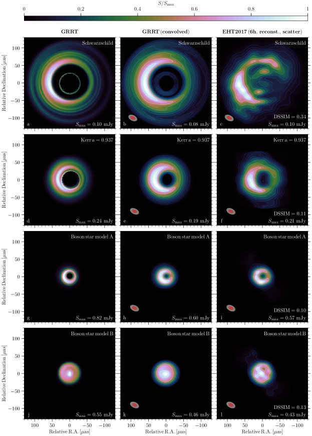
Figure 4: Same as Fig. 3 for an inclination angle of $\theta_{\rm obs}=15^{\circ}$.

Table 1: Physical mass accretion rates (in units of $10^{-10}{M}_{\odot}\,{\rm yr}^{-1}$), obtained after rescaling the dimensionless accretion rates of Fig. 1 to give an $\simeq 3.4\,{\rm Jy}$ flux at $230\,{\rm GHz}$ for the Kerr black hole and the two boson star models.

Object	$\theta_{\rm obs}={15}^{\circ}$	$\theta_{\rm obs}={60}^{\circ}$
Kerr BH	$34.40$	$8.19$
BS model A	$8.07$	$6.40$
BS model B	$1.40$	$1.46$

In this way, using the radiative transfer code bhoss (Younsi et al., 2020), and using the same time interval mentioned above, we produce images at several observing angles, but present here those at $\theta_{\rm obs}=60^{\circ}$ (Fig. 3), consistent with the observational constraints found by (Psaltis et al., 2015a), and $\theta_{\rm obs}=15^{\circ}$ (Fig. 4), which is within the constraint $\theta_{\rm obs}\leq 27^{\circ}$ given by hotspots models of GRAVITY observations (Abuter et al., 2018b).

We follow the same procedure to produce images for both a Kerr and a Schwarzschild black hole. The latter is used to highlight the fact that they differ more from those of the boson star, despite the closer similarities of the space-time. We note, however, that the larger image size caused by the more extended emitting region near the ISCO makes the images produced by a Schwarzschild black hole incompatible with present constraints on the source size of Sgr A*, i.e., $120\pm 34\ \mu{\rm as}$ (Issaoun et al., 2019).

More specifically, the various rows of Fig. 3 show the ray-traced and synthetic images at $230\,{\rm GHz}$ and inclination angle of $\theta_{\rm obs}=60^{\circ}$ of the Schwarzschild black hole (first row), the Kerr black hole (second row), and boson stars models A (third row) and B (fourth row). The different images can also be compared across columns. From left to right, in fact, we show the average of the ray-traced images in the interval $t/M\in[8900,\,10\ 000]$ (first column), the same ray-traced images convolved with 50% (red shaded ellipse) of the EHTC beam (grey shaded ellipse; second column), the reconstructed images including interstellar scattering, convolved with $50\%$ (red shaded ellipse) of the EHTC beam (grey shaded ellipse; third column) and indicating the value of the DSSIM metric. In a very similar fashion, Fig. 4 shows the equivalent images when an inclination angle of $\theta_{\rm obs}=15^{\circ}$ is considered.

The synthetic radio images have been generated using the ehtim software package (Chael et al., 2016) and after selecting as an observing array the configuration of the EHTC 2017 observing campaign (EHTC, 2019b), consisting of eight radio telescopes in North America, Europe, South America and the South Pole. To mimic realistic radio images, we follow closely the 2017 observing schedule, using an integration time of $12\,{\rm s}$, an on-source scan length of $7-10\,{\rm min}$ calibration, and pointing gaps between the on-source scans and a bandwidth of $4\,{\rm GHz}$. Within these constraints, we perform the synthetic observations of the Galactic Center on 2017 April 8th from 08:30 to 14:30 UT. The visibilities are computed by Fourier-transforming the general relativistic radiative transfer images and sampling them with the projected baselines of the array (Chael et al., 2016). During this calculation, we include thermal noise and $10\%$ gain variations, as well as interstellar scattering by a refracting screen (Johnson & Gwinn, 2015), as expected for the physical condition around Sgr A*. We reconstruct the final images using a maximum entropy method (MEM), provided with ehtim. In addition to the calculation of the synthetic images, we convolve the general relativistic radiative transfer images with 50% of the EHTC beam (second column in Fig. 3). These images can be used to examine the influence of the sparse sampling of the Fourier space and interstellar scattering on the reconstructed images (third column in Fig. 3).

Overall, the visual inspection of the reconstructed images (third columns in Figs. 3 and 4) shows clear differences between the four compact objects that can be summarised as follows. First, the black hole images – either from a Schwarzschild or a Kerr black hole – exhibit a “crescent” structure, i.e., a very asymmetric ring structure that is not present in the case of the boson stars, whose emission tends to be either of a quasi-uniform ring or of a uniform circle.

Second, the boson stars exhibit a smaller source size as a result of the emission from the small torus in its interior and thus at radii comparable or smaller than the black hole horizon. As mentioned in section 3, the location of the mini torus in the case of model-A boson stars is determined by the radius at which the angular velocity profile reaches a maximum. Therefore, and also for more compact boson stars for which the exterior space-time is increasingly similar to that of a black hole, the mini torus will be located at radii smaller than that of the event horizon, consistently yielding a smaller source size and a correspondingly smaller dark region as distinguishing image features.

Third, it is possible to use the phenomenology observed in the simulations involving boson star models A and B to calculate, in a general way, the size of the central dark region of the class of mini boson stars considered in this study (cf. Eq. 11). In this way, we find that for all the models considered it is significantly smaller than for black holes. Indeed, for some modes, such as the boson star model B, the dark region is even absent (see Appendix B for details).

Fourth, the boson stars generally yield a more symmetric image due to the absence of frame dragging, which significantly reduces Doppler boosting and consequently the sharp contrast in emission between material approaching and receding from the observer. Given that boson stars which are both compact and rapidly spinning are believed to be unstable, a higher symmetry is likely to be a common property of boson star images.

Finally, although less likely to be noticed by near-future observations and likely requiring space-based missions (see e.g.,  Roelofs et al., 2019), the boson star images lack a sharp transition between the middle dark region and its bright surroundings, which is a fundamental property of a black hole shadow and the narrow photon ring. In fact, due to the absence of a photon-capture cross-section, the central dark region in the case of boson star model A is simply a lensed image of the central low-density region.

A more quantitative assessment of the degree of similarity among the various images considered can be made by computing image-comparison metrics, such as the structural dissimilarity index (DSSIM; Wang et al., 2004). The DSSIM is computed between the convolved general relativistic radiative transfer images and the reconstructed ones and, to guarantee that we compare similar structures within both images, we perform an image alignment prior to its calculation and restrict to a field of view of 110 $\mu{\rm as}$. For an inclination of $60^{\circ}$, comparing the convolved Kerr image with the reconstructed image leads to a DSSIM of $0.18$ and in the case of the boson star model A we obtain a DSSIM of 0.03. The inter-model comparison, i.e., Kerr–model A and model A–Kerr, reveals DSSIMs of 0.31 and 0.63, respectively. Unsurprisingly, comparisons with the Schwarzschild black hole and with boson star model B produce significantly higher DSSIM values, as reported in Tables 2 and 3. Given these values, we conclude that the models could be distinguishable with current EHTC observations of Sgr A*.

Although we plan to address this issue in more detail in a future work, it may be interesting to briefly discuss what are the consequences of our study regarding the EHT 2017 observations of M87. The absence of a powerful jet immediately rules out the static boson star models considered here as feasible models for this source. However, focusing only on the strong-field imaging, we may contrast the EHT observations with the properties of boson star images predicted by our simulations. Boson stars of model B, namely those for which the images do not display a central dark region, and which comprises all of those in the stable branch, are in clear contrast with the EHT observations, which instead show a ring-like feature. On the other hand, boson stars of model A produce images with ring-like structures, but the size of the dark region would correspond to a much larger mass of the central object than for the case of black holes. According to the estimations given in Fig. 7 (see Appendix B.1), assuming the object is a boson star would yield a mass estimate that is $70-150\,\%$ larger than for a Kerr black hole, causing tension with the value obtained from stellar dynamics, which is in agreement with the Kerr hypothesis (EHTC, 2019a, e).

As a concluding remark we note that an additional tool to discriminate between the two objects comes from the variability of the emission (see Appendix B for details). Given the qualitative differences in the accretion rate, we also expect different properties in the energy spectra, as well as different closure-phase variabilities for the two objects. These differences will be particularly prominent in large antenna triangles, which probe the innermost regions currently accessible by the EHTC.

Table 2: DSSIM metric for the comparison between the convolved and reconstructed images at an observer inclination angle of $60^{\circ}$. Self-comparisons produce significantly smaller values than cross-comparisons, showing that images are distinguishable.

Convolved image	BH	BH	BS	BS
	($\emph{a}={0}$)	($\emph{a}={0.9375}$)	model A	model B
BH ($a=0$)	0.34	1.03	0.73	1.04
BH ($a=0.9375$)	0.97	0.18	0.31	0.50
BS model A	1.21	0.61	0.03	0.25
BS model B	1.96	0.87	0.13	0.24

Table 3: Same as Table 2. for an inclination angle of $15^{\circ}$.

Convolved image	BH	BH	BS	BS
	($\emph{a}={0}$)	($\emph{a}={0.9375}$)	model A	model B
BH ($a=0$)	0.34	0.82	1.22	1.01
BH ($a=0.9375$)	0.87	0.10	0.34	0.12
BS model A	1.16	0.26	0.10	0.28
BS model B	1.12	0.38	0.14	0.13

5 Conclusions

We have carried out the first 3D GRMHD simulations of disc accretion onto boson stars and combined them with general relativistic radiative transfer calculations, with the goal of determining whether, under realistic observing conditions such as those of the EHTC, an accreting non-rotating boson star can be distinguished from a black hole of the same mass. For the latter, we have considered both non-rotating and rotating black holes, focusing on the second ones as they provide more images that are more compact and hence closer to those produced by boson stars.

By comparing the images produced for the two compact objects using very similar set-ups, we found important differences, both in the plasma dynamics and in the general relativistic radiative transfer images. Indeed, the absence of a capturing surface in the case of boson stars, introduces important and fundamental differences in the flow dynamics. More specifically, matter accreting onto the boson stars can reach their innermost regions, attaining quasi-stationary configurations with either distributions that are either toroidal (i.e., a mini torus) or quasi-spheroidal (i.e., a mini cloud). This behaviour, which has not been reported before, is simply the result of the existence of stable orbits at all radii and to the suppression of the accretion process due to the suppression of the MRI and to the presence of a steep centrifugal barrier. In turn, this matter behaviour leads to the absence of an evacuated high-magnetization funnel in the polar regions and to images that show a markedly smaller source size and a more symmetric emission structure, in stark contrast to the characteristic crescent of the images resulting from the accretion onto black holes. As a result of these differences in the plasma dynamics and emission, we conclude that it is possible to distinguish the images of the accreting mini boson star models considered here from the corresponding images of accreting black holes having the same mass.

The results presented have been obtained for two representative cases of mini boson stars that are non-rotating and do not have a photon orbit. While other boson star models could be investigated – for instance, by considering more complex potentials leading to more compact solutions and even to the appearance of an unstable photon orbit – we believe that the results found here will continue to apply and be a generic property also as for other surfaceless and horizonless compact objects. This rationale is based on three important properties shared by these objects. First, horizonless and surfaceless objects permit the accumulation of matter within their interior. For monotonically decreasing angular velocity profiles, this accumulation will occur at the centre, while for angular velocity profiles having a maximum, this will occur at this maximum in the form of a stalled mini torus. As discussed in Appendix B.1, for very compact objects that have exterior space-times similar to those of black holes, this feature will generally occur at radii smaller than that of the event horizon of the corresponding black hole space-time, inevitably resulting in a smaller observed image size. Second, because horizonless compact objects rotating sufficiently fast to produce ergospheres are unstable, the asymmetry produced by Doppler boosting and related to the frame dragging in black hole images is likely to be less pronounced for horizonless objects. Finally, the central dark region that can be produced by these objects does not result from a photon capture cross-section as is the case for a black hole. Rather, it represents the lensed image of the central low-density region, which has a diffused boundary. As a result, the corresponding shadow can be expected to have a much reduced brightness contrast and a sharper edge, which can be properly revealed by imaging at increased resolutions. All of these considerations need to be corroborated by additional simulations, which we plan to perform in the near future. In particular, it would be very interesting to verify whether the complex lensing patterns produced by rotating boson stars – as those found by Vincent et al. (2016) and Cunha et al. (2017a) – do indeed facilitate distinguishing them from black holes, when produced in a realistic observational scenario.

Finally, we note that ongoing pulsar searches around Sgr A* (Kramer et al., 2004), when successful, could provide additional important information to the experiment outlined here. A suitable pulsar orbiting a rotating boson star would enable a precise determination of its spin and possibly even its quadrupole moment, providing valuable input for interpretation of the image and complementary tests (Wex & Kopeikin, 1999; Liu et al., 2012; Psaltis et al., 2016). Details on this will be part of future work. Overall, our results and the ability to distinguish between these compact objects underline the potential of EHTC observations to extend our understanding of gravity in its strongest regimes and to potentially probe the existence of self-gravitating scalar fields in astrophysical scenarios.

Data availability

The data underlying this article will be shared on reasonable request to the corresponding author.

Appendix A The boson star space-time

As mentioned in section 2, to obtain the boson star space-time we solve in spherical symmetry the Einstein–Klein–Gordon system of equations for a complex scalar field $\Phi$ with the potential of a mini boson star (Kaup, 1968)

$$V(|\Phi|)=\frac{1}{2}\frac{m^{2}}{M_{{}_{\mathrm{Pl}}}^{4}}|\Phi|^{2}\,,$$ (3)

where $M_{{}_{\mathrm{Pl}}}$ is the Planck mass. The method for computing these configurations is presented in a number of works (see e.g.,  Kaup, 1968; Ruffini & Bonazzola, 1969; Liebling & Palenzuela, 2012). In brief, we start from the Ansatz

$$\Phi=\phi(r)e^{-i\omega t}\,,$$ (4)

for the scalar field, and

$$ds^{2}=-\alpha^{2}dt^{2}+\gamma_{rr}dr^{2}+r^{2}d\Omega^{2}\,,$$ (5)

for the metric, where $\phi$, $\alpha$ and $\gamma_{rr}$ are real functions of the radial coordinate $r$ only. The line element in equation (5) is a special case that follows from the general 3+1 metric

$$g_{\mu\nu}=\gamma_{\mu\nu}-n_{\mu}n_{\nu}\,,$$ (6)

when the four-velocity of Eulerian observers $n^{\mu}=(1/\alpha,-\beta^{i}/\alpha)$ has zero shift ($\beta^{i}=0$), and after a particular choice of spherical coordinates (see Rezzolla & Zanotti, 2013).

Upon substitution of Eqs. (4) and (5) in the Einstein–Klein–Gordon system, we obtain a system of four ordinary differential equations, which we integrate by means of the fourth-order Runge–Kutta method, enforcing asymptotic flatness with a shooting method. Of the models considered here, boson star model A has an oscillation frequency $\omega\,M\approx 0.32$ and a scalar particle mass of $m\approx 0.410\,(M_{{}_{\mathrm{Pl}}}/M)M_{{}_{\mathrm{Pl}}}$, while boson star model B has an oscillation frequency $\omega\,M\approx 0.54$ and a scalar particle mass of $m\approx 0.632\,(M_{{}_{\mathrm{Pl}}}/M)M_{{}_{\mathrm{Pl}}}$. A comparison between their metric functions and those of a Schwarzschild black hole is shown in Fig. 5. For the measured mass of Sgr A*, $M\simeq 4.02\times 10^{6}\,{\rm M}_{\odot}$ (Boehle et al., 2016), both cases correspond to $m\approx 10^{-17}\,\mathrm{eV}/c^{2}$, which is within the range allowed by astronomical observations (Amaro-Seoane et al., 2010).

If parametrized by the central amplitude of the scalar field, the parameter space of mini boson stars consists of a stable and an unstable branch, which are separated by the maximum possible mass, $M\approx 0.633\,(M_{{}_{\mathrm{Pl}}}/m)M_{{}_{\mathrm{Pl}}}$ (see e.g.,  Amaro-Seoane et al., 2010). A larger amplitude is associated with a higher gravitational redshift, and therefore boson stars on the unstable branch might be considered more relativistic than those on the stable one, despite not possessing a higher compactness in the traditional sense. Boson star model A sits on the unstable branch, while boson star model B is on the stable branch. Numerical simulations (Seidel & Suen, 1990; Guzmán, 2004) show that perturbed boson stars in the unstable branch either collapse into black holes or decay to lower mass stable boson stars in a time-scale of a few tens of oscillation periods, which for boson star model A corresponds to less than one hour for Sgr A* and nearly a month for M87. Despite these differences, the use of the two models considered here is made independently of their stability properties and only with the goal of exploring the two possible behaviours of the accretion flow that can take place for a horizonless and surfaceless compact object, and that would lead to the formation of either a mini torus or a mini cloud at the boson star centre.

As discussed in more detail in Appendix B, we find that these different behaviours depend in a simple way on the space-time properties, and therefore it is possible to predict what kind of accretion flow will appear in other such objects besides mini boson stars. In this sense, it is possible that the behavior of the accretion flow that we observe here for the unstable boson star (i.e., the formation of the mini torus) may appear in horizonless and surfaceless compact objects that are stable.

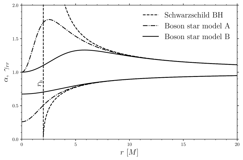
Figure 5: Comparison between the metric functions of the boson star models used in this work and those of a Schwarzschild black hole in Boyer–Lindquist coordinates. The vertical dashed line shows the position of the black hole event horizon.

Appendix B Plasma dynamics in the boson star interior

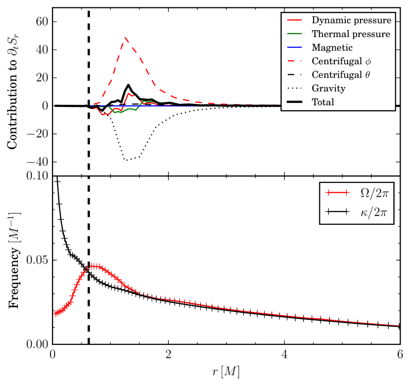
Figure 6: Top: Different contributions to the conservation equation of radial momentum (see Eq. 10) for the accretion flow onto boson star model A. Bottom: Orbital ($\Omega$) and radial epicyclic ($\kappa$) frequencies of the fluid in the boson star interior. Both plots consider time and $\phi$-averages of quantities at the equatorial plane, over the interval $t=8900-10\ 000\ M$. The vertical dashed line marks the position of the turning point of the angular velocity, $r_{\rm turn}$, so that on the left of the dashed line the flow is stable to the MRI, while on the right it is MRI unstable.

B.1 Origin of the stalled mini torus

Without an event horizon or a hard surface, a boson star also lacks a capture cross-section. As a consequence, steep centrifugal barriers appear for all angular momenta (except exactly zero) and it is possible to find stable circular orbits at all radii. Indeed, as discussed in the main text, our simulation of accretion onto boson star model A lead to the formation of a “hole”, that is, a spatial region at the centre of the boson star with very low density material and surrounded by a dense accumulation of matter in a toroidal distribution, i.e., a mini torus.

To investigate the origin of this feature, we recall that the plasma obeys the equations for local conservation of rest mass, energy, and momentum

$$\nabla_{\mu}\left(\rho u^{\mu}\right)=0\,,$$ (7)

$$\nabla_{\mu}T^{{\mu\nu}}=0\,,$$ (8)

where $\nabla_{\mu}$ denotes the covariant derivative, and $T^{{\mu\nu}}$ is the energy–momentum tensor of the fluid and the magnetic field

$$T^{\mu\nu}=\left(\rho h+b^{2}\right)u^{\mu}u^{\nu}+\left(p+b^{2}/2\right)g^{\mu\nu}-b^{\mu}b^{\nu}\,.$$ (9)

Here, $\rho$ is the rest-mass density, $h$ the fluid specific enthalpy, $p$ the thermal pressure and $b^{\mu}$ the components of the magnetic field, all measured in the fluid frame (see Porth et al., 2017). After adopting the $3+1$ decomposition of the space-time described by equation (6), it is possible to obtain an evolution equation for each component of the covariant three-momentum $S_{i}\coloneqq\gamma_{i}^{\ \mu}n^{\nu}T_{\mu\nu}$. Since accretion is best captured by the conservation of radial momentum, it is useful to group the various terms appearing in the conservation equation of $S_{r}$ and to associate with each term the corresponding physical origin. More specifically, after assuming symmetry in the $\phi$ direction and with respect to the equatorial plane, the different contributions to the evolution of $S_{r}$ can be listed as

$$\partial_{t}S_{r} =$$ (10)

Thermal pressure: $$-\partial_{r}\sqrt{\gamma}\alpha p$$

Dynamic pressure: $$-\partial_{r}\sqrt{\gamma}(\alpha v^{r}-\beta^{r})\rho h\Gamma^{2}v_{r}$$

Magnetic forces: $$-\partial_{r}\sqrt{\gamma}\{$$

$$(\alpha v^{r}-\beta^{r})[\mathbf{B}^{2}v_{r}-(B^{j}v_{j})B_{r}]$$

$$-\alpha B^{r}[(B^{j}v_{j})v_{r}+B_{r}/\Gamma^{2}]$$

$$+\alpha b^{2}/2\}$$

$$\text{Centrifugal in }\theta: +\sqrt{\gamma}\frac{1}{2}\alpha W^{\theta\theta}\partial_{r}\gamma_{\theta\theta}$$

$$\text{Centrifugal in }\phi: +\sqrt{\gamma}\frac{1}{2}\alpha W^{\phi\phi}\partial_{r}\gamma_{\phi\phi}$$

Shift: $$+\sqrt{\gamma}S_{i}\partial_{r}\beta^{i}$$

Gravity: $$+\frac{1}{2}\alpha W^{ik}\partial_{r}\gamma_{ik}-U\partial_{r}\alpha$$

$$-W^{\theta\theta}\partial_{r}\gamma_{\theta\theta}-W^{\phi\phi}\partial_{r}\gamma_{\phi\phi}\,,$$

where $\sqrt{\gamma}$ is the square root of the three-metric determinant, $B^{i}$ and $v^{i}$ are the components of the magnetic field and the fluid three-velocity, $W_{ij}\coloneqq\gamma_{i\mu}\gamma_{j\nu}T^{\mu\nu}$ those of the covariant stress tensor and $U:=n_{\mu}n_{\nu}T^{\mu\nu}$ the total energy density, all defined in the Eulerian frame. In Eq. (10), both magnetic pressure and tension are considered under the label “magnetic forces“.

The upper panel of Fig. 6, reports the numerical values of the various contributions to the conservation equation of radial momentum in Eq. 10 after averaging in time and in the $\phi$-direction. Comparing these contributions it becomes clear that the dominant term balancing gravity is the centrifugal force in $\phi$, while the evolution of radial momentum towards the equilibrium state is guided by dynamic pressure. The contribution labelled as “shift”, which results from the movement of Eulerian observers with respect to the coordinate system, is zero for the case considered here and is therefore omitted in Fig. 6.

The bottom panel of Fig. 6 shows instead the orbital ($\Omega$) and radial epicyclic ($\kappa$) frequencies – after averages in time and $\phi$-direction – of the fluid in the boson star interior. Note that while the orbital frequency is monotonically decreasing outwards in the outer parts of the flow, where it follows an essentially Keplerian fall-off, it also exhibits a local maximum and a decreasing branch as it tends to $r\to 0$. This behaviour is due to the decrease in the gravitational forces in the innermost regions of the boson star and hence to a decrease in the angular momentum needed to maintain a circular orbit. As a result, the stability criterion against the MRI, which is given by $d\Omega^{2}/dR>0$, where $R:=r\sin\theta$ (Balbus & Hawley, 1991), is fulfilled in the innermost regions of the boson star, where the MRI is essentially quenched. Under these conditions, the matter in the mini torus is unable to lose angular momentum and will be repelled by the centrifugal barrier at the radius where $d\Omega^{2}/dR=0$ and forced to move along the polar directions, where the fluid density is lower. The bottom panel of Fig. 6 also shows that this radial location coincides with the inner edge of the torus in the equatorial plane.

It is interesting to note that the conditions discussed above for the formation of the stalled torus are not met for all mini boson stars. Indeed, for a large part of the parameter space, which includes the most compact, or more relativistic, stable configurations such as the boson star model B, the rotation velocity profile of circular geodesics has no local maxima for $r>0$. As a result, the MRI is active at all radii and the plasma continues accreting down to the centre of the boson star.

Computing the angular velocity corresponding to a circular time-like geodesic for a massive particle as $\Omega:=u^{\phi}/u^{t}=[(\alpha/r)\,d\alpha/dr]^{1/2}$ (see e.g.,  Rezzolla & Zanotti, 2013), we can estimate the location of the edge of the mini torus with the corresponding turning point $r_{\rm turn}$ in the two branches for $r\to 0$ and $r\to\infty$. Similarly, we can compute the corresponding photon impact parameter at $r_{\rm turn}$ as

$$b\,(r_{\rm turn})=\frac{r_{\rm turn}}{\alpha\,(r_{\rm turn})}\,,$$ (11)

and use $b\,(r_{\rm turn})$ to estimate the radial size of the “dark region” in an accreting boson star of model A. Figure 7 shows the radius $r_{\rm turn}$ and the impact parameter $b$ for photons reaching this radius (dashed and continuous lines) for different mini boson stars, as a function of compactness (top panel) and central amplitudes of the scalar field (bottom panel). As a reference, a shadowed gray region shows the possible minimal widths for a Kerr black hole shadow, from $a=0$ to $a=1$. Also as a reference, the right axis shows the corresponding size of the dark region associated with $b$ in $\mu$as and for the case of Sgr A*. The dashed blue line corresponds to the unstable branch and the red continuous line to the stable branch of the boson star family, with the markers indicating the boson star models considered here. Overall, Fig. 7 underlines that while strong field images of boson stars with $r_{\rm turn}=0$, and hence with no central dark region, are obviously going to be drastically different from those of black holes, none of the boson stars considered here produces a dark region with size comparable to that of the black hole shadow with the same mass.

An interesting question is how general this property is amongst surfaceless and horizonless black-hole mimickers. In the discussion above, we showed that a necessary condition for the formation of the stalled mini torus, and hence of a central dark region, is the existence of a maximum in the angular velocity profile of the fluid, which – after the re-distribution of angular momentum by turbulence – follows approximately that of time-like equatorial circular geodesics. Black-hole space–times do not have maxima in such rotation profiles outside the event horizon; therefore, if the exterior space-time of the black hole mimicker is similar to that of a black hole, any maximum should occur in the interior of the object. For very compact objects with most of their mass-energy enclosed in a radius comparable to their Schwarzschild radius, the inner edge of the mini torus would then be located at an even smaller radius. In the case of slowly rotating compact objects, the (Jebsen)-Birkhoff theorem makes the above reasoning particularly relevant (Rezzolla & Zanotti, 2013).

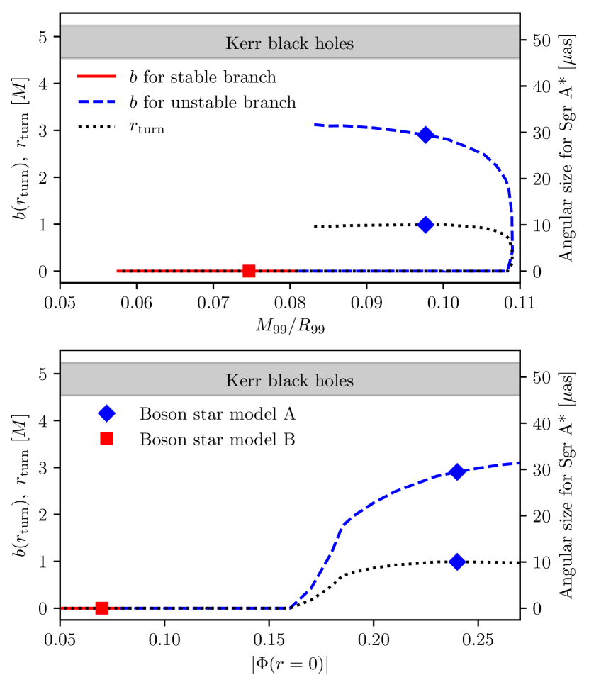
Figure 7: Radial position $r_{\rm turn}$ at which the MRI is suppressed (dotted line), and the impact parameter $b$ for photons at this radius (dashed and continuous lines) for different mini boson stars, as a function of compactness (top panel) and central amplitudes of the scalar field (bottom panel). As a reference, the shadowed gray region shows the possible minimal widths for Kerr black hole shadows. Note that all boson star models of the type considered here have dark regions that are smaller than those associated with black holes. The right axis shows the corresponding size of the dark region associated with $b$ in $\mu$as and for the case of Sgr A*. The dashed blue line corresponds to the unstable branch and the red continuous line to the stable branch of the mini boson star family. The boson star models considered in this work are indicated by markers.

B.2 Quasi-periodic oscillations

As anticipated in section 3, another peculiarity of accretion onto the boson stars is the presence of strong quasi-periodic oscillations in the mass inflow. It has been shown that for the case of black holes accreting at rates similar to those of Sgr A* and M87, the time series of the accretion rate can be used as a proxy to study the variability at the typical observing frequencies of the EHT (Porth et al., 2017). By calculating the power spectral density (PSD) of the these time series (Fig. 8), it can be observed that for the case of boson star model A the frequency peaks around $f\approx 0.04\,M^{-1}=0.002\ {\rm Hz}$, which closely corresponds to the radial epicyclic frequency $\kappa/2\pi$ at the location of the inner edge of the torus (cf. Fig. 6). The PSD reported in Fig. 8 was obtained by averaging that of $10$ not overlapping time windows in the interval $5000-10\ 000\ M$. The large amplitude of these oscillations is caused by the high density in the mini torus, which results in the displacement of a large amount of mass with every cycle. As mentioned in the main text, QPOs near the epicyclic frequency are expected from trapped p-mode oscillations that induce large excursions, both positive and negative, in the accretion rate (Rezzolla et al., 2003a, b).

Hence, a possible detection of QPOs in the mass accretion rate could provide additional means for distinguishing accreting black holes from boson stars, as we could expect the latter to show quasi-periodic oscillations at higher frequencies. In fact, for circular orbits around black holes, the epicyclic frequency decreases to zero at the innermost stable circular orbit and becomes imaginary closer to the black hole (Kato & Fukue, 1980; Abramowicz & Kluźniak, 2003).

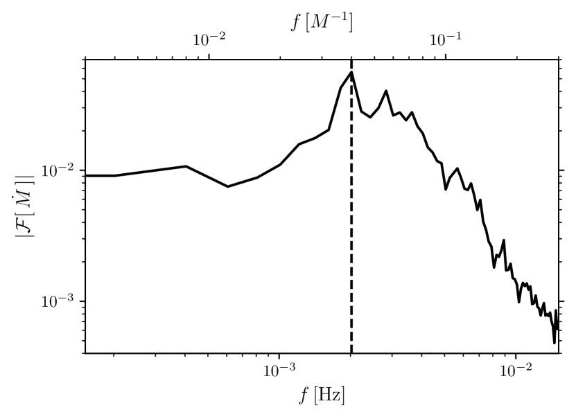
Figure 8: Power spectral density of the mass accretion rate at $r=2\,M$ for boson star model A. A peak can be observed at $f=0.002\ {\rm Hz}$, which corresponds to the radial epicyclic frequency at the inner edge of the mini torus (black dashed line).

B.3 Variability in the images of boson star model B

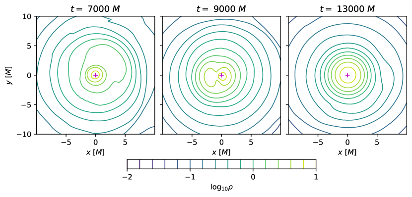
Figure 9: Isocontours of the rest-mass density for boson star model B at different times before, during, and after the absorption of the cloud discussed in Appendix B.3. The red cross marks the centre of the boson star.

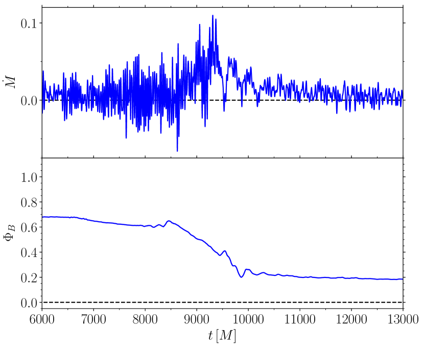
Figure 10: Same as Figure 1, showing time series of the mass and absolute magnetic flux onto boson star model B before and after the changes mentioned in Appendix B.3.

Between $t=8000\ M$ and $t=10\ 000\ M$, a series of changes in the magnetic field structure produces a drop in the absolute magnetic flux threading boson star model B (cf. Figure 1). These are caused by the absorption of an orbiting dense cloud by the central fluid structure located inside the boson star. This cloud arises from the random perturbations added to the initial condition, and it survives and grows due to non-linear interactions with the oscillating fluid structure inside the boson star. In order to ensure that the images of boson star model B obtained in the time range reported in Section 4 are representative despite this changes, we ran the simulation further until $t=13\ 000\ M$. We found that after $t=10000\ M$, the system reaches a new long-lived state in which $\Phi_{{}_{B}}$ does not have rapid changes. Figures 9 and 10 show, respectively, density isocontours and time series of the mass and magnetic flux threading the boson star before, during and after the absorption of the cloud. The images computed during the long-lived states before and after the transition, and averaged over a time window corresponding to the EHT observing time, share the features of Figures 4 and 3 that allow them to be distinguished from black hole images, namely a smaller source size and the absence of a dark region at the centre. Figure 11 shows images at the same inclinations as in Figures 4 and 3, computed over the time windows $t\in[7900\ M,9000\ M]$ and $t\in[9900\ M,11\ 000\ M]$, indicating that these image properties can indeed be considered representative of this boson star model.

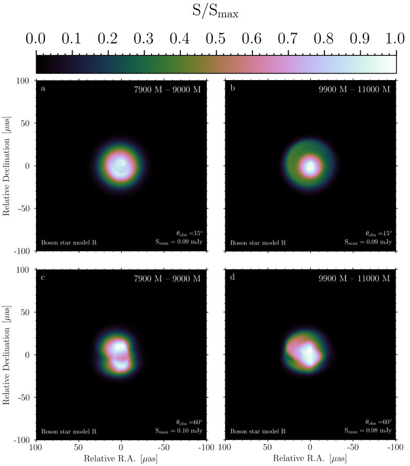
Figure 11: Ray-traced images at the same inclinations of Figures 4 (first row) and 3 (second row), averaged over the intervals $t/M\in[7900,9000]$ (left column) and $t/M\in[9900,11\ 000]$ (right column).

B.4 Time-scale for collapse

Since our simulations show that matter accreted onto the boson star keeps accumulating at its interior, a natural question that arises is for how long accretion can continue at the same rate before the accreting material reaches the critical mass to collapse to a black hole. Although an accurate answer to this question needs to take into account the non-linearity of the system, a rough estimate can be made using the accretion rate calculated in section 4 from the observed flux of Sgr A*. This calculation also ignores the effect of radiation pressure, which could contribute to slow down the accretion flow (see Zanotti et al., 2011, for the case of a Bondi–Hoyle–Littleton accretion). Assuming an upper limit on the accretion rate within a 2-sphere of radius $r=2M$ that is of the order of $10^{-6}\ {\rm M}_{\odot}\,{\rm yr}^{-1}\sim 10^{-12}\ M\,{\rm yr}^{-1}$, where the second estimate refers to Sgr A*, whose mass is $M\sim 10^{6}\,{\rm M}_{\odot}$. Considering that the scalar field in the boson stars already accounts for $\sim 90\%$ of the mass-energy contained within a radius $r=2M$, it would take $\sim 10^{11}{\rm yr}$ to accrete a sufficient amount of mass to induce a collapse to a black hole.

Clearly, such a large time-scale, which corresponds to nearly seven times the age of the Universe, suggests that the accumulation of matter in the interior of an accreting boson star, either in the form of a mini torus or of a mini cloud, may lead to the collapse to a black hole only on cosmological time-scales.

Appendix C Initial torus and development of MRI

The torus around the boson star was built according to the prescription by Abramowicz et al. (1978), which was derived for general axisymmetric metrics and is frequently employed for building tori around black holes. For the boson star case, the metric functions of the Kerr space-time were replaced by those correspondent to that of the boson star. Inside the torus, we set up a poloidal magnetic loop from a vector potential following density isosurfaces, $A_{\phi}\propto\max((\rho/\rho_{\mathrm{max}}-0.2),0)$. We adopted the following actions in order to make the comparison between the simulated accretion flows as close as possible:

1. Using the bisection method, the value of the constant angular momentum of the tori was set in such way that they shared the same inner (outer) radius of $6\,(42)\,M$.

2. We normalized the rest-mass density such that in each case it took the maximum value $\rho_{\rm max}=1$.

3. We rescaled the magnetic field so that the ratio of gas to magnetic pressure had a minimum of $\beta_{\rm min}=11.2$.

The simulations were performed in polar coordinates on a grid logarithmically spaced in the radial direction. We employed three levels of adaptive mesh refinement triggered by the Löhner scheme (Löhner, 1987), to give an effective resolution of $\{N_{r},N_{\theta},N_{\phi}\}\simeq\{512,128,128\}$, and with the outer boundary placed at $1000\,M$, thus with a radial-grid spacing of $0.19\,M$ at the inner edge of the torus. The accretion torus was perturbed to trigger the MRI, causing turbulent transport of angular momentum and driving the accretion (Balbus & Hawley, 1991). To ensure the ability to resolve the MRI, the resolution employed is comparable to those encountered in the literature for simulations of accretion onto black holes (see e.g.,  Narayan et al., 2012; Mościbrodzka et al., 2016; Mizuno et al., 2018). As customary, we have computed the MRI quality factor $Q_{\rm MRI}$ (see Sano et al., 2004; Noble et al., 2010; McKinney et al., 2012), making sure that $Q_{\rm MRI}\gtrsim 6$ in the relevant regions (Fig. 12), which ensures that the correct saturation values of the shear stress and the ratio between magnetic and fluid pressure are achieved (Sano et al., 2004).

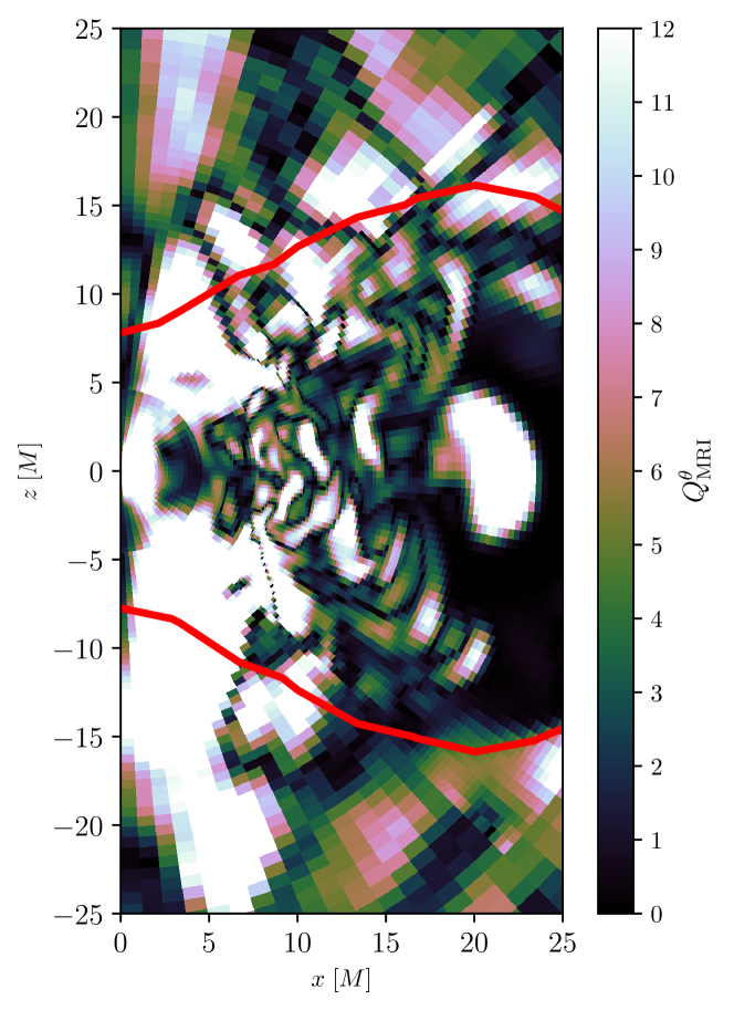
Figure 12: MRI quality factor $Q_{\rm MRI}$ for boson star model B at $t=1000\ M$, when the instability is developing. The red contour indicates the edges of the torus, approximated as the contour in which density falls to 1% of the maximum density of the original torus. It can be seen that $Q_{\rm MRI}\gtrsim 6$ where the instability is developing.

References

- Abdujabbarov et al. (2015) Abdujabbarov A. A., Rezzolla L., Ahmedov B. J., 2015, Mon. Not. R. Astron. Soc., 454, 2423
- Abramowicz & Kluźniak (2003) Abramowicz M. A., Kluźniak W., 2003, Gen. Relativ. Gravit., 35, 69
- Abramowicz et al. (1978) Abramowicz M., Jaroszynski M., Sikora M., 1978, Astron. Astrophys., 63, 221
- Abuter et al. (2018a) Abuter R., et al., 2018a, Astron. Astrophys., 615, L15
- Abuter et al. (2018b) Abuter R., et al., 2018b, Astron. Astrophys., 618, L10
- Abuter et al. (2020) Abuter R., et al., 2020, Astronomy & Astrophysics, 636, L5
- Akiyama et al. (2015) Akiyama K., et al., 2015, Astrophys. J., 807, 150
- Albrecht & Steinhardt (1982) Albrecht A., Steinhardt P. J., 1982, Physical Review Letters, 48, 1220
- Amaro-Seoane et al. (2010) Amaro-Seoane P., Barranco J., Bernal A., Rezzolla L., 2010, JCAP, 11, 002
- Anderson & Brill (1997) Anderson P. R., Brill D. R., 1997, Phys. Rev. D, 56, 4824
- Arvanitaki et al. (2010) Arvanitaki A., Dimopoulos S., Dubovsky S., Kaloper N., March-Russell J., 2010, Phys. Rev. D, 81, 123530
- Balbus & Hawley (1991) Balbus S. A., Hawley J. F., 1991, Astrophys. J., 376, 214
- Bezares et al. (2017) Bezares M., Palenzuela C., Bona C., 2017, Phys. Rev. D, 95, 124005
- Blandford & Znajek (1977) Blandford R. D., Znajek R. L., 1977, Mon. Not. R. Astron. Soc., 179, 433
- Boehle et al. (2016) Boehle A., et al., 2016, Astrophys. J., 830, 17
- Brill & Hartle (1964) Brill D. S., Hartle J., 1964, Phys. Rev., 135, B271
- Broderick et al. (2009) Broderick A. E., Loeb A., Narayan R., 2009, The Astrophysical Journal, 701, 1357
- Capozziello et al. (2000) Capozziello S., Lambiase G., Torres D. F., 2000, Class. Quant. Grav., 17, 3171
- Cardoso et al. (2008) Cardoso V., Pani P., Cadoni M., Cavaglià M., 2008, Phys. Rev. D, 77, 124044
- Cardoso et al. (2016) Cardoso V., Franzin E., Pani P., 2016, Phys. Rev. Lett., 116, 171101
- Cattoen et al. (2005) Cattoen C., Faber T., Visser M., 2005, Class. Quantum Grav., 22, 4189
- Chael et al. (2016) Chael A. A., Johnson M. D., Narayan R., Doeleman S. S., Wardle J. F. C., Bouman K. L., 2016, Astrophys. J., 829, 11
- Chatzopoulos et al. (2015) Chatzopoulos S., Fritz T. K., Gerhard O., Gillessen S., Wegg C., Genzel R., Pfuhl O., 2015, Mon. Not. R. Astron. Soc., 447, 948
- Chirenti & Rezzolla (2008) Chirenti C. B. M. H., Rezzolla L., 2008, Phys. Rev. D, 78, 084011
- Chirenti & Rezzolla (2016) Chirenti C., Rezzolla L., 2016, Phys. Rev. D, 94, 084016
- Comins & Schutz (1978) Comins N., Schutz B., 1978, Proceedings Of The Royal Society Of London A Mathematical And Physical Sciences, 364, 211
- Cunha et al. (2015) Cunha P. V. P., Herdeiro C. A. R., Radu E., Rúnarsson H. F., 2015, Phys. Rev. Lett., 115, 211102
- Cunha et al. (2017a) Cunha P. V. P., Font J. A., Herdeiro C., Radu E., Sanchis-Gual N., Zilhão M., 2017a, Phys. Rev. D, 96, 104040
- Cunha et al. (2017b) Cunha P. V. P., Berti E., Herdeiro C. A. R., 2017b, Phys. Rev. Lett., 119, 251102
- Cunningham & Bardeen (1973) Cunningham C. T., Bardeen J. M., 1973, Astrophys. J., 183, 237
- Dabrowski & Schunck (2000) Dabrowski M. P., Schunck F. E., 2000, Astrophys. J., 535, 316
- Doeleman et al. (2008) Doeleman S. S., et al., 2008, Nature, 455, 78
- EHTC (2019a) Event Horizon Telescope Collaboration et al., 2019a, Astrophys. J. Lett., 875, L1
- EHTC (2019b) Event Horizon Telescope Collaboration et al., 2019b, Astrophys. J. Lett., 875, L2
- EHTC (2019c) Event Horizon Telescope Collaboration et al., 2019c, Astrophys. J. Lett., 875, L3
- EHTC (2019d) Event Horizon Telescope Collaboration et al., 2019d, Astrophys. J. Lett., 875, L4
- EHTC (2019e) Event Horizon Telescope Collaboration et al., 2019e, Astrophys. J. Lett., 875, L5
- EHTC (2019f) Event Horizon Telescope Collaboration et al., 2019f, Astrophys. J. Lett., 875, L6
- Falcke et al. (2000) Falcke H., Melia F., Agol E., 2000, Astrophys. J. Lett., 528, L13
- Fish et al. (2016) Fish V. L., et al., 2016, Astrophys. J., 820, 90
- Fujii & ichi Maeda (2003) Fujii Y., ichi Maeda K., 2003, Classical and Quantum Gravity, 20, 4503
- Ghez et al. (2008) Ghez A. M., et al., 2008, Astrophys. J., 689, 1044
- Gillessen et al. (2009) Gillessen S., Eisenhauer F., Fritz T. K., Bartko H., Dodds-Eden K., Pfuhl O., Ott T., Genzel R., 2009, Astrophys. J. Lett., 707, L114
- Goddi et al. (2017) Goddi C., et al., 2017, International Journal of Modern Physics D, 26, 1730001
- Grenzebach (2016) Grenzebach A., 2016, The Shadow of Black Holes. Springer International Publishing, Cham doi:10.1007/978-3-319-30066-5
- Grould et al. (2017) Grould M., Meliani Z., Vincent F. H., Grandclément P., Gourgoulhon E., 2017, Classical and Quantum Gravity, 34, 215007
- Guzmán (2004) Guzmán F. S., 2004, Physical Review D - Particles, Fields, Gravitation and Cosmology, 70, 10
- Guzmán (2005) Guzmán F. S., 2005, Journal of Physics: Conference Series, 24, 241
- Guzmán (2006) Guzmán F. S., 2006, Phys. Rev. D, 73, 021501
- Guzmán (2011) Guzmán F. S., 2011, Journal of Physics: Conference Series, 314, 012085
- Hui et al. (2017) Hui L., Ostriker J. P., Tremaine S., Witten E., 2017, Phys. Rev. D, 95, 043541
- Hunter (2007) Hunter J. D., 2007, Computing In Science & Engineering, 9, 90
- Issaoun et al. (2019) Issaoun S., et al., 2019, Astrophys. J., 871, 30
- Johnson & Gwinn (2015) Johnson M. D., Gwinn C. R., 2015, Astrophys. J., 805, 180
- Kato & Fukue (1980) Kato S., Fukue J., 1980, Publications of the Astronomical Society of Japan, 32, 377
- Kaup (1968) Kaup D. J., 1968, Phys. Rev., 172, 1331
- Kleihaus et al. (2005) Kleihaus B., Kunz J., List M., 2005, Phys. Rev., D72, 064002
- Kleihaus et al. (2012) Kleihaus B., Kunz J., Schneider S., 2012, Phys. Rev. D, 85, 024045
- Kramer et al. (2004) Kramer M., Backer D. C., Cordes J. M., Lazio T. J. W., Stappers B. W., Johnston S., 2004, New Astron. Rev., 48, 993
- Liebling & Palenzuela (2012) Liebling S. L., Palenzuela C., 2012, Living Reviews in Relativity, 15, 6
- Linde (1982) Linde A., 1982, Physics Letters B, 108, 389
- Liu et al. (2012) Liu K., Wex N., Kramer M., Cordes J. M., Lazio T. J. W., 2012, Astrophys. J., 747, 1
- Löhner (1987) Löhner R., 1987, Computer Methods in Applied Mechanics and Engineering, 61, 323
- Marrone et al. (2006) Marrone D. P., Moran J. M., Zhao J.-H., Rao R., 2006, Astrophys. J., 640, 308
- Marrone et al. (2007) Marrone D. P., Moran J. M., Zhao J.-H., Rao R., 2007, Astrophys. J.l, 654, L57
- Matos & Guzman (2000) Matos T., Guzman F. S., 2000, Class. Quant. Grav., 17, L9
- Mazur & Mottola (2004) Mazur P. O., Mottola E., 2004, Proceedings of the National Academy of Science, 101, 9545
- McKinney et al. (2012) McKinney J. C., Tchekhovskoy A., Blandford R. D., 2012, Mon. Not. R. Astron. Soc., 423, 3083
- Meliani et al. (2016) Meliani Z., Grandclément P., Casse F., Vincent F. H., Straub O., Dauvergne F., 2016, Classical and Quantum Gravity, 33, 155010
- Mizuno et al. (2018) Mizuno Y., et al., 2018, Nature Astronomy, 2, 585
- Mościbrodzka et al. (2009) Mościbrodzka M., Gammie C. F., Dolence J. C., Shiokawa H., Leung P. K., 2009, Astrophys. J., 706, 497
- Mościbrodzka et al. (2016) Mościbrodzka M., Falcke H., Shiokawa H., 2016, Astron. Astrophys., 586, A38
- Narayan et al. (2012) Narayan R., Sa̧dowski A., Penna R. F., Kulkarni A. K., 2012, Mon. Not. R. Astron. Soc., 426, 3241
- Noble et al. (2010) Noble S. C., Krolik J. H., Hawley J. F., 2010, The Astrophysical Journal, 711, 959
- Oliphant (2006) Oliphant T., 2006, Guide to NumPy, Continuum Press, Austin
- Olivares et al. (2019) Olivares H., Porth O., Davelaar J., Most E. R., Fromm C. M., Mizuno Y., Younsi Z., Rezzolla L., 2019, Astronomy & Astrophysics, 629, A61
- Palenzuela et al. (2017) Palenzuela C., Pani P., Bezares M., Cardoso V., Lehner L., Liebling S., 2017, Phys. Rev. D, 96, 104058
- Porth et al. (2017) Porth O., Olivares H., Mizuno Y., Younsi Z., Rezzolla L., Moscibrodzka M., Falcke H., Kramer M., 2017, Computational Astrophysics and Cosmology, 4, 1
- Preskill et al. (1983) Preskill J., Wise M. B., Wilczek F., 1983, Physics Letters B, 120, 127
- Psaltis et al. (2015a) Psaltis D., Narayan R., Fish V. L., Broderick A. E., Loeb A., Doeleman S. S., 2015a, Astrophys. J., 798, 15
- Psaltis et al. (2015b) Psaltis D., Özel F., Chan C.-K., Marrone D. P., 2015b, Astophys. J., 814, 115
- Psaltis et al. (2016) Psaltis D., Wex N., Kramer M., 2016, Astrophys. J., 818, 121
- Rezzolla & Zanotti (2013) Rezzolla L., Zanotti O., 2013, Relativistic Hydrodynamics. Oxford University Press, Oxford, UK, doi:10.1093/acprof:oso/9780198528906.001.0001
- Rezzolla et al. (2003a) Rezzolla L., Yoshida S., Zanotti O., 2003a, Mon. Not. R. Astron. Soc., 344, 978
- Rezzolla et al. (2003b) Rezzolla L., Yoshida S., Maccarone T. J., Zanotti O., 2003b, Mon. Not. R. Astron. Soc., 344, L37
- Roelofs et al. (2019) Roelofs F., et al., 2019, Astron. Astrophys., 625, A124
- Ruffini & Bonazzola (1969) Ruffini R., Bonazzola S., 1969, Phys. Rev., 187, 1767
- Sanchis-Gual et al. (2019) Sanchis-Gual N., Di Giovanni F., Zilhão M., Herdeiro C., Cerdá-Durán P., Font J. A., Radu E., 2019, Phys. Rev. Lett., 123, 221101
- Sano et al. (2004) Sano T., Inutsuka S.-i., Turner N. J., Stone J. M., 2004, Astrophys. J., 605, 321
- Saxton et al. (2016) Saxton C. J., Younsi Z., Wu K., 2016, Mon. Not. R. Astron. Soc., 461, 4295
- Schunck & Liddle (1997) Schunck F. E., Liddle A. R., 1997, Phys. Lett., B404, 25
- Schunck & Mielke (1999) Schunck F. E., Mielke E. W., 1999, General Relativity and Gravitation, 31, 787
- Schunck & Torres (2000) Schunck F. E., Torres D. F., 2000, Int. J. Mod. Phys., D9, 601
- Seidel & Suen (1990) Seidel E., Suen W.-M., 1990, Phys. Rev. D, 42, 384
- Seidel & Suen (1991) Seidel E., Suen W.-M., 1991, Phys. Rev. Lett., 66, 1659
- Shakura & Sunyaev (1973) Shakura N. I., Sunyaev R. A., 1973, Astron. Astrophys., 24, 337
- Torres et al. (2000) Torres D. F., Capozziello S., Lambiase G., 2000, Phys. Rev. D, 62, 104012
- Ureña-López (2002) Ureña-López L. A., 2002, Classical and Quantum Gravity, 19, 2617
- Vincent et al. (2016) Vincent F. H., Meliani Z., Grandclement P., Gourgoulhon E., Straub O., 2016, Class. Quant. Grav., 33, 105015
- Virbhadra & Ellis (2000) Virbhadra K. S., Ellis G. F. R., 2000, Phys. Rev., D62, 084003
- Virbhadra et al. (1998) Virbhadra K. S., Narasimha D., Chitre S. M., 1998, Astron. Astrophys., 337, 1
- Wang et al. (2004) Wang Z., Bovik A. C., Sheikh H. R., Simoncelli E. P., 2004, IEEE Transactions on Image Processing, 13, 600
- Wex & Kopeikin (1999) Wex N., Kopeikin S., 1999, Astrophys. J., 514, 388
- Wheeler (1955) Wheeler J. A., 1955, Phys. Rev., 97, 511
- Yoshida & Eriguchi (1996) Yoshida S., Eriguchi Y., 1996, Mon. Not. R. Astron. Soc., 282, 580
- Younsi et al. (2012) Younsi Z., Wu K., Fuerst S. V., 2012, Astron. Astrophys., 545, A13
- Younsi et al. (2016) Younsi Z., Zhidenko A., Rezzolla L., Konoplya R., Mizuno Y., 2016, Phys. Rev. D, 94, 084025
- Younsi et al. (2020) Younsi Z., Porth O., Mizuno Y., Fromm C. M., Olivares H., 2020, Proceedings of the International Astronomical Union, 14, 9
- Zanotti et al. (2011) Zanotti O., Roedig C., Rezzolla L., Del Zanna L., 2011, Mon. Not. R. Astron. Soc., 417, 2899