Abstract

Methods based on Bayesian decision tree ensembles have proven valuable in constructing high-quality predictions, and are particularly attractive in certain settings because they encourage low-order interaction effects. Despite adapting to the presence of low-order interactions for prediction purpose, we show that Bayesian decision tree ensembles are generally anti-conservative for the purpose of conducting interaction detection. We address this problem by introducing Dirichlet process forests (DP-Forests), which leverage the presence of low-order interactions by clustering the trees so that trees within the same cluster focus on detecting a specific interaction. We show on both simulated and benchmark data that DP-Forests perform well relative to existing interaction detection techniques for detecting low-order interactions, attaining very low false-positive and false-negative rates while maintaining the same performance for prediction using a comparable computational budget.

1 INTRODUCTION

In many scientific problems, a primary goal is to discover structures which allow the problem to be described parsimoniously. For example, one may wish to find a small subset of candidate variables that are predictive of a response of interest; this structure is referred to as sparsity. Another structure is interaction (or additive) structure. An extreme case of additive structure is a generalized additive model (see, e.g., Hastie,, 2017), where the effects of the predictors combine additively without any interactions. Teasing out additive structures can be valuable because it can substantially simplify the interpretation of a model. For example, if a given predictor does not interact with other predictors then it can be interpreted in isolation without reference to the values of other predictors. When predictors do interact, interpretation of the interactions is typically simplified whenever the interactions are of low-order. We consider the nonparametric regression problem $Y_{i}=f_{0}(X_{i})+\epsilon_{i}$, $\epsilon_{i}\sim\operatorname{Normal}(0,\sigma^{2})$, where $Y_{i}$ is a response of interest and $X_{i}\in\mathbb{R}^{P}$ is a vector of predictors, however the methods we develop here can be easily extended to many other settings. The variables $x_{j}$ and $x_{k}$ are said to interact if $f_{0}(x)$ cannot be written as $f_{0}(x)=f_{0\backslash j}(x)+f_{0\backslash k}(x)$ where $f_{0\backslash j}$ and $f_{0\backslash k}$ do not depend on $x_{j}$ and $x_{k}$ respectively. One can define higher order interactions similarly: a group of $K$ variables is said to have a $K$-way interaction if $f_{0}(x)$ cannot be decomposed as a sum of $K$ or fewer functions, each of which depends on fewer than $K$ of the variables.

Methods which estimate $f_{0}(x)$ using an ensemble of Bayesian decision trees have proven useful in a number of statistical problems. Beginning with the seminal work of Chipman et al., (2010), Bayesian additive regression trees (BART) have been successfully applied in a diverse range of settings including survival analysis (Sparapani et al.,, 2016), causal inference (Hahn et al.,, 2017), variable selection in high dimensional settings (Linero,, 2016; Bleich et al.,, 2014), loglinear models (Murray,, 2017), and analysis of functional data (Starling et al.,, 2018). A key motivating factor for the use of BART is precisely that it is designed to taking advantage of low-order interactions in the data. Indeed, Linero and Yang, (2017) and Rockova and van der Pas, (2017) illustrate theoretically that the presence of low-order interactions is precisely the type of structure which BART excels at capturing. Hence BART appears to be an ideal tool for extracting low-order and potentially non-linear interactions.

Surprisingly, we show that, despite the ability of BART to capture low-order interactions for prediction purposes, it is nonetheless not suitable for conducting fully-Bayesian inference for the selection task of interaction detection. When taken at face value as a Bayesian model, we show empirically that BART generally leads to the detection of spurious interaction effects. This is not contradictory because optimal prediction accuracy is generally not sufficient to guarantee consistency in variable selection (see, e.g., Wang et al.,, 2007).

We discuss the general problem which leads to the detection of spurious interactions; while this development is couched in the BART framework, we believe that the fundamental issues also occur for other decision tree ensembling methods. Specifically, the problem is that there is no penalty associated to including spurious interaction terms in the model. We then introduce a suitable modification to the BART framework which addresses this problem and allows BART detect interactions in a fully-Bayesian fashion. We accomplish this by clustering the trees into non-overlapping groups. Intuitively, the shallow trees comprising each cluster work together to learn a single low-order interaction. To bypass the need to specify the number of clusters, we induce the clustering through a Dirichlet process prior (Ferguson,, 1973). We refer to the ensemble constructed in this fashion as a Dirichlet Process Forest (DP-Forest).

1.1 A Simple Example

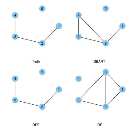
Figure 1: The interaction structure detected in the example from Section 1.1. “Truth” denotes the true interaction structure in the example.

To motivate the problem, we consider a simulated data example of Vo and Pati, (2016). This example takes $P=100$, $N=100$, $X_{i}\sim\operatorname{Normal}(\bm{0},0.02\,\mathrm{I})$, and $f_{0}(x)=x_{1}+x_{2}^{2}+x_{3}+x_{4}^{2}+x_{5}+x_{1}x_{2}+x_{2}x_{3}+x_{3}x_{4}$. We compare the DP-Forest we propose to a variant of BART referred to as SBART (Linero and Yang,, 2017) which can accommodate sparsity in variable selection. We also consider the recently proposed iterative random forests algorithm of Basu et al., (2018), selecting interactions whose stability score is higher than 0.5. In Figure 1 we display the interaction structure detected by each method on this data; while we considered only one iteration of this experiment here, these results are typical of replications of the experiment.

Here, SBART detects a spurious edge between $x_{2}$ and $x_{4}$. This occurs because BART, despite its fundamentally additive nature, does not include any penalization which discourages unnecessary interactions from being included. On the contrary, BART expect interactions to occur between relevant predictions; considering a draw from a BART prior such that $x_{2}$ and $x_{4}$ are included in the model, an interaction between these variables is a-priori likely. Adapting Bayesian decision tree ensembles to interaction detection then requires a prior which discourages the inclusion of weak interactions. The iRF similarly detects two spurious interactions and misses a relevant interaction between $x_{3}$ and $x_{4}$.

1.2 Related Work

Recent work has studied the theoretical properties of BART. Linero and Yang, (2017) and Rockova and van der Pas, (2017) show that certain variants of BART are capable of adaptively attaining near-minimax-optimal rates of posterior concentration when $f_{0}$ can be expressed as a sum of low-order interaction terms $f_{0}(x)=\sum_{v=1}^{V}f_{0v}(x)$ with each $f_{0v}(x)$ depending on a small subset of $\mathcal{S}_{v}$ of the predictors. In view this, one might conclude that no modification to BART is needed. This is true if one cares only about the mean integrated squared error $\int(f_{0}(x)-f(x))^{2}\,F_{0}(dx)$ where $X_{i}\stackrel{{\scriptstyle\text{iid}}}{{\sim}}F_{0}$. Optimal prediction performance, however, does not imply that variable selection and interaction detection are being performed adequately. If $\mathcal{S}_{0}$ is the true interaction structure of the data $\mathcal{S}$ is an estimate of $\mathcal{S}_{0}$, then attaining the minimax estimation rate for $f_{0}$ in terms of prediction error typically only guarantees that $\mathcal{S}_{0}\subseteq\mathcal{S}$ (not $\mathcal{S}\subseteq\mathcal{S}_{0}$).

Several other methods have been recently proposed in the literature specifically for the task of interaction detection. We offer a non-comprehensive review. For a recent review, see Bien et al., (2013). Lim and Hastie, (2015) proposed a hierarchical group-lasso which enforces the constraint that the presence of a given interaction implies the presence of the associated main effects; a similar approach is given by Bien et al., (2013). A potential shortcoming of these approaches is that they focus on linear models and allow only pairwise interactions. Radchenko and James, (2010) propose the VANISH algorithm, which allows for nonlinear effects through the use of basis function expansions, but again limits to pairwise interactions. Several decision-tree based methods have also been proposed. The additive groves procedure of Sorokina et al., (2008) uses an adaptive boosting-type algorithm to sequentially test for the presence of interactions between variables after performing a variable screening step. Basu et al., (2018) propose the iterative random forest (iRF) algorithm which flags “stable” interaction effects as those which appear consistently in many trees in a certain random forest.

2 BAYESIAN TREE ENSEMBLES

2.1 The BART Prior

Our starting point is the Bayesian additive regression trees (BART) framework of Chipman et al., (2010), which treats the function $f_{0}(\cdot)$ as the realization of a sum of random decision trees

$$f(x)=\sum_{t=1}^{T}g(x;\mathcal{T}_{t},\mathcal{M}_{t}),$$

where $\mathcal{T}_{t}$ denotes the tree structure (including the decision rules) of the $t^{\text{th}}$ tree and $\mathcal{M}_{t}=\{\mu_{t\ell}:\ell\in\mathcal{L}_{t}\}$ denotes the parameters associated to the leaf nodes; here, $\mathcal{L}_{t}$ denotes the collection of leaf nodes of $\mathcal{T}_{t}$. Let $[x\leadsto(t,\ell)]$ denote the event that the point $x$ is associated to leaf $\ell$ in tree $t$. The function $g(x;\mathcal{T}_{t},\mathcal{M}_{t})$ then returns $\mu_{t\ell}$ whenever $[x\leadsto(t,\ell)]$ occurs.

We follow Chipman et al., (2010) and specify a branching process prior for the tree structure $\mathcal{T}_{t}$. A sample from the prior for $\mathcal{T}_{t}$ is generated iteratively, starting from a tree with a single node of depth $d=0$; this is made a branch with two children with probability $q(d)=\gamma/(1+\beta)^{d}$, and is made a leaf node otherwise. We repeat this process independently for all nodes of depth $d=1,2,\ldots$ until all nodes at depth $d$ are leaves. After the structure of the tree is generated, each branch $b$ is associated with a decision rule of the form $[x_{j}\leq C_{b}]$. The coordinate $j$ used to construct the decision rule is sampled with probability $s_{j}$ where $s=(s_{1},\ldots,s_{P})$ is a probability vector. The splitting proportion $s$ will play a key role later as an avenue for inducing sparsity in the regression function. Finally, we generate $C_{b}\sim\operatorname{Uniform}(L_{j},U_{j})$ where $(L_{1},U_{1})\times\cdots\times(L_{P},U_{P})$ is the hyper-rectangle corresponding to the values of $x$ that lead to branch $b$. We remark that this choice for $C_{b}$ differs from the scheme used by other BART implementations; we adopt it to simplify the full conditionals we derive in Section 3.

For the prior on $\mathcal{M}_{t}$ we set $\mu_{t\ell}\stackrel{{\scriptstyle\text{iid}}}{{\sim}}\operatorname{Normal}(0,\sigma^{2}_{\mu}/T)$ conditional on $\mathcal{T}_{t}$ and $\sigma^{2}_{\mu}$. By taking the variance to be $\sigma_{\mu}^{2}/T$ we ensure that the prior level of signal is constant as $T$ increases. The normal prior is selected for its conjugacy; we note, however, that any prior for $\mu_{t\ell}$ with mean $0$ and variance $\sigma_{\mu}/T$ leads to the approximation $f(x)\sim\operatorname{Normal}(0,\sigma^{2}_{\mu})$ by the central limit theorem. We fix $\beta=2$ and $\gamma=0.95$; we refer readers to Linero and Yang, (2017) for further details regarding prior specification, and to Chipman et al., (2013) and Linero, (2017) for detailed reviews of Bayesian decision tree methods.

2.2 Leveraging Structural Information

Several recent developments have extended the BART methodology to take advantage of structural information. Linero, (2016) noted that sparsity in $f_{0}(x)$ can be accommodated automatically by setting $s\sim\operatorname{Dirichlet}(\alpha/P,\ldots,\alpha/P)$. Recall here that $s_{j}$ denotes the prior probability that, for a fixed branch, coordinate $j$ will be used to construct a split at a that branch. Hence, if $s$ is nearly-sparse with $d$ non-sparse entries, the prior will encourage realizations from the prior to include only the $d$ predictors with non-sparse entries. Linero and Yang, (2017) showed that this prior for $s$ induces highly desirable posterior concentration properties; in particular, the posterior of $f(x)$ concentrates at close to the oracle minimax rate if we had known the relevant predictors beforehand.

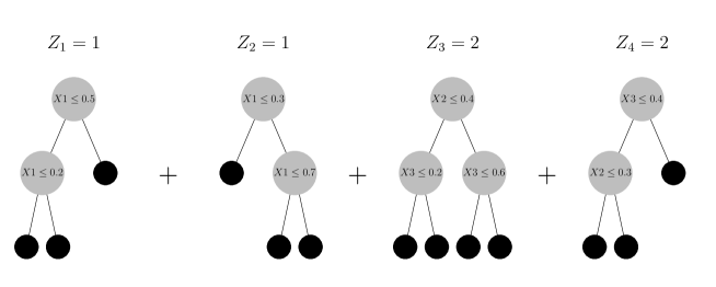
Figure 2: Schematic showing the effect of clustering trees within the ensemble. When $Z_{t}=1$ split are constructed with $X_{1}$, but when $Z_{t}=2$ splits are constructed with $(X_{2},X_{3})$.

Linero and Yang, (2017) also introduce the SBART model, which uses soft decision trees (Irsoy et al.,, 2012) which effectively replace the decision boundaries of BART with smooth sigmoid functions. This allows the SBART model to adapt to the smoothness level of $f(x)$; consequently, if $f_{0}(x)$ is assumed to be $\alpha$-Hölder, the posterior for the SBART model concentrates around $f_{0}(x)$ at close to the oracle minimax rate obtainable when the smoothness level is known a-priori. While the methodology we develop applies to the usual BART models, we will use the SBART model with the sparsity-inducing Dirichlet prior in all of our illustrations.

3 DP-FORESTS

The distribution of $(\mathcal{T}_{t},\mathcal{M}_{t})$ in the BART model is parameterized by the splitting proportions $s$, leaf variance $\sigma^{2}_{\mu}$, and tree topology parameters $(\gamma,\beta)$. To encourage a small number of low-order interactions, we specify a prior which clusters the trees into non-overlapping groups such that each cluster constructs splits using different subsets of the predictors. A schematic is given in Figure 2 with $T=4$. In this figure we see that the first two trees are dedicated to learning a main effect for $x_{1}$ while the second two trees are dedicated to learning an interaction between $x_{2}$ and $x_{3}$.

We induce a clustering by using tree-specific splitting proportions $s^{(t)}\sim G$ and using a Dirichlet process prior on $G$ (Ferguson,, 1973). Specifically, we let $s^{(t)}\stackrel{{\scriptstyle\text{iid}}}{{\sim}}G$ conditional on $G$ and let $G\sim\operatorname{DP}(\omega G_{0})$ where $G_{0}$ is a $\operatorname{Dirichlet}(\alpha w_{1},\ldots,\alpha w_{P})$ distribution and $\omega$ denotes the precision parameter of the Dirichlet process. Using the latent-cluster interpretation of the Dirichlet process (see, .e.g, Teh et al.,, 2006) this can be approximated by the following generative model:

1. Draw $\pi\sim\operatorname{Dirichlet}(\omega/K,\ldots,\omega/K)$ for large $K$.

2. Draw $Z_{1},\ldots,Z_{T}\stackrel{{\scriptstyle\text{ind}}}{{\sim}}\operatorname{Categorical}(\pi)$.

3. Draw $s^{(1)},\ldots s^{(K)}\stackrel{{\scriptstyle\text{ind}}}{{\sim}}\operatorname{Dirichlet}(\alpha w_{1},\ldots,\alpha w_{P})$ where $\sum_{p=1}^{P}w_{p}=1,w_{p}\geq 0$.

4. For $t=1,\ldots,T$, draw $(\mathcal{T}_{t},\mathcal{M}_{t})$ as described in Section 2 with $s=s^{(Z_{t})}$.

The $Z_{t}$’s cluster trees such that the trees within each group capture a single low-order interaction. Note that the use of the the sparsity inducing prior in step 3 above ensures that each $s^{(k)}$ will be nearly-sparse, and hence the trees with $Z_{t}=k$ will split on only a small subset of the predictors. The role played by this weight vector $w$ is to encourage a subset of the predictors to appear in multiple different interactions. For example, if there are interactions $(X_{1},X_{2})$ and $(X_{2},X_{3})$ we do not want to encourage an additional $(X_{1},X_{3})$ interaction. A large value of $w_{2}$ allows for this by encouraging $X_{2}$ to appear in several interactions.

3.1 Properties of the Prior

The degree of sparsity within each cluster of trees, as well as the overall number of clusters used, are determined by the hyperparameters $\alpha$ and $\omega$. These hyperparameters are key in determining the interaction structures that the prior favors. To help anchor intuition we first consider several special cases of the DP-Forests model. First, we consider the behavior of the prior as $\alpha\to 0$ with $\omega$ fixed. In this case, with high probability each $s^{(t)}$ will have only one non-sparse entry. Consequently, each tree in the ensemble will split on at most one predictor. Because the trees are composed additively, this implies that none of the variables interact, and hence the prior concentrates on a sparse generalized additive model (SPAM, Ravikumar et al.,, 2007). On the other hand, as $\alpha\to\infty$ we see that $s^{(t)}\to(w_{1},\ldots,w_{P})$ so that the prior reverts to original BART model with splitting proportions given by $(w_{1},\ldots,w_{P})$ described by Bleich et al., (2014).

We can conduct a similar analysis with $\alpha$ fixed and $\omega$ with $K\to\infty$. As $\omega\to\infty$, each tree will be associated to a unique $s^{(t)}$. As $\omega\to 0$, on the other hand, all of the trees share the same $s^{(t)}$ so that the model collapses to the Dirichlet additive regression trees model described by Linero, (2016).

The key difference between BART and a DP-Forest is that, once two variables are included, BART does not penalize interactions. Let $A_{i}$ and $A_{j}$ denote the event that variable $i$ and $j$ are included in the model, let $A_{ij}$ denote the event that variables $i$ and $j$ interact, and let $\Pi_{\alpha,\omega}$ denote the joint prior distribution for $\mathcal{T}_{1},\ldots,\mathcal{T}_{T}$. We study the prior on the interaction structure by examining the probabilities $\Lambda(\alpha,\omega)=\Pi_{\alpha,\omega}(A_{ij}\mid A_{i}\cap A_{j}),$ and $\Xi(\alpha,\omega)=\Pi_{\alpha,\omega}(A_{ik}\mid A_{ij}\cap A_{kj}).$ In words, $\Lambda$ is the probability that $(i,j)$ interact given that both variables are relevant, while $\Xi$ represents the probability that $(i,k)$ interact given that $(i,j)$ and $(k,j)$ interact. Additionally, we examine the relationship between the average number of two-way interactions included in the model and the number of variables included.

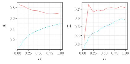
Figure 3: Plots of various quantities for $\omega=0$ (solid, corresponding to SBART) and $\omega=1$ (dashed) with $P=5$ and $T=50$. Left: plot of $\alpha$ against $\Lambda$. Middle: Plot of $\alpha$ against $\Xi$. Right: plot of the number of variables included in the model against the number of interactions.

Figure 3 shows several relationships between these quantities as $\alpha$ varies for both SBART and DP-Forests. We see that $\Lambda$ is quite large for all values of $\alpha$ with SBART, implying that the prior expects any variables included in the model to interact; the trend is decreasing in $\alpha$ only because a larger number of predictors will be included in the model, causing variables to compete for branches in the ensemble. DP-Forests do not encourage the inclusion of interactions, particularly when $\alpha$ is small. Next, we see that $\Xi$ is also uniformly large for SBART. This implies that the prior does not encourage interaction structures like the truth from Figure 1, while a DP-Forest with a small choice of $\alpha$ does.

3.2 Default Prior Settings

A benefit of the BART framework is the existence of default priors which require minimal tuning from users. Where applicable, we do not stray from the defaults recommended in Section 2. Specific to DP-Forests, the key parameter controlling the behavior of the model is $\alpha$. On the basis of Figure 3 we recommend choosing $\alpha$ to be small; we have found setting $\alpha\sim\operatorname{Exponential}$ with mean $0.1$ to work well. Conversely, in our illustrations the results for the DP-Forest model do not depend strongly on $\omega$, and we set $\omega\sim\operatorname{Exponential}(1)$. This leaves the weight vector $w=(w_{1},\ldots,w_{P})$ to be specified. In our illustrations, we first run a screening step which removes irrelevant predictors. In principle any method can be used for screening; in our illustrations, we use SBART to screen variables which have posterior inclusion probability below $50\%$, and set $w_{j}\propto I(\text{$j$ is not screened})$. A more principled alternative is to use another sparsity-inducing prior on $w$ but we do not pursue this strategy here.

3.3 Computation and Inference

Inference for the DP-Forest model can be carried out using a Gibbs sampler with the Bayesian backfitting approach of Chipman et al., (2010). The Gibbs sampler operates on the state space $(\{\mathcal{T}_{t},\mathcal{M}_{t},Z_{t}\}_{t=1}^{T},\{s^{(k)},\pi_{k}\}_{k=1}^{K},\alpha,\omega,\sigma^{2}_{\mu},\sigma^{2})$. We use standard Metropolis-within-Gibbs proposals to update $\mathcal{T}_{t}$ and $\mathcal{M}_{t}$; see Kapelner and Bleich, (2016) and Pratola, (2016) for details. The parameters $\alpha$, $\omega$, $\sigma^{2}_{\mu}$, and $\sigma^{2}$ can all be updated easily using the slice sampling algorithm of Neal, (2003). Finally, $Z_{t},s^{(k)}$, and $\pi$ all have conjugate full-conditional distributions:

Full conditional for $\pi$: Note that $\pi$ is conditionally independent of all parameters given $(\omega,Z)$. By conjugacy of the Dirichlet distribution to multinomial sampling we have the full conditional $\pi\sim\operatorname{Dirichlet}(\omega/K+m_{1},\ldots,\omega/K+m_{K})$ where $m_{k}=\sum_{t}I(Z_{t}=k)$.

Full conditional for $s^{(k)}$: The conjugacy of the Dirichlet prior to multinomial sampling implies a Dirichlet full-conditional when a single $s$ is used. To account for the clustering, we only consider the branches associated to trees with $Z_{t}=k$, giving the full conditional $s^{(k)}\sim\operatorname{Dirichlet}(\alpha w_{1}+c_{1}^{(k)},\ldots,\alpha w_{P}+c_{P}^{(k)})$ where $c_{j}^{(k)}$ is the number of branches associated to cluster $k$ which split on predictor $j$.

Full conditional for $Z_{t}$: Let $p(k)$ denote the full conditional for $Z_{t}$. The term $[Z_{t}=k]$ comes in only through the factors $\pi_{k}$ (the prior probability of $Z_{t}=k$) and $\prod_{j=1}^{P}s_{j}^{(k)c_{tj}}$ where $c_{tj}$ is the number of branches of tree $t$ which split on predictor $j$ (the likelihood of tree $t$ having split on the predictors that it has, give $Z_{t}=k$). Hence $p(k)\propto\pi_{k}\prod_{j=1}^{P}s_{j}^{(k)c_{tj}}$.

Putting these pieces together, we arrive at Algorithm 1, which describes a single iteration of the Gibbs sampler.

Algorithm 1 Bayesian backfitting algorithm

1:for $t=1,\ldots,T$ do

2:     Update $(\mathcal{T}_{t},\mathcal{M}_{t})$ via Metropolis-Hastings.

3:     Sample $Z_{t}\sim p(k),k=1,\ldots,K$ where $p(k)\propto\pi_{k}\prod_{j=1}^{P}s_{j}^{(k)c_{tj}}$ and $c_{tj}$ is the number of branches associated to tree $t$ which split on predictor $j$.

4:end for

5:for $k=1,\ldots,K$ do

6:     Sample $s^{(k)}\sim\operatorname{Dirichlet}(\alpha w_{1}+c^{(k)}_{1},\ldots,\alpha w_{P}+c^{(k)}_{P})$ where $c^{(k)}_{j}$ is the number of branches associated to cluster $k$ which split on predictor $j$.

7:end for

8:Sample $\pi\sim\operatorname{Dirichlet}(\omega/K+m_{1},\ldots,\omega/K+m_{K})$ where $m_{k}=\sum_{t=1}^{T}I(Z_{t}=k)$.

9:Sample $(\sigma,\sigma_{\mu},\alpha,\omega)$ using slice sampling.

4 EXPERIMENTS

We now compare DP-Forests to existing methods on a number of synthetic datasets. We consider the following methods in addition to DP-Forests and SBART.

Additive groves: The additive groves procedure of Sorokina et al., (2008). Because tuning of the additive groves algorithm is compute-intensive, we ran several pilot studies to choose appropriate tuning parameters which perform well for the given simulation settings.

Hierarchical group lasso: The hierarchical group lasso proposed by Lim and Hastie, (2015) for interaction detection; we abbreviate this method by HL. This procedure was designed with linearity of $f_{0}(x)$ in mind. Tuning parameters are selected by cross-validation.

Hierarchical group lasso, least squares: HL is used to select the interactions and main effects, while the coefficients are estimated by least squares; we abbreviate this method by HL-LS. Tuning parameters are selected by cross validation.

Iterative random forests: The iterative random forests (iRF) procedure proposed by Basu et al., (2018) as implemented in the iRF package on CRAN. We use the default $T=500$ trees and 10 iterations of the iRF algorithm.

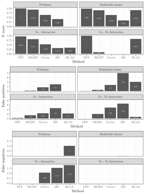
Figure 4: Barplot of results for interaction detection. The top row gives the average $F_{1}$ score for each method for detecting interactions. The second row gives the average number of false positive interactions detected. The bottom row gives the average number of false negatives detected. The average for each method is given on each bar.

Our simulation settings are borrowed from several existing works; we do not compare our methods to these other works due to a lack of publicly available software.

1. (Radchenko and James,, 2010) We generate $X_{i}\sim\operatorname{Uniform}([0,1]^{P})$ where $P=50$, $N=300$, and $\sigma^{2}=1$. We let $f_{0}(x)$ be

   $$\sqrt{0.5}\bigg{[}\sum_{v=1}^{V}f_{v}(x)+f_{1}(x)f_{2}(x)+f_{1}(x)f_{3}(x)\bigg{]}$$

   where $f_{1}(x)=x_{1}$, $f_{2}(x)=(1+x_{2})^{-1}$, $f_{3}=\sin(x_{3})$, $f_{4}(x)=e^{x_{4}}$, and $f_{5}(x)=x_{5}^{2}$. Each $f_{v}(x)$ is further centered and scaled so that $E(f_{v}(X_{i}))=0$ and $\operatorname{Var}(f_{v}(X_{i}))=1$.

2. (Vo and Pati,, 2016) We generate $X_{i}\sim\operatorname{Normal}(\bm{0},\mathrm{I})$ with $N=100$, $P=100$, and $\sigma=0.14$. We let $f_{0}(x)=x_{1}+x_{2}^{2}+x_{3}+x_{4}^{2}+x_{5}+x_{1}x_{2}+x_{2}x_{3}+x_{3}x_{4}.$

3. Same as (S2), but without the interaction effects.

4. (Friedman,, 1991) A common test case for BART, we generate $X_{i}\sim\operatorname{Uniform}([0,1]^{P})$ with $P=250,N=250$, and $\sigma^{2}=1$. We set $f_{0}(x)=10\sin(x_{1}x_{2})+20(x_{3}-0.5)^{2}+10x_{4}+5x_{5}.$

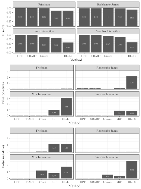
Figure 5: Barplot of results for detecting main effects.

Each of these scenarios was replicated $100$ times. We evaluate each method according to the average number of false positives (FPs), false negatives (FNs), $F_{1}$ score, and integrated root-mean squared error $\|f_{0}-\widehat{f}\|_{2}$. The $F_{1}$ score is a commonly used measure of overall accuracy that balances false positives against false negatives in variable selection tasks; see, for example, Zhang and Yang, (2015).

Results for interaction detection are given in Figure 4. We omit the results for HL because HL-LS performs uniformly better. Under all simulation settings, DP-Forests perform better than all other methods according to $F_{1}$ score. SBART is also competitive with other procedures on many of the datasets. As expected, the primary problem with SBART is that it has a relatively large number of false positives, i.e. it is susceptible to detecting spurious interactions. This issue is most pronounced on (S2) and (S3), with SBART detecting between 1.5 and 2 spurious interactions.

Additive groves and iterative random forests generally perform worse than SBART. In addition to having a larger false positives rate, these procedures are also prone to false negatives under simulation (S2). With the exception of (S1), the hierarchical group-lasso (HL-LS) performs worse than the other methods. Under (S1), HL-LS has reasonable performance as each component of $f_{0}(x)$ can be reasonably well-approximated by the assumed linear model. HL-LS also appears to perform well under (S3); this, however, is due to the fact that HL-LS typically misses several main effects, which is a substantially worse outcome than detecting a spurious interaction. The nonlinearities under (S2) and (S4) also create problems for HL-LS.

All methods perform better for detecting the main effects. SBART and DP-Forests give identical results for the main effects due to the use of SBART in screening for DP-Forests. (S1) is the easiest setting, with all methods having very few false negatives and HL-LS the only method having non-negligible false-positives. Under (S2), the non-Bayesian procedures all have non-negligible false negatives, and iRF and HL-LS are additionally prone to false positives; the story is similar under (S3), with HL-LS performing better in terms of false positives but worse in terms of false negatives. All methods perform well in terms of false positives under (S4), however iRF and HL-LS also suffer from many false negatives.

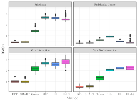
Figure 6: Boxplots given the distribution of integrated root mean-squared error for each method for each simulation setting.

Results for assessing prediction performance in terms of integrated root mean-squared error (RMSE) are given in Figure 6. SBART and DP-Forests perform very similarly in terms of RMSE. All other methods perform substantially worse under all settings. This is likely due to a multitude of factors. First, any false negatives will contribute to poor predictive performance. Second, SBART and DP-Forests are able to take advantage of underlying smoothness in the response function which additive groves and iterative random forests cannot, while HL and HL-LS suffer from an incorrect model specification.

SBART and DP-Forests are competitive in terms of runtime. For example, on a single replicate of (S4), SBART and DP-Forests took 118 seconds and 241 seconds respectively to obtain 40,000 samples from the posterior. By comparison, iRF took 279 second, HL-LS took 91 seconds, and additive groves took 4966 seconds. Additive groves was by far the slowest procedure, due to the fact that recursive feature elimination is used. We conclude that, under these settings, DP-Forests outperform all competitors are a competitive computational budget.

We also consider the publicly available Boston housing dataset of Harrison and Rubinfeld, (1978). Analysis of the interaction structures present in this dataset was previously undertaken by Radchenko and James, (2010) and Vo and Pati, (2016). This dataset consists of $P=13$ predictors and $N=506$ neighborhoods, and a continuous response corresponding to the median house value in a given neighborhood.

Method	RMSE
DP-Forests	1.00
iRF	1.22
HL	1.18
Additive Groves	1.16

Table 1: Cross-validation estimate of root mean-squared prediction error on the Boston housing dataset normalized by the RMSE of the DP-Forest.

We compare the methods in terms of goodness-of-fit, which is evaluated using a 5-fold cross validated estimate of root mean squared prediction error. Results are given in Table 1. For prediction, the DP-Forest and SBART outperform the competing methods.

The DP-Forest includes most of the predictors in the model. This can be contrasted with the fit of a sparse additive model (SPAM) Ravikumar et al., (2007) and the fit of the VANISH model reported by Radchenko and James, (2010), which include only a small number of predictors. Like the VANISH algorithm, the DP-Forest selects one interaction: there is strong evidence of an interaction between DIS (distance to an employment center in Boston) and LSTAT (the proportion of individuals in a neighborhood who are lower-status). This interaction was highly stable, and was selected by every fit to the data during cross-validation; additionally, this interaction was selected by additive groves in 4 out of 5 folds during cross-validation. Interestingly, this interaction was reportedly not selected by VANISH, which instead selects an interaction between the variables NOX (nitrus-oxide concentration) and LSTAT.

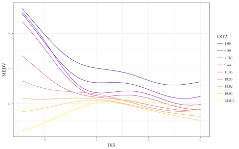
Figure 7: Graphical summary of the effect of distance DIS on MEDV for various values of LSTAT.

Figure 7 gives a visualization of the LSTAT-DIS interaction. To summarize the interaction we use a “fit-the-fit” strategy and fit a generalized additive model to the fitted-values of the DP-Forest with a thin plate spline term for the interaction (Wood,, 2003). The plot then displays the LSTAT-specific effect of DIS for the $10^{\text{th}},20^{\text{th}},\ldots,90^{\text{th}}$ quantiles of LSTAT. This GAM nearly reproduces the fitted values from the DP-Forest and is easier to visualize. We see in Figure 7 a clear interaction between DIS and LSTAT. Intuitively, one expects that the closer a neighborhood is to an industry center the more expensive the housing will be. This is correct for areas with fewer lower-status individuals; however, this trend does not hold when there is a higher percentage of lower-status individuals. We remark also that the data is well supported near $0$ for all values of LSTAT, so that this behavior is unlikely to be due to extrapolation, though extrapolation may be an issue for large values of both LSTAT and DIS.

5 DISCUSSION

We have introduced Dirichlet process forests (DP-Forests) and applied them to the problem of interaction detection. We demonstrated on both synthetic and real data that DP-Forests lead to improved interaction detection. Additionally, we demonstrated that DP-Forests are highly competitive with commonly used machine learning techniques for detecting low-order interactions.

There are a number of modifications one might make to improve performance further. One possibility is to allow $\sigma_{\mu}$ to also vary by mixture component. This would allow different mixture components to have different signal levels; for example, under simulation (S4), we would expect that a smaller value of $\sigma^{2}_{\mu}$ is appropriate for the mixture component responsible for $x_{5}$ relative to $x_{4}$. The proposed DP-Forests model captures this feature only indirectly through the number of trees assigned to each mixture component.

Additionally, it would be interesting to quantify the improvement in performance of DP-Forests over SBART theoretically. It is unknown whether SBART is variable-selection consistent, and establishing theoretically that DP-Forests are consistent for interaction detection while SBART is not remains an open problem.

References

- Basu et al., (2018) Basu, S., Kumbier, K., Brown, J. B., and Yu, B. (2018). iterative random forests to discover predictive and stable high-order interactions. Proceedings of the National Academy of Sciences, page 201711236.
- Bien et al., (2013) Bien, J., Taylor, J., and Tibshirani, R. (2013). A lasso for hierarchical interactions. Annals of statistics, 41(3):1111.
- Bleich et al., (2014) Bleich, J., Kapelner, A., George, E. I., and Jensen, S. T. (2014). Variable selection for BART: An application to gene regulation. The Annals of Applied Statistics, 8(3):1750–1781.
- Chipman et al., (2013) Chipman, H., George, E. I., Gramacy, R. B., and McCulloch, R. (2013). Bayesian treed response surface models. Wiley Interdisciplinary Reviews: Data Mining and Knowledge Discovery, 3(4):298–305.
- Chipman et al., (2010) Chipman, H. A., George, E. I., and McCulloch, R. E. (2010). BART: Bayesian additive regression trees. The Annals of Applied Statistics, 4(1):266–298.
- Ferguson, (1973) Ferguson, T. S. (1973). A Bayesian analysis of some nonparametric problems. The Annals of Statistics, 1:209–230.
- Friedman, (1991) Friedman, J. H. (1991). Multivariate adaptive regression splines. The Annals of Statistics, 19(1):1–67.
- Hahn et al., (2017) Hahn, P. R., Murray, J. S., and Carvalho, C. (2017). Bayesian regression tree models for causal inference: regularization, confounding, and heterogeneous effects. arXiv preprint arXiv:1706.09523.
- Harrison and Rubinfeld, (1978) Harrison, D. and Rubinfeld, D. L. (1978). Hedonic prices and demand for clean air. Journal of Environmental Economics and Management, 5:81–102.
- Hastie, (2017) Hastie, T. J. (2017). Generalized additive models. In Statistical models in S, pages 249–307. Routledge.
- Irsoy et al., (2012) Irsoy, O., Yildiz, O. T., and Alpaydin, E. (2012). Soft decision trees. In Proceedings of the International Conference on Pattern Recognition.
- Kapelner and Bleich, (2016) Kapelner, A. and Bleich, J. (2016). bartMachine: Machine learning with Bayesian additive regression trees. Journal of Statistical Software, 70(4):1–40.
- Lim and Hastie, (2015) Lim, M. and Hastie, T. (2015). Learning interactions via hierarchical group-lasso regularization. Journal of Computational and Graphical Statistics, 24(3):627–654.
- Linero, (2016) Linero, A. R. (2016). Bayesian regression trees for high dimensional prediction and variable selection. Journal of the American Statistical Association. To appear.
- Linero, (2017) Linero, A. R. (2017). A review of tree-based Bayesian methods. Communications for Statistical Applications and Methods, 24(6):543–559.
- Linero and Yang, (2017) Linero, A. R. and Yang, Y. (2017). Bayesian regression tree ensembles that adapt to smoothness and sparsity. arXiv preprint arXiv:1707.09461.
- Murray, (2017) Murray, J. S. (2017). Log-linear Bayesian additive regression trees for categorical and count responses. arXiv preprint arXiv:1701.01503.
- Neal, (2003) Neal, R. M. (2003). Slice sampling. The Annals of Statistics, 31:705–767.
- Pratola, (2016) Pratola, M. (2016). Efficient Metropolis-Hastings proposal mechanisms for Bayesian regression tree models. Bayesian Analysis, 11(3):885–911.
- Radchenko and James, (2010) Radchenko, P. and James, G. M. (2010). Variable selection using adaptive nonlinear interaction structures in high dimensions. Journal of the American Statistical Association, 105(492):1541–1553.
- Ravikumar et al., (2007) Ravikumar, P., Liu, H., Lafferty, J., and Wasserman, L. (2007). SPAM: Sparse additive models. In Proceedings of the 20th International Conference on Neural Information Processing Systems, pages 1201–1208.
- Rockova and van der Pas, (2017) Rockova, V. and van der Pas, S. (2017). Posterior concentration for Bayesian regression trees and their ensembles. arXiv preprint arXiv:1078.08734.
- Sorokina et al., (2008) Sorokina, D., Caruana, R., Riedewald, M., and Fink, D. (2008). Detecting statistical interactions with additive groves of trees. In Proceedings of the 25th international conference on Machine learning, pages 1000–1007. ACM.
- Sparapani et al., (2016) Sparapani, R. A., Logan, B. R., McCulloch, R. E., and Laud, P. W. (2016). Nonparametric survival analysis using Bayesian additive regression trees (BART). Statistics in medicine.
- Starling et al., (2018) Starling, J. E., Murray, J. S., Carvalho, C. M., Bukowski, R., and Scott, J. G. (2018). Functional response regression with funbart: an analysis of patient-specific stillbirth risk. arXiv preprint arXiv:1805.07656.
- Teh et al., (2006) Teh, Y. W., Jordan, M. I., Beal, M. J., and Blei, D. M. (2006). Hierarchical Dirichlet processes. Journal of the American Statistical Association, 101(476):1566–1581.
- Vo and Pati, (2016) Vo, G. and Pati, D. (2016). Sparse additive Gaussian process with soft interactions. arXiv preprint arXiv:1607.02670.
- Wang et al., (2007) Wang, H., Li, R., and Tsai, C.-L. (2007). Tuning parameter selectors for the smoothly clipped absolute deviation method. Biometrika, 94(3):553–568.
- Wood, (2003) Wood, S. N. (2003). Thin plate regression splines. Journal of the Royal Statistical Society: Series B (Statistical Methodology), 65(1):95–114.
- Zhang and Yang, (2015) Zhang, Y. and Yang, Y. (2015). Cross-validation for selecting a model selection procedure. Journal of Econometrics, 187(1):95–112.