Understanding Convolutional Neural Networks for Text Classification

Abstract

We present an analysis into the inner workings of Convolutional Neural Networks (CNNs) for processing text. CNNs used for computer vision can be interpreted by projecting filters into image space, but for discrete sequence inputs CNNs remain a mystery. We aim to understand the method by which the networks process and classify text. We examine common hypotheses to this problem: that filters, accompanied by global max-pooling, serve as ngram detectors. We show that filters may capture several different semantic classes of ngrams by using different activation patterns, and that global max-pooling induces behavior which separates important ngrams from the rest. Finally, we show practical use cases derived from our findings in the form of model interpretability (explaining a trained model by deriving a concrete identity for each filter, bridging the gap between visualization tools in vision tasks and NLP) and prediction interpretability (explaining predictions). Code implementation is available online at github.com/sayaendo/interpreting-cnn-for-text.

1 Introduction

Convolutional Neural Networks (CNNs), originally invented for computer vision, have been shown to achieve strong performance on text classification tasks Bai et al. (2018); Kalchbrenner et al. (2014); Wang et al. (2015); Zhang et al. (2015); Johnson and Zhang (2015); Iyyer et al. (2015) as well as other traditional Natural Language Processing (NLP) tasks Collobert et al. (2011), even when considering relatively simple one-layer models Kim (2014).

As with other architectures of neural networks, explaining the learned functionality of CNNs is still an active research area. The ability to interpret neural models can be used to increase trust in model predictions, analyze errors or improve the model Ribeiro et al. (2016). The problem of interpretability in machine learning can be divided into two concrete tasks: Given a trained model, model interpretability aims to supply a structured explanation which captures what the model has learned. Given a trained model and a single example, prediction interpretability aims to explain how the model arrived at its prediction. These can be further divided into white-box and black-box techniques. While recent works have begun to supply the means of interpreting predictions Alvarez-Melis and Jaakkola (2017); Lei et al. (2016); Guo et al. (2018), interpreting neural NLP models remains an under-explored area.

Accompanying their rising popularity, CNNs have seen multiple advances in interpretability when used for computer vision tasks Zeiler and Fergus (2014). These techniques unfortunately do not trivially apply to discrete sequences, as they assume a continuous input space used to represent images. Intuitions about how CNNs work on an abstract level also may not carry over from image inputs to text—for example, pooling in CNNs has been used to induce deformation invariance LeCun et al. (1998, 2015), which is likely different than the role it has when processing text.

In this work, we examine and attempt to understand how CNNs process text, and then use this information for the more practical goals of improving model-level and prediction-level explanations.

We identify and refine current intuitions as to how CNNs work. Specifically, current common wisdom suggests that CNNs classify text by working through the following steps Goldberg (2016):

1. 1-dimensional convolving filters are used as ngram detectors, each filter specializing in a closely-related family of ngrams.

2. Max-pooling over time extracts the relevant ngrams for making a decision.

3. The rest of the network classifies the text based on this information.

We refine items 1 and 2 and show that:

• Max-pooling induces a thresholding behavior, and values below a given threshold are ignored when (i.e. irrelevant to) making a prediction. Specifically, we show an experiment for which 40% of the pooled ngrams on average can be dropped with no loss of performance (Section 4).

• Filters are not homogeneous, i.e. a single filter can, and often does, detect multiple distinctly different families of ngrams (Section 5.3).

• Filters also detect negative items in ngrams—they not only select for a family of ngrams but often actively suppress a related family of negated ngrams (Section 5.4).

We also show that the filters are trained to work with naturally-occurring ngrams, and can be easily misled (made to produce values substantially larger than their expected range) by selected non-natural ngrams.

These findings can be used for improving model-level and prediction-level interpretability (Section 6). Concretely: 1) We improve model interpretability by deriving a useful summary for each filter, highlighting the kinds of structures it is sensitive to. 2) We improve prediction interpretability by focusing on informative ngrams and taking into account also the negative cues.

2 Background: 1D Text Convolutions

We focus on the task of text classification. We consider the common architecture in which each word in a document is represented as an embedding vector, a single convolutional layer with $m$ filters is applied, producing an $m$-dimensional vector for each document ngram. The vectors are combined using max-pooling followed by a ReLU activation. The result is then passed to a linear layer for the final classification.

For an $n$-words input text $w_{1},...,w_{n}$ we embed each symbol as $d$ dimensional vector, resulting in word vectors $\mathbf{w}_{1},...,\mathbf{w}_{n}\in R^{d}$. The resulting $d\times n$ matrix is then fed into a convolutional layer where we pass a sliding window over the text. For each $l$-words ngram:

$$\mathbf{u_{i}}=[\mathbf{w}_{i},...,\mathbf{w}_{i+\ell-1}]\in R^{d\times\ell}\ ;\ \ 0\leq i\leq n-\ell$$

And for each filter $\mathbf{f_{j}}\in R^{d\times\ell}$ we calculate $\langle\mathbf{u_{i}},\mathbf{f_{j}}\rangle$. The convolution results in matrix $\mathbf{F}\in R^{n\times m}$. Applying max-pooling across the ngram dimension results in $\mathbf{p}\in R^{m}$ which is fed into ReLU non-linearity. Finally, a linear fully-connected layer $\mathbf{W}\in R^{c\times m}$ produces the distribution over classification classes from which the strongest class is outputted. Formally:

$$\mathbf{u}_{i}=[\mathbf{w}_{i};...;\mathbf{w}_{i+\ell-1}]$$

$$F_{ij}=\langle\mathbf{u}_{i},\mathbf{f}_{j}\rangle$$

$$p_{j}=\operatorname*{ReLU}(\operatorname*{max}_{i}F_{ij})$$

$$\mathbf{o}=\operatorname*{softmax}(\mathbf{W}\mathbf{p})$$

In practice, we use multiple window sizes $\ell\in L$, $L\subsetneq\mathbb{N}$ by using multiple convolution layers in parallel and concatenating the resulting $\mathbf{p^{\ell}}$ vectors. We note that the methods in this work are applicable for dilated convolutions as well.

3 Datasets and Hyperparameters

For our empirical experiments and results presented in this work we use three text classification datasets for Sentiment Analysis, which involves classifying the input text (user reviews in all cases) between positive and negative. The specific datasets were chosen for their relative variety in size and domain as well as for the relative simplicity and interpretability of the binary sentiment analysis task.

The three datasets are: a) MR: sentence polarity dataset v1.0 introduced by Pang and Lee (2005), containing 10k evenly split short (sentences or snippets) movie reviews. b) Elec: electronic product reviews for sentiment classification introduced by Johnson and Zhang (2015), assembled from the Amazon review dataset McAuley and Leskovec (2013); McAuley et al. (2015), containing 200k train and 25k test evenly split reviews. c) Yelp Review Polarity: introduced by Zhang et al. (2015) from the Yelp Dataset Challenge 2015, containing 560k train and 38k test evenly split business reviews.

For word embeddings, we use the pre-trained GloVe Wikipedia 2014—Gigaword 5 embeddings Pennington et al. (2014), which we fine-tune with the model.

We use embedding dimension of 50, filter sizes of $\ell\in\{2,3,4\}$ words, and $m\in\{10,50\}$ filters. Models are implemented in PyTorch and trained with the Adam optimizer.

4 Identifying Important Features

Current common wisdom posits that filters serve as ngram detectors: each filter searches for a specific class of ngrams, which it marks by assigning them high scores. These highest-scoring detected ngrams survive the max-pooling operation. The final decision is then based on the set of ngrams in the max-pooled vector (represented by the set of corresponding filters). Intuitively, ngrams which any filter scores highly (relative to how it scores other ngrams) are ngrams which are highly relevant for the classification of the text.

In this section we refine this view by attempting to answer the questions: what information about ngrams is captured in the max-pooled vector, and how is it used for the final classification?

4.1 Informative vs. Uninformative Ngrams

Consider the pooled vector $\mathbf{p}\in R^{m}$ on which the classification is based. Each value $p_{j}=\text{ReLU}(\max_{i}\langle\mathbf{u_{i}},\mathbf{f_{j}}\rangle)$ stems from a filter-ngram interaction, and can be traced back to the ngram $\mathbf{u_{i}}=[\mathbf{w}_{i},...,\mathbf{w}_{i+\ell-1}]$ that triggered it. Denote the set of ngrams contributing to $\mathbf{p}$ as $S_{\mathbf{p}}$. Ngrams not in $S_{\mathbf{p}}$ do not influence the decision of the classifier. But what about the ngrams that are in $S_{\mathbf{p}}$? Previous attempts in prediction-based interpretation of CNNs for text highlight the ngrams in $S_{\mathbf{p}}$ and their scores as means of explaining the prediction. We take here a more refined view. Note that the final classification does not observe the ngram identities directly, but only through the scores assigned to them by the filters. Hence, the information in $\mathbf{p}$ must rely on the assigned scores.

Conceptually, we separate ngrams in $S_{\mathbf{p}}$ into two classes, deliberate and accidental.
Deliberate ngrams end up in $S_{\mathbf{p}}$ because they were scored high by their filter, likely because they are informative regarding the final decision. In contrast, accidental ngrams end up in $S_{\mathbf{p}}$ despite having a low score, because no other ngram scored higher than them. These ngrams are likely not informative for the classification decision. Can we tease apart the deliberate and accidental ngrams? We assume that there is threshold for each filter, where values above the threshold signal informative information regarding the classification, while values below the threshold are uninformative and can be ignored for the purpose of classification. We thus search for the threshold that separate the two classes. However, as we cannot measure directly which values $p_{j}$ influence the final decision, we opt instead for measuring correlation between $p_{j}$ values and the predicted label for the vector $\mathbf{p}$.

The linearity of the decision function $\mathbf{W}\mathbf{p}$ allows to measure exactly how much $p_{j}$ is weighted for the logit of label class $k$. The class which filter $\mathbf{f}_{j}$ contributes to is $c_{j}=\operatorname*{arg\,max}_{k}W_{kj}$. We refer to class $c_{j}$ as the class identity of filter $f_{j}$.

By assigning each filter a class identity $c_{j}$ and comparing it to the predicted label we arrive at a correlation label—whether the filter’s identity class matches the final decision by the network. Concretely, we run the classifier over a set of texts, resulting in pooled vectors $\mathbf{p}^{i}$ and network predictions $c^{i}$. For each filter $j$ we then consider the values $\mathbf{p}_{j}^{i}$ and whether $c^{i}=c_{j}$. For each filter, we obtain a dataset $(p_{j}^{1},c^{1}=c_{j}),...,(p_{j}^{D},c^{D}=c_{j})$, and we look for a threshold $t_{j}$ that separates $p_{j}^{i}$ for which $c^{i}=c_{j}$ from those where $c^{i}\neq c_{j}$.

$$(X,Y)_{j}=\{(p_{j}^{i},c^{i}=c_{j})\mid j<m\ \&\ i<D\}$$

In an ideal case, the set is linearly separable and we can easily separate informative from uninformative values: if $p_{j}^{i}>t_{j}$ then the classifier’s prediction agrees with the filter’s label, and otherwise they disagree. In practice, the set is not separable. We instead work with the purity of a filter-threshold combination, defined as the percentage of informative (correlative) ngrams which were scored above the threshold. Formally, given threshold dataset $(X,Y)$:

$$purity(f,t)=\\ \frac{\lvert\{(x,y)\in(X,Y)_{f}\ \mid\ x\geq t\ \&\ y=true\}\rvert}{\lvert\{(x,y)\in(X,Y)_{f}\ \mid\ x\geq t\}\rvert}$$

We heuristically set the threshold of a filter to the lowest value that achieves a sufficiently high purity (we experimentally find that a purity value of 0.75 works well).

In Figure 2b,c we show examples for threshold datasets for a model trained on the MR sentiment analysis task.

Threshold Effectiveness

We described a method for obtaining per-filter threshold values. But is the threshold assumption—that items below a given threshold do not participate in the decision—even correct? To assess the quality of threshold obtained by our proposal and validate the thresholding assumption, we discard values that do not pass the threshold for each filter and observe the performance of the model. Practically, we replace the ReLU non-linearity with a threshold function:

$$threshold(x,t)=\begin{cases}x,&\text{if }x\geq t\\ 0,&\text{otherwise}\end{cases}$$

Figure 1 presents the results on the MR dataset (we observed similar results on the Elec dataset). where the threshold is set for each filter separately, based on a shared purity value. If the thresholding assumption is correct and our way of deriving the threshold is effective, we expect to not see a drop in accuracy. Indeed, for purity value of 0.75, we observe that the model performance improves slightly when replacing the ReLU with a per-filter threshold, indicating that the thresholding model is indeed a good approximation for the feature behavior. The percentage of informative (non-accidental) values in $\mathbf{p}$ is roughly a linear function of the purity (Figure 1c). With a purity value of 0.75, we discard roughly 44% of the values in $\mathbf{p}$—and hence 44% of the ngrams in $S_{\mathbf{p}}$.

(a)

(b)

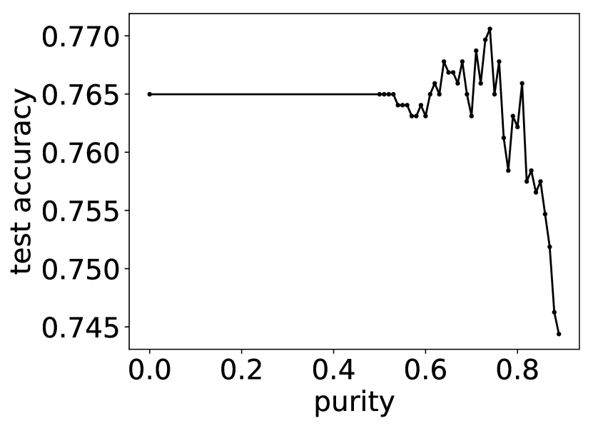
(c)

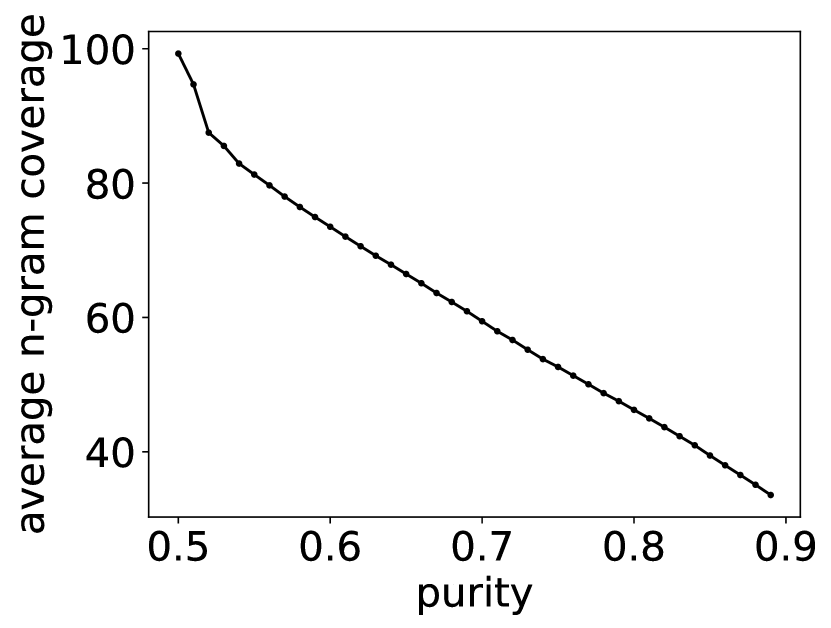
Figure 1: Evaluation results for identifying important ngrams on the MR model.

Not all filters behave in a similar way, however. In Figure 2 we show an example for a filter—#6 in the figure—which is especially uninformative: by applying the lowest threshold which satisfies a purity of 0.75, we discard 99.99% of activations. Therefore in the experiments in Figure 1, this filter is effectively unused, yet it does not cause loss in performance. In essence, the threshold classifier identified and effectively discarded a filter which is not useful to the model.

(a)

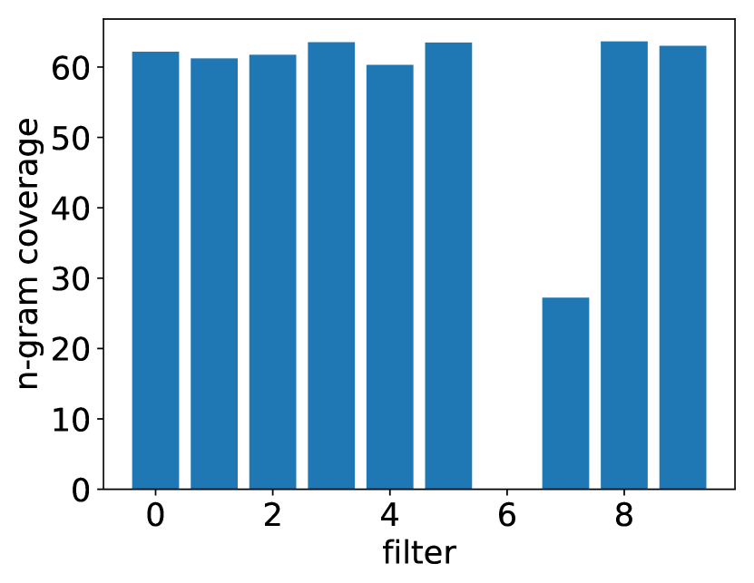
(b)

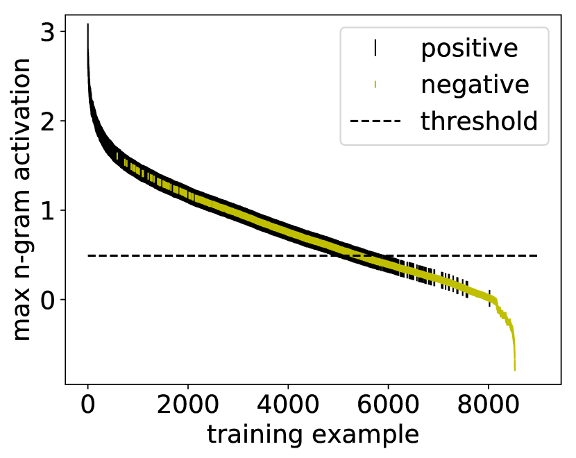
(c)

Figure 2: Visualization of informative and uninformative filters for the MR model and a universal purity of 0.75. In (a) we show the percentage of pooled ngrams which pass the threshold per filter. The threshold datasets of filters #0 and #6 are shown in (b) and (c) respectively.

To summarize,

we validated our assumptions and shown empirically that global max-pooling indeed induces a functionality of separating important and not important activation signals using a latent (presumably soft) threshold. For the rest of this work we will assume a known threshold value for every filter in the model which we can use to identify important ngrams.

5 What is captured by a filter?

Previous work looked at the top-k scoring ngrams for each filter. However, focusing on the top-k does not tell a complete story. We insead look at the set of deliberate ngrams: those that pass the filter’s threshold value. Common intuition suggests that each filter is homogeneous and specializes in detecting a specific classes of ngrams. For example, a filter may specializing in detecting ngrams such as “had no issues”, “had zero issues”, and “had no problems”. We challenge this view and show that filters often specialize in multiple distinctly different semantic classes by utilizing activation patterns which are not necessarily maximized. We also show that filters may not only identify good ngrams, but may also actively supress bad ones.

5.1 Slot Activation Vectors

As discussed in Section 2, for each ngram $\mathbf{u}=[\mathbf{w_{1}},...,\mathbf{w_{\ell}}]$ and for each filter $\mathbf{f}$ we calculate the score $\langle\mathbf{u},\mathbf{f}\rangle$. The ngram score can be decomposed as a sum of individual word scores by considering the inner products between every word embedding $\mathbf{w_{i}}$ in $\mathbf{u}$ and every parallel slice in $\mathbf{f}$:

$$\langle\mathbf{u},\mathbf{f}\rangle=\sum_{i=0}^{\ell-1}{\langle\mathbf{w_{i}},\mathbf{f_{id:i(d+1)}}\rangle}$$

We refer to slice $\mathbf{f_{id:i(d+1)}}$ as slot $i$ of the filter weights, denoted as $\mathbf{f(i)}$. Instead of taking the sum of these inner products, we can instead interpret them directly—saying that $\langle\mathbf{w_{i}},\mathbf{f(i)}\rangle$ captures how much slot $i$ in $\mathbf{f}$ is activated by the $i$th word in the ngram.

We can now move from examining the activation of an ngram-filter pair $\langle\mathbf{u}\coloneqq[\mathbf{w_{1}};...;\mathbf{w_{\ell}}],\mathbf{f}\rangle$ to examining its slot activation vector: $(\langle\mathbf{w_{1}},\mathbf{f(1)}\rangle,...,\langle\mathbf{w_{\ell}},\mathbf{f(\ell)}\rangle)$. The slot activation vector captures how much each word in the ngram contributes to its activation.

5.2 Naturally occurring vs. possible ngrams

We distinguish naturally occurring or observed ngrams, which are ngrams that are observed in a large corpus, from possible ngrams which are any combination of $\ell$ words from the vocabulary. The possible ngrams are a superset of the naturally occurring ones. Given a filter, we can find its top-scoring naturally occurring ngram by searching over all ngrams in a corpus. We can find its top-scoring possible ngram by maximizing each slot value individually. We observe there is a big and consistent gap in scores between the top-scoring natural ngrams and top-scoring possible ngrams. In our Elec model, when averaging over all filters, the top naturally-occurring ngrams score 30% less than the top possible ngrams. Interestingly, the top-scoring natural ngrams almost never fully activate all slots in a filter.

Table 1 shows the top-scoring naturally occurring and possible ngrams for nine filters in the Elec model. In each of the top scoring natural ngrams, at least one slot receives a low activation. Table 2 zooms in on one of the filters and shows its top-7 naturally occurring ngrams and top-7 most activated words in each slot. Here, most top-scoring ngrams maximize slot #3 with words such as invaluable and perfect, however some ngrams such as “works as good” and “still holding strong” maximize slots #1 and #2 respectively, instead.

Additionally, most top-scoring words do not appear to be utilized in high-scoring ngrams at all. This can be explained with the following: if a word such as crt rarely or never appears in slot #1 alongside other high-scoring words in other slots, then crt can score highly with no consequence. Since an ngram containing crt at slot #1 will rarely pass the max-pooling layer, its score at that slot is essentially random.

	top ngrams					top words by slot
filter	ngram	score	slot scores			slot #1		slot #2		slot #3		sum
0	poorly designed junk	7.31	5.47	0.97	0.87	poorly	5.47	displaying	3.06	landfill	1.75	10.28
1	simply would not	5.75	2.16	1.28	2.3	chapters	2.31	avoid	3.07	impossible	3.06	8.44
2	a minor drawback	6.11	0.88	1.85	3.38	workstation	2.06	high-quality	3.82	drawback	3.39	9.27
3	still working perfect	6.42	1.58	1.22	3.62	saves	2.52	delight	2.29	invaluable	4.19	9.0
4	absolutely gorgeous .	5.36	1.09	3.84	0.42	complain	2.57	gorgeous	3.84	expect	1.22	7.63
5	one little hitch	5.72	0.98	3.43	1.31	path	2.81	delight	4.09	everyday	2.64	9.54
6	utterly useless .	6.33	2.03	3.49	0.81	stopped	2.77	refund	3.81	disabled	1.38	7.96
7	deserves four stars	5.56	0.44	1.69	3.44	excelente	1.89	crossover	1.93	incredible	3.96	7.78
8	a mediocre product	6.91	0.35	3.11	3.45	began	1.86	mediocre	3.11	product	3.45	8.42

Table 1: Top ngrams and words by filter from a sample of nine filters from the Elec model. The average difference between the top natural ngram activation and the top possible ngram activation for this model is 2.5, or a 30% average reduction.

	top ngrams
rank	ngram	score	slot scores
1	still working perfect	6.42	1.58	1.22	3.62
2	works - perfect	5.78	1.91	0.25	3.62
3	isolation proves invaluable	5.61	0.39	1.03	4.19
4	still near perfect	5.6	1.58	0.4	3.62
5	still working great	5.45	1.58	1.22	2.65
6	works as good	5.44	1.91	1.45	2.08
7	still holding strong	5.37	1.58	1.81	1.98

top words by slot
slot #1		slot #2		slot #3
saves	2.52	delight	2.29	invaluable	4.19
crt	2.1	holding	1.81	perfect	3.62
beginner	2.09	welcome	1.8	cm	3.61
mics	2.08	dhcp	1.72	pleasant	3.38
genius	2.07	completely	1.64	simplicity	3.14
final	2.01	cradle	1.56	england	3.09
works	1.91	well-made	1.51	daily	3.04

Table 2: Top-k words by slot scores and top-k ngrams by filter scores from the Elec model. In bold are words from the top-k ngrams which appear in the top-k slot words - i.e. words which maximize their slot.

On naturally occurring ngrams, the filters do not achieve maximum values in all slots but only on some of them. Why? We consider two hypotheses to explain this behavior:

1. Each filter captures multiple semantic classes of ngrams, and each class has some dominating slots and some non-dominating slots (which we define as a slot activation pattern).

2. A slot may not be maximized because it’s not used to detect word existence, but rather lack of existence—ensuring that specific words do not occur.

We investigate both hypotheses in Sections 5.3 and 5.4 respectively.

Adversarial potential

We note in passing that this discrepancy in scores between naturally occurring and possible ngrams can be used to derive adversarial examples that cause a trained model to misclassify. By inserting a few seemingly random ngrams, we can cause filters to activate beyond their expected range, potentially driving the model to misclassification. We reserve this area of exploration for future work.

5.3 Clustering (Hypothesis (i))

We explore hypothesis (i) by clustering threshold-passing (naturally occurring) ngrams in each filter according to their activation vectors. We use Mean Shift Clustering Fukunaga and Hostetler (1975); Cheng (1995), an algorithm that does not require specifying an a-priori number of clusters, and does not make assumptions about their shapes. Mean Shift considers the feature vectors as sampled from an underlying probability density function. Each cluster captures a different slot activation pattern. We use the cluster’s centroid as the prototypical slot activation for that cluster.

Table 3 shows a sample clustering output. The clustering algorithm identified two clusters: one primarily containing ngrams of the pattern DET INTENSITY-ADVERB POSITIVE-WORD, while the second contains ngrams that begin with phrases like go wrong.

The centroids for these clusters capture the activation patterns well: low-medium-high and high-high-low for clusters 1 and 2 respectively.

ngram	slot #1	slot #2	slot #3	cluster
centroid	0.75	1.97	2.79	1
was super intriguing	1.01	3.16	5.84	1
am so grateful	2.59	3.27	4.07	1
overall very worth	3.84	1.86	4.22	1
also well worth	1.83	3.06	4.22	1
- super compassionate	0.51	3.17	5.01	1
a well oiled	0.75	3.06	4.84	1
centroid	2.87	2.17	0.12	2
go wrong bringing	3.97	4.12	1.81	2
go wrong pairing	3.97	4.12	1.65	2
go wrong when	3.97	4.12	-0.4	2

Table 3: Example clustering results on the Yelp dataset. After applying thresholds, the ngrams for this filter were split into two clusters of sizes 83% and 17% respectively. The table shows top-scoring ngrams for this filter with their clustering results, sorted by their activation strength.

To summarize,

by discarding noisy ngrams which do not pass the filter’s threshold and then clustering those that remain according to their slot activation patterns, we arrived at a clearer image of the semantic classes of ngrams that a given filter specializes in capturing. In particular, we reveal that filters are not necessarily homogeneous: a single filter may detect several different semantic patterns, each one of them relying on a different slot activation pattern.

5.4 Negative Ngrams (Hypothesis (ii))

Our second theory to explain the discrepancy between the activations of naturally occurring and possible ngrams is that certain filter slots are not used to detect a class of highly activating words, but rather to rule out a class of highly negative words. We refer to these as negative ngrams.

For example, Table 3 shows an ngram pattern for which slot #1 contains determiners and other “filler” tokens such as hyphens, periods and commas with relatively weak slot activations. Hypothesis (ii) suggests that this slot may receive a strong negative score for words such as not and n’t, causing such negated patterns to drop below the threshold. Indeed, ngrams containing not or n’t in slot #1 do not pass the threshold for this filter.

We are interested in a more systematic method of identifying these cases. Identifying negative slot activations would be very useful for understanding the semantics captured by a filter and the reasoning behind the dismissal of an ngram, as we discuss in Sections 6.1 and 6.2 respectively.

We achieve this by searching the below-threshold ngram space for ngrams which are “flipped versions” of above-threshold ngrams. Concretely: Given ngram $\mathbf{u}$ which was scored highly by filter $\mathbf{f}$, we search for low-scoring ngrams $\mathbf{u^{\prime}}$ such that the hamming distance between $\mathbf{u}$ and $\mathbf{u^{\prime}}$ is low. By doing this for the top-k scoring ngrams per cluster, we arrive at a comprehensive set of negative ngrams. In Table 4 we show a sample output of this algorithm.

Furthermore, we can divide negative ngrams into two cases: 1) Lowering the ngram score below the threshold by replacing high-scoring words with low-scoring words. 2) Lowering the ngram score below the threshold by replacing words with a low positive score with words with a highly-negative score. Case 2 is more interesting because it embodies cases where hypothesis (ii) is relevant. Additionally, it highlights ngrams where a strongly positive word in one slot was negated with another strongly negative word in another slot. Table 4 shows examples in bold.

In order to identify “Case 2” negative ngrams, we heuristically test whether the “changed” words’ scores directly influence the status of the activation relative to the threshold: given an already identified negative ngram, if the ngram score—sans the bottom-k negative slot activations (considering a hamming distance of $k$ and given that there are $k$ negative slot activations)—passes the threshold, yet it does not pass the threshold by including the negative slot activations, then the ngram is considered a “Case 2” negative ngram.

ngram	slot #1	slot #2	slot #3	sum
’m really pleased	2.59	1.86	5.05	9.5
’m really not			-2.49	1.96
’m really upset			-1.14	3.31
’m not pleased		-3.4		4.24
is extremely useful	2.3	3.24	3.96	9.5
is extremely limited			-2.8	2.74
is extremely noisy			-2.77	2.8
is not useful		-3.4		2.86
is only useful		-2.82		3.44
is surprisingly good	2.3	4.32	2.8	9.42
is not good		-3.4		1.7
is only good		-2.82		2.28
is no good		-1.88		3.22
is probably good		-1.66		3.44
am very satisfied	2.01	2.17	5.09	9.26
am very dissatisfied			-1.9	2.27
am very disappointed			-1.87	2.3
am not satisfied		-3.4		3.69
not very satisfied	-2.6			4.66

Table 4: Top-scoring ngrams from one filter from a model trained on the Elec dataset, and their accompanying lowest-scoring negative ngrams. We selected a hamming distance of 1 word. Bold ngrams are Case 2 negative ngrams.

6 Interpretability

In this section we show two practical implications of the findings above: improvements in both model-level and prediction-level interpretability of 1D CNNs for text classification.

6.1 Model Interpretability

As in computer vision, we can now interpret a trained CNN model by “visualizing” its filters and interpreting the visible shapes—in other words, defining a high-level description of what the filter detects. We propose to associate each filter with the following items: 1) The class which this filter’s strong signals contribute to (in the sentiment task: positive or negative); 2) The threshold value for the filter, together with its purity and coverages percentages (which essentially capture how informative this filter is); 3) A list of semantic patterns identified by this filter. Each list item corresponds to a slot-activations cluster. For each cluster we present the top-k ngrams activating it, and for each ngram we specify its total activation, its slot-activation vector, and its list of bottom-k negative ngrams with their activations and slot activations. In particular, by clustering the activated ngrams according to their slot activation patterns and showing the top-k in each clusters, we get a much more refined coverage of the linguistic patterns that are captured by the filter.

6.2 Prediction Interpretability

Previous prediction-based interpretation attempts traced back the ngrams from the max-pooling layer. Here we improve these previous attempts by considering only ngrams that pass the threshold for their filter. This results in a more concise and relevant explanation (Figure 1). Figure 3 shows two examples. Note that in example #1, many negative-class filters were “forced” to choose an ngram in max-pooling despite there not being strongly negative phrases—but those ngrams do not pass the threshold and are thus cleaned from the explanation.

Additionally we can use the individual slot activations to tease-apart the contribution of each word in the ngram. Finally, we can also mark cases of negative-ngrams (Section 5.4), where an ngram has high slot activations for some words, but these are negated by a highly-negative slot and as a consequence are not selected by max-pooling, or are selected but do not pass the filter’s threshold.

my UNK fits perfectly . very well made . nice looking and offers good protection
filter	f-class	ngram	slot scores
0	pos	PAD PAD my	0.7	1.65	0.16
1	pos	. very well	0.98	2.17	2.63
2	neg	PAD my UNK	1.31	-0.07	0.21
3	neg	UNK fits perfectly	0.28	0.61	0.03
4	neg	looking and offers	0.6	0.12	0.5
5	neg	good protection PAD	0.52	1.6	-0.01
6	pos	UNK fits perfectly	-0.06	2.36	1.82
7	neg	fits perfectly .	1.34	-0.71	1.47
8	neg	. very well	-0.01	1.97	-0.55
9	pos	perfectly . very	4.13	0.45	-0.01
this product sucked was not loud at all lights did n’t work overall a bad product that ’s UNK taking up space
filter	f-class	ngram	slot scores
0	pos	product sucked was	0.12	2.05	0.1
1	pos	overall a bad	2.53	1.4	-1.16
2	neg	lights did n’t	-0.33	1.12	1.63
3	neg	PAD this product	-0.2	1.43	0.51
4	neg	did n’t work	1.21	0.97	2.65
5	neg	sucked was not	0.98	0.59	1.32
6	pos	work overall a	-0.25	4.05	-0.21
7	neg	was not loud	-0.33	2.85	0.52
8	neg	a bad product	-0.45	3.08	1.32
9	pos	PAD PAD this	0.38	0.15	1.66

Figure 3: Examples predicted positive and negative respectively by a model trained on the Elec dataset, along with their explanations. Ngrams which passed the threshold are in bold, and case 2 negative ngrams are in italics. For clarity’s sake we trained a small model which uses ten filters.

7 Conclusion

We have refined several common wisdom assumptions regarding the way in which CNNs process and classify text. First, we have shown that max-pooling over time induces a thresholding behavior on the convolution layer’s output, essentially separating between features that are relevant to the final classification and features that are not. We used this information to identify which ngrams are important to the classification. We also associate each filter with the class it contributes to. We decompose the ngram score into word-level scores by treating the convolution of a filter as a sum of word-level convolutions, allowing us to examine the word-level composition of the activation. Specifically, by maximizing the word-level activations by iterating over the vocabulary, we observed that filters do not maximize activations at the word-level, but instead form slot activation patterns that give different types of ngrams similar activation strengths. This provides empirical evidence that filters are not homogeneous. By clustering high-scoring ngrams according to their slot-activation patterns we can identify the groups of linguistic patterns captured by a filter. We also show that filters sometimes opt to assign negative values to certain word activations in order to cause the ngrams which contain them to receive a low score despite having otherwise highly activating words. Finally, we use these findings to suggest improvements to model-based and prediction-based interpretability of CNNs for text.

References

- Alvarez-Melis and Jaakkola (2017) David Alvarez-Melis and Tommi S. Jaakkola. 2017. A causal framework for explaining the predictions of black-box sequence-to-sequence models. In Proceedings of the 2017 Conference on Empirical Methods in Natural Language Processing, EMNLP 2017, Copenhagen, Denmark, September 9-11, 2017, pages 412–421. Association for Computational Linguistics.
- Bai et al. (2018) Shaojie Bai, J. Zico Kolter, and Vladlen Koltun. 2018. An empirical evaluation of generic convolutional and recurrent networks for sequence modeling. CoRR, abs/1803.01271.
- Cheng (1995) Yizong Cheng. 1995. Mean shift, mode seeking, and clustering. IEEE Trans. Pattern Anal. Mach. Intell., 17(8):790–799.
- Collobert et al. (2011) Ronan Collobert, Jason Weston, Léon Bottou, Michael Karlen, Koray Kavukcuoglu, and Pavel P. Kuksa. 2011. Natural language processing (almost) from scratch. Journal of Machine Learning Research, 12:2493–2537.
- Fukunaga and Hostetler (1975) Keinosuke Fukunaga and Larry D. Hostetler. 1975. The estimation of the gradient of a density function, with applications in pattern recognition. IEEE Trans. Information Theory, 21(1):32–40.
- Goldberg (2016) Yoav Goldberg. 2016. A primer on neural network models for natural language processing. J. Artif. Intell. Res., 57:345–420.
- Guo et al. (2018) Pei Guo, Connor Anderson, Kolten Pearson, and Ryan Farrell. 2018. Neural network interpretation via fine grained textual summarization. CoRR, abs/1805.08969.
- Iyyer et al. (2015) Mohit Iyyer, Varun Manjunatha, Jordan L. Boyd-Graber, and Hal Daumé III. 2015. Deep unordered composition rivals syntactic methods for text classification. In Proceedings of the 53rd Annual Meeting of the Association for Computational Linguistics and the 7th International Joint Conference on Natural Language Processing of the Asian Federation of Natural Language Processing, ACL 2015, July 26-31, 2015, Beijing, China, Volume 1: Long Papers, pages 1681–1691. The Association for Computer Linguistics.
- Johnson and Zhang (2015) Rie Johnson and Tong Zhang. 2015. Effective use of word order for text categorization with convolutional neural networks. In NAACL HLT 2015, The 2015 Conference of the North American Chapter of the Association for Computational Linguistics: Human Language Technologies, Denver, Colorado, USA, May 31 - June 5, 2015, pages 103–112. The Association for Computational Linguistics.
- Kalchbrenner et al. (2014) Nal Kalchbrenner, Edward Grefenstette, and Phil Blunsom. 2014. A convolutional neural network for modelling sentences. In Proceedings of the 52nd Annual Meeting of the Association for Computational Linguistics, ACL 2014, June 22-27, 2014, Baltimore, MD, USA, Volume 1: Long Papers, pages 655–665. The Association for Computer Linguistics.
- Kim (2014) Yoon Kim. 2014. Convolutional neural networks for sentence classification. In Proceedings of the 2014 Conference on Empirical Methods in Natural Language Processing, EMNLP 2014, October 25-29, 2014, Doha, Qatar, A meeting of SIGDAT, a Special Interest Group of the ACL, pages 1746–1751. ACL.
- LeCun et al. (2015) Yann LeCun, Y Bengio, and Geoffrey Hinton. 2015. Deep learning. 521:436–44.
- LeCun et al. (1998) Yann LeCun, Leon Bottou, Y Bengio, and Patrick Haffner. 1998. Gradient-based learning applied to document recognition. 86:2278 – 2324.
- Lei et al. (2016) Tao Lei, Regina Barzilay, and Tommi S. Jaakkola. 2016. Rationalizing neural predictions. In Proceedings of the 2016 Conference on Empirical Methods in Natural Language Processing, EMNLP 2016, Austin, Texas, USA, November 1-4, 2016, pages 107–117. The Association for Computational Linguistics.
- McAuley and Leskovec (2013) Julian J. McAuley and Jure Leskovec. 2013. Hidden factors and hidden topics: understanding rating dimensions with review text. In Seventh ACM Conference on Recommender Systems, RecSys ’13, Hong Kong, China, October 12-16, 2013, pages 165–172. ACM.
- McAuley et al. (2015) Julian J. McAuley, Christopher Targett, Qinfeng Shi, and Anton van den Hengel. 2015. Image-based recommendations on styles and substitutes. In Proceedings of the 38th International ACM SIGIR Conference on Research and Development in Information Retrieval, Santiago, Chile, August 9-13, 2015, pages 43–52. ACM.
- Pang and Lee (2005) Bo Pang and Lillian Lee. 2005. Seeing stars: Exploiting class relationships for sentiment categorization with respect to rating scales. CoRR, abs/cs/0506075.
- Pennington et al. (2014) Jeffrey Pennington, Richard Socher, and Christopher D. Manning. 2014. Glove: Global vectors for word representation. In Empirical Methods in Natural Language Processing (EMNLP), pages 1532–1543.
- Ribeiro et al. (2016) Marco Túlio Ribeiro, Sameer Singh, and Carlos Guestrin. 2016. ”why should I trust you?”: Explaining the predictions of any classifier. In Proceedings of the 22nd ACM SIGKDD International Conference on Knowledge Discovery and Data Mining, San Francisco, CA, USA, August 13-17, 2016, pages 1135–1144. ACM.
- Ruderman et al. (2018) Avraham Ruderman, Neil C. Rabinowitz, Ari S. Morcos, and Daniel Zoran. 2018. Learned deformation stability in convolutional neural networks. CoRR, abs/1804.04438.
- Wang et al. (2015) Peng Wang, Jiaming Xu, Bo Xu, Cheng-Lin Liu, Heng Zhang, Fangyuan Wang, and Hongwei Hao. 2015. Semantic clustering and convolutional neural network for short text categorization. In Proceedings of the 53rd Annual Meeting of the Association for Computational Linguistics and the 7th International Joint Conference on Natural Language Processing of the Asian Federation of Natural Language Processing, ACL 2015, July 26-31, 2015, Beijing, China, Volume 2: Short Papers, pages 352–357. The Association for Computer Linguistics.
- Zeiler and Fergus (2014) Matthew D. Zeiler and Rob Fergus. 2014. Visualizing and understanding convolutional networks. In Computer Vision - ECCV 2014 - 13th European Conference, Zurich, Switzerland, September 6-12, 2014, Proceedings, Part I, volume 8689 of Lecture Notes in Computer Science, pages 818–833. Springer.
- Zhang et al. (2015) Xiang Zhang, Junbo Jake Zhao, and Yann LeCun. 2015. Character-level convolutional networks for text classification. In Advances in Neural Information Processing Systems 28: Annual Conference on Neural Information Processing Systems 2015, December 7-12, 2015, Montreal, Quebec, Canada, pages 649–657.