Systematic investigation of X-ray spectral variability of TeV blazars during flares in the RXTE era

Abstract

Utilizing all the 16-year RXTE observations, we analyze the X-ray spectra of 32 TeV blazars, and perform a systematic investigation of X-ray spectral variability for the 5 brightest sources during their major flares that lasted several days. We obtain photon spectral index ($\alpha$), flux and synchrotron radiation peak energy ($E_{\rm{p}}$) from empirical spectral fitting, and electron spectral index ($p$) from theoretical synchrotron radiation modeling. We find that both $\alpha$ and $p$ generally display a harder-when-brighter trend, confirming the results of many previous works. Furthermore, we confirm and strengthen the result that $p$ must vary in order to explain the observed X-ray spectral variability during flares, which would have useful implications for interpreting the associated higher-energy spectral variability. We see apparent electron spectral hysteresis in many but not all $p$-flux plots that takes a form of “loop” or oblique “8”. We obtain a tight $p$-hardness ratio (HR) relation and a tighter $p$-$\alpha$ relation using spectra of flaring periods, both of which are also applicable to stacked data of quiescent periods. We demonstrate that these two empirical relations can be used efficiently to estimate $p$ from HR or $\alpha$ that is readily achieved. Finally, we find that, when considering TeV blazars as a whole, $\alpha$ and X-ray luminosity are positively correlated, $E_{\rm{p}}$ is negatively correlated with $p$ and $\alpha$, and $E_{\rm{p}}$ is positively correlated with HR; all these correlations are in line with the blazar sequence. However, after correcting for the Doppler boosting effect, $\alpha$ and intrinsic X-ray luminosity follow an anti-correlation.

1 Introduction

Blazars, including Flat Spectrum Radio Quasars (FSRQs) and BL Lac objects, are a subclass of active galactic nuclei (AGNs), with one of their relativistic jets pointing to the observers at small angles (Urry & Padovani, 1995). They are the most important contributor to the cosmic TeV background radiation among extragalactic sources (e.g., Holder, 2014; Sushch & H. E. S. S. Collaboration, 2015; Inoue & Tanaka, 2016). Their jet emission presents double-hump broadband spectral energy distributions (SEDs) and intense variability in multiple wavelengths across different timescales. The low-energy peak is located between infrared and X-ray energies, and the high-energy peak is located at hard X-ray up to TeV $\gamma$-ray emission (e.g., Abdo et al., 2010a). The first hump is widely believed to be produced by the synchrotron radiation of relativistic electrons and/or positrons in the jet, while the origin of the second hump is still in dispute. In leptonic scenarios, the high-energy hump is dominated by the inverse Compton radiation derived from relativistic electrons scattering synchrotron photons (e.g., Maraschi et al., 1992; Kirk et al., 1998) and/or external photons, e.g., from the accretion disk, broad-line region or cosmic microwave background (e.g., Dermer et al., 1992; Sikora et al., 1994). In hadronic scenarios, the high-energy radiation is due to the proton emission processes (e.g., Aharonian, 2000; Mücke & Protheroe, 2001; Atoyan & Dermer, 2003; Mücke et al., 2003; Böttcher et al., 2013; Fraija & Marinelli, 2015).

According to the peak frequency of the low-energy hump ($\nu_{\textrm{p}}$), BL Lac objects can be divided into high-energy peaked BL Lac objects (HBLs), intermediate-energy peaked BL Lac objects (IBLs) and low-energy peaked BL Lac objects (LBLs; e.g., Padovani & Giommi, 1995; Fossati et al., 1998; Abdo et al., 2010a; Fan et al., 2016). For HBLs, the synchrotron peak is located in the UV to X-ray domain ($\nu_{\textrm{p}}>10^{15}\ \textrm{Hz}$); for IBLs, the peak is between optical and UV regimes ($10^{14}<\nu_{\textrm{p}}\leq 10^{15}\ \textrm{Hz}$); for LBLs, the peak is in the infrared band ($\nu_{\textrm{p}}\leq 10^{14}\ \textrm{Hz}$; Abdo et al., 2010a). Another type of blazars, FSRQs, are the high-luminosity sources whose synchrotron peak is located in the broad regime from the far-infrared to optical and even to UV wavelengths, and whose X-ray emission is from inverse Compton radiation process. As one type of sources detected at TeV energies, TeV blazars mainly belong to HBLs whose X-ray spectrum is usually dominated by synchrotron emission, therefore we use the synchrotron emission model to fit X-ray spectra of TeV blazars in this work.

The intense variability of blazars has been illustrated by, e.g., their multiple discrete X-ray flares at timescales from several months to days to minutes (e.g., Cui, 2004; Xue & Cui, 2005), with some extremely rapid flares even having characteristic rising timescales down to half a minute (Zhu et al., 2018). The flaring activities are often thought to be associated with several physical processes, such as the internal shocks generated in the jet (Rees, 1978; Spada et al., 2001), the magnetic reconnection processes in the jet (Lyutikov, 2003; Giannios et al., 2009), or the ejection events of relativistic particles into the jet (Boettcher et al., 1997; Mastichiadis & Kirk, 1997). Furthermore, many studies have revealed a harder-when-brighter trend in X-ray flares of blazars, which manifests itself in hardening of spectra with increasing fluxes (e.g., Giommi et al., 1990; Sambruna et al., 1994; Xue et al., 2006; Abdo et al., 2010b). Xue et al. (2006) used the synchrotron model to investigate the X-ray spectral variability of Mkr 421 and Mrk 501 during flares that lasted for several days. Among the four key parameters (particle spectral index, maximum Lorentz factor, total energy density and magnetic field), they found that the electron spectral index ($p$) must vary during the flaring period and it tends to decrease with increasing flux. Therefore, studying the evolution of physical parameters during flares could help us understand the underlying physical mechanism in the flaring process.

In this paper, we make use of all the 16-year archival data of TeV blazars from Proportional Counter Array (PCA) onboard Rossi X-Ray Timing Explorer (RXTE), a synchrotron radiation model, and the Markov chain Monte Carlo (MCMC) method to carry out a systematic investigation of the 3–25 keV X-ray spectral variability during flares of Mrk 421, Mrk 501, PKS 2155–304, PKS 2005–489, and 1ES 1959+650. This work builds on and extends further the work of Xue et al. (2006), and some significant improvements over Xue et al. (2006) are: our target sources for detailed analysis increase from two (i.e., Mrk 421 and Mrk 501) to five; the search of target flares covers all the RXTE/PCA observations throughout its entire lifespan ($\sim$16 years); we utilize a new method that greatly improves calculation efficiency. One primary goal of this paper is to test the universality of the conclusion in Xue et al. (2006) that multiple parameters (that characterize the electron distribution and magnetic field), in particular, the electron spectral index, must vary, in order to account for the observed X-ray spectral variability of TeV blazars during flares that lasted for days to weeks. One thing worth noting is that we only focus on the evolution of electron spectral index in this paper, as the other parameters are generally constrained poorly (see the detailed discussion in Xue et al., 2006).

Table 1: Summary of 32 TeV blazars observed by RXTE/PCA

Object	Type	Redshift(z)	$\textit{N}_{\textrm{H,Gal}}^{\textrm{(DL)}}$	$\textit{N}_{\textrm{spectra}}$	$\chi^{\textrm{2}}_{\nu\textrm{,95\%}}$(CPL)	$\textit{F}_{\textrm{max,3--25 keV}}$(CPL)	$\chi^{\textrm{2}}_{\nu\textrm{,95\%}}$(LP)	$\textit{F}_{\textrm{max,3--25 keV}}$(LP)
			$\textrm{[10}^{\textrm{20}}\ \textrm{cm}^{\textrm{--2}}\textrm{]}$			$\textrm{[}\textrm{10}^{\textrm{--12}}\ \textrm{erg}\ \textrm{cm}^{\textrm{--2}}\ \textrm{s}^{\textrm{--1}}\textrm{]}$		$\textrm{[}\textrm{10}^{\textrm{--12}}\ \textrm{erg}\ \textrm{cm}^{\textrm{--2}}\ \textrm{s}^{\textrm{--1}}\textrm{]}$
(1)	(2)	(3)	(4)	(5)	(6)	(7)	(8)	(9)
AP Librae	LBL	0.049	8.76	4	0.7035	8.18	0.7027	9.20
3C 66A	IBL	$\cdots$	8.99	99	0.8183	12.48	0.8198	13.41
BL Lacertae	IBL	0.069	21.3	1382	0.7649	68.04	0.7559	68.38
MAGIC J2001+435	IBL	$\cdots$	47.4	23	0.8488	4.96	0.8488	5.23
S5 0716+714	IBL	0.310	3.81	230	0.7965	19.67	0.7865	19.06
W Coma	IBL	0.102	1.88	13	0.7827	3.16	0.7826	4.10
1ES 0229+200	HBL	0.140	9.21	205	0.7519	56.27	0.7469	57.33
1ES 0414+009	HBL	0.287	10.3	13	0.7377	23.41	0.7233	23.63
1ES 0647+250	HBL	0.450	12.8	20	0.7475	34.11	0.7484	35.08
1ES 0806+524	HBL	0.138	4.43	20	0.7226	7.37	0.7262	7.71
1ES 1101–232	HBL	0.186	5.76	99	0.7709	57.13	0.7722	59.88
1ES 1215+303	HBL	0.130	1.69	2	0.8500	24.93	0.8439	25.25
1ES 1218+304	HBL	0.182	1.73	23	0.7640	187.23	0.7623	191.27
1ES 1727+502	HBL	0.055	2.75	17	0.6961	29.58	0.7214	30.00
1ES 1741+196	HBL	0.084	6.86	12	0.8649	27.92	0.8546	29.37
1ES 1959+650★	HBL	0.048	10.1	146	0.8966	854.55	0.8558	862.13
1ES 2344+514	HBL	0.044	16.3	53	0.8733	157.59	0.8724	160.70
H 1426+428	HBL	0.129	1.38	165	0.7850	102.78	0.7781	104.46
H 2356–309	HBL	0.165	1.33	2	0.5959	8.08	0.5988	8.74
Markarian 180	HBL	0.045	1.42	13	0.6644	17.74	0.6636	18.55
Markarian 421★	HBL	0.031	1.38	1195	0.9335	3208.60	0.9010	3209.60
Markarian 501★	HBL	0.034	1.71	495	0.8771	1003.30	0.8747	1003.80
PG 1553+113	HBL	0.500	3.67	48	0.7529	28.57	0.7461	29.87
PKS 0447–439	HBL	0.343	1.78	11	0.8627	15.88	0.8657	17.70
PKS 0548–322	HBL	0.069	2.19	5	0.5474	40.76	0.5438	42.25
PKS 1424+240	HBL	$\cdots$	2.64	64	0.8207	3.38	0.8209	3.45
PKS 2005–489★	HBL	0.071	5.08	161	0.8221	332.77	0.8150	333.69
PKS 2155–304★	HBL	0.116	1.69	502	0.8111	207.60	0.8110	213.76
RGB J0152+017	HBL	0.080	2.86	22	0.6224	9.02	0.6482	9.61
RGB J0710+591	HBL	0.125	5.60	10	0.7979	64.71	0.7942	65.88
3C 279	FSRQ	0.536	2.21	1979	0.7548	75.37	0.7483	75.85
PKS 1510–089	FSRQ	0.361	7.96	1314	0.7526	45.80	0.7382	48.54

2 DATA AND DATA REDUCTION

RXTE, carrying All Sky Monitor (ASM), PCA, and High-Energy X-Ray Timing Experiment (HEXTE), started operation in 1996 January and completed its scientific mission in 2012 January. During its 16-year lifespan, RXTE had observed 52 blazars (Rivers et al., 2013), including 32 TeV blazars (see Table 1) verified in the catalog of TeV sources (i.e., TeVCat). These TeV blazars are 2 FSRQs, 1 LBLs, 5 IBLs, and 24 HBLs.

Table 2: Spectral fitting results of 5 TeV blazars during flaring periods and quiescent periods

			Cut-off Power Law			Log-parabolic					Synchrotron
Object	Date	MJD	$\Gamma$	$\textit{F}_{\textrm{3--25 keV}}$	$\chi^{2}_{\nu}$ ($\nu$)	a	b	K	$\textit{F}_{\textrm{3--25 keV}}$	$\chi^{2}_{\nu}$ ($\nu$)	$p$	$\chi^{2}_{\nu}$ ($\nu$)
(1)	(2)	(3)	(4)	(5)	(6)	(7)	(8)	(9)	(10)	(11)	(12)	(13)
Mrk 421	$\blacktriangle$ 2001/03/20	51988.44	2.45 (0.04)	4.52	0.34 (26)	2.22 (0.10)	0.28 (0.06)	0.36 (0.03)	4.53	0.22 (26)	$\textrm{4.08}^{+\textrm{0.05}}_{-\textrm{0.07}}$	0.42 (24)
	$\blacktriangle$ 2001/03/20	51988.73	2.23 (0.04)	7.49	0.53 (32)	1.97 (0.08)	0.29 (0.05)	0.37 (0.03)	7.50	0.33 (32)	$\textrm{3.58}^{+\textrm{0.07}}_{-\textrm{0.04}}$	0.63 (30)
(flaring)	$\blacktriangle$ 2001/03/21	51989.69	2.16 (0.02)	15.47	0.66 (41)	1.80 (0.06)	0.38 (0.03)	0.65 (0.04)	15.47	0.29 (41)	$\textrm{3.45}^{+\textrm{0.05}}_{-\textrm{0.03}}$	0.80 (40)
	$\blacktriangle$ 2001/03/22	51990.04	2.26 (0.03)	7.58	0.38 (31)	1.97 (0.08)	0.33 (0.05)	0.41 (0.03)	7.60	0.22 (31)	$\textrm{3.64}^{+\textrm{0.06}}_{-\textrm{0.05}}$	0.54 (28)
	$\blacktriangle$ 2001/03/22	51990.16	2.17 (0.07)	5.65	0.57 (27)	1.77 (0.15)	0.51 (0.09)	0.28 (0.04)	5.68	0.56 (27)	$\textrm{3.58}^{+\textrm{0.12}}_{-\textrm{0.13}}$	0.58 (21)
(quiescent)	$\blacktriangledown\ \ \ \textrm{2003}^{\textrm{/04/02}}_{\textrm{/05/02}}$	$\textrm{52700}^{\textrm{+31}}_{\textrm{+63}}$	2.51 (0.06)	1.14	0.40 (22)	2.23 (0.11)	0.35 (0.07)	0.10 (0.01)	1.14	0.37 (22)	$\textrm{4.25}^{+\textrm{0.08}}_{-\textrm{0.08}}$	0.45 (21)
(quiescent)	$\blacktriangledown\ \ \ \textrm{2010}^{\textrm{/04/09}}_{\textrm{/04/18}}$	$\textrm{55000}^{\textrm{+295}}_{\textrm{+304}}$	2.48 (0.10)	0.85	0.56 (17)	2.11 (0.20)	0.49 (0.13)	0.08 (0.01)	0.85	0.47 (17)	$\textrm{4.26}^{+\textrm{0.16}}_{-\textrm{0.16}}$	0.64 (16)
Mrk 501	$\blacktriangle$ 1997/04/12	50550.19	1.72 (0.05)	5.25	0.78 (28)	1.61 (0.10)	0.12 (0.06)	0.09 (0.01)	5.25	0.67 (28)	$\textrm{2.43}^{+\textrm{0.11}}_{-\textrm{0.08}}$	0.83 (29)
	$\blacktriangle$ 1997/04/12	50550.45	1.71 (0.04)	6.00	0.73 (29)	1.62 (0.10)	0.09 (0.06)	0.10 (0.01)	6.00	0.64 (29)	$\textrm{2.39}^{+\textrm{0.09}}_{-\textrm{0.08}}$	0.66 (30)
(flaring)	$\blacktriangle$ 1997/04/13	50551.46	1.59 (0.04)	7.84	0.77 (35)	1.46 (0.08)	0.15 (0.05)	0.10 (0.01)	7.84	0.65 (35)	$\textrm{2.11}^{+\textrm{0.11}}_{-\textrm{0.07}}$	0.80 (37)
	$\blacktriangle$ 1997/04/14	50552.34	1.64 (0.04)	6.20	1.14 (28)	1.52 (0.10)	0.13 (0.06)	0.09 (0.01)	6.21	1.02 (28)	$\textrm{2.28}^{+\textrm{0.07}}_{-\textrm{0.12}}$	1.18 (31)
	$\blacktriangle$ 1997/04/15	50553.27	1.69 (0.04)	6.12	0.52 (27)	1.58 (0.08)	0.11 (0.05)	0.09 (0.01)	6.12	0.49 (27)	$\textrm{2.37}^{+\textrm{0.07}}_{-\textrm{0.09}}$	0.55 (27)
(quiescent)	$\blacktriangledown\ \ \ \textrm{2004}^{\textrm{/06/14}}_{\textrm{/06/21}}$	$\textrm{53100}^{\textrm{+70}}_{\textrm{+77}}$	2.07 (0.07)	1.06	0.65 (20)	1.82 (0.13)	0.30 (0.08)	0.04 (0.005)	1.06	0.58 (20)	$\textrm{3.23}^{+\textrm{0.16}}_{-\textrm{0.16}}$	0.70 (19)
(quiescent)	$\blacktriangledown\ \ \ \textrm{1998}^{\textrm{/06/19}}_{\textrm{/06/23}}$	$\textrm{50980}^{\textrm{+2}}_{\textrm{+7}}$	2.11 (0.06)	0.71	0.40 (22)	2.04 (0.12)	0.08 (0.07)	0.03 (0.003)	0.72	0.40 (22)	$\textrm{3.26}^{+\textrm{0.07}}_{-\textrm{0.10}}$	0.42 (21)
PKS 2155–304	$\blacktriangle$ 1996/05/19	50222.65	2.32 (0.07)	1.10	0.47 (25)	2.16 (0.15)	0.22 (0.10)	0.07 (0.01)	1.10	0.43 (25)	$\textrm{3.78}^{+\textrm{0.09}}_{-\textrm{0.11}}$	0.45 (22)
	$\blacktriangle$ 1996/05/19	50222.80	2.28 (0.07)	1.36	0.35 (26)	2.15 (0.14)	0.17 (0.09)	0.08 (0.01)	1.37	0.35 (26)	$\textrm{3.65}^{+\textrm{0.09}}_{-\textrm{0.09}}$	0.37 (23)
(flaring)	$\blacktriangle$ 1996/05/20	50223.55	2.25 (0.06)	1.84	0.56 (28)	2.05 (0.14)	0.26 (0.09)	0.10 (0.01)	1.85	0.50 (28)	$\textrm{3.62}^{+\textrm{0.11}}_{-\textrm{0.09}}$	0.61 (25)
	$\blacktriangle$ 1996/05/21	50223.93	2.21 (0.05)	1.71	0.22 (26)	1.99 (0.12)	0.28 (0.07)	0.09 (0.01)	1.72	0.23 (26)	$\textrm{3.54}^{+\textrm{0.09}}_{-\textrm{0.08}}$	0.20 (23)
	$\blacktriangle$ 1996/05/21	50224.21	2.32 (0.12)	1.53	0.46 (23)	2.21 (0.24)	0.20 (0.16)	0.11 (0.02)	1.55	0.45 (23)	$\textrm{3.81}^{+\textrm{0.17}}_{-\textrm{0.17}}$	0.48 (21)
PKS 2005–489	$\blacktriangle$ 1998/10/22	51108.51	2.17 (0.08)	1.42	0.45 (23)	1.97 (0.17)	0.25 (0.11)	0.07 (0.01)	1.43	0.39 (23)	$\textrm{3.45}^{+\textrm{0.11}}_{-\textrm{0.17}}$	0.45 (19)
	$\blacktriangle$ 1998/11/04	51121.71	2.03 (0.06)	2.67	0.60 (26)	1.82 (0.12)	0.25 (0.07)	0.09 (0.01)	2.68	0.55 (26)	$\textrm{3.13}^{+\textrm{0.10}}_{-\textrm{0.11}}$	0.47 (23)
(flaring)	$\blacktriangle$ 1998/11/10	51127.63	2.13 (0.05)	3.33	0.51 (28)	2.01 (0.10)	0.15 (0.06)	0.14 (0.01)	3.34	0.42 (28)	$\textrm{3.34}^{+\textrm{0.05}}_{-\textrm{0.08}}$	0.55 (25)
	$\blacktriangle$ 1998/11/16	51133.49	2.14 (0.05)	2.74	0.73 (31)	1.97 (0.11)	0.20 (0.07)	0.12 (0.01)	2.75	0.65 (31)	$\textrm{3.34}^{+\textrm{0.09}}_{-\textrm{0.06}}$	0.75 (28)
	$\blacktriangle$ 1998/11/28	51145.43	2.42 (0.08)	1.49	0.62 (27)	2.25 (0.16)	0.22 (0.10)	0.11 (0.02)	1.49	0.58 (27)	$\textrm{3.96}^{+\textrm{0.09}}_{-\textrm{0.13}}$	0.58 (24)
(quiescent)	$\blacktriangledown\ \ \ \textrm{2009}^{\textrm{/05/24}}_{\textrm{/06/03}}$	$\textrm{54900}^{\textrm{+75}}_{\textrm{+85}}$	2.22 (0.05)	1.32	0.62 (21)	1.94 (0.11)	0.33 (0.07)	0.07 (0.006)	1.32	0.47 (21)	$\textrm{3.56}^{+\textrm{0.10}}_{-\textrm{0.08}}$	0.72 (20)
1ES 1959+650	$\blacktriangle$ 2002/05/19	52413.00	1.92 (0.13)	1.46	0.92 (21)	1.83 (0.26)	0.13 (0.16)	0.09 (0.02)	1.46	0.94 (21)	$\textrm{2.83}^{+\textrm{0.26}}_{-\textrm{0.18}}$	1.03 (17)
	$\blacktriangle$ 2002/05/19	52413.78	1.56 (0.05)	1.96	0.86 (26)	1.26 (0.11)	0.33 (0.07)	0.08 (0.01)	1.96	0.78 (26)	$\textrm{1.99}^{+\textrm{0.13}}_{-\textrm{0.15}}$	0.93 (24)
(flaring)	$\blacktriangle$ 2002/05/20	52414.47	1.57 (0.04)	2.02	1.01 (31)	1.36 (0.09)	0.22 (0.05)	0.10 (0.01)	2.03	0.97 (31)	$\textrm{2.06}^{+\textrm{0.13}}_{-\textrm{0.12}}$	1.01 (27)
	$\blacktriangle$ 2002/05/21	52415.14	1.66 (0.13)	2.07	1.03 (25)	1.30 (0.26)	0.40 (0.16)	0.06 (0.01)	2.08	0.99 (25)	$\textrm{2.02}^{+\textrm{0.47}}_{-\textrm{0.27}}$	1.19 (21)
	$\blacktriangle$ 2002/05/21	52415.39	1.80 (0.08)	2.23	0.83 (23)	1.59 (0.16)	0.22 (0.10)	0.07 (0.01)	2.24	0.78 (23)	$\textrm{2.54}^{+\textrm{0.18}}_{-\textrm{0.14}}$	0.93 (21)
(quiescent)	$\blacktriangledown\ \ \ \textrm{2003}^{\textrm{/05/24}}_{\textrm{/06/07}}$	$\textrm{52700}^{\textrm{+83}}_{\textrm{+97}}$	2.30 (0.09)	0.84	0.60 (22)	2.11 (0.17)	0.30 (0.11)	0.06 (0.008)	0.85	0.57 (22)	$\textrm{3.85}^{+\textrm{0.09}}_{-\textrm{0.18}}$	0.61 (21)

2.1 All Data

In this paper, we utilized data from PCA that consists of five nearly identical proportional counter units (PCUs). For the 16-year observations of the 32 TeV blazars, we followed Rivers et al. (2011) to extract the first xenon layer data from PCU 0, PCU 1, and PCU 2 before 1998 December 23; PCU 0 and PCU 2 between 1998 December 23 and 2000 May 12; and PCU 2 after 2000 May 12, respectively, given that PCUs 1, 3 and 4 suffered from high-voltage break-down issues during their on-source time, and PCU 0 had been operating without its propane layer since 2000 May 12. In this work, we made use of Standard2 data exclusively, and binned each individual PCA observation into one data point when producing light curves (the median exposure time of all observations of each source is more than 1000 s). The numbers of PCA observations of these objects are summarized in Table 1 (column 5).

We followed Xue & Cui (2005) and Xue et al. (2006) to perform data reduction and analysis using ftools version 6.19. Firstly, we created the data filter file and good time intervals (GTIs) file for each observation following the standard procedure. Secondly, according to the suggested criterion, we used the latest faint background model (pca_bkgd_cmfaintl7_eMv20051128.mdl) for observations with count rates $<$ 40 c/s/PCU and bright background model (pca_bkgd_cmbrightvle_eMv20051128.mdl) for observations with count rates $\geq$ 40 c/s/PCU to simulate background events. Finally, we extracted spectra for both observational data and simulated background events using corresponding GTIs, and grouped the spectra appropriately using grppha in order to improve the signal-to-noise ratio (S/N) for subsequent spectral analysis.

2.2 Data of Flaring Periods

Since one of the major goals of this work is to study the 3–25 keV X-ray spectral variability during flares, the subsequent analysis has been limited to objects with high X-ray fluxes and at least 5 observations during one flare.

As such, among 32 TeV blazars, we singled out 5 objects (i.e., Mrk 421, Mrk 501, PKS 2155–304, PKS 2005–489, and 1ES 1959+650; hereafter “the five sources”; see Table 2) and for which RXTE/PCA data allow us to obtain high-quality spectra (detailed analysis of the other 27 TeV blazars will be presented in a future study). Furthermore, the flares were selected with the following criteria: 1) individual flares lasted for several days and were covered by at least two observations in both the rise and decay periods; and 2) the minimum total count rate (summed over available PCUs) in 3–25 keV is above 30 c/s. In addition, adjacent outbursts following or followed by those flares were also included. Finally, we picked out 20.5 flares for Mrk 421 (an outburst with observations only in the rise or decay period was considered as 0.5 flare), 7 flares for Mrk 501, 4 flares for PKS 2155–304, and only one flare for both PKS 2005–489 and 1ES 1959+650 from the 16-year data (see Figures 1 and 2 for the typical flares of each source; also see the observations annotated with “$\blacktriangle$” in Table 2.

2.3 Data of Quiescent Periods

As a comparison, we also extracted spectra for the above five objects when they stayed in the relatively quiescent periods, with variability amplitude being relatively small over several days. In view of the low S/N of each spectrum, we stacked multiple spectra within a certain time range. Finally, we produced two stacked spectra for both Mrk 421 and Mrk 501, one stacked spectrum for both PKS 2155–304 and 1ES 1959+650, and no stacked spectrum for PKS 2155–304, respectively (see the rows annotated with “$\blacktriangledown$” in Table 2). For PKS 2155–304, its two stacked spectra of the quiescent period are concave and thus not included in Table 2, because its 3–25 keV X-ray emission likely comes from both the synchrotron radiation and inverse Compton scattering processes, and our SED modeling of these two spectra demonstrates that the synchrotron radiation model could not constrain the value of $p$ well.

The hierarchical X-ray flaring phenomenon has been observed in multiple blazars (e.g., Cui, 2004; Xue & Cui, 2005), which indicates that flares could occur at timescales from minutes to months, and X-ray light curves manifest the superposition of these events at different timescales. Therefore, there might be no true state transition in blazars, even though their fluxes vary largely. In this work, we selected flaring periods and relatively quiescent periods at several-day timescales based on the aforementioned selection criteria and our visual inspection.

3 SPECTRAL FITTING, MODELING, AND METHOD

3.1 Photon spectral Analysis

For all the spectra of 32 TeV blazars, we performed spectral analysis with the xspec software package (version 12.9.0; Arnaud, 1996). For each spectrum, we experimented with four empirical models: power law, broken power law, power law with an exponential cut-off, and log-parabolic. For each object, we fixed the Galactic hydrogen absorption parameter ($\textit{N}_{\textrm{H}}$) that was from the survey by Dickey & Lockman (1990), as reported in Table 1.

According to the distribution of reduced chi-square when fitting each source, we found that both the cut-off power law and log-parabolic models provided better fits to the data than power law and broken power law models. And it is often difficult to decide which is the best-fit model between the cut-off power law and log-parabolic models (see Table 1). Here, we fitted the spectra with cut-off power law to obtain the photon spectral index ($\alpha$) (see details in Section 5.1), and with log-parabolic model to obtain the peak energy ($E_{\rm p}$) of the synchrotron radiation hump in SED (see details in Section 5.4). The intrinsic SEDs (i.e., corrected for Galactic absorption) derived with the best fits were subsequently used for synchrotron radiation modeling, where we adopted the following cosmological parameters: $\textit{H}_{\textrm{0}}$=70 km s${}^{\textrm{-1}}$ Mpc${}^{\textrm{-1}}$, $\textrm{$\Omega$}_{\textit{m}}$=0.28, and $\textrm{$\Omega$}_{\textrm{$\Lambda$}}$=0.72 (Hinshaw et al., 2013).

3.2 Synchrotron Model

We used the homogeneous synchrotron radiation model presented in Xue et al. (2006) to fit the time-resolved flaring-period spectra (see Section 2.2) and the stacked quiescent-period spectra (see Section 2.3) of the aforementioned five sources. It was based on the assumption that a single flare is generated from a localized region of the jet (i.e., jet blob), where the spatial distribution of electrons and magnetic field is homogeneous.

3.2.1 Electron spectral distribution

Full details on the synchrotron radiation model were presented in Section 3 of Xue et al. (2006); here we only provide a brief introduction. We assume that the emitting electrons follow the power-law spectral distribution with power-law index $p$ and low- and high-energy cutoffs, $\textrm{$\textrm{$\textrm{$\gamma$}$}$}_{\textrm{min}}$ and $\textrm{$\textrm{$\textrm{$\gamma$}$}$}_{\textrm{max}}$, and are homogeneously distributed in the emitting region. In addition, the emitting region is assumed to be a spherical zone with the radius of r that is compatible with the duration of the flare. Then we can evaluate the spectrum of the emission by integrating the differential power of synchrotron radiation over the entire Lorentz-factor range (i.e., $\textrm{$\textrm{$\textrm{$\gamma$}$}$}_{\textrm{min}}\leq\gamma\leq\textrm{$\textrm{$\textrm{$\gamma$}$}$}_{\textrm{max}}$) within the jet blob.

We chose electron spectral index ($p$), magnetic field (B), maximum Lorentz factor of electrons ($\textrm{$\gamma$}_{\textrm{max}}$), and total energy density of electrons ($\textit{E}_{\textrm{tot}}$/$\textit{m}_{\textit{e}}\textit{c}^{\textmd{2}}$) as free parameters when performing synchrotron radiation modeling. During the fitting process, the Doppler factor ($\delta$) and the minimum Lorentz factor of the electrons ($\textrm{$\gamma$}_{\textrm{min}}$) were frozen, i.e., $\delta$=15 (a nominal value for TeV blazars) and $\textrm{$\gamma$}_{\textrm{min}}$=10${}^{\textrm{4}}$. We had verified that reasonable change of $\delta$ and $\textrm{$\gamma$}_{\textrm{min}}$ values had little impact on the distribution of $p$. We found that our homogeneous synchrotron radiation model with the above parameter settings can well produce the observed 3–25 keV spectra, as in Xue et al. (2006).

3.2.2 Fitting method

In Xue et al. (2006), the statistically acceptable solutions were obtained through grid search. In this papar, we used a new method to obtain the solutions. At first, we defined the sufficiently-wide preliminary ranges of the four parameters, i.e., $p$ in 1.00–5.00, B in $\textrm{10}^{\textrm{-3}}$–$\textrm{10}^{\textrm{2}}$ G, $\textrm{$\gamma$}_{\textrm{max}}$ in $\textrm{10}^{\textrm{5}}$–$\textrm{10}^{\textrm{11}}$ (note that the final solutions are selected in the realistic range of $\textrm{10}^{\textrm{5}}$–$\textrm{10}^{\textrm{8}}$), and $\textit{E}_{\textrm{tot}}$/$\textit{m}_{\textit{e}}\textit{c}^{\textrm{2}}$ cm${}^{\textrm{-3}}$ in $\textrm{10}^{\textrm{3}}$–$\textrm{10}^{\textrm{10}}$ ergs cm${}^{\textrm{-3}}$, respectively. We adopted linear steps for $p$, $\log{(\textit{B})}$, $\log{(\textrm{$\gamma$}_{\textrm{max}})}$, and $\log{(\textit{E}_{\textrm{tot}})}$ in grid search; the step was 0.01 for $p$ and 0.02 for the other three parameters, respectively. Starting with the preliminary parameter ranges, we used MPFIT to obtain a set of best-fit parameters that were then selected as the initial values for subsequent MCMC fitting. We utilized the MCMC method for fitting in order to narrow down the corresponding range of each parameter for each spectrum. Subsequently, we carried out a grid search to find acceptable solutions (i.e., $\chi^{2}_{\nu}\leq 1+\sqrt{2/\nu}$, where $\chi^{2}_{\nu}$ is reduced chi-square and $\nu$ is degree of freedom) within the parameter ranges constrained by the MCMC method.

The acceptable solutions usually cover a small range of the entire preliminary parameter space mentioned above. The usual way of performing grid search from end to end would cover the whole parameter space uniformly, which is, however, very time-consuming. Conversely, the MCMC method could reduce the computing time to one eighth of the time needed by grid search, but the solutions might sometimes be trapped within a local minimum so that a meaningful parameter distribution cannot be obtained. Therefore, we decided to first use the MCMC method to restrict the parameter range from the preliminary range, and then used grid search to obtain the final solutions (and thus the $p$ distribution). We had verified that this fitting method would obtain the same parameter distributions as the grid search method adopted by Xue et al. (2006) and could greatly improve computation efficiency. In this paper, we focus only on the $p$ distribution that is reasonably constrained, given that the distributions of B, $\textrm{$\gamma$}_{\textrm{max}}$, and $\textit{E}_{\textrm{tot}}$ are usually constrained poorly. As indicated by Xue et al. (2006), the SED modeling suffers from serious degeneracy among the other three parameters (B, $\textrm{$\gamma$}_{\textrm{max}}$ and $\textit{E}_{\textrm{tot}}$); our result draws the same conclusion. The 1 $\sigma$ errors of $p$ are obtained based on the range of $p$ when the chi-square ($\chi^{2}$) equals to one plus the minimum of $\chi^{2}$ (i.e., the best-fit $\chi^{2}$) in the plot of $\chi^{2}$ versus $p$.

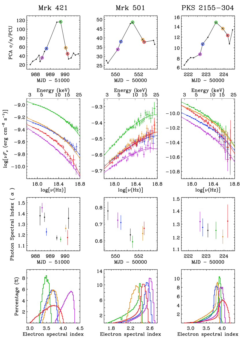
Figure 1: The 3–25 keV PCA light curves, X-ray spectra, photon spectral index variations, and normalized distributions of electron spectral index during a typical flare of Mrk 421, Mrk 501, PKS 2155–304, PKS 2005–489, and 1ES 1959+650, respectively (one column for one source). Top row: 3–25 keV X-ray light curves (typical errors on count rates in units of c/s/PCU are 0.16 for Mrk 421, 0.11 for Mrk 501, 0.09 for PKS 2155-489, 0.08 for PKS 2005–489, and 0.14 for 1ES 1959+650, respectively, which are very small and therefore not plotted). Second row: X-ray spectra with solid curves representing best-fit synchrotron models that were obtained using $\chi^{2}$ statistics (see Table 1). Third row: variations of photon spectral index ($\alpha$) over time during flares. Bottom row: normalized distributions of electron spectral index ($p$) derived with the synchrotron model fitting. For each source (column), the same color represents the same observation.

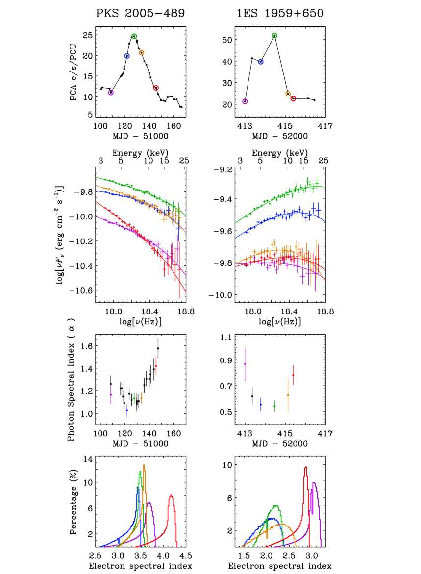
Figure 1 (Cont.):

Figure 2: Light curves (black segmented lines; left y-axis) and evolution of electron spectral index (red segmented lines; right y-axis, which is in the descending order) over time during some typical flares for the five sources. The horizontal segments mark Flares A–L that are further examined in Figure 3.

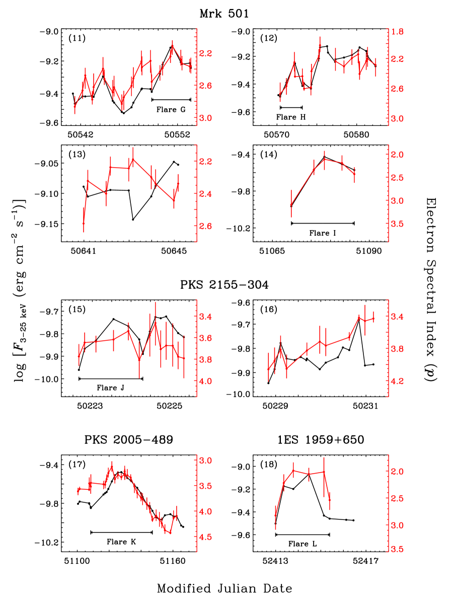
Figure 2 (Cont.):

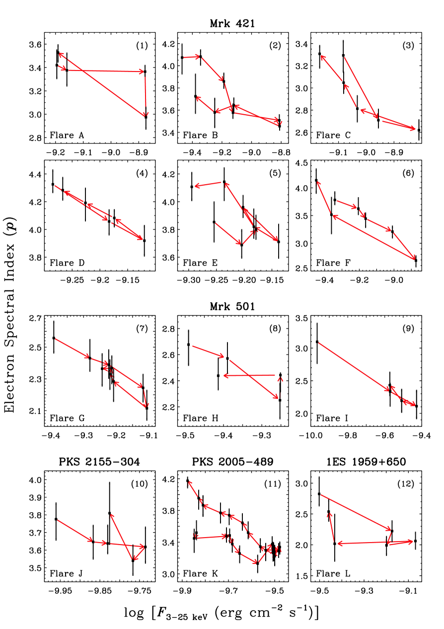
Figure 3: Evolution of electron spectral index ($p$) with flux for the five sources during Flares A–L as annotated in Figure 2, with red arrows indicating time sequences.

4 RESULTS

4.1 X-ray Spectra during Flares

Figure 1 presents one typical flare and its corresponding X-ray spectra during the flare for each of the aforementioned five sources. It shows that the synchrotron radiation model can describe the spectra very well (see the fitting results in Table 2). It is apparent that the X-ray spectrum varies significantly during flares and is harder when flux becomes higher (i.e., harder when brighter), which has been widely studied before: Mrk 421 (e.g., Fossati et al., 2000; Brinkmann et al., 2003; Ravasio et al., 2004; Fossati et al., 2008; Acciari et al., 2011; Baloković et al., 2013; Pian et al., 2014; Aleksić et al., 2015; Kapanadze et al., 2017a), Mrk 501 (e.g., Pian et al., 1998; Krawczynski et al., 2000; Xue & Cui, 2005; Gliozzi et al., 2006; Anderhub et al., 2009; Kapanadze et al., 2017b), 1ES 1959+650 (e.g., Giebels et al., 2002; Kapanadze et al., 2016b, 2018), PKS 2155–304 (e.g., Zhang et al., 2006a, b; Kapanadze et al., 2014; Bhagwan et al., 2016) and PKS 2005–489 (e.g., Perlman et al., 1999).

In the observational energy band (i.e., 3–25 keV shown in Figure 1), the spectral shape is different for the five sources, which indicates that the synchrotron radiation peak is located at different energies. Combining the 3–25 keV spectral shape information and the synchrotron peak energy obtained by fitting all PCA spectra with the log-parabolic model detailed in Section 5.4, we found that: for Mrk 421, the peak energy of all the spectra is below 6 keV, which is consistent with the results in Massaro et al. (2004), Tanihata et al. (2004) and Tramacere et al. (2007) (but Tramacere et al. 2009 shows that its peak energy could be up to 30 keV); for Mrk 501, the peak energy of most spectra is above 3 keV, and Massaro et al. (2008) shows that its peak energy could be up to 100 keV; for PKS 2005–489 and PKS 2155–304, the peak energy of spectra is below 3 keV; for 1ES 1959+650, the peak energy of most spectra is below 30 keV. In fact, it was sometimes difficult to evaluate the exact location of SED peak, which could fall beyond our limited spectral band coverage. Therefore, we could only provide a rough range of peak energy here.

4.2 Electron Spectral Evolution

As we mentioned before, a general trend, which the spectrum hardens with the flux increasing, has been observed in blazars in X-ray observations. There are several conjectures for leading to such a trend. One of them is hardening or softening in the electron spectral distribution. Xue et al. (2006) had demonstrated that variation of electron spectral index ($p$) is indispensable during a flare. They found that the quality of RXTE/PCA spectra enables utilizing the synchrotron model to place reasonable constraints upon $p$ evolution during major flares of two TeV blazars Mrk 421 and Mrk 501, i.e., $p$ variation is required and the electron spectrum tends to be harder/softer with the increase/decrease of flux, in addition to accompanying changes of some other key parameters. We confirm and strengthen the results of Xue et al. (2006), by finding that such a trend of $p$ evolution widely exits in multiple flares of five TeV blazars (see Figures 1 and 2) and variation of $p$ over time is synchronous with variation of flux over time. In addtion, the trend of $p$ evolution is consistent with that of the $\alpha$ evolution (see Figure A1 in the appendix). Noting the fact that the above five TeV blazars are all HBLs, we further examined the behaviours of BL Lacertae (the brightest IBL in Table 1) and 3C 279 (the brightest FSRQ in Table 1) in the $\alpha$-flux plot and found that both of them also show a harder-when-brighter trend.

However, there are a few exceptions that show a complex or even opposite evolution of $p$ rather than the simple harder-when-brighter trend during flares. For example, in panels (6), (9), (13), and (16) of Figure 2, the count-rate light curve and $p$ “light curve” somehow lose track of each other, and thus do not follow the general trend seen in the other panels where $p$ evolution and count-rate evolution generally track each other in a synchronous way. We show the spectra and spectral variations of the case that exhibits the most apparent exception (i.e., panel 13) in Figure B1. These exceptions might be due to the complexity of physical conditions in the emission region and/or the interaction between multiple populations of emitting electrons in two adjacent and comparative flares. For the latter case, the one-zone synchrotron radiation scenario could not be valid and the introduction of multiple populations of emitting electrons might be essential.

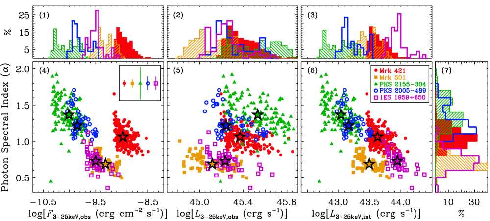
Figure 4: Relations between photon spectral index ($\alpha$) and brightness parameters: observed 3–25 keV X-ray flux ($\textit{F}_{\textrm{3--25keV,obs}}$; panel 4), observed luminosity ($\textit{L}_{\textrm{3--25keV,obs}}$; panel 5) and intrinsic luminosity ($\textit{L}_{\textrm{3--25keV,int}}$ that has been corrected for the Doppler boosting effect using the lower limit of the Doppler factor from Fan et al. 2013; panel 6) for the five sources, respectively. Pentagrams represent median values. The typical errors on $\alpha$ are shown in the inset at the top-right corner of panel (4). The panels of 1, 2, 3 and 7 show histograms of $\textit{F}_{\textrm{3--25keV,obs}}$, $\textit{L}_{\textrm{3--25keV,obs}}$ and $\textit{L}_{\textrm{3--25keV,int}}$, $\alpha$, respectively.

4.3 Electron Spectral Hysteresis

In a conventional hardness-flux plot, spectral hardness can be different in the rising and falling periods of flares, which is known as “spectral hysteresis” and related to both acceleration and cooling timescales. In fact, spectral hysteresis could reveal itself as a “loop” shape in the hardness-flux plot (where the spectrum becomes harder along the positive y-axis direction and the flux becomes higher along the positive x-axis direction). Generally, a “hard lag” should result in a counter-clockwise loop, while a “soft lag” would lead to a clockwise loop (e.g., Abeysekara et al., 2017). X-ray spectral hysteresis has been found in many blazars (e.g., Kataoka et al., 2000; Böttcher & Chiang, 2002; Zhang et al., 2002; Sembay et al., 2002; Cui, 2004; Ravasio et al., 2004; Böttcher & Reimer, 2004; Xue & Cui, 2005; Brinkmann et al., 2005; Gliozzi et al., 2006; Acciari et al., 2009; Tramacere et al., 2009; Kapanadze et al., 2016a, 2017a, 2017b, 2017c; Abeysekara et al., 2017; Kapanadze et al., 2018); and UV-optical spectral hysteresis has also been seen in non-blazar jet knots (e.g., Perlman et al., 2011).

From Figure 2, we further selected a number of flares (i.e., Flares A–L) to examine a different version of spectral hysteresis that is in the form of electron spectral hysteresis (shown as Figure 3), which is consistent with the photon spectral hysteresis (see Figure A2 in the appendix). In many of these $p$-flux plots, electron spectral hysteresis is apparent, rendering itself in a “loop” (e.g., panel 6 of Figure 3 that corresponds to Flare F of Mrk 421), or oblique “8” (e.g., panels of 1, 2, 3, 5, 11, and 12 that correspond to Flares A, B, C, E of Mrk 421, Flare K of PKS 2005–489, and Flare L of 1ES 1959+650, respectively) shape; whereas some cases show no apparent hysteresis (e.g., panels of 4, 7, 8, 9, and 10 that correspond to Flare D of Mrk 421, Flare G, H, I of Mrk 501, and Flare J of PKS 2155–304, respectively), given the relatively large errors of $p$. As in Sections 4.1 and 4.2, most panels of Figures 3 also show an overall trend that electron spectrum typically hardens with flux increasing and softens during decreasing phase, which might reflect a process of electron acceleration, injection, or cooling. Interestingly, there are a few cases that seem to behave in a perplexing way. For instance, for Flare A of Mrk 421 (panel 1), the spectrum starts with almost no spectral variability but a flux increase, then suddenly hardens when flux remains invariable (the flare peak might happen to be between the third and fourth observations of this flare, which was not observed and led to such a case) and softens with a flux decrease; and Flare K of PKS 2005–489 (panel 11) shows that the value of $p$ is nearly invariable during the rising period of the flare, given the uncertainties on $p$. Perlman et al. (1999) had analyzed the prominent flare of PKS 2005–489 (as shown in panel 10 of Figure 3) and found that the 2–10 keV X-ray spectral variability follows a counter-clockwise “loop” in the spectral index-flux plane. The evolution of $p$-flux in this work is consistent with their result.

Electron spectral index ($p$) represents the fraction of electrons in different energies. The fraction of high-energy electrons increases with the value of $p$ decreasing. For most flares in Figure 3, it appears that the value of $p$ in the rise phase of the flare is larger than (panels 2, 3, 6, 7, 8, and 12) or approximately equal to (panels 4 and 9) the value in the decay phase. In other words, at the beginning of the flare, the fraction of high-energy electrons is low and subsequently increases gradually, which leads to “hard lag”. However, for the flares in panels (1), (10), and (11), the trend is opposite; this means that the fraction of high-energy electrons is high in the beginning and then decreases, which leads to “soft lag”. We then used cross-correlation function to search for likely time lags between soft-band (3–8 keV) and hard-band (8–25 keV) light curves, but found no evidence for existence of time lags. These non-detections of time lags might be due to the fact that the actual time lag is likely intra-day, which is difficult to resolve using our light curves of several-day time resolution. In Garson et al. (2010), two flares of Mrk 421 lasting for 0.5 days showed several-hour time lags between the 0.5–2 keV and 2–10 keV light curves, and displayed different movements in the hardness-flux plot. Krawczynski et al. (2000) indicated that the time lag between 3 keV and 25 keV is smaller than 15 hours in Mrk 501. Therefore, more intra-day observational data would be required to detect likely time lags of our sources that might be responsible for the observed electron spectral hysteresis.

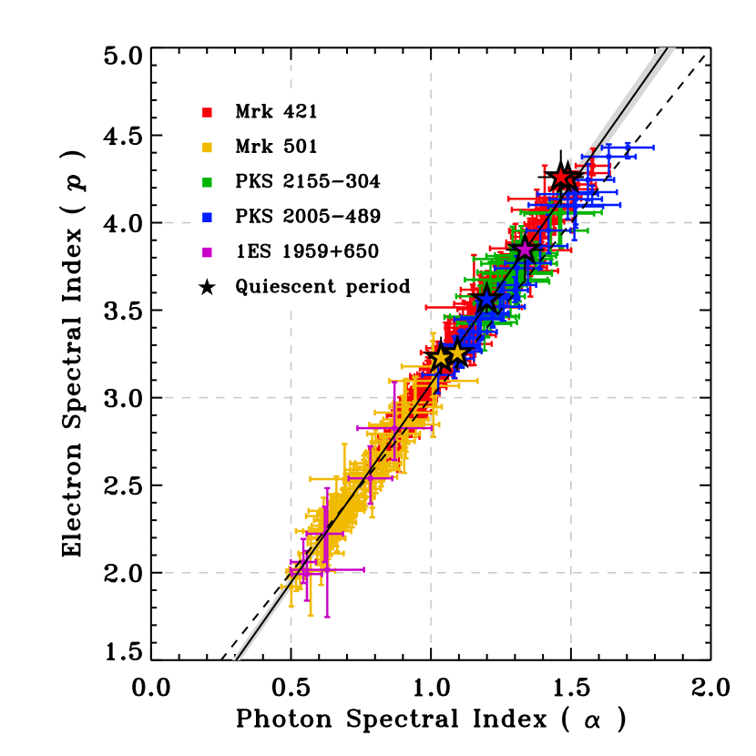
Figure 5: $p$-$\alpha$ (electron spectral index-photon spectral index) relation of the five sources. Colored filled squares represent flaring observations; pentagrams represent quiescent-period observations (see Section 2.3 and Table 2). Squares and pentagrams in the same color represent the same source. The black solid line and its shaded region represent the best fit and 1-$\sigma$ uncertainty to all data of flaring periods, i.e., $p$ = ($2.27\pm 0.03)\times\alpha$ + ($0.81\pm 0.03$). The dashed line indicates the relation of $\alpha=(p-1)/2$ as expected in the optically thin synchrotron radiation spectrum in power-law shape.

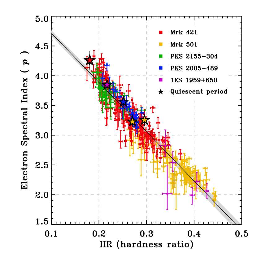
Figure 6: $p$-HR (electron spectral index-hardness ratio) relation of the five sources. All symbols have the same meaning as in Figure 5. The best fit to all data of flaring periods is $p$ = ($-8.28\pm 0.16)\times$HR + ($5.54\pm 0.05$).

4.4 Photon Spectral Index versus Luminosity

As Figure 4 shows, for a single object, photon spectral index ($\alpha$) decreases with increasing flux (panel 4) or luminosity (panels of 5, 6), which is the so-called harder-when-brighter trend (see Section 4.1); while for the entirety of the five sources, photon spectral index seems to increase with increasing observed luminosity (panel 5; see median values denoted by pentagrams), but decrease with increasing intrinsic luminosity that has been corrected for the Doppler boosting effect (panel 6). To control for spectral data quality in Figure 4, we only chose observations with fluxes above 0.25$\times$($\textit{F}_{\textrm{max}}-\textit{F}_{\textrm{min}}$) for each source, where $\textit{F}_{\textrm{max}}$ and $\textit{F}_{\textrm{min}}$ are the maximum and minimum fluxes of the source among the 16-year data, respectively.

The positive correlation between photon spectral index and observed luminosity (panel 5 of Figure 4) is correlated with the “blazar sequence” (Fossati et al., 1998; Ghisellini et al., 1998). According to the blazar sequence, there is a negative correlation between the synchrotron peak energy and the observed bolometric luminosity ($L_{\rm bol}$). The observed bolometric flux can be estimated roughly through the relation of $\textit{F}_{\textrm{bol}}\simeq\textrm{5}\nu_{\textrm{p}}\textit{F}\textrm{(}\nu_{\textrm{p}}\textrm{)}$, where $\nu_{\textrm{p}}\textit{F}\textrm{(}\nu_{\textrm{p}}\textrm{)}$ is the peak flux of the synchrotron hump (Massaro et al., 2004), such that $L_{\rm bol}\simeq 5\nu_{\textrm{p}}L(\nu_{\textrm{p}})\propto L_{\textrm{3--25 keV}}$. In addition, there is an anti-correlation between X-ray photon spectral index and synchrotron peak energy (e.g., Lin et al., 1999; Giommi et al., 2005; Perlman et al., 2005). Therefore, when the peak moves to the lower energy band, the X-ray luminosity will increase and the X-ray spectrum will tend to steepen. As a result, there would be a positive correlation between the X-ray luminosity and X-ray photon spectral index, as demonstrated in the panel (5) of Figure 4 (the Spearman’s ranking correlation for the overall $\alpha$-$L_{\textrm{3--25keV,observed}}$ relation of the five sources is 0.31 with a significance of 3.42 $\times\textrm{10}^{\textrm{--13}}$). However, the anti-correlation between synchrotron peak energy and luminosity (the blazar sequence) dispears after applying Doppler boosting correction to the observed luminosity (e.g., Nieppola et al., 2008; Wu et al., 2009; Huang et al., 2014; Fan et al., 2017). In this work, we performed approximate Doppler-corrections using the equation $\textit{L}_{\textrm{intrinsic}}=\textit{L}_{\textrm{observed}}/\delta^{3}$, where $\textit{L}_{\textrm{intrinsic}}$ is the intrinsic luminosity, $\textit{L}_{\textrm{observed}}$ is the observed luminosity and $\delta$ is the lower limit of the $\gamma$-ray Doppler factor from Fan et al. (2013) that is estimated according to the pair-production optical depth (Mattox et al., 1993): 2.77 for Mrk 421, 2.83 for Mrk 501, 4.15 for PKS 2155–304, 3.30 for PKS 2005–489 and 2.32 for 1ES 1959+650. Our results are consistent with the previous studies (panel 6 of Figure 4): the Spearman’s ranking correlation for the overall $\alpha$-$L_{\textrm{3--25keV,intrinsic}}$ relation of the five sources is –0.46 with a significance of 2.33$\times\textrm{10}^{\textrm{--28}}$.

5 DISCUSSION

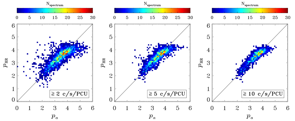
Figure 7: Density maps of $p_{\rm HR}$-$p_{\alpha}$ distribution ($p_{\rm HR}$ and $p_{\alpha}$ estimated using the $p$-HR and $p$-$\alpha$ relations, respectively) for all HBL spectra in three different count-rate regimes, respectively. Black solid lines represent $y=x$. Color bars atop indicate numbers of HBL spectra contained within a pixel.

5.1 Electron Spectral Index versus Photon Spectral Index

We obtained the photon spectral index ($\alpha$) by fitting spectra with the cut-off power law model rather than the log-parabolic model. These two models both provided great spectral fitting results, but the photon spectral index in the log-parabolic model is energy dependent, so we did not adopt $\alpha$ from this model. The cut-off power law model follows the relation of $F(E)\propto E^{-\alpha}\cdot\exp{(-E/\beta)}$, where $\beta$ is the e-folding energy of exponential roll-off. In this work, we have assumed that the electron spectral distribution follows the power-law shape, which usually produces the optically thin synchrotron radiation spectrum with a power-law photon spectral index of $\alpha$ = $(p-\textrm{1})/\textrm{2}$ (see the dashed line in Figure 5). However, in this work, the cut-off power-law model could provide better fits to all the spectra than the power-law model; therefore, we used the cut-off power law model to obtain photon spectral index ($\alpha$).

According to Figure 5, there is a significant linear relation between $p$ and $\alpha$ during flares of the five sources, which follows the formula of

$$p=(2.27\pm 0.03)\times\alpha+(0.81\pm 0.03).$$ (1)

This relation shows a slight deviation from the theoretical relation of $\alpha$ = $(p-\textrm{1})/\textrm{2}$ for the power-law spectral distribution. This deviation might be due to the energy loss of electrons and acceleration process of relativistic electrons, which could produce the spectrum not exactly following the power-law distribution. Therefore, for the X-ray spectrum not following the power-law shape, it might not be suitable to use $\alpha$ = $(p-\textrm{1})/\textrm{2}$ to calculate $p$ using $\alpha$ and vice versa.

In addition, values of $p$ and $\alpha$ in relatively quiescent periods (i.e., pentagrams in Figure 5) seem to follow nicely the above $p$-$\alpha$ relation that was derived with flaring periods, which indicates that the spectra during flaring and quiescent periods share the same $p$-$\alpha$ relation.

5.2 Electron Spectral Index versus Hardness Ratio

We define hardness ratio (HR) as HR = H$/$S, where H and S are count rates in the 8–25 keV and 3–8 keV bands, respectively. As expected, Figure 6 also presents a linear relation between $p$ and HR during flares, which follows the formula of

$$p=(-8.28\pm 0.16)\times\textrm{HR}+(5.54\pm 0.05).$$ (2)

We had verified that a similar linear relation between $p$ and HR${}_{(\textrm{10}\textrm{-}\textrm{25})\textrm{keV}/(\textrm{3}\textrm{-}\textrm{10})\textrm{keV}}$ would also be obtained, which is not presented here. The $p$-HR relation (i.e., Eq. 2) is not as tight as the $p$-$\alpha$ relation (i.e., Eq. 1), and the former has significantly larger scatters than the latter, which is also expected given the following two facts: the derivation of $\alpha$ makes use of full spectral information while the calculation of HR only utilizes crude spectral information; and the influence of Galactic absorption was not taken into account for deriving HR, which should introduce additional small scatters. Furthermore, values of $p$ and HR in relatively quiescent periods (i.e., pentagrams in Figure 6) also seem to generally follow the $p$-HR relation that was derived with flaring periods (cf. Section 5.1 and Figure 5).

5.3 Application of $p$-$\alpha$ and $p$-HR Relations

The $p$-$\alpha$ and $p$-HR relations provide us two quick and straightforward empirical approaches to roughly estimate the electron spectral index ($p$) simply based on values of $\alpha$ and/or HR, without resorting to detailed synchrotron radiation modeling. The distribution of $p$ can only be obtained through fitting spectra with the synchrotron radiation model, which not only relies on high-quality spectral data, but also takes a long time. Therefore, if one is only interested in knowing the approximate range of $p$ for a particular spectrum, then it would be efficient to estimate $p$ using one of the $p$-$\alpha$ and $p$-HR relations or even both.

For the purpose of verifying the reliability of these two approaches, we compared values of $p$ estimated using $\alpha$ with that estimated using HR, utilizing all HBL spectral data among the 32 TeV blazars (note that the 3–25 keV spectra of FSRQs, LBLs, and IBLs might be dominated by both synchrotron and inverse Compton scattering components, which are not suitable for simple synchrotron radiation modeling). Figure 7 shows a reasonably good agreement between $p_{\alpha}$ and $p_{\textrm{HR}}$ that were derived using the $p$-$\alpha$ and $p$-HR relations, respectively. As the flux increases, the estimation of $p$ becomes more reliable, leading to an improved agreement between $p_{\alpha}$ and $p_{\textrm{HR}}$, thanks to the better quality of data. Therefore, although the $p$-HR relation shows a larger scatter compared with the $p$-$\alpha$ relation, it is still a reliable way to estimate $p$ quickly.

One thing worth noting is that there is a nearly horizontal low-density tail to the top of the distribution. We excluded the likely “pileup”-like effect for this feature because the fluxes of these observations are not very high. The possible reason is that $p$-$\alpha$ and $p$-HR relations do not completely follow the linear correlation, i.e., the $p$ derived from the data is smaller than the best-fit $p$-$\alpha$ relation at $\alpha$ $>$ 1.5 (see Figure 5) and is larger than the best-fit $p$-HR relation at HR $<$ 0.2 (see Figure 6). Therefore, if we use the best-fit relations to estimate the $p$ in the high $p$ range, the $p_{\alpha}$ tends to be larger and the $p_{\textrm{HR}}$ tends to be smaller, which will lead to a nearly horizontal tail. Even so, for the vast majority of observations, $p$-$\alpha$ and $p$-HR relations can provide consistent $p$ estimates.

As demonstrated above, both the $p$-$\alpha$ and $p$-HR relations are suitable for estimation of $p$ in the case that the radiative process is dominated by synchrotron radiation in jets. We note that the $p$-HR relation should be instrument-dependent because HR is closely related to the instrument response, therefore being valid only for RXTE/PCA data; while the $p$-$\alpha$ relation should be instrument-independent.

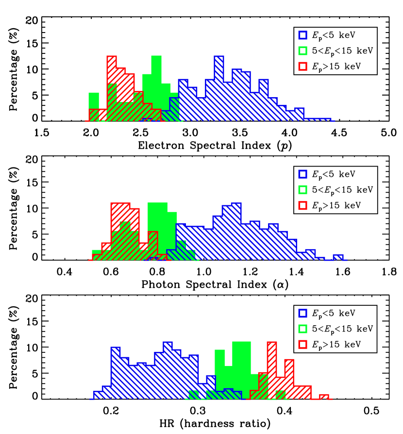
Figure 8: Distributions of electron spectral index, photon spectral index, and hardness ratio for all spectra of flaring periods, which are divided into three groups according to their peak energies ($E_{\rm p}$) of synchrotron radiation humps (blue, green, and red histograms for $E_{\rm p}<5$ keV, 5 keV$<E_{\rm p}<$15 keV, and $E_{\rm p}>$15 keV, respectively).

5.4 Peak Energy versus Spectral Parameters

For many cases in blazars, the log-parabolic model could greatly reproduce the spectra around the synchrotron peak in the SED, which provides a valid method to estimate the energy and flux of the peak (e.g., Massaro et al., 2004; Tanihata et al., 2004; Tramacere et al., 2007, 2009). Therefore, we used the log-parabolic model to estimate $\textit{E}_{\textrm{p}}$ following Massaro et al. (2004), which is given by

$$\textit{F(E)}=\textit{K}(\textit{E}/\textit{E}_{1})^{(-\textit{a}+\textit{b}\log(\textit{E}/\textit{E}_{1}))}\ \ \bigl{(}\textrm{ph}\ \textrm{cm}^{\textrm{--2}}\ \textrm{s}^{\textrm{--1}}\ \textrm{keV}^{\textrm{--1}}\bigr{)}.$$ (3)

$\textit{E}_{\textrm{1}}$ is the reference energy that is generally fixed to 1 keV, a is the photon spectral index at the energy of $\textit{E}_{\textrm{1}}$, b is the curvature parameter, and K is the normalization factor. The values of these parameters can be derived from the spectral fitting process. The peak energy of synchrotron radiation hump is given by $\textit{E}_{\textrm{p}}^{\textrm{obs}}=\textit{E}_{\textrm{1}}\textrm{10}^{(\textrm{2}-\textit{a})/\textrm{2}\textit{b}}.$ The rest-frame peak energy is $\textit{E}_{\textrm{p}}=(1+\emph{z})\textit{E}_{\textrm{p}}^{\textrm{obs}}$, where z is the redshift. In some cases, parameter b is below 0, which means that the fitted curve is concave, and the resulting peak energy is not the real peak energy of synchrotron hump. There are many reasons for such a result, such as a concave spectrum and poor quality of data (especially in the high-energy band). For such cases, we could only obtain a rough range of $\textit{E}_{\textrm{p}}$: if b $<$ 0 and $\textit{E}_{\textrm{p,fit}}$ $<$ 3 keV, then $\textit{E}_{\textrm{p}}$ $>$ 25 keV or $\textit{E}_{\textrm{p}}$ $<$ 3 keV; if b $<$ 0 and $\textit{E}_{\textrm{p,fit}}$ $>$ 3 keV, then $\textit{E}_{\textrm{p}}$ $<$ 3 keV ($\textit{E}_{\textrm{p,fit}}$ is the fitting result of the peak energy). Fortunately, there are only two observations with b $<$ 0 and both of them belong to the second case.

For the flaring periods of the five sources, according to the location of synchrotron radiation SED peak, we roughly divided a total of 276 spectra into three groups: $\textit{E}_{\textrm{p}}$ $<$ 5 keV (202 spectra), 5 keV $<$ $\textit{E}_{\textrm{p}}$ $<$ 15 keV (32 spectra), and $\textit{E}_{\textrm{p}}$ $>$ 15 keV (42 spectra). Figure 8 presents the distributions of three spectral parameters $p$, $\alpha$, and HR for these three groups of spectra. Although our sample is not complete, it still reveals a general trend that, with the synchrotron radiation SED peak energy increasing, both $p$ and $\alpha$ decrease while HR increases. This is consistent with the trend that the spectra are harder with higher peak frequencies seen in other works (e.g., Lin et al., 1999; Giommi et al., 2005; Perlman et al., 2005).

Additionally, some rough constraints upon $\textit{E}_{\textrm{p}}$ (also see Section 4.1) and the three spectral parameters can be obtained, according to Figure 8: if $\textit{E}_{\textrm{p}}$ is lower than 5 keV, then $p$ is higher than $\sim$ 2.7, $\alpha$ is higher than $\sim$ 0.8, and HR is lower than $\sim$ 0.35; if $\textit{E}_{\textrm{p}}$ is higher than 5 keV, then $p$ is lower than $\sim$ 3.0, $\alpha$ is lower than $\sim$ 1.0, and HR is higher than $\sim$ 0.30. The constrained range of $\alpha$ is in good agreement with the result in Perlman et al. (2005), where three hard ($\Gamma$ $<$ 2, i.e., $\alpha$ $<$ 1) spectra correspond to $\textit{E}_{\textrm{p}}$ $>$ 5 keV.

6 SUMMARY AND CONCLUSIONS

During its entire lifespan ($\sim$ 16 years), RXTE had observed 32 TeV blazars, including 2 FSRQs, 1 LBLs, 5 IBLs, and 24 HBLs. In this paper, we analyzed the 16-year RXTE/PCA observational data of the 32 TeV blazars and further selected out five brightest sources to carry out a systematic investigation of X-ray spectral variability during their major flares in the RXTE era, using both empirical spectral fitting (to obtain values of $\alpha$, flux and $E_{\rm p}$) and theoretical synchrotron radiation modeling (to obtain $p$ distributions). Our work builds on Xue et al. (2006) that studied only two TeV blazars, confirms and strengthens their main results with a larger sample, and provides many further insights regarding X-ray spectral variability of TeV blazars. We summarize our main results as follows:

1. The cut-off power-law and log-parabolic models could provide evenly good fitting results to the X-ray spectra of all sources. The X-ray spectra, characterized by $\alpha$, display a harder-when-brighter trend during a number of flares of the five brightest sources (i.e., Mrk 421, Mrk 501, PKS 2155–304, PKS 2005–489, and 1ES 1959+650), which is consistent with previous studies.

2. The high quality of the PCA data of the five sources enables detailed synchrotron radiation modeling upon their spectra. It seems clear that the evolution of $p$ also generally follows a harder-when-brighter trend; and the variation of $p$, accompanied by changes of other key parameters, is required to explain the observed X-ray spectral variability of TeV blazars during flares, which would have useful implications for interpreting the associated higher-energy (i.e., gamma-ray) spectral variability that the same population of ultra-relativistic electrons are responsible for. These results confirm and strengthen that of Xue et al. (2006). However, there are some cases that do not follow the harder-when-brighter trend exactly, which might be related to the complex physical conditions in the emitting region or the “contamination” of electron populations from adjacent flares.

3. Electron spectral hysteresis is clearly seen in many but not all $p$-flux plots, rendering itself in a “loop” or oblique “8” shape. Although this phenomenon is often associated with time lags between the soft and hard bands, no apparent hard or soft lag is identified based on our several-day-timescale light curves. Intra-day observations might help resolve likely intra-day time lags.

4. A tight $p$-HR relation and a tighter $p$-$\alpha$ relation are obtained using spectra of flaring periods, both of which are also applicable to stacked data of quiescent periods, indicating that both relations are independent of flux level. These two relations can be used to estimate $p$ quickly and straightforwardly, and the reliability of $p$ estimation improves as improved data quality.

5. Collectively (i.e., TeV blazars being treated as a whole), $\alpha$ and X-ray luminosity are positively correlated, $E_{\rm p}$ is negatively correlated with $p$ and $\alpha$, and $E_{\rm p}$ is positively correlated with HR. All these correlations are in line with the blazar sequence. However, after correcting for the Doppler boosting effect, $\alpha$ and intrinsic X-ray luminosity follow an anti-correlation.

Appendix A photon spectral evolution and photon spectral hysteresis

In Figures 2 and 3, we have shown the electron spectral evolution and electron spectral hysteresis, respectively. Given that most of the previous works studied spectral variability through photon spectral index, in this appendix we also show the photon spectral evolution in Figure A1 and photon spectral hysteresis in Figure A2. The photon spectral evolution shows a harder-when-brighter trend (see Figure A1), which is consistent with previous studies, and also shows a similar trend to that revealed by $p$ evolution (see Figure 2). In addition, the photon spectral hysteresis (see Figure A2) shows a similar trend to that seen with electron spectral hysteresis (see Figure 3). Therefore, consistent results on spectral evolution and hysteresis are obtained using either the $\alpha$ or $p$ representation, which is expected given the tight $p$–$\alpha$ relation (see Figure 5).

Appendix B opposite evolution of spectral index with flux

During the period between MJD 50641 and 50645 (i.e., panel 13 of Figure 2), Mrk 501 shows a softer-when-brighter trend in terms of $p$ variation, which is opposite to the harder-when-brighter trend existing in most of the studied cases (see Figure 2 and Section 4.2). The spectra and $\alpha$ variations of these observations are showed in Figure B1, which also show a softer-when-brighter trend. Several cases also present a similar opposite trend, e.g., Mrk 421 in the period between MJD 54509 and 54511 (see panel 6), and PKS 2155–304 in the period between MJD 50229.2 and 50230.2 (see panel 16). This opposite trend of these three cases exists in the transition region between two individual flares, which indicates that it might be due to the interaction between multiple populations of emitting electrons in the two adjacent flares.

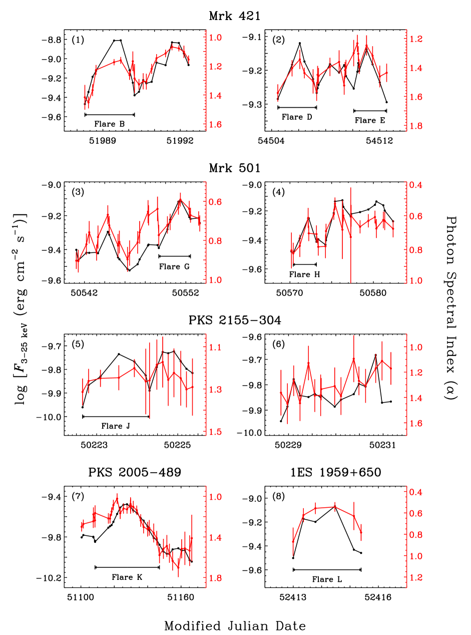
Figure A1: Same as Figure 2, but for the evolution of photon spectral index ($\alpha$; red segmented lines; right y-axis). The $\alpha$ evolution shows a harder-when-brighter trend, similar to the $p$ evolution. For brevity, only 8 panels of Figure 2 are re-plotted here for demonstration, as all panels give the same result.

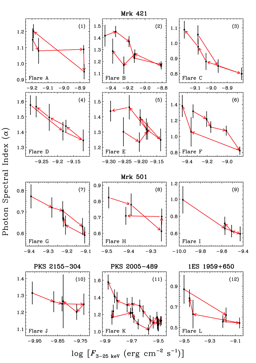
Figure A2: Same as Figure 3, but for the evolution of photon spectral index ($\alpha$).

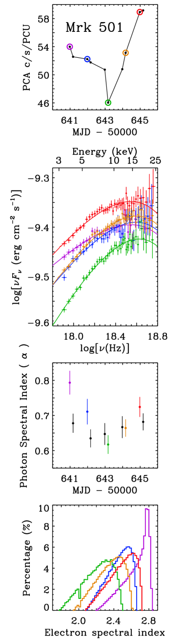
Figure B1: Same as Figure 1, but for Mrk 501 during the period between MJD 50641 and 50645 (cf. panel 13 of Figure 2).

References

- Abdo et al. (2010a) Abdo, A. A., Ackermann, M., Agudo, I., et al. 2010a, ApJ, 716, 30
- Abdo et al. (2010b) Abdo, A. A., Ackermann, M., Ajello, M., et al. 2010b, ApJ, 710, 1271
- Abeysekara et al. (2017) Abeysekara, A. U., Archambault, S., Archer, A., et al. 2017, ApJ, 834, 2
- Acciari et al. (2011) Acciari, V. A., Aliu, E., Arlen, T., et al. 2011, ApJ, 738, 25
- Acciari et al. (2009) Acciari, V. A., Aliu, E., Aune, T., et al. 2009, ApJ, 703, 169
- Aharonian (2000) Aharonian, F. A. 2000, New A, 5, 377
- Aleksić et al. (2015) Aleksić, J., Ansoldi, S., Antonelli, L. A., et al. 2015, A&A, 576, A126
- Anderhub et al. (2009) Anderhub, H., Antonelli, L. A., Antoranz, P., et al. 2009, ApJ, 705, 1624
- Arnaud (1996) Arnaud, K. A. 1996, Astronomical Data Analysis Software and Systems V, 101, 17
- Atoyan & Dermer (2003) Atoyan, A. M., & Dermer, C. D. 2003, ApJ, 586, 79
- Böttcher & Reimer (2004) Böttcher, M., & Reimer, A. 2004, ApJ, 609, 576
- Böttcher et al. (2013) Böttcher, M., Reimer, A., Sweeney, K., & Prakash, A. 2013, ApJ, 768, 54
- Böttcher & Chiang (2002) Böttcher, M., & Chiang, J. 2002, ApJ, 581, 127
- Baloković et al. (2013) Baloković, M., Ajello, M., Blandford, R. D., et al. 2013, European Physical Journal Web of Conferences, 61, 04013
- Bhagwan et al. (2016) Bhagwan, J., Gupta, A. C., Papadakis, I. E., & Wiita, P. J. 2016, New A, 44, 21
- Boettcher et al. (1997) Boettcher, M., Mause, H., & Schlickeiser, R. 1997, A&A, 324, 395
- Brinkmann et al. (2003) Brinkmann, W., Papadakis, I. E., den Herder, J. W. A., & Haberl, F. 2003, A&A, 402, 929
- Brinkmann et al. (2005) Brinkmann, W., Papadakis, I. E., Raeth, C., Mimica, P., & Haberl, F. 2005, A&A, 443, 397
- Cui (2004) Cui, W. 2004, ApJ, 605, 662
- Dermer et al. (1992) Dermer, C. D., Schlickeiser, R., & Mastichiadis, A. 1992, A&A, 256, L27
- Dickey & Lockman (1990) Dickey, J. M., & Lockman, F. J. 1990, ARA&A, 28, 215
- Fan et al. (2016) Fan, J. H., Yang, J. H., Liu, Y., et al. 2016, ApJS, 226, 20
- Fan et al. (2017) Fan, J. H., Yang, J. H., Xiao, H. B., et al. 2017, ApJ, 835, L38
- Fan et al. (2013) Fan, J.-H., Yang, J.-H., Liu, Y., & Zhang, J.-Y. 2013, Research in Astronomy and Astrophysics, 13, 259
- Fossati et al. (2008) Fossati, G., Buckley, J. H., Bond, I. H., et al. 2008, ApJ, 677, 906
- Fossati et al. (2000) Fossati, G., Celotti, A., Chiaberge, M., et al. 2000, ApJ, 541, 166
- Fossati et al. (1998) Fossati, G., Maraschi, L., Celotti, A., Comastri, A., & Ghisellini, G. 1998, MNRAS, 299, 433
- Fraija & Marinelli (2015) Fraija, N., & Marinelli, A. 2015, Astroparticle Physics, 70, 54
- Garson et al. (2010) Garson, A. B., III, Baring, M. G., & Krawczynski, H. 2010, ApJ, 722, 358
- Ghisellini et al. (1998) Ghisellini, G., Celotti, A., Fossati, G., Maraschi, L., & Comastri, A. 1998, MNRAS, 301, 451
- Giannios et al. (2009) Giannios, D., Uzdensky, D. A., & Begelman, M. C. 2009, MNRAS, 395, L29
- Giebels et al. (2002) Giebels, B., Bloom, E. D., Focke, W., et al. 2002, ApJ, 571, 763
- Giommi et al. (1990) Giommi, P., Barr, P., Garilli, B., Maccagni, D., & Pollock, A. M. T. 1990, ApJ, 356, 432
- Giommi et al. (2005) Giommi, P., Piranomonte, S., Perri, M., & Padovani, P. 2005, A&A, 434, 385
- Gliozzi et al. (2006) Gliozzi, M., Sambruna, R. M., Jung, I., et al. 2006, ApJ, 646, 61
- Harris et al. (2003) Harris, D. E., Biretta, J. A., Junor, W., et al. 2003, ApJ, 586, L41
- Harris et al. (2006) Harris, D. E., Cheung, C. C., Biretta, J. A., et al. 2006, ApJ, 640, 211
- Hinshaw et al. (2013) Hinshaw, G., Larson, D., Komatsu, E., et al. 2013, ApJS, 208, 19
- Holder (2014) Holder, J. 2014, Brazilian Journal of Physics, 44, 450
- Huang et al. (2014) Huang, B., Zhang, X., Xiong, D., & Zhang, H. 2014, Journal of Astrophysics and Astronomy, 35, 381
- Inoue & Tanaka (2016) Inoue, Y., & Tanaka, Y. T. 2016, ApJ, 818, 187
- Kapanadze et al. (2017a) Kapanadze, B., Dorner, D., Romano, P., et al. 2017a, ApJ, 848, 103
- Kapanadze et al. (2017b) Kapanadze, B., Dorner, D., Romano, P., et al. 2017b, MNRAS, 469, 1655
- Kapanadze et al. (2016a) Kapanadze, B., Dorner, D., Vercellone, S., et al. 2016a, ApJ, 831, 102
- Kapanadze et al. (2018) Kapanadze, B., Dorner, D., Vercellone, S., et al. 2018, MNRAS, 473, 2542
- Kapanadze et al. (2014) Kapanadze, B., Romano, P., Vercellone, S., & Kapanadze, S. 2014, MNRAS, 444, 1077
- Kapanadze et al. (2016b) Kapanadze, B., Romano, P., Vercellone, S., et al. 2016b, MNRAS, 457, 704
- Kapanadze et al. (2017c) Kapanadze, S., Kapanadze, B., Romano, P., Vercellone, S., & Tabagari, L. 2017c, Ap&SS, 362, 196
- Kataoka et al. (2000) Kataoka, J., Takahashi, T., Makino, F., et al. 2000, ApJ, 528, 243
- Kirk et al. (1998) Kirk, J. G., Rieger, F. M., & Mastichiadis, A. 1998, A&A, 333, 452
- Krawczynski et al. (2000) Krawczynski, H., Coppi, P. S., Maccarone, T., & Aharonian, F. A. 2000, A&A, 353, 97
- Lin et al. (1999) Lin, Y. C., Bertsch, D. L., Bloom, S. D., et al. 1999, ApJ, 525, 191
- Lyutikov (2003) Lyutikov, M. 2003, New A Rev., 47, 513
- Mücke & Protheroe (2001) Mücke, A., & Protheroe, R. J. 2001, Astroparticle Physics, 15, 121
- Mücke et al. (2003) Mücke, A., Protheroe, R. J., Engel, R., Rachen, J. P., & Stanev, T. 2003, Astroparticle Physics, 18, 593
- Maraschi et al. (1992) Maraschi, L., Ghisellini, G., & Celotti, A. 1992, ApJ, 397, L5
- Marshall et al. (2002) Marshall, H. L., Miller, B. P., Davis, D. S., et al. 2002, ApJ, 564, 683
- Massaro et al. (2004) Massaro, E., Perri, M., Giommi, P., & Nesci, R. 2004, A&A, 413, 489
- Massaro et al. (2008) Massaro, F., Tramacere, A., Cavaliere, A., Perri, M., & Giommi, P. 2008, A&A, 478, 395
- Mastichiadis & Kirk (1997) Mastichiadis, A., & Kirk, J. G. 1997, A&A, 320, 19
- Mattox et al. (1993) Mattox, J. R., Bertsch, D. L., Chiang, J., et al. 1993, ApJ, 410, 609
- Nieppola et al. (2008) Nieppola, E., Valtaoja, E., Tornikoski, M., Hovatta, T., & Kotiranta, M. 2008, A&A, 488, 867
- Padovani & Giommi (1995) Padovani, P., & Giommi, P. 1995, ApJ, 444, 567
- Perlman et al. (2011) Perlman, E. S., Adams, S. C., Cara, M., et al. 2011, ApJ, 743, 119
- Perlman et al. (2005) Perlman, E. S., Madejski, G., Georganopoulos, M., et al. 2005, ApJ, 625, 727
- Perlman et al. (1999) Perlman, E. S., Madejski, G., Stocke, J. T., & Rector, T. A. 1999, ApJ, 523, L11
- Pian et al. (2014) Pian, E., Türler, M., Fiocchi, M., et al. 2014, A&A, 570, A77
- Pian et al. (1998) Pian, E., Vacanti, G., Tagliaferri, G., et al. 1998, ApJ, 492, L17
- Ravasio et al. (2004) Ravasio, M., Tagliaferri, G., Ghisellini, G., & Tavecchio, F. 2004, A&A, 424, 841
- Rees (1978) Rees, M. J. 1978, MNRAS, 184, 61P
- Rivers et al. (2013) Rivers, E., Markowitz, A., & Rothschild, R. 2013, ApJ, 772, 114
- Rivers et al. (2011) Rivers, E., Markowitz, A., & Rothschild, R. 2011, ApJS, 193, 3
- Sambruna et al. (1994) Sambruna, R. M., Barr, P., Giommi, P., et al. 1994, ApJ, 434, 468
- Sembay et al. (2002) Sembay, S., Edelson, R., Markowitz, A., Griffiths, R. G., & Turner, M. J. L. 2002, ApJ, 574, 634
- Sikora et al. (1994) Sikora, M., Begelman, M. C., & Rees, M. J. 1994, ApJ, 421, 153
- Spada et al. (2001) Spada, M., Ghisellini, G., Lazzati, D., & Celotti, A. 2001, MNRAS, 325, 1559
- Sushch & H. E. S. S. Collaboration (2015) Sushch, I., & H. E. S. S. Collaboration 2015, Advances in Astronomy and Space Physics, 5, 59
- Tanihata et al. (2004) Tanihata, C., Kataoka, J., Takahashi, T., & Madejski, G. M. 2004, ApJ, 601, 759
- Tramacere et al. (2009) Tramacere, A., Giommi, P., Perri, M., Verrecchia, F., & Tosti, G. 2009, A&A, 501, 879
- Tramacere et al. (2007) Tramacere, A., Massaro, F., & Cavaliere, A. 2007, A&A, 466, 521
- Urry & Padovani (1995) Urry, C. M., & Padovani, P. 1995, PASP, 107, 803
- Wu et al. (2009) Wu, Z.-Z., Gu, M.-F., & Jiang, D.-R. 2009, Research in Astronomy and Astrophysics, 9, 168
- Xue & Cui (2005) Xue, Y., & Cui, W. 2005, ApJ, 622, 160
- Xue et al. (2006) Xue, Y., Yuan, F., & Cui, W. 2006, ApJ, 647, 194
- Zhang et al. (2006a) Zhang, Y. H., Bai, J. M., Zhang, S. N., et al. 2006a, ApJ, 651, 782
- Zhang et al. (2002) Zhang, Y. H., Treves, A., Celotti, A., et al. 2002, ApJ, 572, 762
- Zhang et al. (2006b) Zhang, Y. H., Treves, A., Maraschi, L., Bai, J. M., & Liu, F. K. 2006b, ApJ, 637, 699
- Zhu et al. (2018) Zhu, S. F., Xue, Y. Q., Brandt, W. N., Cui, W., & Wang, Y. J. 2018, ApJ, 853, 34