Perfect anomalous transport of subdiffusive cargos by molecular motors in viscoelastic cytosol

Abstract

Multiple experiments show that various submicron particles such as magnetosomes, RNA messengers, viruses, and even much smaller nanoparticles such as globular proteins diffuse anomalously slow in viscoelastic cytosol of living cells. Hence, their sufficiently fast directional transport by molecular motors such as kinesins is crucial for the cell operation. It has been shown recently that the traditional flashing Brownian ratchet models of molecular motors are capable to describe both normal and anomalous transport of such subdiffusing cargos by molecular motors with a very high efficiency. This work elucidates further an important role of mechanochemical coupling in such an anomalous transport. It shows a natural emergence of a perfect subdiffusive ratchet regime due to allosteric effects, where the random rotations of a “catalytic wheel” at the heart of the motor operation become perfectly synchronized with the random stepping of a heavily loaded motor, so that only one ATP molecule is consumed on average at each motor step along microtubule. However, the number of rotations made by the catalytic engine and the traveling distance both scale sublinearly in time. Nevertheless, this anomalous transport can be very fast in absolute terms.

I Introduction

Intracellular transport by molecular motors is crucial for a eukaryotic cell operation (Pollard et al. (2008), Phillips et al. (2013), Nelson (2003)). This is especially true in view of the recent discoveries (Luby-Phelps (2013)) that various nanoparticle probes (Saxton and Jacobson (1997), Guigas et al. (2007)), as well as naturally occurring biological nanoparticles such as proteins (Weiss et al. (2004), Banks and Fradin (2005), Weigel et al. (2011)), viruses (Seisenberger et al. (2001)), RNA messengers (Golding and Cox (2006)), various endosomes and granulates (Tolic-Norrelykke et al. (2004), Jeon et al. (2011), Caspi et al. (2002), Bruno et al. (2011), Tabei et al. (2013)), including artificial magnetosomes (Robert et al. (2010)), and also lipids (Kneller et al. (2011), Jeon et al. (2012)) subdiffuse either in membrane or in cytosol of living cells. This means that the mean-square distance covered by such particles scales sublinearly in time, $\langle\delta r^{2}(t)\rangle\sim 2D_{\alpha}t^{\alpha}/\Gamma(1+\alpha)$, where $\alpha$ is a power law exponent of subdiffusion, $0<\alpha<1$, $D_{\alpha}$ is subdiffusion coefficient (within an effective 1d description), and $\Gamma(z)$ is familiar gamma-function. For example, magnetosomes of radius about $R=300$ nm subdiffuse in intact cytosol of PC3 tumor cells with $\alpha\approx 0.4$, and $D_{\alpha}\approx 170\;{\rm nm^{2}/s^{0.4}}$, see in Robert et al. (2010), Goychuk et al. (2014b), Goychuk (2015). To subdiffuse over the distance of $2R$, such an endosome would require about $2.705\times 10^{7}$ seconds or about 313 days. Clearly a passive transport of such particles by subdiffusion on any significant distance within the cell is just impossible on any physiologically relevant time scale. However, some cells must solve the tasks such as e.g. delivery of ion channels in a transfer bag provided by an endosome on the distances which can be even meter long, as e.g. in axons of some neuronal cells (Hirokawa and Takemura (2005)). So, how can cells solve such tasks even using an active transport by such molecular motors as kinesins, if cytosol is a gel-like viscoelastic medium causing subdiffusion? In particular, can such a transport be normal, rather than anomalously slow, in the sense that the traveling distance along the cell’s microtubuli highways scales not sublinearly in time, $\langle\delta r(t)\rangle\sim t^{\alpha_{\rm eff}}$, with some $\alpha\leq\alpha_{\rm eff}<1$, what is expected, but simply linearly with $\alpha_{\rm eff}=1$. Can such a transport be effective and sufficiently fast? And how? These are some challenging questions to be answered.

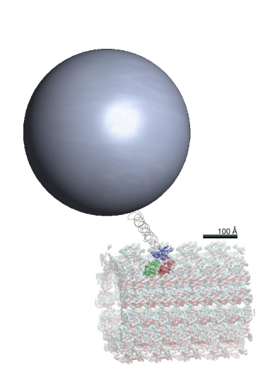
Figure 1: Kinesin walking on microtubule and pulling cargo on an elastic tether.

Figure 2: More realistic biochemical cycle for one motor head (left) and the minimal two-state model of cycling (right) that includes a binding potential change due to a change of the charge state of the motor. Spatial dependence of the transition rates on the coordinate along a periodic polar background of microtubule provides an allosteric mechanism of the mechano-chemical coupling.

The simplest modeling of a molecular motor is to represent it by a constant pulling force $F$ acting on a cargo, which, otherwise, thermally subdiffuses (Caspi et al. (2002)), when it is not coupled to the motor. When the motor walks on microtubuli constituting a random transport network (kinesins), or it changes its walking direction at random along the same track (myosins), the motor action on its cargo can be modeled by a fluctuating, non-thermal random force $F(t)$ (Caspi et al. (2002), Bruno et al. (2009)). In the absence of motors, thermal subdiffusion in viscoelastic media is described by a generalized Langevin equation or GLE (Mason and Weitz (1995), Amblard et al. (1996), Waigh (2005)), with a memory friction and thermal random force obeying the thermal fluctuation dissipation theorem (FDT), Kubo (1966), Zwanzig (2001). An algebraically slow memory decay $\propto t^{-\alpha}$ yields subdiffusion $\langle\delta r^{2}(t)\rangle\sim t^{\alpha_{\rm eff}}$, with $\alpha_{\rm eff}=\alpha$, in the absence of non-thermal $F(t)$. The motor-driven diffusion has another exponent $\beta$, $\langle\delta r^{2}(t)\rangle\propto t^{\beta}$, with the maximal value $\beta_{\rm max}=2\alpha$ (Bruno et al. (2009)) within this model. It can be superdiffusive only for $\alpha>0.5$. However, an experiment by Robert et al. (2010) in a medium with e.g. $\alpha=0.4$ yielded $\beta=1.3\pm 0.1$ of active motor-assisted transport. It is essentially larger than $2\alpha=0.8$. Also another experiment by Harrison et al. (2013) yielded $\beta\approx 1.74$ for the active transport with $\alpha\approx 0.58$ of the passive transport. Hence, such a modeling is far too simple and it cannot explain these experimental findings. A different modeling route of flashing Brownian ratchets (Astumian and Bier (1996), Jülicher et al. (1997), Parmeggiani et al. (1999)) was taken by Goychuk et al. (2014a, b), Goychuk (2015, 2016). It is based on an extension of the previous research work on normal diffusion Brownian ratchets, see e.g. review by Reimann (2002), onto the case of viscoelastic subdiffusion featured by long-range memory correlations in the medium (Goychuk (2009, 2012b)). Such kind of subdiffusion naturally emerges in dense polymeric solutions, colloidal liquids and glasses, as well as cytosol of living cells (Larson (1999), Waigh (2005), Mason and Weitz (1995), Amblard et al. (1996), Gittes et al. (1997), Santamaría-Holek et al. (2007), Pan et al. (2009), Weiss (2013)). A recent work by Goychuk (2018) explains how this kind of subdiffusion can win over the medium’s disorder also featuring such complex heterogeneous media as cytosol.

Rocking ratchets of normal diffusion (Magnasco (1993), Doering et al. (1994), Bartussek et al. (1994)) have been generalized to viscoelastic subdiffusion by Goychuk (2010), Goychuk and Kharchenko (2012, 2013), Kharchenko and Goychuk (2013), and flashing ratchets (Ajdari and Prost (1992), Prost et al. (1994), Rousselet et al. (1994), Astumian and Bier (1994)) by Kharchenko and Goychuk (2012). The first application of flashing subdiffusive ratchets to molecular motors pulling nanocargos was done by Goychuk et al. (2014a). In that work, motor and cargo make one subdiffusing quasi-particle in assumptions that a tether between them is infinitely rigid, and a spatially-asymmetric periodic ratchet potential acting on the motor stochastically switches between two realizations differing by a half of the spatial period shift, like in Makhnovskii et al. (2004). Moreover, Markovian switching rates are identical and constant. Two such subsequent switches make one random cycle. The mechano-chemical coupling is neglected in that earlier model. Depending on the size of cargo determining the subdiffusion coefficient of combined quasi-particle, frequency of the binding potential flashing, loading force applied, and other parameters, both anomalous and normal transport regimes can be realized, Goychuk et al. (2014a). Very important is that the ratchet transport of a subdiffusive cargo can be perfectly normal, in the sense that each switching cycle results on average in the transport step on a distance of the spatial period, and the averaged number of such switches grows linearly in time (a perfect normal ratchet). However, anomalous transport regimes can also be readily enforced. This model provides a principal framework to explain the origin of $\beta=1.3\pm 0.1$ for $\alpha=0.4$ in Robert et al. (2010), and also the origin of $\beta\approx 1.74$ in Harrison et al. (2013), where the passive subdiffusion of lipid droplets with $\alpha\approx 0.58$ is changed to superdiffusion induced and assisted by molecular motors.

The tether or linker between the motor and its cargo is, however, never infinitely rigid and the motor walking on microtubule is not fully exposed to viscoelastic constituents of cytosol. For this reason, Goychuk et al. (2014b) considered a more involved model with the motor being normally diffusing in a ratchet potential of a similar kind (although, a different, saw-tooth form of the binding ratchet potential has been chosen), whereas the cargo is subdiffusing in viscoelastic cytosol, and both particles are connected by some elastic linker, like in Fig. 1. Major earlier results were confirmed within this more realistic model, which still lacked, however, a mechano-chemical coupling between the mechanical motion of the motor and cargo and the biochemical cycling of the motor in its intrinsic conformational space. This drawback has been overcome by Goychuk (2015) who considered a very similar, in general features, model for the motor as one by Astumian and Bier (1996), Jülicher et al. (1997), Parmeggiani et al. (1999). It takes the mechano-chemical coupling into account, and also the fact that any tether must have a finite maximal extension length. The related nonlinear effects were shown to be important, Goychuk (2015), for weak tethers like one in Bruno et al. (2011). This model is general and rich enough. It permits different specific models for the mechano-chemical coupling, Parmeggiani et al. (1999). One chosen by Goychuk (2015) (model A in this paper) allowed to closely reproduce the earlier results in Goychuk et al. (2014b) for the same amplitude of the ratchet potential, $U_{0}=0.5\;{\rm eV}=20\;{k_{B}T_{r}}$. In this particular case, the mechano-chemical coupling is effectively absent, and the motors perform cyclic turnovers with one almost fixed, position-independent rate for a very similar set of parameters as in the earlier work, Goychuk et al. (2014b). However, already for $U_{0}=25\;{k_{B}T_{r}}$ and $U_{0}=30\;{k_{B}T_{r}}$ larger than the free energy of ATP hydrolysis, $\Delta G_{\rm ATP}=20\;{k_{B}T_{r}}$, used to drive one biochemical cycle of the motor, the effects of mechano-chemical coupling become also very essential in the model A. The most striking effect is that the number of motor turnovers and the number of ATP molecules hydrolyzed during its operation start to scale sublinearly in time, $\langle N_{turn}(t)\rangle\propto t^{\gamma}$, with $\alpha_{\rm eff}\leq\gamma\leq 1$. For the ratchet model with constant rates, $\gamma=1$ always. Since the work against an external loading force scales as $t^{\alpha_{\rm eff}}$ and the energy consumed as $t^{\gamma}$, the thermodynamic efficiency generally decays in time as $1/t^{\lambda}$ with $\lambda=\gamma-\alpha_{\rm eff}$, Goychuk (2015). However, it can be appreciably large, over 50% for a rather long time period (at the end of simulations corresponding to about 3 sec of physical time and traveling distances of the order of micrometer) at the maximum sub-power of operation (Goychuk (2015, 2016)). This regime requires, however, a large $U_{0}>\Delta G_{\rm ATP}$, with the stalling force about $10$ pN (for $U_{0}=30\;{k_{B}T_{r}}$, Goychuk (2015)). It is essentially larger than $5$ pN or $5.5-6.5$ pN observed for kinesins by Svoboda et al. (1993), and Schnitzer et al. (2000), respectively.

The major question we address in this work is whether a similar regime is possible also for $U_{0}=\Delta G_{\rm ATP}=20\;k_{B}T_{r}$, and the stalling force in the range from 5 to 6 pN, as observed experimentally. It will be shown that such a regime indeed emerges, however, for a different model of mechano-chemical coupling (the model B below and in Parmeggiani et al. (1999)) such that it cannot be reduced to a ratchet model with constant switching rates in some range of parameters (like it happens within the model A). Moreover, the emergence of a perfect subdiffusive ratchet regime will be manifested with $\gamma=\alpha_{\rm eff}<1$, where thermodynamic efficiency does not decay in time. Such a perfect anomalous synchronization between anomalous biochemical turnovers of molecular motor and its mechanical motion due to a mechano-chemical coupling leads to a transport efficiency of nearly 100%, where consumption of one ATP molecule results into one step of the motor loaded with cargo along microtubule.

II Methods, Theory and Simulations

We consider a model based on one studied earlier (Astumian and Bier (1996), Jülicher et al. (1997), Parmeggiani et al. (1999), Goychuk et al. (2014a, b)). In essence, this is the same model as in Goychuk (2015). Molecular motor moves in a flashing periodic saw-tooth ratchet potential, $U(x+L,\zeta(t))=U(x,\zeta(t))$, like one in the graphical abstract, with some potential height $U_{0}$. Here, $L=8$ nm is the spatial period of microtubule, Pollard et al. (2008), Phillips et al. (2013), Svoboda et al. (1993), and $\zeta(t)$ is a conformational state of the motor. Microtubuli are well-known to be polar, overally negatively charged periodic structures, Baker et al. (2001), which provide transport highways for such motors as kinesins, Pollard et al. (2008). Hence, emergence of a periodic and asymmetric potential for charged nanoparticles, like molecular motor-proteins attached to microtubule, is quite natural. Furthermore, ATP molecules which serve as the source of free energy for the motors like kinesins or myosins, are also (negatively) charged, like are the products of the ATP hydrolysis: ADP and the phosphate group $P_{i}$. Thus, it is very natural that the binding potential flashes upon the conformational change of the motor related to its charge state fluctuations. The biochemistry of kinesin operation is very complex as it has two heads, with a simplest biochemical cycle depicted in the left part of Fig. 2. The simplest theoretical model for its cycling is given in the right part of Fig. 2 (Hill (1989), Astumian and Bier (1996), Jülicher et al. (1997)). This is a biochemical two-cycle or bi-cycle, with some four lump rates. Of course, it presents a gross over-simplification, and hence, a truly minimal theoretical model. These rates are spatially-dependent, which expresses a mechano-chemical coupling, see below. In the spirit of this two-state model, one considers only two conformations, $\zeta_{1}$ and $\zeta_{2}$, with $\zeta(t)$ undergoing two-state fluctuations with spatially-dependent rates. Since two subsequent flashes make one cycle with the potential shifted by one spatial period, and the both motor heads are identical, it is natural to impose $U(x+L/2,\zeta_{1})=U(x,\zeta_{2})$ as an additional symmetry condition within this minimal model. Likewise, not only $\alpha_{1,2}(x+L)=\alpha_{1,2}(x)$, $\beta_{1,2}(x+L)=\beta_{1,2}(x)$, but also $\alpha_{1,2}(x+L/2)=\beta_{2,1}(x)$, etc. in this model. Furthermore, the energy $\Delta G_{\rm ATP}$ is used to rotate the “catalytic wheel” (Wyman (1975), Rozenbaum et al. (2004), Qian (2005)) in one preferred (counter-clockwise in Fig. 2) direction. Thermodynamically this implies (Hill (1989), Qian (2005))

$$\frac{\alpha_{1}(x)\beta_{2}(x)}{\alpha_{2}(x)\beta_{1}(x)}=\exp[\Delta G_{\rm ATP}/(k_{B}T)],$$ (1)

for any $x$, what can be satisfied, e.g., by choosing

$$\frac{\alpha_{1}(x)}{\alpha_{2}(x)} = \exp[(U_{1}(x)-U_{2}(x)+\Delta G_{\rm ATP}/2)/(k_{B}T)],$$

$$\frac{\beta_{1}(x)}{\beta_{2}(x)} = \exp[(U_{1}(x)-U_{2}(x)-\Delta G_{\rm ATP}/2)/(k_{B}T)].$$ (2)

Furthermore, the total rates

$$\nu_{1}(x) = \alpha_{1}(x)+\beta_{1}(x),$$

$$\nu_{2}(x) = \alpha_{2}(x)+\beta_{2}(x)$$ (3)

of the transitions between two energy profiles must satisfy

$$\frac{\nu_{1}(x)}{\nu_{2}(x)}=\exp[(U_{1}(x)-U_{2}(x))/(k_{B}T)]$$ (4)

at thermal equilibrium. This is condition of the thermal detailed balance, where the dissipative fluxes vanish both in the transport direction and within the conformational space of motor, at the same time (Jülicher et al. (1997), Astumian and Bier (1996)). It is obviously satisfied for $\Delta G_{\rm ATP}\to 0$. There is still a lot of freedom in choosing rates, within the imposed requirements. One possibility is to fix some $\alpha_{1}(x)=\beta_{2}(x+L/2)$. Then,

$$\nu_{1}(x) = \alpha_{1}(x+L/2)\exp\left[-\frac{U_{2}(x)-U_{1}(x)+\Delta G_{\rm ATP}/2}{k_{B}T}\right]$$ (5)

$$+ \alpha_{1}(x),$$

$$\nu_{2}(x) = \alpha_{1}(x)\exp\left[-\frac{U_{1}(x)-U_{2}(x)+\Delta G_{\rm ATP}/2}{k_{B}T}\right]$$

$$+ \alpha_{1}(x+L/2)\;.$$

This is our model A. Another choice is to fix $\alpha_{2}(x)=\beta_{1}(x+L/2)$. Then,

$$\nu_{1}(x) = \alpha_{2}(x)\exp\left[\frac{U_{1}(x)-U_{2}(x)+\Delta G_{\rm ATP}/2)}{k_{B}T}\right]$$ (6)

$$+ \alpha_{2}(x+L/2),$$

$$\nu_{2}(x) = \alpha_{2}(x+L/2)\exp\left[\frac{U_{2}(x)-U_{1}(x)+\Delta G_{\rm ATP}/2)}{k_{B}T}\right]$$

$$+ \alpha_{2}(x)\;.$$

provides our model B, which is similar to the model B by Parmeggiani et al. (1999). In both models, we shall assume that either $\alpha_{1}(x)=const$, or $\alpha_{2}(x)=const$, correspondingly, in a $\pm\delta/2$ neighborhood of the minimum of potential $U_{1}(x)$, and is zero otherwise. Using $\delta$ appropriately, $\delta=L/2$ in this paper, one can ensure that the enzyme turnovers can occur everywhere on microtubule, and not in some specially chosen domains only. The difference between the models A and B seems subtle. However, the results are rather different, see below. In particular, the mechano-chemical coupling is markedly stronger in the model B.

The mechanical motion of the motor is mimicked by a Brownian particle subjected to the force $f(x,\zeta(t))=-\partial U(x,\zeta(t))/\partial x$ coming from the binding potential, viscous friction force $-\eta_{m}\dot{x}$, and a thermal white Gaussian noise $\xi_{m}(t)$. The latter two are related by the second FDT, $\langle\xi_{m}(t)\xi_{m}(t^{\prime})\rangle=2k_{B}T\eta_{m}\delta(t-t^{\prime})$ at the environmental temperature $T$. Inertial effects are neglected, like in the previous studies of molecular motors. Indeed, dynamics of nanoparticles in polymeric water solutions is typically overdamped. The inertial effects are present typically on the initial scales from picoseconds to nanoseconds, and we are interested in much longer times, up to seconds and minutes. Furthermore, the motor is assumed to be elastically coupled to a cargo (within a FENE model, Herrchen and Öttinger (1997), Goychuk (2015)), with a spring constant $\kappa_{L}$ and a maximal extension length $r_{max}$. The limit $r_{max}\to\infty$ corresponds to a harmonic linker. Moreover, the motor is generally subjected also to a constant loading force $f_{0}$, which attempts to stop its directional motion being counter-directed. All in all, the motor is described by Eq. (7) in

$$\eta_{m}\dot{x} = f(x,\zeta(t))-f_{0}+\xi_{m}(t)+\frac{\kappa_{L}(y-x)}{1-(y-x)^{2}/r_{\rm max}^{2}},$$ (7)

$$\eta_{c}\dot{y} = -\int_{0}^{t}\eta_{\rm mem}(t-t^{\prime})\dot{y}(t^{\prime})dt^{\prime}$$

$$- \frac{\kappa_{L}(y-x)}{1-(y-x)^{2}/r_{\rm max}^{2}}+\xi_{c}(t)+\xi_{\rm mem}(t)\;.$$

$f(x,\zeta(t))$ is piece-wise constant within the model considered. With the maximum of $U(x)$ dividing the potential period in the ratio $1:p$, $p>1$, it takes negative value $f_{-}=-(p+1)U_{0}/L$ within the spatial interval $[0,L/(p+1))$ and positive value $f_{+}=(p+1)U_{0}/(pL)$ within the larger interval $[L/(p+1),L)$. Here, $U(0)=U(L)=0$. If flashing is sufficiently slow, so that the particle has time to relax to the potential minimum after each potential flash, it will be pushed forward by $f_{+}$ to a new potential minimum after each flash. In this way, a perfect ratchet transport mechanism can be realized, if flashing is also not far too slow, so that the particle does not have enough time to escape to another potential minimum being thermally agitated. For a high potential barrier $U_{0}\gg k_{B}T$, such escapes occur, however, very infrequently. With an increasing loading force $f_{0}$, the potential barrier diminishes and it vanishes at $f_{\rm st}=f_{+}$, which is the stalling force in the absence of thermal fluctuations at $T=0$. It must be mentioned, however, in this respect that at physiological temperatures the stalling force depends strongly on temperature. To obtain it, $U_{0}$ should be replaced with a free energy barrier $U_{0}\to F_{0}=U_{0}-TS$, with $S\approx 11.2\;k_{B}$ for $\alpha_{1}=170\;s^{-1}$ within the model A, Goychuk et al. (2014b), Goychuk (2015). The entropic component is as large as $T_{r}S\approx 11.2\;k_{B}T_{r}$ at $T_{r}=290$ K. Hence, to get a realistic stalling force for kinesin from 5 to 6 pN, Svoboda et al. (1993), or about $7$ pN (Kojima et al. (1996)) at room temperatures, $U_{0}$ should be about $20\;k_{B}T_{r}$, or somewhat larger. For $U_{0}<15\;k_{B}T_{r}$, the above simple estimate does not work, cf. Fig. 6 in Goychuk et al. (2014b), and the stalling force is far too small, as compared to the experimental values.

Also elastic coupling to the cargo will generally strongly affect the motor operation. The cargo motion is described by Eq. (A.1). It is subjected both to the viscous friction with the friction coefficient $\eta_{c}$ reflecting about 80% of water content in cytosol, and to a viscoelastic memory friction characterized by the memory kernel $\eta_{\rm mem}(t)$. These frictional terms are related to the corresponding components of the thermal noise of the environment by the Kubo’s second FDT, named also the fluctuation-dissipation relation or FDR, Kubo (1966), Zwanzig (2001), Weiss (1999), $\langle\xi_{c}(t)\xi_{c}(t^{\prime})\rangle=2k_{B}T\eta_{c}\delta(t-t^{\prime}),\langle\xi_{\rm mem}(t)\xi_{\rm mem}(t^{\prime})\rangle=k_{B}T\eta_{\rm mem}(|t-t^{\prime}|)$. Viscoelasticity with a complex shear modulus $G^{*}(\omega)\propto(i\omega)^{\alpha}$ (Mason and Weitz (1995), Waigh (2005), Larson (1999)) corresponds to a strictly sub-Ohmic memory kernel, $\eta_{\rm mem}(t)=\eta_{\alpha}t^{-\alpha}/\Gamma(1-\alpha)$, $0<\alpha<1$, Weiss (1999), with fractional friction coefficient $\eta_{\alpha}$, Goychuk (2009, 2012b). The corresponding memory term can be abbreviated as $\eta_{\alpha}d^{\alpha}y/dt^{\alpha}$ using the notion of fractional Caputo derivative (Gorenflo and Mainardi (1997), Mathai and Haubold (2017)). Furthermore, the corresponding thermal noise $\xi_{\rm mem}(t)$ is fractional Gaussian noise (fGn). It is a time derivative of the fractional Brownian motion (fBm) by Kolmogorov (1940, 1991), Mandelbrot and van Ness (1968). When the cargo is uncoupled to the motor ($\kappa_{L}=0$), spread of its position variance is described by

$$\langle\delta y^{2}(t)\rangle=2D_{c}tE_{1-\alpha,2}\left(-[t/\tau_{\rm in}]^{1-\alpha}\right),$$ (9)

see in Kharchenko and Goychuk (2013), where $E_{a,b}(z)=\sum_{n=0}^{\infty}z^{n}/\Gamma(an+b)$ is the generalized Mittag-Leffler function (Mathai and Haubold (2017)), and $D_{c}=k_{B}T/\eta_{c}$ is normal diffusion coefficient. Initially, at $t\ll\tau_{\rm in}=(\eta_{c}/\eta_{\alpha})^{1/(1-\alpha)}$ diffusion is normal, $\langle\delta y^{2}(t)\rangle\approx 2D_{c}t$ whereas at large times, $t\gg\tau_{\rm in}$, it is anomalously slow, $\langle\delta y^{2}(t)\rangle\approx 2D_{\alpha}t^{\alpha}/\Gamma(1+\alpha)$. Here, $D_{\alpha}=k_{B}T/\eta_{\alpha}$ is the fractional diffusion coefficient whose value plays a key role in anomalous transport processes.

II.1 Markovian embedding

Seen realistically, any power-law memory kernel has a long-time memory cutoff. Assuming it being exponential, $\eta_{\alpha}\to\eta_{\alpha}\exp(-\nu_{h}t)$, an effective friction coefficient $\eta_{\rm eff}=\int_{0}^{\infty}\eta_{\rm mem}(t)dt=\eta_{\alpha}\tau_{\rm max}^{1-\alpha}$ can be introduced with $\tau_{\rm max}=1/\nu_{h}$. For $t\gg\tau_{\rm max}$, diffusion will be again normal with the diffusion coefficient $D_{c,\rm eff}=k_{B}T/(\eta_{c}+\eta_{\rm eff})$. However, $\tau_{\rm max}$ can be very large, in the range from tens of seconds to hours, see e.g. Table I in Goychuk (2012a) (for a different model of memory cutoff). Furthermore, a short-time memory cutoff $\tau_{\rm min}=1/\nu_{0}$ must also always exist on physical grounds, in any realistic description of a condensed medium beyond the continuous medium approximation. Here, $\nu_{0}$ is related to a maximal frequency of the mediums oscillators coupled to the Brownian particle within a dynamical theory of Brownian motion, Weiss (1999). Hence, it is natural to approximate a power-law-scaling memory kernel between two memory cutoffs by a sum of exponentials,

$$\eta_{\rm mem}(t)=\sum_{i=1}^{N}k_{i}\exp(-\nu_{i}t),$$ (10)

obeying fractal scaling $\nu_{i}=\nu_{0}/b^{i-1}$, $k_{i}=C_{\alpha}(b)\eta_{\alpha}\nu_{i}^{\alpha}/\Gamma(1-\alpha)\propto\nu_{i}^{\alpha}$, where $C_{\alpha}(b)$ is some constant, which depends on $\alpha$ and $b$, Palmer et al. (1984), Hughes (1995), Goychuk (2009, 2012b) Obviously, $\tau_{\rm max}=b^{N-1}/\nu_{0}$. Depending on $b$ and $\alpha$, the accuracy of approximation can be between 4% ($b=10$, $\alpha=0.5$) and 0.01% ($b=2$, $\alpha=0.5$), see in Goychuk and Kharchenko (2013). In fact, it provides an almost optimal approximation to the power law dependence, which can be slightly improved further, as suggested by Bochud and Challet (2007). Upon the use of the Prony series expansion (10), the non-Markovian dynamics of cargo allows for a multi-dimensional Markovian embedding, Goychuk (2012b), by introducing auxiliary Brownian quasi-particles mimicking viscoelastic modes of environment with coordinates $y_{i}$ and frictional coefficients $\eta_{i}=k_{i}/\nu_{i}$. It reads

$$\eta_{c}\dot{y} = -\frac{\kappa_{L}(y-x)}{1-(y-x)^{2}/r_{\rm max}^{2}}-\sum_{i=1}^{N}k_{i}(y-y_{i})$$

$$+ \sqrt{2\eta_{c}k_{B}T}\xi_{0}(t),$$

$$\eta_{i}\dot{y_{i}} = k_{i}(y-y_{i})+\sqrt{2\eta_{i}k_{B}T}\xi_{i}(t),$$ (12)

where $\xi_{i}(t)$ are uncorrelated white Gaussian noises of unit intensity, $\langle\xi_{i}(t^{\prime})\xi_{j}(t)\rangle=\delta_{ij}\delta(t-t^{\prime})$, which are also uncorrelated with the white Gaussian noise sources $\xi_{0}(t)$ and $\xi_{m}(t)$. To have a complete equivalence with the stated GLE model in Eqs. (7), (A.1) with memory kernel (10), the initial positions $y_{i}(0)$ are sampled from independent Gaussian distributions centered around $y(0)$, $\langle y_{i}(0)\rangle=y(0)$ with variances $\langle[y_{i}(0)-y(0)]^{2}\rangle=k_{B}T/k_{i}$, Goychuk (2012b). To see this equivalence, one has to (i) rewrite (A.1) in terms of viscoelastic force $u_{i}=k_{i}(y_{i}-y)$, (ii) formally solve the resulting equation for $u_{i}(t)$ with $\dot{y}(t)$ and $\xi_{i}(t)$ considered formally as some time-dependent functions and (iii) substitute the result, which consists of a regular part corresponding to friction with an exponentially decaying memory and a noise, into Eq. (II.1). Each noise component depends on $u_{i}(0)$, and all noise components are mutually independent. Considering $u_{i}(0)$ as random Gaussian variables with $\langle u_{i}(0)\rangle=0$ and $\langle u_{i}^{2}(0)\rangle=k_{i}k_{B}T$, one can show that the resulting noise $\xi_{\rm mem}(t)$ is indeed a wide sense stationary Gaussian stochastic process which satisfies FDR with the memory function (10), see in Goychuk (2009, 2012b) for detail. The resulting $\xi_{\rm mem}(t)$ presents a sum of independent Ornstein-Uhlenbeck processes which approximates fGn between two memory cutoffs. Langevin equations (7), (II.1), (A.1) considered together with a time-inhomogeneous Markovian process $\zeta(t)$, which is fully defined by two rates $\nu_{1,2}(x(t))$, provide a stochastic-dynamical description of the studied model. It is used in numerics, as described in the Supplementary Material.

Table 1: Parameter sets

Set, Model	$D_{0.4}$, ${\rm nm^{2}/s^{0.4}}$	$\alpha_{2}$, $\rm{s}^{-1}$	$\alpha_{1}$, $\rm{s}^{-1}$	$U_{0}$, $k_{B}T_{r}$	$r_{\rm rmax}$, nm
$S_{1},A$	171		170	20	$\infty$
$S_{2}$, A	1710		170	20	$\infty$
$S_{5}$, A	171		34	20	$\infty$
$S_{7}$, A	171		170	25	80
$S_{8}$, A	171		170	30	80
$S_{9}$, A	1710		170	25	80
$S_{10}$, A	1710		170	30	80
$S_{1}$, B	171	170		20	$\infty$
$S_{2}$, B	1710	170		20	$\infty$
$S_{5}$, B	1710	34		20	$\infty$
$S_{6}$, B	171	17		20	$\infty$
$S_{7}$, B	1710	17		20	$\infty$

II.2 Choice of parameters and the details of numerics

Like in Goychuk et al. (2014b), Goychuk (2015), we use $a_{m}=100$ nm for the effective radius of kinesin, about 10 times larger than its linear geometrical size (without tether) in order to account for the enhanced effective viscosity experienced by the motor partially exposed to cytosol compared to its value in water. The viscous friction coefficient is estimated from the Stokes formula as $\eta_{m}=6\pi a_{m}\zeta_{w}$, where $\zeta_{w}=1\;{\rm mPa\cdot s}$ is water viscosity used in calculations. Furthermore, the time is scaled in the units $\tau_{m}=L^{2}\eta_{m}/U_{0}^{*}$ with $U_{0}^{*}=10\;k_{B}T_{r}$. For the above parameters, $\tau_{m}\approx 2.94\;\mu{\rm s}$. Distance is scaled in units of $L$, elastic coupling constants in units of $U_{0}^{*}/L^{2}\approx 0.64$ pN/nm, and forces in units of $U_{0}^{*}/L\approx 5.12$ pN. $\nu_{0}=100$ ($3.4\cdot 10^{7}$ 1/s) was chosen which corresponds to $\tau_{\rm min}=29.4$ ns, and $\alpha$ was $\alpha=0.4$, as found experimentally in Robert et al. (2010), Bruno et al. (2011). Two cargo sizes were considered, large $a_{c}=300$ nm, which corresponds to the magnetosome size in Robert et al. (2010), and a ten times smaller one, like in Fig. 1. For larger cargo, we assume that its effective Stokes friction $\eta_{c}=6\pi a_{c}\zeta_{w}$ is enhanced by the factor of $\eta_{\rm eff}/\eta_{c}=3\cdot 10^{4}$ in cytosol. A particular embedding with $b=10$ and $N=10$ was chosen in accordance with our previous studies. With these parameters, $\tau_{\rm max}=10^{9}\tau_{\rm min}=29.4$ s and fractional friction coefficient $\eta_{\alpha}=\eta_{\rm eff}\tau_{\rm max}^{\alpha-1}/r$ with $r\approx 0.93$, Goychuk et al. (2014b). The corresponding subdiffusion coefficient is $D_{0.4}=k_{B}T/\eta_{0.4}\sim 1.71\cdot 10^{-16}\;{\rm m^{2}/s^{0.4}}=171\;{\rm nm^{2}/s^{0.4}}$, in a semi-quantitative agreement with the experimental results in Robert et al. (2010). Smaller cargo is characterized by $\eta_{\rm eff}/\eta_{c}=3\cdot 10^{3}$ yielding $D_{0.4}=1710\;{\rm nm^{2}/s^{0.4}}$, ten times larger. Furthermore, within the model A we used two values of the rate constant $\alpha_{1}$: $170\;\rm{s}^{-1}$ (fast) and $34\;\rm{s}^{-1}$ (slow), in order to match approximately the enzyme turnover rates $\nu\sim\alpha_{1}/2$ in Ref. Goychuk et al. (2014b). Accordingly, we used mostly $U_{0}=20$ $k_{B}T_{r}$ in simulations, however, also two larger values of $U_{0}$ were used, see Table 1, in order to arrive at the thermodynamic efficiencies larger than 50%. Within the model B we used three values of $\alpha_{2}$, see in Table 1. The elastic spring constant is fixed to $\kappa_{L}=0.32$ pN/nm in this paper. A similar value was found in experiment, Kojima et al. (1996). For the maximal extension of linker we used $r_{\rm rmax}=80$ nm, Pollard et al. (2008), and also $r_{\rm rmax}=\infty$, which corresponds to harmonic linker in Goychuk et al. (2014b). As it has been shown earlier in Goychuk (2015), for a strong linker considered, the harmonic approximation is, in principle, sufficient. Hence, within the model B in this paper we used only it. However, for weak linkers anharmonic effects can be very essential (Goychuk (2015)). Such weak linkers are not considered in this paper. The studied set of parameters is shown in Table 1.

To numerically integrate stochastic Langevin dynamics for a fixed potential realization $U_{1,2}(x)$, we used stochastic Heun method, see in the Supplementary Material, implemented in parallel on NVIDIA Kepler graphical processors. Stochastic switching between two potential realizations is simulated using a well-known algorithm. Namely, if the motor is moving on $U_{1}(x)$ or $U_{2}(x)$ surface, at each integration time step $\Delta t$ it can switch with the probability $\nu_{1}(x)\Delta t$ or $\nu_{2}(x)\Delta t$, correspondingly, to another state, or to evolve further on the same potential surface. Here, $\nu_{1,2}(x)$ are the rates corresponding to either model A, or model B, see above. We used $\Delta t=5\cdot 10^{-3}$ for the integration time step and $n=10^{3}$ for the ensemble averaging. The maximal time range of integration was $10^{6}$, which corresponds to $2.94$ sec of motor operation. Notice that a further increase of $N$ does not influence results, whereas it exponentially increases $\eta_{\rm eff}$ of cargos. This means that $\eta_{\alpha}$ and $D_{\alpha}$ are the truly relevant parameters of fractional transport, and not $\eta_{\rm eff}$,. Furthermore, $\Delta G_{\rm ATP}=20$ $k_{B}T_{r}$ was taken in all numerical simulations, and $T=T_{r}=290$ K, so that $k_{B}T_{r}\approx 25$ meV.

II.3 Stochastic energetics

Stochastic energetics can be considered following Jülicher et al. (1997), Goychuk (2015). The useful work done by motor against a loading force $f_{0}$ is $W_{\rm use}(t)=f_{0}\langle\delta x(t)\rangle\propto t^{\alpha_{\rm eff}}$, whereas the input energy that it consumes scales as $E_{\rm in}(t)=\Delta G_{\rm ATP}\langle N_{\rm turn}(t)\rangle$, where $\langle N_{\rm turn}(t)\propto t^{\gamma}$ is the number of turnovers $1\to 2\to 1$. This yields for thermodynamic efficiency

$$R_{\rm th}(t)=\frac{W_{\rm use}(t)}{\Delta G_{\rm ATP}\langle N_{\rm turn}(t)\rangle}\propto 1/t^{\gamma-\alpha_{\rm eff}}.$$ (13)

This definition is, however, not quite precise because it assumes that all the turnovers of the “catalytic wheel” occur with ATP hydrolysis. However, some turnovers occur backwards, with ATP synthesis, within this model. Since such backward turnovers occur seldomly for $\Delta G_{\rm ATP}=0.5$ eV, Eq. (13) only slightly underestimates the proper efficiency, see in Goychuk (2015). To correctly calculate consumption of ATP molecules one should count $p_{1}\Delta G_{\rm ATP}/2$, with $p_{1}=(\alpha_{1}-\beta_{1})/(\alpha_{1}+\beta_{1})$ for the transition $U_{1}\to U_{2}$, and $p_{2}\Delta G_{\rm ATP}/2$ with $p_{2}=(\beta_{2}-\alpha_{2})/(\alpha_{2}+\beta_{2})$ for the transition $U_{2}\to U_{1}$. A corresponding modification of (13) will be named the proper efficiency.

III Results

Table 2: Parameters of the fit with Eq. (21) within 1% error tolerance done with the Levenberg-Marquardt algorithm using XMGRACE software, Turner (2005), and the corresponding values of $R_{\rm th}^{(\rm max)}$, and $f_{\rm max}$.

Set, Model	$k$	$f_{\rm st}$, pN	$\epsilon$	$q$	$R_{\rm th}^{(\rm max)}$	$f_{\rm max}$, pN
$S_{1},A$	0.389	6.00	1.270	0.923	0.103	3.06
$S_{2}$, A	0.447	5.89	2.032	-1.251	0.237	4.15
$S_{5}$, A	0.458	4.81	3.447	0.653	0.194	2.88
$S_{7}$, A	0.823	9.05	1.152	0.307	0.284	5.18
$S_{8}$, A	0.968	9.98	0.761	-40.44	0.707	8.50
$S_{9}$, A	0.872	9.04	7.140	-0.111	0.580	6.92
$S_{10}$, A	0.973	10.0	4.780	-23.24	0.828	9.16
$S_{1}$, B	0.387	6.30	4.966	0.993	0.103	3.12
$S_{2}$, B	0.606	6.29	6.981	0.707	0.331	4.16
$S_{5}$, B	0.525	5.41	6.877	0.587	0.300	3.71
$S_{6}$, B	0.484	5.05	4.209	0.790	0.200	2.93
$S_{7}$, B	0.489	5.05	6.889	0.596	0.280	3.46

We first made a comparative study of the dependence of the transport exponent $\alpha_{\rm eff}$ and thermodynamic efficiency on the loading force $f_{0}$ for two sets of parameters, $S_{1}$ and $S_{2}$, within the models A and B, see in Fig. 3. For the larger cargo, the set $S_{1}$, see in Table 1, the results do not differ much: $\alpha_{\rm eff}$ is around $0.6$, which can explain $\beta=1.3\pm 0.1$ in Robert et al. (2010). The maximal efficiency is about 10% and the stalling force is slightly larger in the model B, $f_{\rm st}=6.30$ pN, vs. $f_{\rm st}=6$ pN in the model A, see in Table 2. The numerical data on the efficiency are parametrized in this paper by the dependence,

$$R_{\rm th}(f_{0})=k\frac{f_{0}}{f_{\rm st}}\Bigg{[}1$$

$$-\frac{f_{0}/f_{\rm st}}{(1-q)\exp[\epsilon(1-f_{0}/f_{\rm st})]+q}\Bigg{]},$$

where $k$, $\epsilon$, $f_{\rm st}$, and $q$ are considered as fitting parameters with their values given in Table 2. It is derived from the assumptions that subvelocity $v_{\alpha}$, defined by $\langle\delta x(t)\rangle=v_{\alpha}t^{\alpha}/\Gamma(1+\alpha)$ with $\alpha=\alpha_{\rm eff}$ decays with $f_{0}$ as (see in Supplementary Material)

$$v_{\alpha}(f_{0})=v_{\alpha}(0)\Bigg{[}1$$

$$-\frac{f_{0}/f_{\rm st}}{(1-q)\exp[\epsilon(1-f_{0}/f_{\rm st})]+q}\Bigg{]},$$

and $E_{\rm in}(t)$ does not depend on $f_{0}$. Here, $\epsilon$ is an energy barrier in the units of $k_{B}T$ and $q\leq 1$ is a parameter. For $q=1$, $v_{\alpha}(f_{0})=v_{\alpha}(0)(1-f_{0}/f_{\rm st})$. Fit works actually pretty well with $q$ fixed to $q=0$. However, an almost perfect fit is obtained with an adjustable value of $q$. Notice that $q$ can take negative values, which can be justified from diffusional models, Goychuk and Hänggi (2002). This fit is not unique, see in the Supplementary Material for an alternative. However, it is biophysically better motivated. If these assumptions are justified, the maximum of $R_{\rm th}$ in Eq. (21) corresponds to thermodynamic efficiency at the maximum of sub-power. Whereas the latter assumption is well fulfilled within the model A at $U_{0}=20\;k_{B}T_{r}$, Goychuk (2015), generally it is not correct, especially within the model B, see below, where the ATP consumption generally strongly depends on $f_{0}$. Hence, the maximum of the fit (21) not always correspond to the maximum at maximal sub-power, see below. Nevertheless, it works nicely anyway. Its relation to the Jacobi efficiency in the linear operation regime of normal motors should also be mentioned. Indeed, it reduces to the Jacobi efficiency, see e. g. in Goychuk (2016), at $\epsilon=0$ or $q=1$, $k=1$, and $\alpha_{\rm eff}=\gamma=1$.

Table 3: Power law exponents depending on the loading force $f_{0}$, the case $S_{2}$, model B. Fitting values of $\alpha_{\rm eff}$ and $\gamma$ in this and other tables are obtained from the $\langle\delta x(t)\rangle$ and $L\langle N_{\rm turn}(t)\rangle$ dependencies, like ones presented in Fig. 5, using a power law fit for the last 1 sec part of the trajectory. It is done using the Levenberg-Marquardt algorithm in XMGRACE software, Turner (2005), with 1% error tolerance, $\lambda=\gamma-\alpha_{\rm eff}$.

$f_{0}$, pN	$\alpha_{\rm eff}$	$\gamma$	$\lambda$
0	0.854231	0.856338	0.002107
0.512	0.863078	0.865964	0.002886
1.024	0.872694	0.877308	0.004614
1.536	0.882037	0.888624	0.006587
2.048	0.890468	0.900774	0.010306
2.560	0.898387	0.914309	0.015922
3.072	0.900635	0.926184	0.025549
3.584	0.900195	0.940803	0.040608
4.096	0.900237	0.964067	0.063830
4.608	0.892551	0.988937	0.096386
5.120	0.890468	1	0.109532
5.632	0.839736	1	0.160264
6.148	0.807682	1	0.192318

Table 4: Power law exponents depending on the loading force $f_{0}$, the case $S_{6}$, model B.

$f_{0}$, pN	$\alpha_{\rm eff}$	$\gamma$	$\lambda$
0	0.778586	0.799655	0.021069
0.512	0.792495	0.823397	0.030902
1.536	0.798144	0.868486	0.070342
2.048	0.799791	0.899897	0.100106
2.560	0.793568	0.937876	0.144308
3.072	0.78149	0.973073	0.191583
3.584	0.760739	1	0.239261
4.096	0.72811	1	0.27189
4.608	0.699885	1	0.300115
5.120	0.687050	1	0.312950

Table 5: Power law exponents depending on the loading force $f_{0}$, the case $S_{5}$, model A.

$f_{0}$, pN	$\alpha_{\rm eff}$	$\gamma$	$\lambda$
0	0.995152	1.00	0.004848
0.512	0.991188	1.00	0.008812
1.024	0.982147	1.00	0.017853
1.536	0.969404	1.00	0.030596
2.048	0.925052	1.00	0.074948
2.560	0.909704	1.00	0.090296
3.072	0.813889	1.00	0.186111
3.584	0.756685	1.00	0.243315
4.096	0.697763	1.00	0.302237
4.608	0.618159	1.00	0.381841

Table 6: Power law exponents depending on the loading force $f_{0}$, the case $S_{5}$, model B.

$f_{0}$, pN	$\alpha_{\rm eff}$	$\gamma$	$\lambda$
0	0.928004	0.928294	0.000290
0.512	0.937161	0.937699	0.000538
1.024	0.945399	0.946257	0.000858
1.536	0.950206	0.952371	0.002165
2.048	0.952820	0.956787	0.003967
2.560	0.956454	0.963371	0.006917
3.072	0.957644	0.970018	0.012374
3.584	0.956840	0.978205	0.021365
4.096	0.954589	0.989856	0.035267
4.608	0.938140	0.999875	0.061735
5.120	0.917003	1.00	0.082997

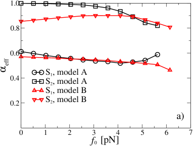
Figure 3: (Color online). (a) Transport power exponent $\alpha_{\rm eff}$ and (b) thermodynamic efficiency for the sets $S_{1,2}$ in the models A and B vs. loading force $f_{0}$. Notice that in the case $S_{2}$ the motor has an essentially larger efficiency within the model B than the model A, although the transport is more anomalous within the model B, especially for a small load. In part (b), full lines present fits with Eq. (21) with parameters shown in Table 2. Thermodynamic efficiency is calculated in accordance with Eq. (13) at the end point of simulations.

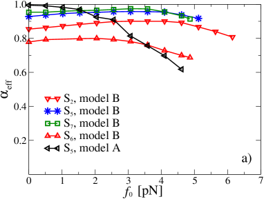
Figure 4: (Color online). (a) Transport power exponent $\alpha_{\rm eff}$ and (b) thermodynamic efficiency vs. loading force $f_{0}$ for several other sets shown in the plots and discussed in the text. In part (b), full lines present fits with Eq. (21) and parameters shown in Table 2. Thermodynamic efficiency is calculated in accordance with Eq. (13).

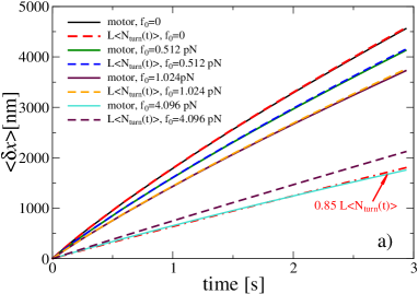
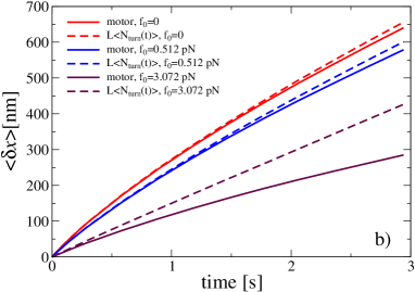
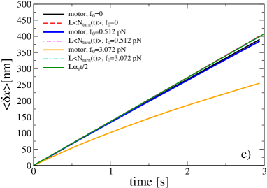
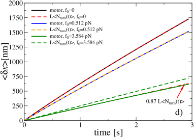
Figure 5: (color online). Mean motor displacement $\langle\delta x(t)\rangle$ and $L\langle N_{\rm turn}(t)\rangle$ vs. time for several values of $f_{0}$ shown in the plots for the sets: (a) $S_{2}$, model B; (b) $S_{6}$, model B; (c) $S_{5}$, model A; (d) $S_{5}$, model B. Good agreement between $\langle\delta x(t)\rangle$ and $L\langle N_{\rm turn}(t)\rangle$ reflects a perfect anomalous synchronization between stochastic turnovers of catalytic wheel and the motor stepping along microtubule. For small $f_{0}$ in the parts (a) and (d), increase of $f_{0}$ results in a synchronous slowing down of both the biochemical turnovers and the processive mechanical motion. It corresponds to a perfect anomalous ratchet regime. Even at the load corresponding to maximal thermodynamic efficiency in the cases (a) and (d), only about 15% and 13%, correspondingly, of ATP molecules consumed do not result into a perfect transport event – promotion on the length $L$ along microtubule. In part (c), $\langle N_{\rm turn}(t)\rangle$ practically does not depend on $f_{0}$ and is well described by $\alpha_{1}t/2$.

For a smaller cargo, sets $S_{2}$, the distinction between the models A and B becomes quite evident in Fig. 3. First, in the model A, $\alpha_{\rm eff}$ starts from $\alpha_{\rm eff}\approx 1$ at small $f_{0}$, and then it monotonously declines to about $0.8$ at the stalling force. In the model B, $\alpha_{\rm eff}\approx 0.854$ at $f_{0}=0$, see in the Table 3. It increases with $f_{0}$ to about $0.90$ at $f_{0}$ corresponding to the maximum of thermodynamic efficiency. After this, it declines to about $0.808$ at the stalling force, which is slightly larger than one within the model A.

III.0.1 Perfect subdiffusive ratchet

Within the model A, at small $f_{0}$ our motor realizes a perfect normal ratchet transport, where stochastic stepping along microtubule is perfectly synchronized with the normal turnovers of the catalytic wheel characterized by a turnover frequency equal to the half of the flashing frequency, Goychuk et al. (2014b), Goychuk (2015). A strikingly new result within the model B is that our ratchet realizes a perfect subtransport with anomalous turnovers of catalytic wheel which cannot be characterized anymore by a normal turnover frequency. Rather, one must introduce a new notion, the enzyme catalytic sub-velocity $\omega_{\gamma}$ by $\langle N_{\rm turn}(t)\rangle=\omega_{\gamma}t^{\gamma}/\Gamma(1+\gamma)$, see in the Supplementary Material. Notice that an attempt to define the standard turnover rate by $\lim_{t\to\infty}\langle N_{\rm turn}(t)\rangle/t$ would yield zero in this case. As Fig. 5, a and Table 3 reveal, for small $f_{0}$, $\alpha_{\rm eff}\approx\gamma<1$, and $\lambda\approx 0$. We are dealing with a perfect subdiffusive ratchet, where due to a mechano-chemical coupling, the consumption of ATP molecules by the motor scales sublinearly with time. Nevertheless, the transport is perfect in the sense that consumption of one ATP molecule leads to one step. Indeed, in Fig. 5, a, $\langle\delta x(t)\rangle$ almost coincides with $L\langle N_{\rm turn}(t)\rangle$ for $f_{0}=0$, $f_{0}=0.512$ pN, $f_{0}=1.024$ pN. Even for $f_{0}=4.096$ pN near to the $R_{\rm th}$ maximum, $\langle\delta x(t)\rangle\approx 0.85L\langle N_{\rm turn}(t)\rangle$, which means that only about 15% of biochemical turnovers do not lead to a successful step over $L$. $R_{\rm th}\approx 0.331$ at this maximum is much larger than in the model A, for small cargo, see in Fig. 3, a. Moreover, this perfect subdiffusive transport is very fast in absolute terms, cf. Fig. 5, a. Notice, that very differently from the model A, see in Fig. 5, c, the consumption of ATP molecules strongly depends on $f_{0}$ within the model B: it is smaller for larger $f_{0}$ (until about $f_{\rm max}$). This is a very important feature of the perfect subdiffusive ratchet mechanism. It is adaptive and economical.

The transport of the large cargo is far from being perfect in the case $S_{1}$, model B. However, maybe its quality can be drastically improved at smaller operational frequencies of the motor? Indeed, this is the case, as Fig. 4, and Fig. 5, b, reveal for the set $S_{6}$, model B. For a smaller $\alpha_{2}=17\;{\rm s^{-1}}$, $\alpha_{\rm eff}$ increases at $f_{0}=0$ from about $0.6$ (for $\alpha_{2}=170\;{\rm s^{-1}}$) to about $0.8$, see in the Table 4, and the maximum of $R_{\rm th}$ increases to about $0.2$, see in Fig. 4, b, i.e. it almost doubles, cf. Table 2. Even if the quality of anomalous synchronization is somewhat worser in this case than in the case $S_{2},B$ of smaller cargo, it is, nevertheless, quite impressive: a heavily loaded motor can walk over the distance of 650 nm at $f_{0}=0$ (which is normal operational regime of linear molecular motors in living cells) within the less than 3 sec, see in Fig. 5, b. Within the model A, transport of large cargo shares similar features for the parameter set $S_{5}$, with respect to thermodynamic efficiency, see in Fig. 4, b. However, the dependence of the transport exponent $\alpha_{\rm eff}$ on $f_{0}$ is entirely different. First, it features an almost normal transport at small $f_{0}$, cf. Fig.4, a, which is a nearly perfect, see in Fig. 5, c. Second, the turnover frequency of the enzyme practically does not depend on $f_{0}$, see in Fig. 5, c. It equals $\alpha_{1}/2$. Hence, with the increase of the static load $f_{0}$ strength, at the maximum of $R_{\rm th}$, $\alpha_{\rm eff}$ drops to about $0.81$, see in Table 5 and Fig. 4, while $\gamma$ remains one. This leads to a substantial decay of $R_{\rm th}\propto 1/t^{\lambda}$ in time, with $\lambda\approx 0.186$. Although, within the model B, set $S_{6}$, the decay of the maximum of $R_{\rm th}$ has about the same $\lambda\approx 0.196$, see in Table 4 at $f_{0}=3.072$ pN. This is so because in this case $\gamma$ arrives at the value of one for $f_{0}=3.072$ pN and larger. Hence, also in this respect, the models A and B are similar. However, once again, the stalling force is slightly larger in the model B.

III.0.2 The role of the rate $\alpha_{2}$

Next, it is interesting to clarify the influence of the rate $\alpha_{2}$, which is determined, in particular, by the ATP concentration (Astumian and Bier (1996), Jülicher et al. (1997), Parmeggiani et al. (1999)), on the transport properties within the model B. In fact, the sets $S_{2}$, $S_{5}$, and $S_{7}$ differ only by the value of $\alpha_{2}$. Fig. 4, b shows that the smaller is $\alpha_{2}$, the smaller is the maximum of thermodynamic efficiency, and the smaller is the stalling force. However, at the same time, smaller $\alpha_{2}$ corresponds to larger $\alpha_{\rm eff}$, see in Fig. 4, a, i.e. transport becomes closer to normal. Within the model B, the behavior of $\alpha_{\rm eff}$ versus $f_{0}$ displays one and the same universal feature. First, it slightly increases arriving at a maximum, and then it slightly drops. $\alpha_{\rm eff}$ is generally much less sensitive to $f_{0}$ within the model B, as compared to the model A. This is because within the model B the mechano-chemical coupling adjusts the tempo of biochemical cycling in response to $f_{0}$. It becomes slower. Fig.5, d and Table 6 demonstrate this effect for the set $S_{5}$, B. Once again, an almost perfect subdiffusive ratchet is realized for a sufficiently small cargo. At $f_{0}=3.584$ pN, which corresponds to the maximum of $R_{\rm th}$ of about 30%, only about 13% of the motor turnovers are futile, not resulting in a successful step along microtubule. A power-stroke like, mechano-chemically adaptive mechanism can lead to a perfect, energetically efficient subtransport.

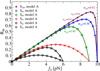
Figure 6: (Color online) Thermodynamic efficiency vs. loading force within model A for $U_{0}=25\;k_{B}T_{r}$ and $U_{0}=30\;k_{B}T_{r}$, as compared with the cases $S_{1,2}$, corresponding to $U_{0}=20\;k_{B}T_{r}$. Full lines present fits with Eq. (21) with parameters shown in Table 2. Notice a substantial increase of efficiency for larger $U_{0}$. It can exceed 80% in the case $S_{10}$. Here, numerical data present the results on the proper thermodynamic efficiency as described in the text. It is slightly larger than one in Eq. (13), see Fig. 6 in Goychuk (2015) and the corresponding discussion therein for detail.

III.0.3 Thermodynamic efficiency over 50%

Within the model A, the mechano-chemical coupling becomes also very essential, however, for a larger $U_{0}$. Then, thermodynamic efficiency can overcome 50%, even at the maximum of sub-power. Figs. 6, 7 demonstrate this striking effect. For the set $S_{10}$, thermodynamic efficiency exceeds 80% at its maximum, cf. Fig. 6. The maximum of $R_{\rm th}$ vs. $f_{0}$ in this case does not corresponds to thermodynamic efficiency at the maximum of sub-power $P_{\alpha}(f_{0})=v_{\alpha}(f_{0})f_{0}$ because of a strong mechano-chemical coupling. Nevertheless, the maximum of the latter one takes place at $f_{0}=7.168$ pN in Fig. 7, which corresponds approximately to impressive 70% in Fig. 6. Hence, we provided an instance of anomalous motor whose efficiency at maximal sub-power essentially exceeds 50%. This is a very important result. Very interesting is also dependence of the motor (sub)velocity on $f_{0}$ in this case. It drops to zero with increasing $f_{0}$ is a very non-linear fashion, which is very different from the low efficient quasi-linear regime, where it is nearly linear, Goychuk et al. (2014a, b). Similar nonlinearities were also observed experimentally for kinesin motors by Schnitzer et al. (2000) being, however, fitted in another way following a different model.

Figure 7: (Color online). Subpower $v_{\alpha}(f_{0})f_{0}$ (in the units of ${\rm pN\cdot nm/s^{\alpha_{\rm eff}}}$) and subvelocity (inset, in the units of ${\rm nm/s^{\alpha_{\rm eff}}}$) versus loading force, in the units of pN, for the set $S_{10}$, model A. $\alpha_{\rm eff}\approx 1$ for $f_{0}<5$ pN. Several other values are shown in the plot. At the maximum of subpower, at $f_{0}=7.168$, $\alpha_{\rm eff}\approx 0.9712$, and $\gamma\approx 0.9708$. Hence, the motor operates as a perfect subdiffusive ratchet whose thermodynamic efficiency at the subpower maximum is about 70%, in accordance with Fig. 6. The numerical data are fitted using Eq. (III) with $v_{\alpha}(0)=597.12\;{\rm nm/s^{\alpha_{\rm eff}}}$, $f_{\rm st}=9.91$ pN, $\epsilon=0.779$, and $q=-7.224$.

IV Discussion

The model B exhibits a much stronger mechano-chemical coupling than the model A. Within this model, mechano-chemical coupling is very essential already for $U_{0}=20\;k_{B}T_{r}$, which is a reasonable choice for kinesins II, given a typical stalling force of these motors. While the transport of a large cargo, like magnetosomes in Robert et al. (2010), looks very similar in both models, for a fast operating motor, the transport of smaller cargos is always profoundly different. The differences are also seen for slowly operating motors. Transport of the large cargo in this paper is characterized for $\alpha_{2}=170\;{\rm s^{-1}}$ by a transport exponent around $\alpha_{\rm eff}=0.6$ for $\alpha=0.4$, which can easily explain the observed superdiffusion exponents around $\beta=1.3\pm 0.1$ in the experiment, Robert et al. (2010). Energetically, such a transport is, however, inefficient. Nevertheless, while operating slower the motors can realize also energetically very efficient transport. Indeed, with a tenfold reduction of $\alpha_{2}$ from $170\;{\rm s}^{-1}$ to $17\;{\rm s}^{-1}$, such a near-to-perfect anomalous ratchet regime is realized for $f_{0}=0$ within the model B (set $S_{6}$) with $\alpha_{\rm eff}$ increased to about $0.8$. It should be noticed in this respect that normal modus operandi of linear motors like kinesin in living cells is one at near-to-zero thermodynamic efficiency. This should not confuse the readers because the useful work is done on overcoming the dissipative resistance of the environment while translocating cargo from one place to another one. Indeed, the chemical potential of neither motor, not cargo is typically increased. Hence, all the spent energy is eventually dissipated as heat. This is very different from the work of e.g. ionic pumps which must energize ions by transferring them against a corresponding electrochemical gradient. For pumps, namely the thermodynamic efficiency is of paramount importance and it must be optimized. Nevertheless, the ability to sustain substantial constant forces $f_{0}$ is important for a strong and good motor. It can be checked e.g. in the experiments with optical tweezers. Within the model B, the motor adapts its biochemical cycling to the increased $f_{0}$. It cycles slower and anomalously, while within the model A it cycles normally and at the same nearly constant tempo for $U_{0}=20\;k_{B}T_{r}$. This advantage of the model B is clearly seen for smaller cargos, where this study revealed a perfect and fast (in absolute terms) anomalous ratchet regime. The motor adapts it cyclic sub-velocity, and even at the maximum of thermodynamic efficiency, while working also against a strong $f_{0}$, the portion of the futile (in the transport sense) turnovers can be really small, just from 13% to 15%. This is definitely provides some benefits with respect to energetic costs of transport.

The mechano-chemical adaptation becomes also relevant within the model A, however, for larger $U_{0}$. We showed that for $U_{0}=0.75$ eV thermodynamic efficiency of our model motor can exceed 80% within an almost perfect anomalous ratchet regime while transferring smaller cargo against a large bias of $f_{0}=9$ pN with $\alpha_{\rm eff}\approx\gamma\approx 0.92$. Also efficiency at maximum sub-power can reach impressive 70% at $f_{0}\approx 7.2$ pN with $\alpha_{\rm eff}\approx\gamma\approx 0.97$. In such a thermodynamically highly efficient regime, the motor (sub)-velocity declines strongly nonlinearly with $f_{0}$. Indeed, similar nonlinearities were measured in some experiments with kinesins, Schnitzer et al. (2000). The very existence of such thermodynamically highly efficient regimes is especially inspiring when one thinks about perspectives of an optimal motor design, Cheng et al. (2015), Goychuk (2016). Clearly, a highly efficient operation is possible also in highly dissipative viscoelastic media like cytosol, as our study convincingly shows. This removes mental barriers and opens great perspectives for an optimal design of artificial molecular motors, Erbas-Cakmak et al. (2015), Cheng et al. (2015), especially in allowing to avoid some common fallacy traps, Goychuk (2016).

Notice, that within the both studied models of mechano-chemical coupling, we assumed either $\alpha_{1}$, or $\alpha_{2}$ be spatially-independent in a very large (half of the spatial period) region around the potential minima, so that neither $\nu_{1}(x)$, nor $\nu_{2}(x)$ turn zero somewhere on microtubule. Allosteric effects are nevertheless present because other rates are spatially dependent. They can be made stronger, when e.g. $\alpha_{1}$ in the model A is different from zero only in a small domain around the potential minimum. Strong allosteric effects are presumably very important for operating natural molecular motors and for designing the new ones, Cheng et al. (2015). Such effects can be used for a further optimization of the motor performance, which is very high already in the current, simplified and non-optimized version.

It should be also mentioned that two headed kinesins are highly processive motors, which means that they are attached to microtubule and walk on it before detaching for hundreds of steps and a sufficiently long time of several seconds, Hancock and Howard (1998), Alamilla and Santamaría-Holek (2012). In this respect, the maximal time in our simulations is about 3 sec. Our model is aimed to describe the transport during these processive periods. The influence of viscoelastic environment on their averaged duration, i.e. on the motor processivity, among other factors, Alamilla and Santamaría-Holek (2012), would also be a very interesting subject for future research, which requires, however, a further generalization of the model considered.

V Conclusions

To conclude, in this paper we extended our previous studies of anomalous transport of subdiffusing cargos by molecular motors in viscoelastic cytosol of living cells and showed the emergence of a perfect subdiffusive ratchet regime due to a mechano-chemical coupling. This anomalous transport regime is characterized by anomalously slow biochemical cycling of molecular motors accompanied by a sublinear consumption of ATP molecules in time, with their optimal use: consumption of one ATP molecule results in one step over the spatial period of microtubule, on average. Moreover, such a transport can be very fast in absolute terms, not bringing some disadvantages in this respect. Such anomalous transport regimes can be very important in the economics of living cells. Their assumed presence provides a true challenge for the experimentalists to reveal. The author hope and expect that the theoretical prediction of a slow consumption of ATP molecules by molecular motors, which cannot be characterized by a standard rate because both the number of enzyme turnovers and the amount of ATP consumed increase sublinearly in time, while transporting efficiently various cargos within interior of living cells, will eventually be confirmed experimentally.

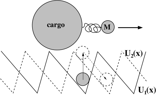
Figure 8: Grafical Abstract

Appendix A Supplementary Material

A.1 Numerical algorithm

In this section, a sketch of the numerical algorithm is presented. First, we rewrite Eqs. (7), (11), (12) of the main text as

$$\dot{x} = F(x,\zeta(t))+\nu_{m}G(x,y)+\sqrt{2D_{m}}\tilde{\xi}_{m}(t),$$ (16)

$$\dot{y} = -\nu_{c}G(x,y)-K(y,y_{i})+\sqrt{2D_{c}}\xi_{0}(t),$$

$$\dot{y_{i}} = \nu_{i}(y-y_{i})+\sqrt{2D_{i}}\xi_{i}(t),$$

where $D_{m}=k_{B}T/\eta_{m}$, $D_{c}=k_{B}T/\eta_{c}$, $D_{i}=k_{B}T/\eta_{i}$ are the corresponding diffusion coefficients, $F(x,\zeta(t))=[f(x,\zeta(t))-f_{0}]/\eta_{m}$, $G(x,y)=(y-x)/[1-(y-x)^{2}/r_{\rm max}^{2}]$, $K(y,y_{i})=\sum_{i=1}^{N}\nu_{i}(y-y_{i})$, $\nu_{m}=\kappa_{L}/\eta_{m}$, $\nu_{c}=\kappa_{L}/\eta_{c}$, and $\tilde{\xi}_{m}(t)$ is the scaled $\xi_{m}(t)$, $\langle\tilde{\xi}_{m}(t)\tilde{\xi}_{m}(t^{\prime})\rangle=\delta(t-t^{\prime})$. Notice that $F(x,\zeta(t))$ can take only two values: $F_{-}=[-(p+1)U_{0}/L-f_{0}]/\eta_{m}$ or $F_{+}=[(p+1)U_{0}/(pL)-f_{0}]/\eta_{m}$ depending on the motor position $x$ and conformational state $\zeta(t)=1$, or $\zeta(t)=2$. In the state ”1”: $F(x,1)=F_{-}$ for $x$ in the interval $[mL,mL+L/(p+1))$, and $F(x,1)=F_{+}$ for $x$ in the interval $[mL+L/(p+1),(m+1)L)$, where $m$ is an integer number. The values $F(x,2)=F(x+L/2,1)$. The values $F_{\pm}$ alternate in two ways: (i) deterministically depending on the motor position $x$, in the fixed motor state, and (ii) stochastically, when the motor state changes. The latter one is determined as follows. To integrate the system of stochastic differential equations (16) we use the stochastic Heun algorithm, Gard (1988). This implies that we iterate the time evolution in the discrete times steps $\Delta t$, $t_{k}=k\Delta t$. Then, for example, if the motor was in the state ”1” at $t_{k}$, the probability that it makes transition into the state ”2” during $\Delta t$ is $p_{1}=\nu_{1}(x_{k})\Delta t\ll 1$. Hence, one generates a random number $r$ from a uniform distribution on $[0,1]$. If $r\leq p_{1}$, the transition is done, and otherwise not. Typically, many iterations are required until a transition occurs. Similarly, for the current state ”2” with $p_{2}=\nu_{2}(x_{k})\Delta t\ll 1$. Furthermore, on each integration time step $\Delta t$ one generates anew $N+2$ independent zero-mean Gaussian variables $W_{i}$, $W_{m}$ with unit variance, $i=0,1,2...N$ (Mersenne Twister pseudo-random number generator was used for this). Each propagation step in the discretized time dynamics, $x_{k}=x(k\Delta t)$, $y_{k}=y(k\Delta t)$, $y_{i,k}=y_{i}(k\Delta t)$, from $t_{k}=k\Delta t$ to $t_{k+1}=t_{k}+\Delta t$ consists of two substeps. In the first substep,

$$x_{k}^{(1)} = x_{k}+\left[F(x_{k},\zeta)+\nu_{m}G(x_{k},y_{k})\right]\Delta t$$

$$+ \sqrt{2D_{m}\Delta t}W_{m},$$

$$y_{k}^{(1)} = y_{k}-[\nu_{c}G(x_{k},y_{k})+K(y_{k},y_{i,k})]\Delta t+\sqrt{2D_{c}\Delta t}W_{0},$$

$$y_{i,k}^{(1)} = y_{i,k}+\nu_{i}(y_{k}-y_{i,k})\Delta t+\sqrt{2D_{i}\Delta t}W_{i}\;.$$

In the second (final) step,

$$x_{k+1} = x_{k}+[F(x_{k}^{(1)},\zeta)+F(x_{k},\zeta)$$ (18)

$$+ \nu_{m}G(x_{k},y_{k})+\nu_{m}G(x_{k}^{(1)},y_{k}^{(1)})]\Delta t/2$$

$$+ \sqrt{2D_{m}\Delta t}W_{m},$$

$$y_{k+1} = y_{k}-[\nu_{c}G(x_{k},y_{k})+\nu_{c}G(x_{k}^{(1)},y_{k}^{(1)})$$

$$+ K(y_{k},y_{i,k})+K(y_{k}^{(1)},y_{i,k}^{(1)})]\Delta t/2+\sqrt{2D_{c}\Delta t}W_{0},$$

$$y_{i,k+1} = y_{i,k}+\nu_{i}(y_{k}+y_{k}^{(1)}-y_{i,k}-y_{i,k}^{(1)})\Delta t/2$$

$$+ \sqrt{2D_{i}\Delta t}W_{i}\;.$$

Notice that $W_{i}$ and $W_{m}$ must be the same numbers on the both substeps within each cycle of iterations, Gard (1988). The initial values $x_{0}=y_{0}=0$, at the minimum of potential $U_{1}(x)$ fixed initially, whereas $y_{0,i}$ are sampled from the corresponding Gaussian distributions, see the main text. They are different for each motor particle. The algorithm was implemented in CUDA and propagated in parallel (many different particles with different initially random preparations at the same time) on GPU processors.

A.2 Fitting dependencies

A biophysically inspired fitting form reads

$$v_{\alpha}(f)=v_{\alpha}(0)\left[1-\frac{f}{A+B\exp(-\delta f/(k_{B}T))}\right],$$ (19)

where $A,B$ are some constant with physical dimension of force and $\delta$ is some length. Such dependencies are common in biophysics, Phillips et al. (2013). Using the condition $v_{\alpha}(f_{\rm st})$, this expression can be readily expressed as Eq. (15) of the main text, with $q=A/f_{\rm st}$ and $\epsilon=\delta f_{\rm st}/(k_{B}T)$.

Another reasonable form is, Goychuk (2016),

$$v_{\alpha}(f_{0})=v_{\alpha}(0)[1-(f_{0}/f_{\rm st})^{a}]$$ (20)

with some fitting power exponent $a$. It has one parameter less. However, a possible interpretation of $a$ is not clear. Then, Eq. (14) is replaced by

$$R_{\rm th}(f_{0})=k\frac{f_{0}}{f_{\rm st}}\left[1-\left(\frac{f_{0}}{f_{\rm st}}\right)^{a}\right].$$ (21)

A certain advantage is that the maximal value of $R_{\rm th}^{(\rm max)}=ka/(1+a)^{1+1/a}$ at $f_{\rm max}=f_{\rm st}/(1+a)^{1/a}$ can be readily found in analytical form. The corresponding fits with the parameters in the Table 2 are shown in Figs. 9, 10, 11, which correspond to Figs. 3b, 4b, 6, of the main text, respectively. One can see that this alternative fit is really not bad. However, in Fig. 6 of the main text the fitting of two upper curves with Eq. (14) is much better, on the cost of having one parameter more. Actually with $q=0$ in Eq. (14), having the same number of fitting parameters, the both fits are equally good (not shown). However, interpretation of the power exponent $a$, which can take values as large as $52.26$, see in Table 7, is rather dim. Notice that the inset of Fig. 12, which corresponds to Fig. 7 of the main text, contains yet another fit related to (20).

Table 7: Parameters of the fit $R_{\rm th}(f_{0})=k(f_{0}/f_{\rm st})\left[1-(f_{0}/f_{\rm st})^{a}\right]$, and the corresponding values of $R_{\rm th}^{(\rm max)}$, and $f_{\rm max}$

Set, Model	$k$	$f_{\rm st}$, pN	$a$	$R_{\rm th}^{(\rm max)}$	$f_{\rm max}$,pN
$S_{1},A$	0.385	6.00	1.112	0.103	3.06
$S_{2}$, A	0.418	5.91	4.925	0.242	4.12
$S_{5}$, A	0.454	4.79	2.405	0.192	2.88
$S_{7}$, A	0.758	9.00	1.94	0.287	5.16
$S_{8}$, A	0.909	10.00	20.08	0.744	8.59
$S_{9}$, A	0.847	9.00	8.93	0.589	6.96
$S_{10}$, A	0.952	10.00	52.26	0.866	9.27
$S_{1}$, B	0.4193	6.282	0.982	0.104	3.13
$S_{2}$, B	0.615	6.24	3.865	0.324	4.14
$S_{5}$, B	0.522	5.36	4.746	0.298	3.71
$S_{6}$, B	0.493	5.01	2.148	0.197	2.94
$S_{7}$, B	0.489	5.01	4.619	0.277	3.45

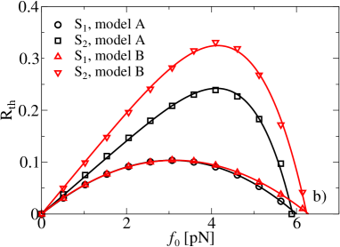
Figure 9: Thermodynamic efficiency for the sets $S_{1,2}$ in the models A and B vs. loading force $f_{0}$. Full lines present fits with Eq. (21) with parameters shown in Table 2.

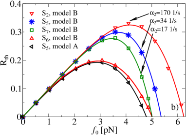
Figure 10: Thermodynamic efficiency vs. loading force $f_{0}$ for several other sets shown in the plots and discussed in the main text. Full lines present fits with Eq. (21) and parameters shown in Table 2.

Figure 11: Thermodynamic efficiency vs. loading force within model A for $U_{0}=25\;k_{B}T_{r}$ and $U_{0}=30\;k_{B}T_{r}$, as compared with the cases $S_{1,2}$, corresponding to $U_{0}=20\;k_{B}T_{r}$. Full lines present fits with Eq. (21) with parameters shown in Table 2.

Figure 12: (Color online). Subpower $v_{\alpha}(f_{0})f_{0}$ (in the units of ${\rm pN\cdot nm/s^{\alpha_{\rm eff}}}$) and subvelocity (inset, in the units of ${\rm nm/s^{\alpha_{\rm eff}}}$) versus loading force, in the units of pN, for the set $S_{10}$, model A. The numerical data in inset are fitted by the dependence $v_{\alpha}(f_{0})=v_{1}(0)\left[1-(f_{0}/f_{1})^{2}-(f_{0}/f_{2})^{a_{2}}\right]$, with $v_{1}(0)=597.12$ nm/s, $f_{1}=15.60$ pN, $f_{2}=10.52$ pN, and $a_{2}=9.258$. Fit with Eq. (20) (not shown) is essentially worser.

A.3 Simplest model for anomalous enzyme dynamics

One of the major results of this paper is that biochemical cycling of a motor enzyme can become anomalously slow and synchronize with its mechanical motion along microtubule, $\gamma\approx\alpha_{\rm eff}<1$, due to influence of viscoelastic environment via a mechano-chemical coupling. This finding can be rationalized within the following (over)simplified model. Cycling of a motor enzyme in its intrinsic conformational space can be parametrized by an angle variable $\phi$. It occurs on a periodic free-energy landscape biased due to energy released in ATP hydrolysis $G(\phi)=G_{0}(\phi)-\Delta G_{\rm ATP}\phi/(2\pi)$ (Nelson (2003), Schnitzer et al. (2000), Alamilla and Santamaría-Holek (2012), Goychuk (2016)), $G_{0}(\phi+2\pi)=G_{0}(\phi)$. In other words, $\Delta G_{\rm ATP}$ produces a driving torque $M_{\rm st}=\Delta G_{\rm ATP}/2\pi$. The mechanical load $f_{0}$ will produce a counter-acting torque $M_{0}=f_{0}L/2\pi$. Here, we assume a perfect synchronization between the mechanical motion and the enzymatic turnover, Nelson (2003). Furthermore, let us assume that the conformational motion is subjected to normal and anomalous frictions and the corresponding noise terms, which are related by the fluctuation-dissipation relation (FDR), $\langle\zeta_{0}(t)\zeta_{0}(t^{\prime})\rangle=2k_{B}Tr_{0}\delta(t-t^{\prime})$, $\langle\zeta_{\gamma}(t)\zeta_{\gamma}(t^{\prime})\rangle=k_{B}Tr_{\gamma}/|t-t^{\prime}|^{\gamma}$. Then, it can be described by a generalized Langevin equation (GLE)

$$r_{0}\dot{\phi} = -\frac{\partial G_{0}(\phi)}{\partial\phi}+M_{\rm st}-M_{0}+\zeta_{0}(t)$$

$$- r_{\gamma}\frac{d^{\gamma}\phi}{dt^{\gamma}}+\zeta_{\gamma}(t)\;,$$

where $\frac{d^{\gamma}\phi}{dt^{\gamma}}$ is the Caputo fractional derivative, (Gorenflo and Mainardi (1997), Mathai and Haubold (2017)). The just formulated model presents a fractional conformational dynamics generalization of the simplest model of molecular motors, see e.g. in Goychuk (2016). The mechanical stalling force is $f_{\rm st}=2\pi M_{\rm st}/L=\Delta G_{\rm ATP}/L$, within this model. With $\Delta G_{\rm ATP}=20\;k_{B}T_{r}=82\;{\rm pN\cdot nm}$, and $L=8$ nm this yields $f_{\rm st}=10.25$ pN, which indeed is slightly larger than the maximal stalling force of 10 pN in the main text for $U_{0}=30\;k_{B}T_{r}$. Furthermore, as shown in Goychuk (2009, 2012b), in the case of viscoelastic subdiffusion a static spatially periodic potential does not influence asymptotically diffusion and transport. Hence, with $t\to\infty$, the number of enzymatic turnovers grows sublinearly as

$$\langle N_{\rm turn}(t)\rangle\sim\omega_{\gamma}t^{\gamma}/\Gamma(1+\gamma),$$ (23)

where $\omega_{\gamma}=(M_{\rm st}-M_{0})/r_{\gamma}$ can be termed the catalytic sub-velocity of enzyme. Because the useful work done against the load is $W_{\rm use}(t)\sim f_{0}\langle\delta x(t)\rangle=f_{0}L\langle\phi(t)\rangle/2\pi\propto t^{\gamma}$ within this model, the thermodynamic efficiency $R_{\rm th}$ is time-independent, and $v_{\alpha=\gamma}(0)=\omega_{\gamma}L$ in Eq. (20). In the $t\to\infty$ limit, $R_{\rm th}$ is given by Eq. (21) with $k=1$ and $a=1$. It arrives at the maximum of 50% at $f_{\rm max}=f_{\rm st}/2$.

Of course, the just outlined simplest model of anomalous enzyme turnovers does not correspond precisely to the model in the main text, in some very important detail. First, it restricts the efficiency at maximal sub-power by 50% – the Jacobi bound, and corresponds to a symmetric parabolic $R_{\rm th}$ in Eq. (21) with $k=1$, $a=1$. Second, the motor dynamics in the main text was assumed to be normal, memoryless in the absence of a coupled cargo. So, where the memory terms in Eq. (A.3), the second line, can come from, in principle? The point is that we have to consider some coupling energy $G(\phi,x)$ instead of $G(\phi)$ and to exclude the dynamics of the $x(t)$ variable. Such a procedure generally leads to a memory friction and the related noise in the $\phi$ dynamics considered alone. This is what is assumed in our ultimately simplified model, which does not contain, however, a theory for $\gamma\approx\alpha_{\rm eff}$. In this respect, it must be noted that nonlinear effects in the case of a spatially periodic but fluctuating $G_{0}(\phi,t)$ are generally very important, Goychuk (2012b). This is the reason why such an oversimplified model cannot describe, e.g., thermodynamic efficiencies over 50% at the maximum of sub-power, as found and described in the main text.

References

- (1)
- Ajdari and Prost (1992) Ajdari, A. and Prost, J.: 1992, Mouvement induit par un potentiel pèriodique de basse symètrie: dièlectrophorese pulsèe, Comp. Rend Acad. Sci., Paris II 315, 1635–1639.
- Alamilla and Santamaría-Holek (2012) Alamilla, N. J. L. and Santamaría-Holek, I.: 2012, Reconstructing the free-energy landscape associated to molecular motor processivity, Biophys. Chem. 167, 16–25.
- Amblard et al. (1996) Amblard, F., Maggs, A. C., Yurke, B., Pargellis, A. N. and Leibler, S.: 1996, Subdiffusion and anomalous local viscoelasticity in actin networks, Phys. Rev. Lett. 77, 4470–4473.
- Astumian and Bier (1994) Astumian, R. D. and Bier, M.: 1994, Fluctuation driven ratchets: Molecular motors, Phys. Rev. Lett. 72, 1766–1769.
- Astumian and Bier (1996) Astumian, R. D. and Bier, M.: 1996, Mechanochemical coupling of the motion of molecular motors to atp hydrolysis, Biophys. J. 70, 637.
- Baker et al. (2001) Baker, N. A., Sept, D., Joseph, S., Holst, M. J. and McCammon, J. A.: 2001, Electrostatics of nanosystems: Application to microtubules and the ribosome, Proc. Nat. Acad. Sci. USA 98, 10037.
- Banks and Fradin (2005) Banks, D. S. and Fradin, C.: 2005, Anomalous diffusion of proteins due to molecular crowding, Biophys. J. 89, 2960–2971.
- Bartussek et al. (1994) Bartussek, R., Hänggi, P. and Kissner, J. G.: 1994, Periodically rocked thermal ratchets, EPL (Europhysics Letters) 28(7), 459.
- Bochud and Challet (2007) Bochud, T. and Challet, D.: 2007, Optimal approximations of power laws with exponentials: application to volatility models with long memory, Quantitative Finance 7(6), 585–589.
- Bruno et al. (2009) Bruno, L., Levi, V., Brunstein, M. and Desposito, M. A.: 2009, Transition to superdiffusive behavior in intracellular actin-based transport mediated by molecular motors, Phys. Rev. E 80, 011912.
- Bruno et al. (2011) Bruno, L., Salierno, M., Wetzler, D. E., Desposito, M. A. and Levi, V.: 2011, Mechanical properties of organelles driven by microtubuli-dependent molecular motors in living cells, PLoS ONE 6, e18332.
- Caspi et al. (2002) Caspi, A., Granek, R. and Elbaum, M.: 2002, Diffusion and directed motion in cellular transport, Phys. Rev. E 66, 011916.
- Cheng et al. (2015) Cheng, C., McGonigal, P. R., Stoddart, J. F. and Astumian, R. D.: 2015, Design and synthesis of nonequilibrium systems, ACS Nano 9, 8672–8688.
- Doering et al. (1994) Doering, C. R., Horsthemke, W. and Riordan, J.: 1994, Nonequilibrium fluctuation-induced transport, Phys. Rev. Lett. 72, 2984–2987.
- Erbas-Cakmak et al. (2015) Erbas-Cakmak, S., Leigh, D. A., McTernan, C. T. and Nussbaumer, A. L.: 2015, Artificial molecular machines, Chem. Rev. 115, 10081–10206.
- Gard (1988) Gard, T. C.: 1988, Introduction to Stochastic Differential Equations, Dekker, New York.
- Gittes et al. (1997) Gittes, F., Schnurr, B., Olmsted, P. D., MacKintosh, F. C. and Schmidt, C. F.: 1997, Microscopic viscoelasticity: Shear moduli of soft materials determined from thermal fluctuations, Phys. Rev. Lett. 79, 3286–3289.
- Golding and Cox (2006) Golding, I. and Cox, E. C.: 2006, Physical nature of bacterial cytoplasm, Phys. Rev. Lett. 96, 098102.
- Gorenflo and Mainardi (1997) Gorenflo, R. and Mainardi, F.: 1997, in A. Carpinteri and F. Mainardi (eds), Fractal and Fractal Calculus in Continuum Mechanics, Springer, Wien, pp. 223–276.
- Goychuk (2009) Goychuk, I.: 2009, Viscoelastic subdiffusion: from anomalous to normal, Phys. Rev. E 80, 046125.
- Goychuk (2010) Goychuk, I.: 2010, Subdiffusive brownian ratchets rocked by a periodic force, Chem. Phys. 375, 450–457.
- Goychuk (2012a) Goychuk, I.: 2012a, Fractional time random walk subdiffusion and anomalous transport with finite mean residence times: faster, not slower, Phys. Rev. E 86, 021113.
- Goychuk (2012b) Goychuk, I.: 2012b, Viscoelastic subdiffusion: Generalized langevin equation approach, Adv. Chem. Phys. 50, 187–253.
- Goychuk (2015) Goychuk, I.: 2015, Anomalous transport of subdiffusing cargos by single kinesin motors: the role of mechanochemical coupling and anharmonicity of tether, Phys. Biol. 12, 016013.
- Goychuk (2016) Goychuk, I.: 2016, Molecular machines operating on the nanoscale: from classical to quantum, Beilstein J. Nanotechnol. 7, 328–350.
- Goychuk (2018) Goychuk, I.: 2018, Viscoelastic subdiffusion in a random gaussian environment, Phys. Chem. Chem. Phys. 20, 24140–24155.
- Goychuk and Hänggi (2002) Goychuk, I. and Hänggi, P.: 2002, Ion channel gating: A first-passage time analysis of the kramers type, Proc. Natl. Acad. Sci. (USA) 99(6), 3552–3556.
- Goychuk and Kharchenko (2012) Goychuk, I. and Kharchenko, V.: 2012, Fractional brownian motors and stochastic resonance, Phys. Rev. E 85, 051131.
- Goychuk and Kharchenko (2013) Goychuk, I. and Kharchenko, V. O.: 2013, Rocking subdiffusive ratchets: origin, optimization and efficiency, Math. Model. Nat. Phenom. 8, 144–158.
- Goychuk et al. (2014a) Goychuk, I., Kharchenko, V. O. and Metzler, R.: 2014a, How molecular motors work in the crowded environment of living cells: Coexistence and efficiency of normal and anomalous transport, PLoS ONE 9, e91700.
- Goychuk et al. (2014b) Goychuk, I., Kharchenko, V. O. and Metzler, R.: 2014b, Molecular motors pulling cargos in the viscoelastic cytosol: how power strokes beat subdiffusion, Phys. Chem. Chem. Phys. 16, 16524.
- Guigas et al. (2007) Guigas, G., Kalla, C. and Weiss, M.: 2007, Probing the nanoscale viscoelasticity of intracellular fluids in living cells, Biophys. J. 93, 316.
- Hancock and Howard (1998) Hancock, W. O. and Howard, J.: 1998, Processivity of the motor protein kinesin requires two heads, J. Cell Biol. 140, 1395–1405.
- Harrison et al. (2013) Harrison, A. W., Kenwright, D. A., Waigh, T. A., Woodman, P. G. and Allan, V. J.: 2013, Modes of correlated angular motion in live cells across three distinct time scales, Phys. Biol. 10, 036002.
- Herrchen and Öttinger (1997) Herrchen, M. and Öttinger, H. C.: 1997, A detailed comparison of various fene dumbbell models, J. Non-Newtonian Fluid Mech. 68, 17.
- Hill (1989) Hill, T. L.: 1989, Free Energy Transduction and Biochemical Cycle Kinetics, Springer, New York.
- Hirokawa and Takemura (2005) Hirokawa, N. and Takemura, T.: 2005, Molecular motors and mechanisms of directional transport in neurons, Nature Reviews 6, 201–214.
- Hughes (1995) Hughes, B. D.: 1995, Random Walks and Random Environments, Clarendon Press, Oxford.
- Jeon et al. (2012) Jeon, J.-H., Monne, H. M.-S., Javanainen, M. and Metzler, R.: 2012, Anomalous diffusion of phospholipids and cholesterols in a lipid bilayer and its origins, Phys. Rev. Lett. 109, 188103.
- Jeon et al. (2011) Jeon, J. H., Tejedor, V., Burov, S., Barkai, E., Selhuber-Unkel, C., Berg-Sørensen, K., Oddershede, L. and Metzler, R.: 2011, In vivo anomalous diffusion and weak ergodicity breaking of lipid granules, Phys. Rev. Lett. 106, 048103.
- Jülicher et al. (1997) Jülicher, F., Ajdari, A. and Prost, J.: 1997, Modeling molecular motors, Rev. Mod. Phys. 69, 1269.
- Kharchenko and Goychuk (2012) Kharchenko, V. O. and Goychuk, I.: 2012, Flashing subdiffusive ratchets in viscoelastic media, New J. Phys. 14, 043042.
- Kharchenko and Goychuk (2013) Kharchenko, V. O. and Goychuk, I.: 2013, Subdiffusive rocking ratchets in viscoelastic media: Transport optimization and thermodynamic efficiency in overdamped regime, Phys. Rev. E 87, 052119.
- Kneller et al. (2011) Kneller, G. R., Baczynski, K. and Pasenkiewicz-Gierula, M.: 2011, Communication: Consistent picture of lateral subdiffusion in lipid bilayers: Molecular dynamics simulation and exact results, J. Chem. Phys. 135, 141105.
- Kojima et al. (1996) Kojima, H., Muto, E., Higuchi, H. and Yanagida, T.: 1996, Mechanics of single kinesin molecules measured by optical trapping nanometry, Biophys. J 73, 2012.
- Kolmogorov (1940) Kolmogorov, A. N.: 1940, Wiener spirals and some other interesting curves in a hilbert space, Dokl. Akad. Nauk SSSR 26, 115–118 (in Russian).
- Kolmogorov (1991) Kolmogorov, A. N.: 1991, Wiener spirals and some other interesting curves in a hilbert space, in V. M. Tikhomirov (ed.), Selected Works of A. N. Kolmogorov, vol. I, Mechanics and Mathematics, Kluwer, Dordrecht, pp. 303–307.
- Kubo (1966) Kubo, R.: 1966, Fluctuation-dissipation theorem, Rep. Prog. Theor. Phys. 29, 255.
- Larson (1999) Larson, R. G.: 1999, The Structure and Rheology of Complex Fluids, Oxford University Press, New York.
- Luby-Phelps (2013) Luby-Phelps, K.: 2013, The physical chemistry of cytoplasm and its influence on cell function: an update, Mol. Biol. Cell 24, 2593.
- Magnasco (1993) Magnasco, M. O.: 1993, Forced thermal ratchets, Phys. Rev. Lett. 71, 1477–1481.
- Makhnovskii et al. (2004) Makhnovskii, Y. A., Rozenbaum, V. M., Yang, D.-Y., Lin, S. H. and Tsong, T. Y.: 2004, Flashing ratchet model with high efficiency, Phys. Rev. E 69, 021102.
- Mandelbrot and van Ness (1968) Mandelbrot, B. and van Ness, J.: 1968, Fractional brownian motion, fractional gaussian noise and applications, SIAM Rev. 10, 422.
- Mason and Weitz (1995) Mason, T. G. and Weitz, D. A.: 1995, Optical measurements of frequency-dependent linear viscoelastic moduli of complex fluids, Phys. Rev. Lett. 74, 1250–1253.
- Mathai and Haubold (2017) Mathai, A. M. and Haubold, H. J.: 2017, An Introduction to Fractional Calculus, Nova Science Publishers, New York.
- Nelson (2003) Nelson, P.: 2003, Biological Physics: Energy, Information, Life, W. H. Freeman, New York.
- Palmer et al. (1984) Palmer, R. G., Stein, D. L., Abrahams, E. and Anderson, P. W.: 1984, Models of hierarchically constrained dynamics for glassy relaxation, Phys. Rev. Lett. 53, 958–961.
- Pan et al. (2009) Pan, W., Filobelo, L., Pham, N. D. Q., Galkin, O., Uzunova, V. V. and Vekilov, P. G.: 2009, Viscoelasticity in homogeneous protein solutions, Phys. Rev. Lett. 102, 058101.
- Parmeggiani et al. (1999) Parmeggiani, A., Jülicher, F., Ajdari, A. and Prost, J.: 1999, Energy transduction of isothermal ratchets: Generic aspects and specific examples close to and far from equilibrium, Rev. Rev. E 60, 2127.
- Phillips et al. (2013) Phillips, R., Kondev, J., Theriot, J. and Garcia, H. G.: 2013, Physical Biology of the Cell, 2nd edn, Garland Science, London.
- Pollard et al. (2008) Pollard, T. D., Earnshaw, W. C. and Lippincott-Schwarz, J.: 2008, Cell Biology, 2nd edn, Saunders Elsevier, Philadelphia.
- Prost et al. (1994) Prost, J., Chauwin, J.-F. m. c., Peliti, L. and Ajdari, A.: 1994, Asymmetric pumping of particles, Phys. Rev. Lett. 72, 2652–2655.
- Qian (2005) Qian, H.: 2005, Cycle kinetics, steady state thermodynamics and motors – a paradigm for living matter physics, J. Phys. Cond. Matt. 17, S3783–S3794.
- Reimann (2002) Reimann, P.: 2002, Brownian motors: noisy transport far from equilibrium, Phys. Rep. 361, 57–265.
- Robert et al. (2010) Robert, D., Nguyen, T.-H., Gallet, F. and Wilhelm, C.: 2010, Diffusion and directed motion in cellular transport, PLoS ONE 4, e10046.
- Rousselet et al. (1994) Rousselet, J., Salome, L., Ajdari, A. and Prost, J.: 1994, Directional motion of brownian particles induced by a periodic asymmetric potential, Nature (London) 370, 446.
- Rozenbaum et al. (2004) Rozenbaum, V. M., Yang, D.-Y., Lin, S. H. and Tsong, T. Y.: 2004, Catalytic wheel as a brownian motor, J. Phys. Chem. B 108, 15880–15889.
- Santamaría-Holek et al. (2007) Santamaría-Holek, I., Rubí, J. M. and Gadomski, A.: 2007, Thermokinetic approach of single particles and clusters involving anomalous diffusion under viscoelastic response, J. Phys. Chem. B 111, 2293–2298.
- Saxton and Jacobson (1997) Saxton, M. J. and Jacobson, K.: 1997, Single-particle tracking: applications to membrane dynamics, Annu. Rev. Biophys. Biomol. Struct. 26, 373.
- Schnitzer et al. (2000) Schnitzer, M. J., Visscher, K. and Block, S. M.: 2000, Force production by single kinesin motors, Nature Cell Biology 2, 718–723.
- Seisenberger et al. (2001) Seisenberger, G., Ried, M. U., Endress, T., Büning, H., Hallek, M. and Bräuchle, C.: 2001, Real-time single-molecule imaging of the infection pathway of an adeno-associated virus, Science 294, 1929–1932.
- Svoboda et al. (1993) Svoboda, K., Schmidt, C. F., Schnapp, B. J. and Block, S. M.: 1993, Direct observation of kinesin stepping by optical trapping interferometry, Nature (London) 365, 721–727.
- Tabei et al. (2013) Tabei, S. M. A., Burov, S., Kima, H. Y., Kuznetsov, A., Huynha, T., Jureller, J., Philipson, L. H., Dinner, A. R. and Scherer, N. F.: 2013, Intracellular transport of insulin granules is a subordinated random walk, Proc. Natl. Acad. Sci. (USA) 110, 4911–4916.
- Tolic-Norrelykke et al. (2004) Tolic-Norrelykke, I. M., Munteanu, E.-L., Thon, G., Oddershede, L. and Berg-Sorensen, K.: 2004, Anomalous diffusion in living yeast cells, Phys. Rev. Lett. 93, 078102.
- Turner (2005) Turner, P. J.: 2005, XMGRACE, Version 5.1.19, Center for Coastal and Land-Margin Research, Oregon Graduate Institute of Science and Technology, Beaverton, OR.
- Waigh (2005) Waigh, T. A.: 2005, Microrheology of complex fluids, Rep. Progr. Phys. 68, 685.
- Weigel et al. (2011) Weigel, A. V., Simon, B., Tamkun, M. M. and Krapf, D.: 2011, Ergodic and nonergodic processes coexist in the plasma membrane as observed by single-molecule tracking, Proc. Natl. Acad. Sci. (USA) 108, 6438–6443.
- Weiss (2013) Weiss, M.: 2013, Single-particle tracking data reveal anticorrelated fractional brownian motion in crowded fluids, Phys. Rev. E 88, 010101.
- Weiss et al. (2004) Weiss, M., Elsner, M., Kartberg, F. and Nilsson, T.: 2004, Anomalous subdiffusion is a measure for cytoplasmic crowding in living cells, Biophys. J. 87, 3518–3524.
- Weiss (1999) Weiss, U.: 1999, Quantum Dissipative Systems, 2nd edn, World Scientific, Singapore.
- Wyman (1975) Wyman, J.: 1975, The turning wheel: a study in steady states, Proc. Nat. Acad. Sci. USA 72, 3983.
- Zwanzig (2001) Zwanzig, R.: 2001, Nonequilibrium Statistical Mechanic, Oxford University Press, Oxford.